When Shock Waves Collide

Abstract

Supersonic outflows from objects as varied as stellar jets, massive stars and novae often exhibit multiple shock waves that overlap one another. When the intersection angle between two shock waves exceeds a critical value, the system reconfigures its geometry to create a normal shock known as a Mach stem where the shocks meet. Mach stems are important for interpreting emission-line images of shocked gas because a normal shock produces higher postshock temperatures and therefore a higher-excitation spectrum than an oblique one does. In this paper we summarize the results of a series of numerical simulations and laboratory experiments designed to quantify how Mach stems behave in supersonic plasmas that are the norm in astrophysical flows. The experiments test analytical predictions for critical angles where Mach stems should form, and quantify how Mach stems grow and decay as intersection angles between the incident shock and a surface change. While small Mach stems are destroyed by surface irregularities and subcritical angles, larger ones persist in these situations, and can regrow if the intersection angle changes to become more favorable. The experimental and numerical results show that although Mach stems occur only over a limited range of intersection angles and size scales, within these ranges they are relatively robust, and hence are a viable explanation for variable bright knots observed in HST images at the intersections of some bow shocks in stellar jets.

1 Introduction

Supersonic flows in astrophysics often contain multiple shock fronts that form as a result of unsteady outflows. Examples include supernovae remnants (Chevalier & Theys, 1975; Anderson et al., 1994), shells of novae (Shara et al., 1997), and Herbig-Haro (HH) bow shocks (Hartigan et al., 2001). High-resolution images of these objects sometimes show bright knots where the shock fronts intersect, and the motion of these knots differs from the overall motion of their parent shocks (Hartigan et al., 2011). It is important to understand the different types of geometries that are possible at intersection points of shocks because the postshock temperature, and therefore the line excitation, depends upon the orientation of the shock relative to motion of the incident gas. In addition, if a bright knot in a jet merely traces the intersection point, then its observed proper motion will follow the location of that point and will not represent the bulk motion of the shock wave. Even bow shocks that appear smooth in ground-based images can be affected by this phenomenon. For example, the stellar jet bow shocks HH 1 and HH 47 both exhibit variable filamentary structure in the highest-resolution HST images that most likely arises from irregularities in the shock surfaces (Hartigan et al., 2011). Hence, to interpret both the emission line structure and the observed kinematics of astrophysical shock waves accurately we must understand the physics of shock intersections.

The theory of intersecting shock fronts is complex and has been studied for over a century. Modern reviews such as Ben-Dor (2007) summarize a variety of shock geometries that arise when shock waves collide. Early theoretical work by von Neumann (1943) laid the foundation for the field by identifying two general classes of solutions to the hydrodynamic equations at shock intersections that he labeled as regular reflection (RR) and Mach reflection (MR; Fig. 1). Regular reflection occurs in the case of intersecting bow shocks when the apices of two bows are far apart and the shock waves intersect at an acute angle in the wings of the bows. As shown in Fig. 1, by symmetry, the gas that lies along the axis between the two bows will have no net lateral deflection. Hence, a pair of reflected shocks must form behind the intersection point between the bows that redirects the flow along the axis of symmetry.

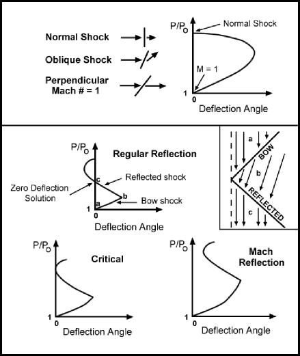
Figure 2: Shock polars. Top: As the incident angle of the preshock gas to a planar shock increases, the deflection angle first increases and then decreases. The ratio of the postshock to preshock pressures is denoted as P/P_∘. Bottom: Two oblique shock waves that deflect gas in opposite directions may either generate two, one, or zero solutions that cross the y-axis in a polar diagram. These cases correspond to regular reflection, critical, and Mach reflection, respectively. The inset depicts regular reflection.

As shown in the top panel of Fig. 2, the amount that a planar shock deflects the incident gas depends upon the angle of the shock to the flow. Normal shocks produce zero deflection, and shocks that are inclined at the Mach angle, defined so the perpendicular component of the velocity relative to the front has a Mach number of 1, also do not deflect the incident gas. At intermediate angles the shock deflects the gas away from the shock normal, and the deflection goes through a maximum. Plots of the deflection angle as a function of the effective Mach number squared (or the ratio of the postshock pressure to the preshock pressure) are known as shock polars (Kawamura & Saito, 1956). As depicted in Fig. 2, one can determine the net amount of deflection from two planar shocks (in this case the bow shock and its reflection shock) by attaching two polar curves together at the point where the two shocks intersect. As one moves up along the reflected shock curve in Fig. 2 it is the equivalent of changing the orientation angle of the reflected shock.

When the two bow shocks are widely-separated, their intersection point lies far into the wings of the bows. Material entering the bow shocks near this point encounters a weak shock with a small deflection angle. The bottom panel of Fig 2 shows that when the bow shock is weak (P/P_∘ $\sim$ 1), the reflected shock polar crosses the x-axis at two locations, implying there are two solutions with zero net deflection (in practice, systems choose the smaller value that corresponds to the weaker shock; Ben-Dor, 2007). However, if the bow shocks are close together, the intersection angle between the shocks becomes more oblique, and a critical point is reached where there is no solution for zero deflection. At more oblique angles than the critical point, the system reconfigures to Mach reflection (Fig. 1), consisting of the bow shock, reflected shock, and a Mach stem that intersect at a triple point. Eventually, as the apices of the bow shocks approach one-another the lateral motion behind the bow shocks becomes subsonic and the triple point goes away, leaving the system with single bow shock. Theoretically, Courant & Friedrichs (1948) give an equation for the critical angle in the limit of high Mach numbers as

$$\alpha_{C}=sin^{-1}\left(\frac{1}{\gamma}\right)$$ (1)

where $\gamma$ is the adiabatic index of the gas. A similar, but more detailed analytical expression was derived by De Rosa et al. (1992).

When the interaction angle rises above the critical angle, the RR should transition to MR, and the system should return to RR if the critical angle decreases. Theoretically, both MR and RR may occupy the same parameter space (Li & Ben Dor, 1996), and there is experimental evidence that the mode present in a given situation depends upon the previous history of the gas, a phenomenon referred to as hysteresis. As described by Ben-Dor et al. (2002) and Chpoun et al. (1995), the critical angle for RR $\rightarrow$ MR differs slightly from the critical angle for MR $\rightarrow$ RR. In addition, under some circumstances the region near the triple point can become more complex, and even split into dual triple points known as double Mach-reflection (hereafter DMR; White, 1951; Hu & Glass, 1986). These DMR structures involve rather small changes to the overall shock geometry compared with the normal Mach stem case and currently have no obvious astrophysical analogs.

Experimentally, most of the effort to date regarding the MR $\leftrightarrow$ RR transition has been directed to studying relatively low Mach number flows. Exploring the physics of Mach stems at high Mach numbers has recently become possible on experimental platforms that use intense lasers to drive strong shocks. One such platform, developed by Foster et al. (2010) on the University of Rochester’s Omega laser, drove pairs of strong shocks into a foam target. Temperatures achieved at the shock front were high enough to ionize the medium, allowing a closer approximation to the astrophysical plasma regime than shock tube studies have done in the past. In their experiment, Foster et al. (2010) formed Mach stems as two directly-opposed bow shocks collided, and measured the critical angle for MR to be 48${}^{\circ}\pm$15^∘. This critical angle lies roughly halfway between those found from numerical simulations of the experiment with $\gamma$ = 5/3 and $\gamma$ = 4/3.

In this paper we extend the laser experimental work of Foster et al. (2010) to a platform where we control the intersection angle between a strong shock and a surface by constructing targets with shapes designed to (a) keep the intersection angle constant, (b) decrease the intersection angle suddenly to below the critical value, and then gradually increase it above that value and (c) compare shock propagation over smooth and rough surfaces. Initial results of the work were published by Yirak et al. (2013). Here we compile all the data from two years of experiments at the Omega laser facility, and supplement the experimental data with a series of numerical simulations of intersecting shocks. The results provide a foundation we can use to assess the viability and importance of Mach stems for interpreting images of shock fronts within astrophysical objects.

We describe the experimental setup and targets in §2. Results of the experiments, described in section §3, include new measurements of critical angles, growth rates, and survivability of Mach stems within inhomogeneous environments. In §4 we use numerical simulations to clarify the physics of Mach stem evolution, and consider the broader astrophysical implications of the research. §5 presents a summary.

2 Experimental Design

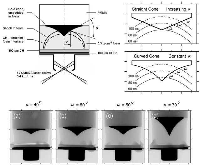
Figure 3: Top left: Laser target design indicating the materials used and scale sizes. The base diameter of the cone is 3 mm. Top right: Depiction of a curved bow shock moving along a straight cone (top) and a curved cone (bottom). The position of the bow shock is shown at sequential times. The intersection angle $\alpha$ increases steadily with time for the straight cone, and is constant for the curved cone. Tick marks are spaced 0.5 mm apart. Bottom: Radiographs of curved cones that produce a constant value of $\alpha$ of (a) 40^∘, (b) and (c) 50^∘, and (d) 70^∘. The serrated cone in panel (c) has a sinusoidal modulation. Tick marks are 1 mm apart.

The design of the laser experiments is summarized in Fig. 3. We used the Omega laser (Soures et al., 1996) at the University of Rochester’s Laboratory for Laser Energetics to drive a strong curved shock through a cylinder of low-density foam within which we embedded a cone-shaped obstacle. In the frame of reference of the intersection point between the curved shock and the cone, the surface of the cone provides a reflecting boundary condition identical to that of two intersecting bow shocks. Hence, our experimental design allows us to explore this intersection point under controlled conditions. The experiments used indirect laser drive to launch the shock wave. Twelve laser beams, each with energy 450 J in a 1 ns pulse, impinge upon the inside surface of a hollow gold hohlraum laser target. The hohlraum had a diameter of 1.6 mm, length 1.2 mm, and laser entrance hole of diameter 1.2 mm. The hohlraum converts the laser energy to thermal X-rays, which subsequently ablate the surface of a composite ablator-pusher that acts as a piston to drive a shock wave into the foam.

We used two types of ablator-pushers. In the first experiments in this series, the ablator was a 100 $\mu$m thick layer of CH doped with 2% by-atom Br with density 1220 mg/cc. This was in contact with a 300 $\mu$m layer of CH (polystyrene) with density 1060 mg/cc that served as a pusher to propel a shock wave into the foam. In later experiments, we changed the design of the ablator-pusher, to reduce radiation preheat of the embedded cone. This design incorporated a 100 $\mu$m thickness CH (polystyrene) ablator and 300 $\mu$m thickness Br-doped CH pusher (6% by-atom Br, 1.5 g/cc density). In all cases, the foam was resorcinol-formaldehyde of density 300 mg/cc. The foam and embedded cone (made from gold, because of its high density) were supported from the end face of a polymethyl methacrylate (PMMA) cylinder of full density.

After a predetermined delay time that ranged from 50 ns to 150 ns to allow the shock wave to propagate to the desired position, the shock wave was imaged by point-projection X-ray radiography along two mutually orthogonal lines of sight, perpendicular to the axis of symmetry of the experimental assembly. The near-point X-ray sources for backlit imaging were provided by using two further laser-illuminated targets, and the images were recorded on a pair of time-gated micro-channel-plate X-ray framing cameras. The output optical images from these cameras were recorded on either photographic film or with a CCD. The laser pulse duration for the x-ray backlighting sources was 600 ps. Contrast in the radiographs is caused by transparency differences through the target, and can be adjusted by altering the composition of the materials. For example, brominated CH absorbs X-rays much more strongly than pure CH foam or plastic do, and will appear correspondingly darker in the radiographs. We used nickel disk laser targets of 400 $\mu$m diameter and 5 $\mu$m thickness as backlighters. These were mounted on 5 mm square, 50 $\mu$m thickness pieces of tantalum sheet. A pinhole of diameter 10 or 20 $\mu$m was machined into the centers of these tantalum supports to aperture x-ray emission from the nickel laser targets, thus providing a near-point X-ray source. A time delay of 7 ns between the two X-ray backlighting laser sources makes it possible to produce two snapshot images, along orthogonal lines of sight and at different times, for each target. The shock velocity through the foam at the position of the cone was typically 20 km s^-1. Radiation preheated the foam to several hundred degrees C before the arrival of the shock, so the preshock sound speed is $\sim$ 1 km s^-1 and the Mach number $\sim$ 20.

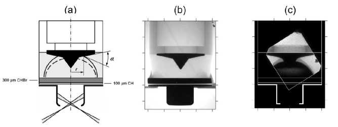
Figure 4: Dual-angle targets. (a) Target design, same as that in Fig. 3, but with dual-cone half angles of 35^∘ and 78^∘. Cones with half angles of 35^∘ and 84^∘ were also used. (b) Target radiograph. (c) Radiograph of the shock as it interacts with the conical surface. The base diameter of the cone is 3 mm and tick marks in (b) and (c) are 1 mm apart. The rectangular area in (c) indicates the diagnostic field of view.

As depicted in Fig. 3, the angle of intersection ($\alpha$) between a curved bow shock and a straight-sided cone that has triangular cross section increases steadily with time, while a curved-sided cone of appropriate form provides a constant angle of intersection. To investigate Mach stem development at a fixed intersection angle we used the concave cone designs shown at the bottom of Fig. 3 for $\alpha$ = 40^∘, 50^∘, 60^∘ and 70^∘. A dual-angled cone like the one shown in Fig. 4 makes it possible to reduce the angle of intersection abruptly to below the critical value, a transition that occurs at a radial distance of 400 $\mu$m or 500 $\mu$m from the cone axis for the targets that we used. Because the dual-angle cones have flat conical cross sections beyond the transition point, $\alpha$ once again increases to greater than the critical angle at later times. Hence, these targets are ideal for investigating the decay and growth rates of Mach stems. A final target design employed a constant incident-angle (50^∘) cone that was ‘terraced’ (panel c in Fig. 3) in order to study the degree to which Mach stems are disrupted by surface irregularities. Terracing of the cone was obtained by machining a sinusoidal modulation onto its surface. Results from these experiments are discussed in §3.3.

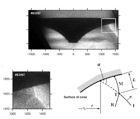
Figure 5: Top: Radiograph of the Mach stem at the surface of the cone. Bottom left: Enlargement of the boxed area. The spatial scale is in $\mu$m. Bottom right: Schematic of the radiographs. T is the triple point between the incident shock (I), reflected shock (R) and Mach stem (M). The incident shock meets the cone at a radial position $r$ and incident angle $\alpha$. The Mach stem size is L.

Figure 5 shows a typical radiograph from the experiment. Our goal is to measure how the length (L) of the Mach stem varies with time. From the experimental data we measure the position and shape of the leading shock wave. We measure the radial position (r), defined as the distance from the axis of symmetry of the bow shock to its intersection with the cone directly from the radiographs (see Yirak et al., 2013). Likewise, the length of the Mach stem is defined in the images as the distance from the location where the Mach stem intersects the surface of the cone to the triple point where the Mach stem, bow shock, and reflected shock meet. We measure the interaction angle $\alpha$ directly from the images.

We attempted several different parameterizations of the profile z = f(r) of the shock wave, and found that the following functional form fits the experimental shape very well:

$$\begin{split}&\theta=ar+br^{2},\\ &{\frac{dz}{dr}}=\tan\theta,\\ &z=z_{\circ}+\int_{0}^{r}\tan(ar+br^{2})dr.\end{split}$$ (2)

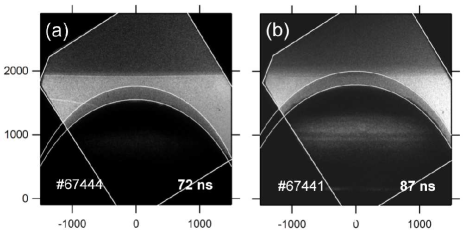
Figure 6: Radiographs (greyscale images) and analytic fits (curved white lines) to the CH(Br)/shocked-foam interface (inner curve) and incident shock front (outer curve) for two experiments. The images were taken at (a) 72 ns and (b) 87 ns. The bow shock moves from the bottom to the top in these images. The boxed area is the diagnostic field of view. Units of the spatial scale are in $\mu$m. The functional form of the analytic fit is given in the text.

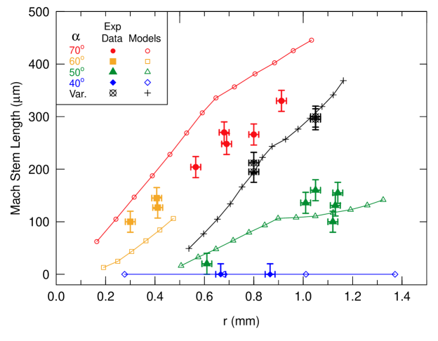
Figure 7: Comparison of PETRA simulations with experimental data of Mach stem growth. Different colors denote curved cones that keep a constant incident angle $\alpha$ with the bow shock. Open symbols denote simulations and filled symbols show experimental measurements. Black points and lines are for a 40^∘ straight cone that has a variable incident angle with the curved bow shock ($\alpha$ = 50^∘ at the apex, increasing to $\sim$ 70^∘ at the edge of the cone). Errorbars depict measurement uncertainties.

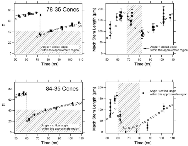
Figure 8: Mach stem destruction and reformation. Top left: The incident angle of the shock as a function of time for the dual-angled cone depicted in panel (b) of Fig. 4. The incident angle drops 11^∘ below the critical value and then rises above it. Open circles depict values from AWE PETRA simulations and solid points with errorbars are experimental data. Dashed-lines are curves fit through the experimental points. Top right: The Mach stem length grows or decays depending on if the angle exceeds the critical value of $\sim$ 42^∘. Bottom: Same as the top panels but for a cone where the angle drops 21^∘ below critical. The Mach stem is destroyed rapidly in this case, but reforms again once the critical angle is reached.

The parameters a and b are approximately independent of time, and z_∘ varies nearly linearly with time. Fig. 6 shows a superposition of this parametric fit on experimental data from targets without an embedded cone. This parameterization of the shock profile was used to define the cone profiles used for the experiments summarized in Fig. 8. For the experiments summarized in Fig. 7, a less-accurate parabolic functional form was used for the shock front and to mill the shape of the concave-sided cones. In consequence, and also because of preheat in the case of these first experiments, the interaction angle is not precisely constant. These issues are discussed in more detail below.

3 Experimental Results

3.1 Mach Stem Growth Rates and Critical Angles

Figure 7 summarizes the Mach stem growth rates for constant intersection angles of 40^∘, 50^∘, 60^∘ and 70^∘. No Mach stems are evident in the 40^∘ data, but Mach stems are present in the 50^∘, 60^∘, and 70^∘ plots. The growth rates increase from zero at 40^∘ to a substantial fraction of the maximum growth rate observed by 50^∘, and remain high at $\alpha$ = 60^∘ and $\alpha$ = 70^∘. The experimental data constrain the critical angle for Mach stem formation $\alpha_{C}$ to lie between 40^∘ and 50^∘, which implies $\gamma$ = 1.31 $-$ 1.56 using Equation 1.

The Eulerian radiation-hydrodynamical code PETRA (Youngs, 1984) was used to simulate our experiments. Eulerian hydrodynamics is essential to treat the large shear flows over the surface of the gold cones, and the simulations included the full foil-foam-cone package and the laser-heated hohlraum, represented on a fixed 1.25 $-$ 2.5 $\mu$m-resolution mesh. X-ray diffusion was used to drive the hohlraum evolution and the acceleration of the ablator-pusher foil. Most of the equations-of-state were taken from the LANL SESAME library (Holian, 1984). Mach stem lengths for each numerical model in Fig. 7 are connected by lines, and fit the experimental data reasonably well. Differences between the models and experimental data for the 60^∘ and 70^∘ cones likely arise from two complications. First, the radiographs from the experiments completed early in the campaign show that the cone began to ablate before the arrival of the bow shock owing to radiative pre-heating. These effects, not included in the numerical simulations, were reduced in the later experiments by using a pusher designed to be more opaque to radiation (Sec. 2). The second complication is that while the curved cones were designed to maintain as constant of an incident angle as possible, some variation does occur in this angle as the bow shock evolves. In the numerical simulations we found that $\alpha$ maintained the desired value to within $\sim$ $\pm$ 4^∘. Variations of this order, combined with the effects of radiative preheating, are the most likely cause of the differences between models and experiments in Fig. 7. Simulations of the potentially more-complex case of a straight cone with a variable incident angle agree with the experimental data within the uncertainties.

Because the numerical results reproduce the experimental data well, we can use the simulations to narrow the uncertainties of experimental $\gamma$ considerably. Models and experimental data for the dual cones (Sec. 3.2) show positive growth rates when $\alpha$ $\gtrsim$ 42^∘ $\pm$ 1^∘. With this range for $\alpha_{C}$ we find $\gamma$ = 1.49 $\pm$ 0.03 from Eqn. 1. As a check of the validity of the analytical values, AstroBEAR models with $\gamma$ = 1.4 of dual bow shocks described in section 4.1 yield $\alpha_{C}$ = 43^∘, which, using Eqn. 1, would imply $\gamma$ = 1.47, a value 5% higher than the actual one. If we apply this 5% correction to our numerical and experimental value of $\gamma$ = 1.49, we obtain $\gamma$ = 1.42 for the experimental $\gamma$, with an observational uncertainty of $\sim$ 2%, and a systematic uncertainty in translating $\alpha_{C}$ to $\gamma$ of $\sim$ 5%. The experimental value of $\gamma$ is considerably lower than that of an ideal monatomic gas (5/3). Some energy from the shock goes into completing the vaporization of the foam that was begun by the radiative preheating, and more energy losses occur from dissociating and ionizing the resultant CH gas. These processes lower $\gamma$ from the monatomic gas result.

3.2 Experiments of Mach Stem Regrowth and Hysteresis

Depending in part on whether or not $\alpha$ exceeds the critical value, Mach stems should either grow, remain stationary with time, or decay. In the parlance of Ben-Dor (2007), these three cases are referred to as direct, stationary, and inverse Mach reflection, respectively. Dual-angled cones such as the one shown in panel (b) of Fig. 4 have the desirable property that the incident angle steadily increases, then decreases sharply to below the critical angle, and finally increases again to greater than the critical angle, making it possible to study how the Mach stem responds to sudden changes in the intersection angles. However, as we investigate numerically in Sec. 4.1.1, growth rate is not determined uniquely by $\alpha$ in all cases, but also depends upon the hydrodynamical flow present in the postshock region.

Figure 8 summarizes results from the dual-angled cone experiments. We constructed two types of dual-angled cones, a set of ‘78-35’ targets where the intersection angle dropped below $\alpha_{C}$ by $\sim$ 11^∘, and a set of ‘84-35’ targets that dropped below $\alpha_{C}$ by $\sim$ 21^∘. The shaded region in Fig. 8 depicts the subcritical angle regime $\alpha$ $<$ $\alpha_{C}$ for the two cases. In both types of targets, the Mach stem decays in size as soon as the intersection angle becomes subcritical. The decay is rapid for the 84-35 targets and the Mach stem disappears. However, the Mach stem is not destroyed immediately in the 78-35 targets, and for both types of targets the Mach stem once again grows as soon as $\alpha$ $\gtrsim$ 42^∘, which we take to be the critical angle $\alpha_{C}$. The top-right panel of Fig. 8 shows that the decay and growth rates on either side of the critical angle are similar.

As noted in the Introduction, Mach stems exhibit hysteresis phenomena in the sense that the critical angle of transition from RR to MR differs from that of MR to RR. Our dual-angled cones cross the critical angle both from the MR regime into RR, where decay is observed, and from RR into MR, where growth occurs. However, as these experiments are time-dependent, they do not test Mach stem formation and destruction as intersection angles are varied in a quasi-static manner across the critical values, a regime where wind-tunnel experiments are more optimal. The critical angles in the targets where $\alpha$ varies rapidly with time are (within the measurement uncertainties) the same as those inferred from the targets that have constant $\alpha$. The critical angle for decay is much less-constrained: the data only imply that 11^∘ subcritical suffices to initiate decay, and that the decay occurs more rapidly at 21^∘ subcritical.

3.3 Experiments and Models of Mach Stem Survival Along Inhomogeneous Surfaces

Once a Mach stem grows larger than any surface irregularities, its triple point should flow over the top of the irregularities. However, the situation when the surface irregularities are larger than the triple point is less clear, especially early in the growth stage when the Mach stem is small. When $\alpha$ $<$ $\alpha_{C}$ we expect the Mach stem to decay, and for this case Ben-Dor & Takayama (1986) showed inverse Mach reflection (i.e. Mach stem decay) proceeds steadily and the triple point lowers to the surface. After the triple point contacts the surface, the system readjusts to a new configuration known as transitioned regular reflection (TRR) characterized by a leading RR followed by a Mach reflection.

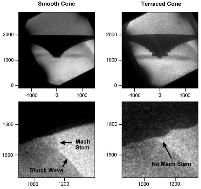
Figure 9: Mach stems and irregular surfaces. Left: The radiograph shows a well-defined Mach stem where the shock wave meets the surface of the smooth cone. The laser drives a shock wave from the bottom to the top. Right: A similar cone with a terraced surface does not produce a Mach stem. Axis labels are distances in $\mu$m.

To investigate this case experimentally, we constructed a terraced cone from a constant-incident angled 50^∘ cone as depicted in Fig. 9. As shown in the figure, a prominent Mach stem exists by the time the bow shock has traversed the smooth 50^∘ cone, while the terraced cone shows no Mach stem. The simplest explanation for the lack of a Mach stem for the terraced cone is that any Mach stem that may form does not grow fast enough to allow the triple point to clear the next terrace. Combined with data in the previous section, this result implies that although Mach stems can survive sudden and erratic changes in the intersection angles, they are easiest to create when conditions are relatively smooth.

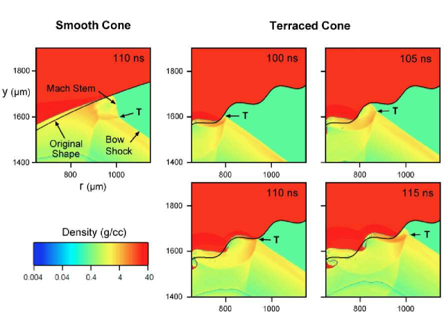
Figure 10: PETRA simulations of the bow shock moving along the surface of a smooth cone (left), and a terraced cone (right). The curved surface of the cone keeps a constant angle of 50^∘ between the bow shock and the cone’s surface. The point marked ‘T’ is the triple point. The Mach stem grows in the valleys and is destroyed in the hills of the terraced cone, but grows steadily along the smooth cone. Scale sizes are the same as those in Fig. 9, and the times in ns after the laser pulse are shown for each panel.

Numerical models in Fig. 10 illustrate this phenomenon. After 110 ns a well-defined Mach stem has formed along the surface of the smooth cone. In contrast, while a Mach stem grows quickly in the valleys of the terraced cone, the triple point (labeled ‘T’ in Fig. 10) runs into the top of the next ridge as the bow shock proceeds. Hence, the surface irregularities are large enough to inhibit Mach stem growth in this case. We see no clear evidence for TRR, but the situation is far from steady-state and the spatial resolution of the simulations may need to be higher to resolve this feature.

4 Physics of Mach Stem Evolution and its Astrophysical Implications

Why do Mach stems form? As described in the Introduction and depicted in Fig. 1, a triple point is sometimes needed to satisfy the boundary conditions when two shocks intersect. Interpretations that involve more physical insight are discussed in detail by Ben-Dor (2007). One school of thought is that the critical angle $\alpha_{C}$ for Mach stems is set when the gas behind the reflected shock becomes subsonic (e.g. von Neumann, 1943). Another point of view is that the critical angle occurs when the compression behind the reflected shock matches that of a normal bow shock, which would allow a Mach stem to grow without a sudden pressure change (Hendersen & Lozzi, 1975). Ben-Dor (2007) remarks that the supersonic criterion appears to be the one best supported by experimental data.

4.1 Minimum and Maximum Critical Angles for Intersecting Bow Shocks

We conducted a series of numerical simulations in order to clarify how Mach stems form, evolve, and dissipate when they result from intersecting bow shocks. The simulations were done with the AstroBEAR code in 2-D (planar symmetry). AstroBEAR is a fully 3-D MHD parallelized code with adaptive mesh and cooling capabilities (Cunningham et al., 2009; Carroll-Nellenback et al., 2012). The setup used gases with fixed $\gamma$ = 1.67, 1.4 and 1.2, and Mach numbers M = 1.6, 5.2, and 30. These parameters are shown alongside the experimental and observational values in Table 1.

In the numerical models, two circular obstacles with diameters of d_∘ = $3\times 10^{14}$ cm were embedded into a 50 km s^-1 wind, and for each of the nine combinations of $\gamma$ and M, the simulation followed the evolution for $\sim$ 40 $\tau_{F}$, where the flow time $\tau_{F}$ = 1.9 years is defined as the time it takes unperturbed wind to move one obstacle diameter. The density of the wind was $5\times 10^{3}$ cm^-3, and the initial density contrast was $2\times 10^{3}$ between the obstacles and the incident flow. We also investigated a model with a higher-density contrast of $2\times 10^{5}$ to assess how much deformations in the obstacles affected the results.

4.1.1 Numerical Simulations for $\gamma$ = 1.4 and M = 5.2

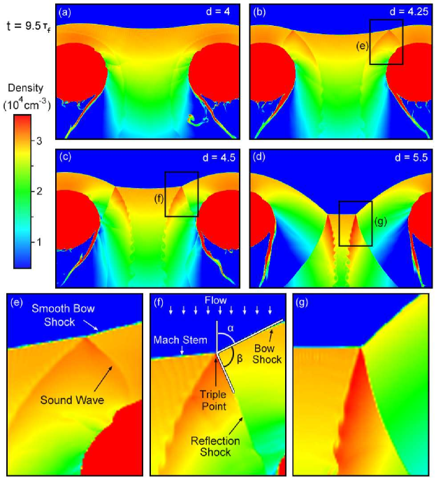
Figure 11: Top and Middle: AstroBEAR 2-D simulations for $\gamma$ = 1.4 and M = 5.2 of intersecting bow shocks at t = 9.6$\tau_{F}$, where $\tau_{F}$ is the time it takes for the unperturbed flow to traverse the diameter of the obstacle. The colors denote different densities. The parameter d refers to the initial separation between the obstacles in units of the obstacle radius. Bottom: Expansion of the boxed regions around the triple points. The angles $\alpha$ and $\beta$ are discussed in the text.

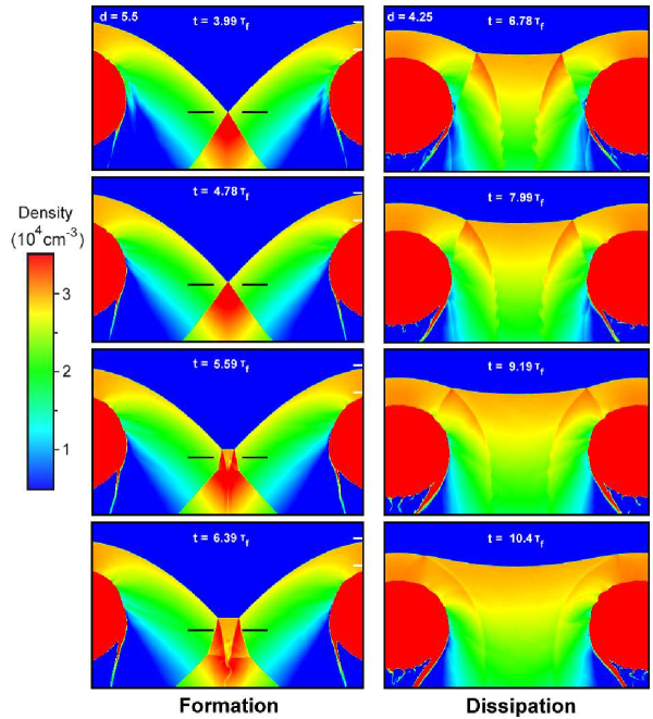
Figure 12: Left: Density plots of the time-evolution of the triple point in the d = 5.5 r_∘ case shown in Fig. 11, which begins as regular reflection and develops a Mach stem. Black fiducials mark the initial location of the triple point, and white fiducials mark the initial locations of the bow shock and obstacle boundary. Right: Time-sequence of the triple point for d = 4.25 r_∘. As the system approaches, and then exceeds $\alpha_{M}$, the reflection shocks become sound waves, the triple point dissipates, and the bow shock becomes smooth. The color scale is the same as those in Fig. 11.

The $\gamma$ = 1.4 simulations with M = 5.2 are summarized in Figs. 11 and 12. At any given time, the simulations exhibit one of three configurations determined primarily by the separation between the obstacles and the amount of time the system has had to evolve: (i) regular reflection where the bow shocks meet, (ii) a Mach stem between the bows, or (iii) a single smooth shock that encompasses both obstacles. For the $\gamma$ = 1.4 models, when the obstacle separation d $\gtrsim$ 6 r_∘ (r_∘ is the obstacle radius) the intersection angle $\alpha$ between the bow shocks is below the critical angle $\alpha_{C}$, and the system shows regular reflection for the length of the simulation. If the obstacles are close enough that $\alpha$ is not too far below $\alpha_{C}$ (e.g. Model d = 5.5 r_∘ in Fig. 12), the incident angle $\alpha$ may grow enough with time to exceed $\alpha_{C}$ at some point, which causes a Mach stem to form after an initial period of regular reflection (left panels of Fig. 12). Both the d = 5.5 r_∘ and d = 5.0 r_∘ models settle into a quasi-steady-state configuration with a stable Mach stem at later times. In addition to the triple point where the Mach stem, bow shock and reflection shock meet, there is also a contact discontinuity that marks the boundary between gas that enters the Mach stem and gas that goes through the bow shock and then the reflection shock. This contact discontinuity shows a significant amount of Kelvin-Helmholtz growth in the simulations.

Mach stems that occur at smaller separations (d $\lesssim$ 4.5 r_∘) grow steadily with time as the location of the intersection point between the bow shocks moves upstream, raising $\alpha$. As $\alpha$ approaches 90^∘ and the triple point moves closer to the apices of the bow shocks, the bow shocks redirect postshock material towards the triple point as they do when $\alpha$ is smaller, but at a lower velocity relative to the triple point. Once the motion of the postshock gas relative to the reflection shock becomes subsonic, the reflection shock becomes a sound wave, and the numerical simulations show that the Mach stem merges with the bow shock to produce a single curved shock around the obstacles. This behavior is shown in the right panels of Fig. 12. Hence, there is a maximum angle $\alpha_{M}$ above which the triple point and the Mach stem disappear and are replaced by a smoothly-varying bow shape.

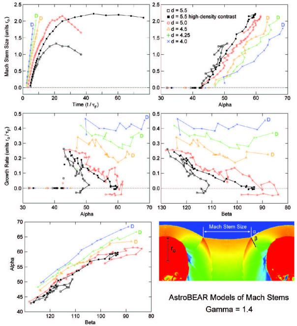
Figure 13: AstroBEAR models of intersecting bow shocks for $\gamma$ = 1.4 and M = 5.2. Top: Mach stem size as a function of time and of the incident angle $\alpha$ defined in the lower right panel. The radius of the obstacles is r_∘ and the time for the preshock gas to flow past the obstacle is $\tau_{F}$. The largest Mach stems have size $\sim$ 2 r_∘. The symbol ‘D’ indicates where the Mach stem dissipated as it became subsonic. Middle: Mach stem growth rates as a function of the angles $\alpha$ and $\beta$. Growth rates that drop to zero imply stable Mach stems. Bottom: Relationship of $\alpha$ to $\beta$ in the models.

Our numerical models indicate that Mach stems only survive as long as the angle $\beta$ between the bow shock and the regular reflection shock at the triple point exceeds $\sim$ 90^∘ (Fig. 13). The maximum diameter of a Mach stem in the simulations is $\sim$ 2 r_∘. For these transient Mach stems, as $\alpha$ increases, $\beta$ decreases, and when $\beta$ falls below $\sim$ 90^∘ the lateral motion into the reflection shock becomes subsonic, and the wave detaches from the bow, which is now a smoothly-varying curved surface. Models with smaller separations exhibit higher growth rates and evolve into a single bow shock more quickly (Figs. 11 and 13).

The value of $\alpha_{M}$ ranges between 62^∘ and 68^∘ in our $\gamma$ = 1.4, M = 5.2 simulations for the different values of initial obstacle separation. The precise value depends upon how much the Mach stem is curved, which alters the angles at the triple point. Mach stems with more widely-separated obstacles curve more, and the curvature is also influenced by how rapidly the flow destroys the obstacles. In all cases, detachment of the triple point from the bow shock begins when $\beta$ $\lesssim$ 90^∘. Hence, transient Mach stems form and grow over a range of $\alpha$ $\sim$ 20 $-$ 25 degrees, and eventually result in a single smooth shock on timescales that range from a few obstacle crossing times, to an order of magnitude higher than this value. In the d = 5.5 r_∘ and d = 5 r_∘ models, the Mach stem remained in quasi-static equilibrium for the entire length of the simulation ($\sim$ 40 crossing times).

The high-density-contrast model with d = 5.5 r_∘ (filled black squares in Fig. 13) resembles that of the lower-density contrast models d = 5.5 r_∘ at early times, and d = 5.0 r_∘ at later times. Obstacles in the lower-density contrast model are more affected by compression and undergo more mass stripping from the wind. However, the effects of changing the density contrast are minor compared with changing the separation, evolution time, $\gamma$, and Mach number (see below).

4.1.2 Numerical simulations for other values of $\gamma$ and the Mach number M

Our simulations with different values of $\gamma$ and M follow the same pattern as those for $\gamma$ = 1.4 and M = 5.2 described above. At early times, systems where the object separations are small show individual bow shocks and a Mach stem. At later times, these shocks grow to form a single curved shock that encompasses both obstacles. No Mach stems form at when the obstacle separations are large, while stable Mach stems exist at intermediate separations.

We measured the critical angle $\alpha_{C}$ for Mach stem formation in each combination of $\gamma$ and M, and compile these results in Table 2. The last columns in the Table show the predicted values of $\alpha_{C}$ in the limit of infinite M for both the Courant & Friedrichs (1948) formalism (Equation 1) and from Equation 6 of De Rosa et al. (1992). Both analytic equations explain the simulation results reasonably well for $\gamma$ = 1.67 and 1.4, but the De Rosa et al. (1992) equation matches much better at $\gamma$ = 1.2. The critical angle increases as the Mach number approaches unity for all values of $\gamma$.

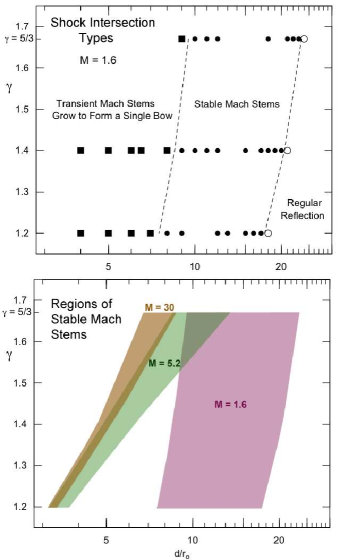
Figure 14: Top: Mach stem behavior after 40 dynamical timescales for 2-D AstroBEAR simulations with Mach number = 1.6, as a function of the polytropic index $\gamma$ and the logarithm of the separation d between two cylindrical obstacles of radius r_∘. Squares are transient Mach stems, filled circles are stable Mach stems, and open circles are regular reflections. Bottom: Ranges of stable Mach stems as a function of the polytropic index $\gamma$, the obstacle separation d/r_∘, and the Mach number M. Stable Mach stems form most readily with larger $\gamma$ and smaller M.

The range of separations that allow stable Mach stems to form depends upon both $\gamma$ and M. The top panel of Fig. 14 shows that stable Mach stems exist for larger obstacle separations and persist over a wider range of distances when $\gamma$ is larger. For example, when M = 1.6, stable Mach stems exist after 40 $\tau_{F}$ when 7.5 $\lesssim$ d/r_∘ $\lesssim$ 17.5 for $\gamma$ = 1.2, 8.5 $\lesssim$ d/r_∘ $\lesssim$ 20.5 for $\gamma$ = 1.4, and 9.5 $\lesssim$ d/r_∘ $\lesssim$ 23.5 for $\gamma$ = 5/3. At smaller separations, transient Mach stems grow to encompass both obstacles, and at larger separations the bow shock wings intersect with regular reflection. In all cases, the maximum Mach stem diameter is $\sim$ 2 r_∘. The bottom panel of Fig. 14 shows that increasing the Mach number narrows the range of distances that produce stable Mach stems, and also moves this range to smaller separations.

We can understand the dependence of stable Mach stems on $\gamma$ and M by considering the dynamics of the postshock gas. As $\gamma$ decreases, the postshock pressure declines and bow shocks wrap more closely around obstacles. For the case of two obstacles considered here, it means that the obstacles must lie closer together for the intersection angle to exceed the critical value to form a Mach stem. Similarly, when the preshock temperature declines, increasing M, the postshock pressure is less important dynamically and bow shocks also wrap more closely around the obstacles. Both effects appear in the bottom panel of Fig. 14. The effect of the postshock pressure on the shape of bow shocks has been known for several decades, for example, in numerical simulations of cooling jets where a dense plug forms around the jet at the leading working surface (Blondin et al., 1990). The most extreme case is that of an isothermal shock ($\gamma$ = 1), where cooling to preshock temperatures occurs immediately behind the shock, and no Mach stems form.

4.2 Possible Astrophysical Examples

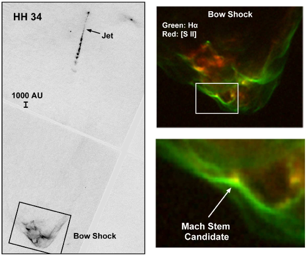
Figure 15: Candidate Mach stem within an astronomical outflow. Left: HST image of the young stellar jet HH34 and its bow shock (from (Hartigan et al., 2011)). Right: Expanded views of the bow shock and the putative Mach stem.

From an astrophysical standpoint, Mach stems are potentially important because they change the geometry of shock intersections from oblique to normal, and can produce a quasi-static or transient ‘hot spot’ of enhanced emission and excitation at this location. A prime candidate for this phenomenon exists in the bow shock of the HH 34 stellar jet (Hartigan et al., 2011). Figure 15 shows that a bright emission knot exists immediately behind the intersection point of two arc-shaped shocks. This knot, as well as several others in this object, have anomalous proper motions that do not follow along with the bulk motion of the bow shock. Anomalous pattern motion is expected if the proper motions simply trace the location of the shock intersection points.

The structured bow shock in HH 47 (Hartigan et al., 2011) is another potential example where transient Mach stems may occur. This object resolves into what appear to be dozens of small knots in high-resolution images. Surprisingly, these bright points form and dissipate on timescales of a decade, which is difficult to explain if they represent discrete knots of high density that plow through the working surface of the flow. In both HH 34 and HH 47, the shock velocity is $\sim$ 100 km s^-1 and the knot size $\sim$ 7.5$\times 10^{14}$ cm, so $\tau_{F}$ $\sim$ 2.4 years. The numerical models imply we should expect any transient Mach stems to evolve on a timescale of about a decade, in agreement with the observations.

The postshock regions of cooling astrophysical shocks are complex, and contain various zones of ionization for each element, so these regions are not characterized by a single value of $\gamma$. However, the overall dynamical effects of cooling in bow shocks has been well-established for some time (e.g. Blondin et al., 1990). A critical parameter is the ratio of the cooling-zone distance d_COOL to the obstacle size d_∘. When this ratio is $\gtrsim$ 1, the gas acts like an adiabatic flow with $\gamma$ = 5/3, where the maximum size of a Mach stem will be comparable to d_∘. In the opposite limit when the obstacle is very large compared with the cooling length, the gas behaves dynamically as if it is isothermal. An isothermal shock has $\gamma$ = 1, where no Mach stems are possible. In this case, Mach stems only exist on scale sizes $\lesssim$ d_COOL. Hence, the maximum size of a Mach stem should be the smaller of d_COOL or d_∘. The cooling distance scales inversely as the preshock density and directly as a power of the shock velocity (e.g. Hartigan et al., 1987), and also depends upon the strength of the magnetic field (Hartigan and Wright, 2015). Hence, whether or not two intersecting bow shocks create a substantial Mach stem depends upon the shock velocity, density, magnetic field strength, as well as the size of the bows. Overall, Mach stems should be most common when size scales are small enough to render cooling unimportant in the dynamics.

The distribution of clumps in the flow and ambient medium ultimately determines whether or not Mach stems will form and grow in any situation, with the optimal separation for Mach stem growth being several times the diameter of the obstacles in a flow with moderate Mach number. The widest range of allowable obstacle separations occurs when cooling is least important (Sec. 4.1.2). Cooling distances in the HH 34 and HH 47 bow shocks are on the order of the size of the transient bright knots in these objects (Hartigan et al., 2011). Hence, the effective $\gamma$ for these spatial scales is $\sim$ 5/3, favorable for Mach stem growth. We present simulations of intersecting shocks in 3-D, driven by velocity-variable jets with accurate radiative emission-line cooling in a future paper (Hansen et al., 2016, submitted to ApJ).

5 Summary

In this paper we examined hydrodynamical phenomena associated with Mach stems, which are normal shocks that occur whenever two shock waves intersect one another within a certain range of angles. Using the Omega laser facility we created Mach stems in high-Mach number plasmas under controlled conditions in the laboratory with cone-shaped targets, and complemented this work with numerical simulations of the experiment and for the more astrophysically-relevant case of intersecting bow shocks. Our main focus has been to understand how Mach stems respond as the angle between the two incident shocks (equivalently, the angle between the shock wave and a surface) varies in supersonic plasmas.

Our first set of experiments employed a design that enforced a constant angle between a curved shock and a conical surface. These experiments demonstrated that the Mach stem growth rate was highest for the largest incident angles and the rate increased most rapidly when the intersection angle was closer to the critical value $\alpha_{C}$. The measured value of $\alpha_{C}$ from the constant-angle cones was between 40^∘ and 50^∘. Experiments with dual-angled cones allowed for a more precise estimate of $\alpha_{C}$, as well as a means to quantify Mach stem decay rates when $\alpha$ $<$ $\alpha_{C}$. After using the experimental growth rate to verify simulations of the experiment, we combined the simulations and experimental data together to refine the critical angle $\alpha_{C}$ in the experiments to 42^∘ $\pm$ 1.0^∘. Numerical simulations with different values of $\gamma$ and the Mach number M made it possible to test analytical formulae that translate $\alpha_{C}$ to $\gamma$, and we found that the relatively simple formula from Courant & Friedrichs (1948) reproduces the numerical results with approximately a 5% error as long as $\gamma$ $\gtrsim$ 1.4. At smaller values of $\gamma$, only the more complex analytic formula for $\alpha_{C}$ from De Rosa et al. (1992) is consistent with the simulations. Our best estimate for the effective $\gamma$ of the shocked foam is $\sim$ 1.42. This value differs significantly from the ideal monatomic gas $\gamma$ of 5/3 owing to the energy lost to dissociation and ionization of the gas once the solid has been vaporized.

Simple geometrical considerations argue that Mach stems should dissipate between intersecting bow shocks if the stems grow too large, and our numerical simulations confirm this hypothesis. When the angle between the bow shock and the outer reflection shock becomes acute, the reflection shocks at the triple point become subsonic, and the triple point dissipates as the Mach stem joins smoothly with the main bow shocks. The critical incident angle at which this occurs depends upon the curvature of the Mach stem, and ranges between 62^∘ and 68^∘ for $\gamma$ = 1.4. Hence, there is a range of incident angles of $\sim$ 25 degrees over which Mach stems occur.

Bow shocks that intersect produce one of four outcomes: (i) steady-state regular reflection, (ii) transient regular reflection that evolves into a Mach stem, (iii) a steady-state Mach stem, or (iv) a transient Mach stem that grows to envelop both obstacles and produce a single smooth shock at late times. As the separation between the obstacles decreases, systems transition from cases (i) and (ii) to cases (iii) and (iv). The range of separations that produce Mach stems is higher for larger $\gamma$ and lower Mach numbers. The maximum size for a Mach stem is comparable to the diameter of the obstacles, and the characteristic lifetimes for most transient Mach stems are $\sim$ 10 flow times.

Our experiments show that Mach stems persist in high-Mach number plasma shocks, and are relatively robust in the sense that when the intersection angle drops below the critical value the Mach stems decay but are not destroyed immediately. The decay rate in the size of the Mach stem at subcritical angles appears comparable to the growth rates for supercritical angles. In our experiments, after a sudden decrease of the intersection to subcritical, the angle gradually rose until it once again exceeded the critical value, after which the Mach stem again grew. In real astrophysical situations the ambient medium can be highly nonuniform, resulting in bumpy shock fronts. Our experiments show that a rough surface can inhibit Mach stem growth if the Mach stem does not grow fast enough to flow past the surface irregularities. Simulations with $\gamma$ = 1.2 and $\gamma$ = 5/3 show that cooling also significantly inhibits Mach stem growth, so that Mach stems are most likely to form on size scales $\lesssim$ d_COOL.

Despite these restrictions, there is some observational evidence for Mach stems in an astrophysical context. Mach stems are an attractive explanation for the bright knots in the HH 34 bow shock, both from the standpoint of morphology and from anomalous pattern motions that appear to trace intersection points between distinct bow shocks. Transient bright knots in the HH 47 bow shock may also arise from Mach stems. The timescales for the appearance of these knots are consistent with those predicted by the numerical models. Hence, Mach stems are likely to occur in a variety of astrophysical situations that involve intersecting shocks, though the Mach stem sizes will not be larger than the diameter of the obstacles that produce the bows, and stems only form readily when the obstacles are smaller than the cooling distance behind the shocks. As a result, most astrophysical Mach stems will be difficult to resolve spatially.

More complex numerical simulations should give further insights into Mach stem formation and decay. Relaxing the 2-D symmetry of the simulations will greatly increase the geometrical possibilities, and will likely reduce the area of Mach stems in most systems. An interesting case to model would be when one bow shock overtakes another, as Mach stems should form over a range of times centered near where the faster bow overtakes the slower one. Another issue is to consider the role magnetic fields may play in the phenomenon. Magnetic fields oriented perpendicular to the flow will become bent as the flow drags them into the intersection points between shocks, and the resulting tension force will provide some back pressure that should enhance Mach stems as they lower the Alfvénic Mach numbers. Magnetic fields also lengthen cooling zones, which should raise the effective $\gamma$ of the system and make it easier for Mach stems to form over larger size scales. Whether or not the geometry and cooling of a given object permit Mach stems to form, intersection points of shocks are natural locations for density enhancements and time-variability in clumpy supersonic flows.

Figure 1: Geometry of intersecting bow shocks. Left: When the angle of intersection $\alpha$ is smaller than a critical value that depends on the specific heat ratio $\gamma$ of the gas, regular reflection occurs and a single reflected shock follows in the wake of the intersection point. Right: As the apices of the bow shocks approach one-another, the system transitions to Mach reflection, and the intersection point becomes a normal shock known as a Mach stem.

References

- Anderson et al. (1994) Anderson, M. C., Jones, T. W., Rudnick, L., Tregillis, I. L., & Kang, H. 1994, ApJ, 421, L31
- Ben-Dor & Takayama (1986) Ben-Dor, G. & Takayama, K., 1986/7, “The dynamics of the transition from Mach to regular reflection over concave cylinders”, Israel J. Tech., 23, 71–74
- Ben-Dor (2007) Ben-Dor, G. 2007, Shock Wave Reflection Phenomena, 2nd ed. (Berlin:Springer)
- Ben-Dor et al. (2002) Ben-Dor, G., Ivanov, M., Vasilev, E., & Elperin, T. 2002, Progress in Aerospace Sciences, 38, 347
- Blondin et al. (1990) Blondin, J.M., Fryxel, B.A., & Königl, A. 1990, ApJ 360, 370
- Carroll-Nellenback et al. (2012) Carroll-Nellenback, J., Shroyer, B., Frank, A., & Ding, C. 2012, in Numerical modeling of space plasma flows, N.V. Pogorelov, J.A. Font, E. Audit, and G.P. Zank eds., (San Francisco: Astronomical Society of the Pacific), ASP Conf. Ser. Vol. 459, p291
- Chevalier & Theys (1975) Chevalier, R. A., & Theys, J. C. 1975, ApJ, 195, 53
- Chpoun et al. (1995) Chpoun, A., Passerel, D., Li, H., & Ben-Dor, G. 1995, J. Fluid Mech. 301, 19
- Courant & Friedrichs (1948) Courant, R., & Friedrichs, K. O. 1948, Supersonic Flow and Shock Waves in Applied Mathematical Sciences Vol. 21 (Berlin:Springer).
- Cunningham et al. (2009) Cunningham, A.J., Frank, A., Varniere, P., Mitran, S., & Jones, T.W. 2009, ApJS 182, 519
- De Rosa et al. (1992) De Rosa, M., Fama, F., Palleschi, V., Singh, D.P. & Vaselli, M. 1992, Phys. Rev. A 45, 6130
- Foster et al. (2010) Foster, J. M., Rosen, P. A., Wilde, B. H., Hartigan, P., & Perry, T. S. 2010, Physics of Plasmas, 17, 112704
- Hartigan et al. (2011) Hartigan, P., Frank, A., Foster, J. M., Wilde, B., Douglas, M., Rosen, P., Coker, R., Blue, B., & Hansen, F. 2011, ApJ, 736, 29
- Hartigan et al. (2001) Hartigan, P., Morse, J. A., Reipurth, B., Heathcote, S., & Bally, J. 2001, ApJ, 559, L157
- Hartigan et al. (1987) Hartigan, P., Raymond, J.C., & Hartmann, L. 1987, ApJ 316, 323
- Hartigan and Wright (2015) Hartigan, P., & Wright, A. 2015, ApJ 811, 12
- Hendersen & Lozzi (1975) Hendersen, L.F. & Lozzi, A. 1975, J. Fluid Mech. 68, 139
- Holian (1984) Holian, K.S. 1984, “T-4 handbook of material properties data bases. Vol Ic: Equations of state”, Los Alamos National Laboratory Report No. LA-10160-MS
- Hu & Glass (1986) Hu, T.C.J., & Glass, I.I. 1986, AIAA Journal 24, 607
- Kawamura & Saito (1956) Kawamura, R. & Saito, H. 1956, J. Phys. Soc. Japan, 11, 584
- Li & Ben Dor (1996) Li, H., & Ben Dor, G. 1996, J. Appl. Phys 80(4) 2027
- Shara et al. (1997) Shara, M. M., Zurek, D. R., Williams, R. E., Prialnik, Gilmozzi, & Moffat 1997, AJ 114, 258
- Soures et al. (1996) Soures, J.M., et al. 1996, Phys. Plasmas 3, 2108
- White (1951) White, D.R., 1951, “An experimental survey of the Mach reflection of shock waves”, Princeton Univ., Dept. Phys., Tech. Rep. II-10, Princeton, N.J., USA.
- von Neumann (1943) von Neumann, J. 1943, “Oblique reflection of shocks”, Explos. Res. Rep. 12, Navy Dept., Bureau of Ordinance, Washington, DC, USA
- Yirak et al. (2013) Yirak, K. et al. 2013, High Energy Density Phys. 9, 251
- Youngs (1984) Youngs, D.L. 1984, Physica D 12, 32