Towards Practical Bayesian Parameter and State Estimation

Abstract

Joint state and parameter estimation is a core problem for dynamic Bayesian networks. Although modern probabilistic inference toolkits make it relatively easy to specify large and practically relevant probabilistic models, the silver bullet—an efficient and general online inference algorithm for such problems—remains elusive, forcing users to write special-purpose code for each application. We propose a novel blackbox algorithm – a hybrid of particle filtering for state variables and assumed density filtering for parameter variables. It has following advantages: (a) it is efficient due to its online nature, and (b) it is applicable to both discrete and continuous parameter spaces . On a variety of toy and real models, our system is able to generate more accurate results within a fixed computation budget. This preliminary evidence indicates that the proposed approach is likely to be of practical use.

1 Introduction

Many problems in scientific studies and natural real-world applications involve modelling of dynamic processes, which are often modeled by dynamic probabilistic models (DPM) (Elmohamed et al., 2007; Arora et al., 2010). Online state and parameter estimation –computing the posterior probability for both (dynamic) states and (static) parameters, incrementally over time– is crucial for many applications such as simultaneous localization and mapping, real-time clinical decision support, and process control.

Various sequential Monte-Carlo state estimation methods have been introduced for real-world applications (Gordon et al., 1993; Arulampalam et al., 2002; Cappé et al., 2007; Lopes & Tsay, 2011). It is yet a challenge to estimate parameters and state jointly for DPMs with complex dependencies and nonlinear dynamics. Real-world models can involve both discrete and continuous variables, arbitrary dependencies and a rich collection of nonlinearities and distributions. Existing algorithms either apply to a restricted class of models (Storvik, 2002), or are very expensive in time complexity (Andrieu et al., 2010).

DPMs in real-world applications often have a large number of observations and one will need a large number of particles to perform the inferential task accurately, which requires the inference engine to be efficient and scalable. While there is much success in creating generic inference algorithms and learning systems for non-dynamical models, it remains open for DPMs. A black-box inference system for DPMs needs two elements to be practically useful: a general and effective joint state/parameter estimation algorithm and an efficient implementation of inference engine. In this paper, we propose a practical online solution for the general combined state and parameter estimation problem in DPMs. We developed State and Parameter Estimation Compiler (SPEC) for arbitrary DPMs described in a declarative modelling language BLOG (Milch et al., 2005). SPEC is equipped with a new black box inference algorithm named Assumed Parameter Inference (API) which is an hybrid of particle filtering for state variables with assumed density filtering for parameter variables. SPEC is also geared with an optimizing compiler to generate application specific inference code for efficient inference on real-world applications.

Our contribution of the paper is as follows: (1) We proposed a new general online algorithm, API, for joint state and parameter estimation, regardless whether the parameters are discrete or continuous, and whether the dynamics is linear or nonlinear; (2) We developed a black box inference engine, SPEC, equipped with API for arbitrary DPMs. SPEC also utilizes modern compilation techniques to speedup the inference for practical applications; (3) We conducted experiments and demonstrated SPEC’s superior performance in terms of both accuracy and efficiency on several real-world problems.

We organize the paper as follows: Section 2 reviews the state and parameter estimation literature, section 3 describes our new algorithm API, and introduces our black box inference engine SPEC, and section 4 provides experiment results. Further discussion is given in section 5. Finally we conclude our paper in section 6.

2 Background

An overview of SMC methods for parameter estimation is provided in (Kantas et al., 2015). Plain particle filter fails to estimate parameters due to the inability to explore the parameter space. This problem is particularly severe in high-dimensional parameter spaces, as a particle filter would require exponentially many (in the dimensionally of the parameter space) particles to sufficiently explore the parameter space. Various algorithms have been proposed to achieve the combined state and parameter estimation task, however, the issue still remains open as existing algorithms either suffer from bias or computational efficiency. The artificial dynamics approach (Liu & West, 2001), although computationally efficient and applicable to arbitrary continuous parameter models, results in biased estimates and fails for intricate models considered in this paper. The resample-move algorithm (Gilks & Berzuini, 2001) utilizes kernel moves that target $p(\theta,x_{0:t}\mid y_{0:t})$ as its invariant. However, this method requires $O(t)$ computation per time step, leading Gilks & Berzuini to propose a move at a rate proportional to $1/t$ so as to have asymptotically constant-time updates. Fearnhead (2002), Storvik (2002) and Lopes et al. (2010) proposed sampling from $p(\theta\mid x_{0:t},y_{0:t})$ at each time step for models with fixed dimensional sufficient statistics. However, arbitrary models generally do not accept sufficient statistics for $\theta$ and for models with sufficient statistics, these algorithms require the sufficient statistics to be explicitly defined by the user. The extended parameter filter (Erol et al., 2013) generates approximate sufficient statistics via polynomial approximation, however, it requires hand-crafted manual approximations. The gold-standard particle Markov Chain Monte Carlo (PMCMC) sampler introduced by Andrieu et al. (2010) converges to the true posterior and is suitable for building a black box inference engine (i.e., LibBi (Murray, 2013) and Biips (Todeschini et al., 2014)). With the black-box engine, a user can purely work on the machine learning research without worrying about the implementation of algorithms for each problem that comes along. However, note that PMCMC is an offline algorithm, which is unsuitable for real-time applications. Moreover, it may have poor mixing properties which in turn necessitates launching the filtering processes substantially many times, which can be extremely expensive for real-world applications with large amount of data.

3 Assumed Parameter Inference (API)

Let $\Theta$ be a parameter space for a partially observable Markov process $\left\{X_{t}\right\}_{t\geq 0},\left\{Y_{t}\right\}_{t\geq 0}$ which is defined as follows:

$$X_{0} \sim p(x_{0})$$ (1)

$$X_{t}\mid x_{t-1} \sim p(x_{t}\mid x_{t-1},\theta)$$ (2)

$$Y_{t}\mid x_{t} \sim p(y_{t}\mid x_{t},\theta)$$ (3)

Here the state variables $X_{t}$ are unobserved and the observations $Y_{t}$ are assumed to be conditionally independent of other observations given $X_{t}$. We assume in this section that the states $X_{t}$ and observations $Y_{t}$ are vectors in $d$ and $m$ dimensions respectively. The model parameter $\theta$ can be both continuous and discrete.

Our algorithm, Assumed Parameter Inference (API) approximates the posterior density $p(x_{t},\theta\mid y_{0:t})$ via particles following the framework of sequential Monte-Carlo methods. At time step $t$, for each particle path, we sample from $q_{t}^{i}(\theta)$ which is the approximate representation of $p(\theta\mid x_{0:t}^{i},y_{0:t})$ in some parametric family $\mathcal{Q}$. $N$ particles are used to approximately represent the state and parameters and additional $M$ samples for each particle path are utilized to perform the moment-matching operations required for assumed density approximation as explained in section 3.1. The proposed method is illustrated in Algorithm 1. Notice that at the propagation step, we are using the bootstrap proposal density, i.e. the transition probability. As in other particle filtering methods, better proposal distributions will improve the performance of the algorithm.

Input: $y_{0:T}$, $\mathcal{Q}$, $N$, and $M$,prior

Output: Samples $\left\{x_{0:T}^{i},\theta^{i}\right\}_{i=1}^{N}$

Initialize $\left\{x_{0}^{i},q_{0}^{i}(\theta)\right\}_{i=1}^{N}$ according to the prior;

for $t=1,\ldots,T$ do

       for $i=1,\dots,N$ do

             sample $\theta^{i}\sim q_{t-1}^{i}(\theta)\approx p(\theta\mid x_{0:t-1}^{i},y_{0:t-1})$;

             sample $x_{t}^{i}\sim p(x_{t}\mid x_{t-1}^{i},\theta^{i})$ ;

             $w_{t}^{i}\leftarrow p(y_{t}\mid x_{t}^{i},\theta^{i})$;

             $q_{t}^{i}(\theta)\leftarrow\mathrm{Update}(M;q_{t-1}^{i}(\theta),x_{t}^{i},x_{t-1}^{i},y_{t})$;

            

      sample $\left\{\frac{1}{N},\bar{{x}}_{t}^{i},\bar{{q}}_{t}^{i}\right\}\leftarrow$Multinomial$\left\{w_{t}^{i},{x}_{t}^{i},q_{t}^{i}\right\}$;

       $\left\{{x}_{t}^{i},q_{t}^{i}\right\}\leftarrow\left\{\bar{{x}}_{t}^{i},\bar{{q}}_{t}^{i}\right\}$;

      

Algorithm 1 Assumed Parameter Inference

We are approximating $p(\theta\mid x_{0:t},y_{0:t})$ by exploiting a family of basis distributions. In our algorithm this is expressed through the $\mathrm{Update}$ function. The $\mathrm{Update}$ function generates the approximating density $q$ via minimizing the KL-divergence between the target $\hat{p}$ and the basis $q$.

3.1 Approximating $p(\theta\mid x_{0:t},y_{0:t})$

At each time step with each new incoming data point we approximate the posterior distribution by a tractable and compact distribution from $\mathcal{Q}$. Our approach is inspired by assumed density filtering (ADF) for state estimation (Lauritzen, 1992; Boyen & Koller, 1998).

For our application, we are interested in approximately representing $p(\theta\mid x_{0:t},y_{0:t})$ in a compact form that belongs to a family of distributions.

$$p(\theta\mid x_{0:t},y_{0:t}) \propto \prod_{k=0}^{t}t_{k}(\theta)$$

$$t_{k}(\theta) = \left\{\begin{matrix}p(\theta)p(y_{0}\mid x_{0},\theta),k=0\\ p(y_{k}\mid x_{k},\theta)p(x_{k}\mid x_{k-1},\theta),k\geq 1\end{matrix}\right.$$

Let us assume that at time step $k-1$ the posterior was approximated by $q_{k-1}\in\mathcal{Q}$. Then,

$$\hat{p}(\theta\mid x_{0:k},y_{0:k})=\frac{t_{k}(\theta)q_{k-1}(\theta)}{\int_{\theta}t_{k}(\theta)q_{k-1}(\theta)}$$ (4)

For most models, $\hat{p}$ will not belong to $\mathcal{Q}$. ADF projects $\hat{p}$ into $\mathcal{Q}$ via minimizing KL-divergence:

$$q_{k}(\theta)=\arg\min_{q\in\mathcal{Q}}D\left(\hat{p}(\theta\mid x_{0:k},y_{0:k})\mid\mid q(\theta)\right)$$ (5)

For $\mathcal{Q}$ in the exponential family, minimizing the KL-divergence reduces to moment matching (Seeger, 2005). For $q(\theta)\propto\exp\left\{<\gamma,f(\theta)>\right\}$, where $f(\theta)$ is the sufficient statistic, the minimizer of the KL-divergence satisfies the following:

$$g(\cdot)=\int f(\theta)q_{k}(\theta)d\theta = \int f(\theta)\hat{p}(\theta)d\theta$$

$$\propto \int f(\theta)t_{k}(\theta)q_{k-1}(\theta)d\theta$$

where $g(\cdot)$ is the link function. Thus, for the exponential family, the $\mathrm{Update}$ function computes the moment matching integrals to update the canonical parameters of $q_{k}(\theta)$. These integrals are in general intractable. We propose approximating the above integral by a Monte Carlo sum with $M$ samples, sampled from $q_{k-1}(\theta)$ as follows:

$$Z \approx \frac{1}{M}\sum_{j=1}^{M}t_{k}(\theta^{j})$$

$$g(\cdot) \approx \frac{1}{MZ}\sum_{j=1}^{M}f(\theta^{j})t_{k}(\theta^{j}),\>\mathrm{where}\>\theta^{j}\sim q_{k-1}(\theta)$$

In our framework, this approximation is done for all particle paths $x_{0:k}^{i}$ and the corresponding $q_{k-1}^{i}$, hence leading to a total of $O(NM)$ samples.

3.1.1 Gaussian

It is worthwhile investigating the Gaussian case. For a multivariate Gaussian $\mathcal{Q}$, explicit recursions can be derived.

$$\hat{p}(\theta)\propto t_{k}(\theta)q_{k-1}(\theta)$$ (6)

where $q_{k-1}(\theta)=\mathcal{N}(\theta;\mu_{k-1},\Sigma_{k-1})$. Then;

$$Z = \int\hat{p}(\theta)d\theta=\int t_{k}(\theta)q_{k-1}(\theta)d\theta$$

$$\mu_{k} = \frac{1}{Z}\int\theta t_{k}(\theta)q_{k-1}(\theta)d\theta$$ (7)

$$\Sigma_{k} = \frac{1}{Z}\int\theta\theta^{T}t_{k}(\theta)q_{k-1}(\theta)d\theta-\mu_{k}\mu_{k}^{T}$$

These integrals can be approximated via Monte Carlo summation as described in section 3.1. Another alternative is deterministic sampling. Since $q$ is multivariate Gaussian, Gaussian quadrature rules can be utilized. In the context of expectation-propagation this has been proposed by Zoeter & Heskes (2005). In the context of Gaussian filtering, similar quadrature ideas have been applied as well (Huber & Hanebeck, 2008).

For a polynomial $f(x)$ of order up to $2M-1$, $\int f(x)e^{-x^{2}}dx$ can be calculated exactly via Gauss-Hermite quadrature with $M$ quadrature points. Hence, the required moment matching integrals in Equation 3.1.1 can be approximated arbitrarily well by using more quadrature points. The Unscented transform (Julier & Uhlmann, 2004) is one specific Gaussian quadrature rule where one would only use $M=2p$ deterministic samples for approximating an integral involving a $p$-dimensional multivariate Gaussian. In our case these samples are:

$$\theta_{j} = \mu_{k-1}+\left(\sqrt{p\Sigma_{k-1}}\right)_{j},j=1,\dots,p$$

$$\theta_{p+j} = \mu_{k-1}-\left(\sqrt{p\Sigma_{k-1}}\right)_{j},j=1,\dots,p$$ (8)

where $\left(\cdot\right)_{j}$ means the $j$th column of the corresponding matrix. Then, one can approximately evaluate the moment matching integrals as follows:

$$Z \approx \frac{1}{2p}\sum_{j=1}^{2p}t_{k}(\theta^{j})$$

$$\mu_{k} \approx \frac{1}{2pZ}\sum_{j=1}^{2p}\theta^{j}t_{k}(\theta^{j})$$

$$\Sigma_{k} \approx \frac{1}{2pZ}\sum_{j=1}^{2p}\theta^{j}(\theta^{j})^{T}t_{k}(\theta^{j})-\mu_{k}\mu_{k}^{T}$$

3.1.2 Mixture of Gaussians

Weighted sum of Gaussian probability density functions can be used to approximate another density function arbitrarily closely. Mixture of Gaussians has been used in the context of state estimation as early as 1970s (Alspach & Sorenson, 1972).

Let us assume that at time step $k-1$ it was possible to represent $p(\theta\mid x_{0:k-1},y_{0:k-1})$ as a mixture of Gaussians with $L$ components.

$$p(\theta\mid x_{0:k-1},y_{0:k-1}) = \sum_{m=1}^{L}\alpha_{k-1}^{m}\mathcal{N}(\theta;\mu_{k-1}^{m},\Sigma_{k-1}^{m})$$

$$= q_{k-1}(\theta)$$

Given new data $x_{k}$ and $y_{k}$;

$$\hat{p}(\theta\mid x_{0:k},y_{0:k})\propto\sum_{m=1}^{L}\alpha_{k-1}^{m}t_{k}(\theta)\mathcal{N}(\theta;\mu_{k-1}^{m},\Sigma_{k-1}^{m})$$

The above form will not be a Gaussian mixture for arbitrary $t_{k}$. We can rewrite it as:

$$\hat{p}\propto\sum_{m=1}^{L}\alpha_{k-1}^{m}\beta^{m}\frac{t_{k}(\theta)\mathcal{N}(\theta;\mu_{k-1}^{m},\Sigma_{k-1}^{m})}{\beta^{m}}$$ (9)

where the fraction is to be approximated by a Gaussian via moment matching and the weights are to be normalized. Here, each $\beta^{m}=\int t_{k}(\theta)\mathcal{N}(\theta;\mu_{k-1}^{m},\Sigma_{k-1}^{m})d\theta$ describes how well the $m$-th mixture component explains the new data. That is, a mixture component that explains the new data well will get up-weighted and vice versa. The resulting approximated density would be $q_{k}(\theta)=\sum_{m=1}^{K}\alpha_{k}^{m}\mathcal{N}(\theta;\mu_{k}^{m},\Sigma_{k}^{m})$ where the recursions for updating each term is as follows:

$$\beta^{m} = \int t_{k}(\theta)\mathcal{N}(\theta;\mu_{k-1}^{m},\Sigma_{k-1}^{m})d\theta$$

$$\alpha_{k}^{m} = \frac{\alpha_{k-1}^{m}\beta^{m}}{\sum_{\ell}\alpha_{k-1}^{\ell}\beta^{\ell}}$$

$$\mu_{k}^{m} = \frac{1}{\beta^{m}}\int\theta t_{k}(\theta)\mathcal{N}(\theta;\mu_{k-1}^{m},\Sigma_{k-1}^{m})d\theta$$

$$\Sigma_{k}^{m} = \frac{1}{\beta^{m}}\int\theta\theta^{T}t_{k}(\theta)\mathcal{N}(\theta;\mu_{k-1}^{m},\Sigma_{k-1}^{m})d\theta-\mu_{k}^{m}(\mu_{k}^{m})^{T}$$

Similar to the Gaussian case, the above integrals are generally intractable. Either a Monte Carlo sum or a Gaussian quadrature rule can be utilized to approximately update the means and covariances.

3.1.3 Discrete Parameter Spaces

Let us consider a $p$-dimensional parameter space where each parameter can take at most $\left|\Theta\right|$ values. For discrete parameter spaces, one can always track $p(\theta\mid x_{0:t},y_{0:t})$ in a constant time per update fashion since the posterior will be evaluated at finitely many points. The number of points, however, grows exponentially as $\left|\Theta\right|^{p}$. Hence, tracking the sufficient statistics becomes computationally intractable with increasing dimensionality. For discrete parameter spaces we propose projection onto a fully factorized distribution, i.e. $q_{t}(\theta)=\prod q_{i,t}(\theta_{i})$. For this choice, minimizing the KL-divergence reduces to matching marginals.

$$Z = \sum_{\theta}t_{k}(\theta)q_{k-1}(\theta)$$

$$q_{i,k}(\theta_{i}) = \frac{1}{Z}\sum_{\theta\setminus\theta_{i}}t_{k}(\theta)q_{k-1}(\theta)$$ (10)

Computing these summations is intractable for high-dimensional models, hence we propose using Monte Carlo summation as described in subsection 3.1. In the experiments section, we consider a simultaneous localization and mapping problem where the map is discrete.

3.2 Black-Box Inference

As discussed above, when the form of $q_{k}$ is fixed, API can be performed over any dynamic probabilistic model for which computing and sampling from the $p(y_{k}|x_{k},\theta)$ and $p(x_{k}|x_{k-1},\theta)$ is viable.

We have implemented API in an inference engine SPEC with a flexible probabilistic programming interface. SPEC utilizes the syntax of BLOG (Milch et al., 2005), a high-level modelling language to define probabilistic models (e.g., Figure 1). SPEC analyzes the model and automatically generates model-specific inference code in C++. User can use API on any model written in SPEC.

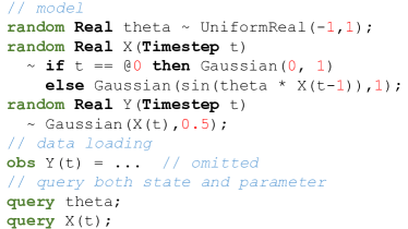
Figure 1: A simple dynamic model in SPEC: the SIN model considered in section 4.1. theta is the parameter. X(t) are latent variables. Y(t) are observed.

3.2.1 Memory Efficient Computation

The particle filtering framework for API is often memory-intensive for applications with a large amount of data. Moreover, inefficient memory management in the inference engine can also result in tremendous overhead at runtime, which in turn hurts the estimation accuracy within a fixed amount of computational budget. Our black-box inference engine also integrates the following compilation optimizations for handling practical problems.

Memory Pre-allocation: Systems that does not manage the memory well will repeatedly allocate memory at run time: for example, dynamically allocating memory for new particles and erase the memory belonging to the old ones after each iteration. This introduces significant overhead since memory allocation is extremely slow. In contrast, SPEC analyzes the input model and allocate the minimum static memory for computation: if the user specifies to run $N$ particles, and the Markov order of the input model is $D$, SPEC will allocate static memory for $(D+1)*N$ particles in the target code. When the a new iteration starts, we utilize a rotational array to re-use the memory of previous particles.

SPEC also avoids dynamic memory allocation as much as possible for intermediate computation step. For example, consider a multinomial distribution. When its parameters change, a straightforward implementation to update the parameters is to re-allocate a chunk of memory storing all the new parameters and pass in to the object of the multinomial distribution. In SPEC, this dynamic memory allocation operation is also avoided by pre-allocating static memory to store the new parameters.

Efficient Resampling: Resampling step is critical for particle filter algorithms since it requires a large number of data copying operations. Since a single particle might occupy a large amount of memory in real applications, directly copying data from the old particles to new ones induce substantial overhead.

In SPEC, every particle access to its data via an indirect pointer. As a result, redundant memory copying operations are avoided by only copying the pointers referring to the actual particle objects during resampling. Note that each particle might need to store multiple pointers when dealing with models with Markov order larger than 1 (i.e., $x_{k}$ depends on both $x_{k-1}$ and $x_{k-2}$, which is supported in SPEC).

SPEC also enhances program locality to speed up resampling. In the compiled code, the indexes of the array which stores the pointers are carefully aligned to take the advantage of memory locality when those pointers are copied.

In our experiment, when dealing with small models where the resampling step takes a large fraction of overall running time, SPEC achieves over 3x to 6x speedup against the fastest benchmark toolkit for PF and PMCMC.

3.2.2 Algorithm Integration:

Currently SPEC supports the bootstrap particle filter, Liu-West filter, PMCMC and API. User can specify any of these algorithms as the inference algorithm as well as the number of particles. The Markov order of the input model will be automatically analyzed.

When choosing API, SPEC analyzes all the static parameters in the model and compiles different approximation distributions for different types of random variables. At the current stage, SPEC supports Gaussian and Mixtures of Gaussian to approximate continuous variables and multinomial distribution for discrete variables. More approximation distributions are under development. For sampling approach, by default SPEC assumes all the parameters are independent and uses deterministic sampling when possible. User could also ask SPEC to generate random samples instead. Furthermore, the number of approximation samples ($M$), the number of mixtures ($L$) can also be specified. By default, $M=7$ and $K=10$.

3.3 Complexity

The time and space complexity of API is $O(NMT)$ over $T$ time steps for generating $N$ particles for $\theta$ and $x$ as well as extra $M$ samples for each particle path to update the sufficient statistics through the moment matching integrals. Setting $N$ and $M$ adequately is crucial for performance. Small $N$ prevents API exploring the state space sufficiently whereas small $M$ leads to inaccurate sufficient statistics updates which will in turn result in inaccurate parameter estimation.

Note that when taking $M$ MCMC iterations, the PMCMC algorithm also has complexity of $O(NMT)$ for $N$ particles over $T$ time steps. However, PMCMC typically requires a large amount of MCMC iterations for mixing properly while very small $M$ is sufficient for API to produce accurate parameter estimation.

Moreover, the actual running time for API is often much smaller than its theoretical upper bound $O(NMT)$. Notice that the approximation computation in API only requires the local data in a single particle and approximation results does not influence the weight of that particle. Hence, one important optimization specialized for API is that SPEC resamples all the particles prior to the approximation step at each iteration and only updates the approximation distribution for those particles that do not disappear after the resampling step. Notice that it is often the case that a small fraction of particles have significantly large weights. Hence in practice, as shown in the experiment section, the overhead due to the $M$ extra samples only causes negligible overhead comparing with the plain particle filter. In contrast, the theoretical time complexity is tight for PMCMC.

4 Experiments

The experiments were run on three benchmark models: 1. SIN: a nonlinear dynamical model with a single continuous parameter; 2. SLAM: a simultaneous localization and Bayesian map learning problem with 20 discrete parameters; 3. BIRD: a 4-parameter model to track migrating birds with real world data. We compare the estimation accuracy of API against Liu-West filter and PMCMC within our compiled inference SPEC. We also compare our SPEC system with other state-of-the-art toolboxes, including Biips and LibBi. Since Biips and LibBi do not support discrete variable or conditional-dependency in the model, we are only able to compare against them on the SIN model.

The experimental machine is a computer equipped with Intel Core i7-3520 and 16G memory.

4.1 Toy nonlinear model

We are considering the following nonlinear model (the modeling code is in Figure 1):

$$x_{t} = \sin(\theta x_{t-1})+v_{t},\quad v_{t}\sim\mathcal{N}(0,1)$$

$$y_{t} = x_{t}+w_{t},\quad w_{t}\sim\mathcal{N}(0,0.5^{2})$$ (11)

where $\theta^{\star}=-0.5$ and $\theta\sim\mathcal{N}(0,1)$ and $x_{0}\sim\mathcal{N}(0,1)$. We generate $5000$ data points using $\theta^{\star}$ from this model. Notice that it is not possible to use Storvik filter (Storvik, 2002) or the particle learning (Lopes et al., 2010) algorithm for this model as sufficient statistics do not exist for $\theta$.

We evaluate the mean square error of the estimation results over 10 trials within a fixed amount of computation time given our generated data points for Liu-West filter, PMCMC and API. Note that all these algorithms are producing samples while ground truth is a point estimate. We take the mean of the samples for $\theta$ produced by Liu-West and API at the last time step. For PMCMC with $M$-MCMC iterations, we take the mean of the last $M/2$ samples and leave the first half as burn-in.

We choose the default setting for API: Gaussian approximation with $M$ samples. For PMCMC, we experiment on different number of particles (denoted by $N$). For proposal of $\theta$, we use a local proposal of truncated Gaussian distribution. We also perform a grid search over the variance of the proposal and only report the best one.

In order to investigate the efficiency of SPEC, we also compare the running time of PMCMC implementation of SPEC against Biips and LibBi. The results are shown in Figure 2.

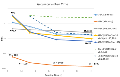
Figure 2: The estimation accuracy of different algorithms with various parameters and implementations on the SIN model. API produces order-of-magnitude more accurate estimation than Liu-West and PMCMC. The PMCMC by SPEC is 6x faster than LibBi.

API produced a result of two orders of magnitude smaller error within the same amount of running time: it quickly produces accurate estimation (error: $1.6*10^{-4}$) using only 1000 particles and 1.5 seconds, which is still 50x smaller than the best PMCMC result after 3 seconds. For PMCMC in LibBi, we utilize $N=30$ particles. Within 3 seconds, it only produces 35 MCMC samples while SPEC finishes 200 iterations. For PMCMC in Biips, just one MCMC step with one particle takes 0.6s, within which SPEC could already produce high quality estimation.

Parallel Particle Filter in LibBi: LibBi supports advanced optimization choices, including vectorization (SSE compiler option), multi-thread (openmp) and GPU (cuda) versions. We experimented on all these advanced versions and chose the fastest one in Figure 2: the single-thread with SSE compiler option. We also experiment on 100, 1000 and 10000 particles on the SIN model in LibBi’s with multi-thread and GPU option. The parallel versions are still slower than the single thread one on 100 and 1000 particles. For 10000 particles, GPU and multi-thread versions are twice faster than the single-thread version. Note that even with 10000 particles, the inference code generated by SPEC is still 20% faster than the parallel versions by LibBi. In practice, parallelization often incurs significant communication and memory overhead, especially on GPU. Also, due to the resampling step, it is non-trivial to come up with an efficient parallel compilation approach for particle filtering. This experiment demonstrates the importance of memory management in practical setting: with memory efficient computations, even a sequential implementation can be much faster than the parallel version.

Bimodal Variant: The above SIN defines a unimodal posterior on the parameter. We are slightly modifying the model as follows in order to explore our algorithm’s performance on multimodal posteriors.

$$x_{t} = \sin(\theta^{2}x_{t-1})+v_{t},v_{t}\sim\mathcal{N}(0,1)$$

$$y_{t} = x_{t}+w_{t},w_{t}\sim\mathcal{N}(0,0.5^{2})$$ (12)

Due to the $\theta^{2}$ term, $p(\theta\mid y_{0:t})$ will be bimodal. We execute API with $10^{3}$ particles and $M=7$ using $K$ mixtures of Gaussian for approximation. We also ran the PMCMC with 100 particles using truncated Gaussian proposal. We ran PMCMC for 10 minutes to ensure mixing. We measure the performance for API with $K=2$, $K=5$ , $K=10$ as well as PMCMC. The histograms of the samples for $\theta$ are illustrated in Figure 3. Comparing with the result by PMCMC, API indeed approximates the posterior well. Note that even with $10^{5}$ particles, Liu-West filter cannot produce a bimodal posterior.

For $K=2$, API was only able to find a single mode. For both $K=5$ and $K=10$, API successfully finds two modes in the posterior distribution, though the weights are more accurate in the case of $K=10$ than $K=5$. This implies that increasing the number of mixtures used for approximation helps improving the probability of finding different modes in the posterior distribution.

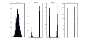
Figure 3: The histograms of the produced samples for $\theta$ in the multimodel example by API with different parameters and by PMCMC. API indeed approximates the true posterior well.

4.2 Simultaneous localization and mapping

We are considering a Simultaneous localization and mapping example (SLAM) modified from (Murphy, 2000). The map is defined as a 1-dimensional grid, where each cell has a static label (parameter to be estimated) which will be observed by the robot. More formally, the map is a vector of discrete random variables $M(i)\in\left\{1,\dots,N_{O}\right\}$, where $1\leq i\leq N_{L}$. Neither the map nor the robot’s location $L_{t}\in\left\{1,\dots,N_{L}\right\}$ is observed. The existing observations are the label of the cell at robot’s current location and the action chosen by the robot.

Given the action (move right ($\rightarrow$) or left ($\leftarrow$)) the robot moves in the direction of action with a probability of $p_{a}$ and stays at its current location with a probability of $1-p_{a}$ (i.e. robot’s wheels slip). The prior for the map is a product of individual cell priors, which are all uniform. The robot observes the label of the cell, it is currently located in correctly, with a probability of $p_{o}$ and incorrectly with a probability of $1-p_{o}$.

In the original example, $N_{L}=8$, $p_{a}=0.8$, $p_{o}=0.9$, and 16 actions were taken. In our experiment, we enhance the model by setting $N_{L}=20$ and duplicating the actions in (Murphy, 2000) several times to finally derive a sequence of 164 actions.

We compare the estimation accuracy over particle filter (PF), PMCMC and API within SPEC. Notice that the Liu-West filter is not applicable in this scenario as artificial dynamics approach can only be performed for continuous parameters. For PMCMC, at each iteration, we only resample a single parameter using an unbiased Bernoulli distribution as the proposal distribution. For API we use $M=50$ approximation samples and a fully factorized (Bernoulli) discrete distribution for approximation.

Since it is still possible to compute the exact posterior distribution, we run these algorithms within various time limits and measure the KL-divergence between the estimated distributions and the exact posterior. The results in Figure  4 show that PF drastically suffers from the sample impoverishment problem; PMCMC fails to get rid of a bad local mode and suffers from poor mixing rates while API successfully approximates the true posterior even with only 1500 particles.

Note that we also measure the running time of API against the plain particle filter on this model. PF uses 0.596s for $3*10^{4}$ particles. For API with $M=50$, although theoretically it would be $N_{L}M=1000$ times slower than PF, it uses only 37.296s for $3*10^{4}$ particles, which is merely 60x slower than PF.

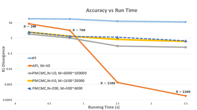
Figure 4: The KL-Divergence between the true posterior and the estimation results produced by different algorithms. PMCMC was trapped in a local model while API quickly produces order-of-magnitude more accurate estimation with only 1500 particles.

Choices of Parameters: We experiment API with different parameters (number of particles $N$ and number of samples $M$) and evaluate the average log KL-divergence over 20 trials. The results in Figure 5 agree with theory. As $N$ increases the KL-divergence constantly decreases whereas after a certain point, not much gain is obtained by increasing $M$. This is due to the fact that for big enough $M$, the moment matching integrals are more or less exactly computed and the error is not due to the Monte Carlo sum but due to the error induced by the ADF projection step. This projection induced error cannot be avoided.

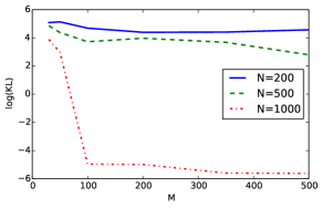
Figure 5: API with various parameters on the SLAM model.

4.3 Tracking bird migration

The bird migration problem (BIRD) is originally investigated in (Elmohamed et al., 2007), which proposes a hidden Markov model to infer bird migration paths from a large database of observations. We apply the particle filtering framework to the bird migration model using the dataset officially released. In the dataset, the eastern continent of U.S.A is partitioned into a 10x10 grid. There are roughly $10^{6}$ birds totally observed in the dataset. For each grid, the total number of birds is observed over 60 days within 3 years. We aim to infer the number of birds migrating at different grid locations between two consecutive days. To sum up, in the BIRD model, there are 4 continuous parameters with 60 dynamic states where each time step contains 100 observed variables and $10^{4}$ hidden variables.

We measure the mean squared estimation error over 10 trials for API with Gaussian approximation ($M=7$), the Liu-West filter and PMCMC with truncated Gaussian proposal distribution within different time limits. The results are shown in the right part of Figure 6 again show that our API achieves much better convergence within a much tighter computational budget.

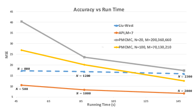
Figure 6: Estimation accuracy of API against Liu-West filter and PMCMC on the BIRD model. API produces significantly better estimation results with smaller amount of computation time.

We again measure the running time of API against the plain particle filter on the BIRD model. PF uses 104.136s while API uses 133.247s for 1000 particles. Note that in this real application, API with $M=7$ only results in 20% overhead compared with PF, although theoretically API should be 28x slower.

5 Discussion

Similar to (Storvik, 2002; Lopes et al., 2010), we are sampling from $p(\theta\mid x_{0:t}^{i},y_{0:t})$ at each time step to fight against sample impoverishment. It has been discussed before that these methods suffer from ancestral path degeneracy (Chopin et al., 2010; Lopes et al., 2010; Poyiadjis et al., 2011). For any number of particles and for a large enough $n$, there exists some $m<n$ such that $p(x_{0:m}\mid y_{0:n})$ is represented by a single unique particle. For dynamic models with long memory, this will lead to a poor approximation of sufficient statistics, which in turn will affect the posterior of the parameters. Poyiadjis et al. (2011) showed that even under favorable mixing assumptions, the variance of an additive path functional computed via a particle approximation grows quadratically with time. To fight against path degeneracy, one may have to resort to fixed-lag smoothing or smoothing. Olsson et al. (2008) used fixed-lag smoothing to control the variance of the estimates. Del Moral et al. (2010) proposed an $O(N^{2})$ per time step forward smoothing algorithm which leads to variances growing linearly with $t$ instead of quadratically. Poyiadjis et al. (2011) similarly proposed an $O(N^{2})$ algorithm that leads to linearly growing variances. Similarly, doing a full kernel move at a rate of $1/t$ on $\left\{x_{0:t},\theta\right\}$ as in (Gilks & Berzuini, 2001) will also be beneficial.

Another important matter to consider is the convergence of the assumed density filtering posterior to the true posterior $p(\theta\mid x_{0:t},y_{0:t})$. Opper & Winther (1998) analyzed the convergence behavior for the Gaussian projection case. There is no analysis of convergence when the moment matching integrals are computed approximately via Monte Carlo sums. However, our experiments indicate that for approximations with sufficiently many Monte Carlo samples, similar convergence behavior as in (Opper & Winther, 1998) is attained. Heess et al. (2013) investigated approximating the moment matching integrals robustly and efficiently in the context of expectation-propagation. They train discriminative models that learn to map EP message inputs to outputs. The idea seems promising and can be applied in our setting as well.

6 Conclusion

In this paper, we present a new inference algorithm, API, for both state and parameter estimation in dynamic probabilistic models. We also developed a black-box inference engine, SPEC, performing API over arbitrary models described in the high-level modeling language of SPEC. SPEC leverages multiple compiler level optimizations for efficient computation and achieves 3x to 6x speedup against existing toolboxes. In our experiment, API produces order-of-magnitude more accurate estimation result compared to PMCMC within a fixed amount of computation time and is able to handle real-world applications efficiently and accurately.

References

- Alspach & Sorenson (1972) Alspach, Daniel L and Sorenson, Harold W. Nonlinear Bayesian estimation using Gaussian sum approximations. Automatic Control, IEEE Transactions on, 17(4):439–448, 1972.
- Andrieu et al. (2010) Andrieu, Christophe, Doucet, Arnaud, and Holenstein, Roman. Particle Markov chain Monte Carlo methods. Journal of the Royal Statistical Society: Series B (Statistical Methodology), 72(3):269–342, 2010.
- Arora et al. (2010) Arora, Nimar S., Russell, Stuart J., Kidwell, Paul, and Sudderth, Erik B. Global seismic monitoring as probabilistic inference. In NIPS, pp. 73–81, 2010.
- Arulampalam et al. (2002) Arulampalam, Sanjeev, Maskell, Simon, Gordon, Neil, and Clapp, Tim. A tutorial on particle filters for on-line non-linear/non-Gaussian Bayesian tracking. IEEE Transactions on Signal Processing, 50(2):174–188, 2002.
- Boyen & Koller (1998) Boyen, Xavier and Koller, Daphne. Tractable inference for complex stochastic processes. In Proceedings of the Fourteenth conference on Uncertainty in artificial intelligence, pp. 33–42. Morgan Kaufmann Publishers Inc., 1998.
- Cappé et al. (2007) Cappé, Olivier, Godsill, Simon J, and Moulines, Eric. An overview of existing methods and recent advances in sequential Monte Carlo. Proceedings of the IEEE, 95(5):899–924, 2007.
- Chopin et al. (2010) Chopin, Nicolas, Iacobucci, Alessandra, Marin, Jean-Michel, Mengersen, Kerrie, Robert, Christian P, Ryder, Robin, and Schäfer, Christian. On particle learning. arXiv preprint arXiv:1006.0554, 2010.
- Del Moral et al. (2010) Del Moral, Pierre, Doucet, Arnaud, and Singh, Sumeetpal. Forward smoothing using sequential Monte Carlo. arXiv preprint arXiv:1012.5390, 2010.
- Elmohamed et al. (2007) Elmohamed, MaS, Kozen, Dexter, and Sheldon, Daniel R. Collective inference on Markov models for modeling bird migration. In Advances in Neural Information Processing Systems, pp. 1321–1328, 2007.
- Erol et al. (2013) Erol, Yusuf B, Li, Lei, Ramsundar, Bharath, and Stuart, Russell. The extended parameter filter. In Proceedings of the 30th International Conference on Machine Learning (ICML-13), pp. 1103–1111, 2013.
- Fearnhead (2002) Fearnhead, Paul. Markov chain Monte Carlo, sufficient statistics, and particle filters. Journal of Computational and Graphical Statistics, 11(4):848–862, 2002.
- Gilks & Berzuini (2001) Gilks, Walter R. and Berzuini, Carlo. Following a moving target – Monte Carlo inference for dynamic bayesian models. Journal of the Royal Statistical Society. Series B (Statistical Methodology), 63(1):127–146, 2001.
- Gordon et al. (1993) Gordon, N. J., Salmond, D. J., and Smith, A. F. M. Novel approach to nonlinear/non-Gaussian Bayesian state estimation. IEE Proceedings F Radar and Signal Processing, 140(2):107–113, 1993. URL http://ieeexplore.ieee.org/stamp/stamp.jsp?arnumber=210672.
- Heess et al. (2013) Heess, Nicolas, Tarlow, Daniel, and Winn, John. Learning to pass expectation propagation messages. In Advances in Neural Information Processing Systems, pp. 3219–3227, 2013.
- Huber & Hanebeck (2008) Huber, Marco F and Hanebeck, Uwe D. Gaussian filter based on deterministic sampling for high quality nonlinear estimation. In Proceedings of the 17th IFAC World Congress (IFAC 2008), volume 17, 2008.
- Julier & Uhlmann (2004) Julier, Simon J. and Uhlmann, Jeffrey K. Unscented filtering and nonlinear estimation. Proceedings of the IEEE, 92(3):401–422, 2004.
- Kantas et al. (2015) Kantas, Nikolas, Doucet, Arnaud, Singh, Sumeetpal S, Maciejowski, Jan, Chopin, Nicolas, et al. On particle methods for parameter estimation in state-space models. Statistical science, 30(3):328–351, 2015.
- Lauritzen (1992) Lauritzen, Steffen L. Propagation of probabilities, means, and variances in mixed graphical association models. Journal of the American Statistical Association, 87(420):1098–1108, 1992.
- Liu & West (2001) Liu, Jane and West, Mike. Combined parameter and state estimation in simulation-based filtering. In Sequential Monte Carlo Methods in Practice. 2001.
- Lopes & Tsay (2011) Lopes, Hedibert F and Tsay, Ruey S. Particle filters and bayesian inference in financial econometrics. Journal of Forecasting, 30(1):168–209, 2011.
- Lopes et al. (2010) Lopes, Hedibert F, Carvalho, Carlos M, Johannes, Michael, and Polson, Nicholas G. Particle learning for sequential Bayesian computation. Bayesian Statistics, 9:175–96, 2010.
- Milch et al. (2005) Milch, Brian, Marthi, Bhaskara, Russell, Stuart, Sontag, David, Ong, Daniel L., and Kolobov, Andrey. Blog: Probabilistic models with unknown objects. In In IJCAI, pp. 1352–1359, 2005.
- Murphy (2000) Murphy, Kevin. Bayesian map learning in dynamic environments. In In Neural Info. Proc. Systems (NIPS, pp. 1015–1021. MIT Press, 2000.
- Murray (2013) Murray, Lawrence M. Bayesian state-space modelling on high-performance hardware using LibBi. arXiv preprint arXiv:1306.3277, 2013.
- Olsson et al. (2008) Olsson, Jimmy, Cappé, Olivier, Douc, Randal, Moulines, Eric, et al. Sequential Monte Carlo smoothing with application to parameter estimation in nonlinear state space models. Bernoulli, 14(1):155–179, 2008.
- Opper & Winther (1998) Opper, Manfred and Winther, Ole. A Bayesian approach to on-line learning. On-line Learning in Neural Networks, ed. D. Saad, pp. 363–378, 1998.
- Poyiadjis et al. (2011) Poyiadjis, George, Doucet, Arnaud, and Singh, Sumeetpal Sindhu. Particle approximations of the score and observed information matrix in state space models with application to parameter estimation. Biometrika, 98(1):pp. 65–80, 2011. ISSN 00063444. URL http://www.jstor.org/stable/29777165.
- Seeger (2005) Seeger, Matthias. Expectation propagation for exponential families. Technical report, 2005.
- Storvik (2002) Storvik, Geir. Particle filters for state-space models with the presence of unknown static parameters. IEEE Transactions on Signal Processing, 50(2):281–289, 2002.
- Todeschini et al. (2014) Todeschini, Adrien, Caron, François, Fuentes, Marc, Legrand, Pierrick, and Del Moral, Pierre. Biips: Software for Bayesian inference with interacting particle systems. arXiv preprint arXiv:1412.3779, 2014.
- Zoeter & Heskes (2005) Zoeter, Onno and Heskes, Tom. Gaussian quadrature based expectation propagation. In Ghahramani, Z. and Cowell, R. (eds.), Proceedings of the Tenth International Workshop on Artificial Intelligence and Statistics, pp. 445–452. Society for Artificial Intelligence and Statistics, 2005.