Galactic Cold Cores VII: Filament Formation and Evolution

Abstract

Context. The association of filaments with protostellar objects has made these structures a priority target in star formation studies. However, little is known about the link between filament properties and their local environment.

Aims. The datasets of the Herschel Galactic Cold Cores Key Programme allow for a statistical study of filaments with a wide range of intrinsic and environmental characteristics. Characterisation of this sample can therefore be used to identify key physical parameters and quantify the role of environment in the formation of supercritical filaments. These results are highly needed in order to constrain theoretical models of filament formation and evolution.

Methods. Filaments were extracted from fields at distance $D<500$ pc with the getfilaments  algorithm and characterised according to their column density profiles and intrinsic properties. Each profile was fitted with a beam-convolved Plummer-like function and quantified based on the relative contributions from the filament ‘core’, represented by a Gaussian, and ‘wing’ component, dominated by the power-law behaviour of the Plummer-like function. These filament parameters were examined for populations associated with different background levels.

Results. Filaments increase their core (M_line,core) and wing (M_line,wing) contributions while increasing their total linear mass density (M_line,tot). Both components appear to be linked to the local environment, with filaments in higher backgrounds having systematically more massive M_line,core and M_line,wing. This dependence on the environment supports an accretion-based model for filament evolution in the local neighbourhood ($D\leq 500$ pc). Structures located in the highest backgrounds develop the highest central $A_{\mathrm{V}}$, M_line,core, and M_line,wing as M_line,tot increases with time, favoured by the local availability of material and the enhanced gravitational potential. Our results indicate that filaments acquiring a significantly massive central region with M_line,core$\geq$M_crit$/2$ may become supercritical and form stars. This translates into a need for filaments to become at least moderately self-gravitating in order to undergo localised star formation or become star-forming filaments.

1 Introduction

The unprecedented resolution and wavelength coverage of the Herschel Space Observatory (Herschel; Pilbratt et al., 2010) has revealed a complex filamentary network present in a wide range of environments and spatial scales. The presence of filaments in the interstellar medium (ISM) and nearby clouds has indeed been investigated for many years with a variety of instruments and techniques (e.g., Bally et al., 1987; Peretto & Fuller, 2009). Herschel Key Programmes such as the Herschel infrared Galactic Plane survey (Hi-Gal; Molinari et al., 2010), the Gould Belt Survey (HGBS; André et al., 2010), and the Herschel imaging survey of OB Young Stellar objects (HOBYS; Motte et al., 2010) have shown their ubiquitous nature in both dense star forming complexes and diffuse, non-star forming fields (e.g., Men’shchikov et al., 2010; Miville-Deschênes et al., 2010).

The above studies have also provided new clues regarding the role of filaments in the onset of star formation for low and high-mass stars (e.g. Arzoumanian et al., 2011; Hill et al., 2012). Latest results point towards a scenario in which prestellar cores form by gravitational fragmentation of unstable filaments (André et al., 2010) with quasi-constant width of $\sim$$0.1$ pc in the solar neighbourhood (Arzoumanian et al., 2011), although with possible variations at farther distances (Schisano et al., 2014). The processes that could give rise to such filaments are varied, ranging from shocks due to insterstellar magnetohydrodynamic (MHD) turbulence (e.g., Padoan et al., 2001) to dynamical events, such as large scale compression (e.g., Peretto et al., 2012). Under the assumption of isothermality and no magnetic field, filament instability can be quantified by the mass per unit length (or linear mass density; here denoted by M_line for consistency with previous studies) greater than a critical equilibirium value (M_crit$=2c_{\mathrm{s}}^{2}/G$; e.g., Inutsuka & Miyama, 1992), a quantity exclusively dependent on temperature through the isothermal sound speed c_s (Ostriker, 1964). The tendency of bound prestellar cores to be associated with those filaments in a supercritical state (M_line$>$M_crit, where M_crit$\sim 16.5$ M_⊙ pc^-1 for a dust temperature of $T\approx 10$ K; e.g., André et al., 2010) make the study of filament properties and evolution crucial for constraining the process of star formation.

The Herschel Galactic Cold Cores Key Programme (GCC; P.I: M. Juvela; Juvela et al., 2012b) observed 116 fields that contained selected clumps from the Cold Clump Catalogue of Planck Objects (C3PO; Planck Collaboration et al., 2011a; Planck Collaboration et al., 2011b). This unbiased sample covers a wide range of environments, Galactic positions, and physical conditions, which makes it ideal for the statistical investigation of properties associated with the compact source population (Montillaud et al., 2015; M2015 hereafter), dust properties (e.g., Juvela et al., 2015b; Juvela et al., 2015a) as well as star and structure formation in the most diffuse fields (Rivera-Ingraham et al; in prep.).

In this work we complement the analysis presented in Juvela et al. (2012b) by carrying out an in-depth study of filamentary properties as a function of environment for the Herschel fields of the GCC Programme. The primary goal of this paper is to present the filament sample, the techniques, and the key observational results needed for constraining theoretical models of filament formation and evolution. Application of results to these models is the topic of a companion paper (Rivera-Ingraham et al. 2016; in prep). This combined study is important in order to quantify the physical processes associated with the origin of unstable filaments and the onset of star formation.

In Sect. 2 we briefly describe the datasets used for this analysis. Section 3 introduces the getfilaments algorithm used for filament detection and selection, while the techniques for filament profile analysis are included in Sect. 4. Results are presented in Sect. 5, and key observational constraints on the formation of star-forming supercritical filaments in gravitationally-dominated evolutionary scenarios are described in Sect. 6. We conclude with a summary of our main results in Sect. 7.

2 Maps and Datasets

The Herschel maps are those already introduced in previous GCC studies. A comprehensive description of the method and techniques used for map creation and processing has been included in Juvela et al. (2012b) and M2015).

The SPIRE maps ($250$ $\mu$m, $350$ $\mu$m, and $500$ $\mu$m; Griffin et al., 2010) were reduced with the Herschel Interactive Processing Environment (HIPE) v.10.0, using the official pipeline with the iterative destriper and the extended emission calibration. The PACS $160$ $\mu$m maps (Poglitsch et al., 2010) were created using Scanamorphos (Roussel, 2013) version 20 with the galactic flag for the drift correction. All maps had colour and zero-point corrections applied as described in Juvela et al. (2012b).

Column density and temperature maps at a $40$″ resolution were produced by fitting spectral energy distributions (SEDs) pixel-by-pixel to the three SPIRE datasets, assuming a dust opacity of $0.1$ cm² g^-1 at $1$ THz (Hildebrand, 1983), with a fixed dust emissivity index of $\beta=2$, and a mean atomic weight per molecule of $\mu=2.33$. While our assumed value for $\mu$ is consistent with previous filament papers (e.g., Arzoumanian et al., 2011) we note that this number differs from the actual molecular weight per hydrogen molecule ($\mu=2.8$; e.g., Kauffmann et al., 2008), and which would be more appropriate in the calculation of $N_{\mathrm{H}_{2}}$ maps. This choice does not affect, however, the main results of this work that depend on the relative properties of the filament population.

The catalog production techniques and final sample of compact sources associated with each field have been presented in M2015). The source list was produced with the multi-scale, multi-wavelength source extraction algorithm getsources (Men’shchikov et al., 2010; Men’shchikov et al., 2012), which was ran simultaneously on the colour and offset-corrected PACS and SPIRE brightness maps, and the column density map. The final catalog was corrected for galaxy contamination and all sources classified according to their stellar content and evolutionary state.

3 Filament Catalog: The getfilaments Method for Filament Detection

Detection and characterisation of filamentary structures in our chosen fields was carried out with the getfilaments  algorithm v1.140127 (Men’shchikov, 2013), an integral part of the getsources  package.

3.1 The getfilaments Approach

Filament characterisation is highly complex because they constitute a hierarchical population in the ISM. The multi-scale nature of filaments has already been observed in molecular studies, such as that presented in Hacar et al. (2013). The innovative detection technique of getfilaments addresses this complexity by identifying different types of filaments according to the spatial scales at which they are detected. A detailed description of the source and filament extraction procedure has been published in Men’shchikov et al. (2012) and Men’shchikov (2013).

In essence, the getfilaments algorithm decomposes the original map into a sequence of spatially filtered ‘single-scale’ images, from the smallest to the largest scales. Each decomposed image contains signals from a narrow range of spatial scales around one particular scale, all substantially larger or smaller scales being filtered out. An important property of the decomposition is that the original image can be recovered by summation of all single-scale images. In each single-scale image getfilaments identifies, by means of an iterative thresholding procedure and several morphological factors, all significantly elongated structures above the image $1\sigma$ fluctuations level. In effect, the masking of all pixels below this level separates the filamentary structures from all other non-filamentary components (sources, background), determining the physical properties (e.g., length and width) of each filament in the single-scale image. All filamentary structures above the threshold are preserved in the single-scale images, whereas all contributions of (compact) sources or background fluctuations are removed, as they are (by definition) not significantly elongated. This results in a set of single-scale images containing all the non-negligible filamentary emission at each particular scale, clean of noise/background contribution. The final reconstructed filament intensity map, containing filamentary information at all spatial scales, is produced by accumulating all the individual (clean) single-scale images of filamentary structures free of background and sources. This process of summation of all spatial scales therefore effectively recovers the complete structural properties of each filament (intensity, length, radial extent) in the map.

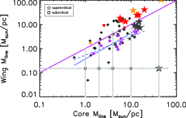
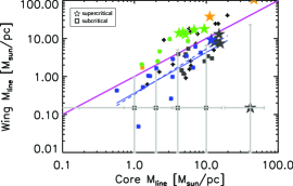
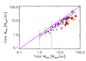
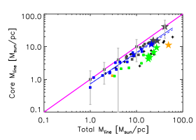
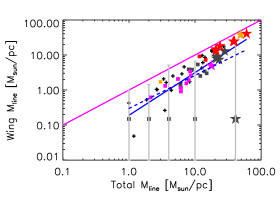
Figure 10: Same as Fig. 8, but with fits performed on the core-dominated sample exclusively.

As the filament extraction algorithm is part of the getsources source extraction method, the code also extracts all sources, separating them from filaments and background. In essence, the getfilaments method carefully separates the structural components (sources, filaments, isotropic background) into different images, which allows one to study the images of the filamentary component fully reconstructed over all spatial scales. Each GCC $N_{\mathrm{H}_{2}}$ map was therefore decomposed into two images: a filament map (free of sources and background contributions), and a source map (free of filament and background). The image of background plus noise was obtained by subtracting both the source and filament images from the original map. For more information and clear illustrations of how the method works, we refer to the intensity profiles in Figs. 2, 15, 17 of Men’shchikov (2013), as well as to the images in Figs. 3–12, 14, 16 in that paper.

By quantifying the filamentary contribution at separate spatial scales, getfilaments permits the analysis of filamentary substructures independently from their larger host filaments. This is critical for a better characterisation of the physics associated with filament formation and evolution, as the properties of filaments associated with a given scale might not necessarily resemble those of filaments reconstructed at substantially larger or smaller scales. Key properties of a particular type of filaments could be missed when investigating just the average characteristics of the entire filament population.

In this work, the extraction and selection of filaments was based on our choice to focus only on those structures most relevant for prestellar core (star) formation (i.e., full-width at half maximum FWHM$<0.2$ pc). Our extraction procedure was therefore tuned to identify structures that have non-negligible filamentary emission at these scales, effectively excluding others that can only be classified as filamentary when including information from larger scales. Examples of the latter could be a filamentary cloud, itself possibly composed of smaller filaments, or other structures only appearing as filamentary-like when including diffuse emission at larger radii. In the multi-scale reality, it is therefore crucial to distinguish and separate these different types of filaments in order to be able to constrain the formation and evolution of a particular subtype. Here we are interested in investigating those filaments that represent the final link to prestellar core formation, or ‘core-scale’ filaments. Filaments significant only when considering larger scales (filaments hosting smaller filaments), being a different type of structure, were excluded from our sample.

In the absence of molecular data capable of confirming structural self-consistency based on velocity information, in the following analysis we define as ‘filaments’ those detections that fulfil the following criteria:

1. significant elongation in the $N_{\mathrm{H}_{2}}$ maps: above the typical elongation in the compact source catalog of $\sim 1.5$;

2. the potential for ‘core-bearing’, i.e., comprising the last step in the hierarchical ladder of the filament population, within the resolution of the data, linked directly to compact source formation;

3. well-behaved and self-consistent entities across the observed spatial scales relevant for star-formation (i.e. physical prestellar core sizes - FWHM${}_{\mathrm{core}}<0.2$ pc) at the resolution of the data.

These criteria reduced the number of available fields for the final analysis, due to the need to exclude distances at which our target filaments would not be resolved. The distribution of distances of the GCC fields range from $D\sim 100$ pc to a few kpc (M2015), which at the resolution of the $N_{\mathrm{H}_{2}}$ maps implies that only those with distance less than $\sim 500$ pc are suitable for the detection of core-bearing filaments with widths comparable to those reported in previous studies ($40$″$\sim 0.1$ pc at $D\sim 500$ pc). In this work we do not consider any field with an estimated distance above this value.

The process for selecting the target core-scale filaments is summarised in the following paragraphs, but we refer to Men’shchikov (2013) for a more detailed description of the algorithm, its data products, and techniques employed.

3.2 Preliminary Detection of Filamentary Structures

The filament identification process is based on the decomposition of the filament emission according to its contribution to separate finely-spaced observed spatial scales ($\theta$). Image decomposition, and ultimately, filament reconstruction, is carried in image units (arcseconds), therefore allowing for the possibility of a given field containing structures (clumps, filaments…) at different distances along the line of sight.

getfilaments produces initially for each field a ‘skeleton’ map for filaments reconstructed in pre-defined ranges of spatial scales $\theta/2$ to $\theta$, where $\theta$ is a multiple of the map resolution ($40$, $80$, $160$, $320$, $640$, and $1280$″). Each $\theta/2$ – $\theta$ skeleton image contains 1-pixel lines tracing the length of filaments along their central part of highest column density (filament ‘crest’ or ‘ridge’). However, each of these images comprises only the filamentary structures detected in the finely-spaced single-scale images in that $\theta/2$ – $\theta$ range. For instance, skeletons in a $40-80$″ scale image mark the position of the ridges of filamentary structures based exclusively on the emission detected in any of the various single spatial scales in that particular spatial scale range, independently of filament properties in spatial scales outside this range. Filaments could be detected in just a few or various single scales (N_scales) within a $\theta/2$ – $\theta$ range. The set of maps ( $\theta=40-80$, $\theta=80-160$″…) therefore progressively remove small spatial scales from the filaments, leaving wider, smoother, and more diffuse filaments. In consequence, skeletons derived from relatively large scales tend to lose precision in tracing the small-scale filament crests in favour of smoother underlying structures. This is advantageous in the large-scale analysis of filaments and ridges with considerable filamentary substructure (e.g., if interested only in the general, averaged properties of the filament group, or filament ‘bundle’; Hacar et al., 2013).

Skeletons based on filaments reconstructed at small scales will, in general, trace the highest column density filaments better than those based on (smoother) filaments reconstructed just from larger scales. The exclusive usage of small scales for filament detection, however, might also result in too conservative ridge tracing. A filament crest does not have to be continuous in nature but may contain regions of enhanced column density. Parts of the same filament that are less centrally condensed and smoother in nature will therefore be removed by the scale filtering, resulting in excessive sub-fragmentation of an otherwise single, long filament. Filaments detected at the smallest scales can therefore be real sub-filaments without a larger scale component (i.e., present only at small scales, or ‘filaments within filaments’), or segments of a longer filament with inhomogeneities along its length in the column density maps.

In this study we restricted the range of spatial scales used for skeleton detection in order to create maps that best reproduced the most prominent filamentary structure as observed in the $N_{\mathrm{H}_{2}}$ maps. This would be in agreement with the filament detection techniques used in other Herschel  studies (e.g., Arzoumanian et al., 2011). However, extra steps had to be taken in order to extract only those structures relevant for prestellar core formation, with non-negligible filamentary emission at the target spatial scales: physical (intrinsic) spatial scales of $\theta_{\mathrm{int}}<0.2$ pc at the distance of the field.

3.3 Filament Extraction

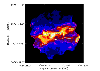
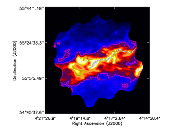
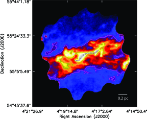
Figure 1: Column density images of the GCC field G149.67+3.56 with reliable filament skeletons superimposed. Detections are those satisfying the minimum selection and detection criteria (see text) when accumulated up to $320$″ for a reliability level N_scales$=10$ (a), N_scales$=30$ (b), and N_scales$=50$ (c). The longest central filament in the field is an example of a well-behaved filament throughout the relevant spatial scales. The $A_{\mathrm{V}}$$=3$ mag (magenta) contours are shown as reference.

Based on our filament definition and selection criteria, the field distance range ($D\sim 100$ – $500$ pc), the compact source size ($0.2$ pc), the spatial scale steps examined by default by getfilaments, and the $40$″  resolution of the $N_{\mathrm{H}_{2}}$ maps, the target core-scale filaments would be detected by examination of spatial scales up to $\theta=80$″ – $320$″($\sim 0.2$ pc at the maximum and minimum distance limits, respectively). While the range of resolved filament physical sizes associated with a given spatial scale varies from field to field according to distance, extraction of all filaments with significant emission from any spatial scales at or below $\theta=320\arcsec$ guarantees that our final sample will contain the type of filaments that are the focus of this work.

To facilitate the identification and extraction of our target filaments, we first created a new single skeleton map that included all filamentary detections up to $\theta_{\mathrm{max}}=320$″. The skeletons of filaments detected in particular scale ranges ($\theta/2$ to $\theta$) were initially provided by getfilaments, but now these needed to be combined in order to produce one single accumulated skeleton map. As mentioned above, a skeleton image associated with the spatial scale range $\theta/2$ – $\theta$ traces the crests of the filaments detected in the various single-scale images in that range. In this map, a skeleton pixel can therefore be quantified based on the number of single scales (N_scales between $\theta/2$ to $\theta$) the skeleton appears in. For practical purposes, the quantity N_scales becomes a measure of reliability: the higher the number of single scales in which the skeleton pixel appears, the higher the reliability of the skeleton. While this does not necessarily imply that skeletons with few N_scales are fake detections, if a filament is self-consistently identified in various scales it is more likely to be a robust filamentary structure, compared to another that looks like a filament only at one single spatial scale. In this case, its classification as filamentary in a particular scale could have been simply fortuitous if it no longer resembles a filament when its emission is examined at smaller or larger scales. Structures that appear as filamentary in just one or two scales are numerous, but this number decreases progressively as we increase the minimum N_scales. This behaviour can be observed in Fig. 1, which illustrates the differences in filament detection arising from application of different reliability (N_scales) limits. This is in fact the same effect observed when decreasing the signal-to-noise (S/N) detection limit when building a compact source catalog. Lowering the S/N (reliability threshold) increases the number of sources in the final list, but it also increases the chances of including spurious detections in the final sample. Skeleton maps produced for each $\theta/2$ to $\theta$ scale range can therefore be associated with a reliability (significance) map, with pixel values representing the number of spatial scales, or N_scales, at which the pixel traces the ridge of a filament in this scale range.

To create an accumulated skeleton map at $\theta\sim 320$″  the significance maps at the spatial scale ranges of $\theta=20-40$″, $\theta=40-80$″, $\theta=80-160$″, and $\theta=160-320$″) were added to obtain a total significance image for the total $\theta=20-320$″ range. In this map, the maximum number of scales associated with any given filament skeleton pixel then depends on its structural prominence along the entire $\theta=20-320$″ range. In other words, each pixel in the significance maps represents the total number of spatial scales in the $\theta=20-320$″ range in which the pixel has been identified as a skeleton pixel of a filament. In this work, the maximum N_scales  (maximum reliability level) of any filament pixel in the accumulated $320$″ significance map was found to be N_scales$\sim 100$. New skeletons could then be derived from this accumulated significance map by thresholding at a chosen minimum N_scales reliability level.

3.4 Filament Selection

Application of a relatively low N_scales reliability level for thresholding the accumulated significance map allows for the detection of filamentary structures dominated by any scales up to $320$″. Depending on the distance, filaments only detected at small scales could be a particular type of filamentary substructure close to the resolution of the data without an external filamentary background. In the opposite extreme, detections would comprise diffuse filaments without prominent substructure, and that appear as ‘filaments’ only when accounting for larger scales approaching $\theta\sim 320\arcsec$.

According to the third criterion of our established filament definition, the goal of this work is to select those detections with ‘well-behaved’ filamentary properties throughout the range of chosen (prestellar core-relevant) spatial scales. A high N_scales reliability level not only increases the robustness of the detection, but it also selects filaments that are more self-consistent throughout the entire range of scales. This results from the limited number of spatial scales detected in any given $\theta/2$ to $\theta$ scale-range provided by getfilaments  and therefore the need of having contributions at more than one spatial scale range in order for the accumulated N_scales to reach the chosen higher minimum reliability level.

We tested the robustness of our results by repeating our analysis using skeleton maps tracing filaments with minimum N_scales reliability levels at regular intervals of N_scales$=10$, $30$, $50$, and $70$. The default level used in our analysis was chosen as N_scales$=10$, which provided a filament sample that overlapped at the $\sim 80$% level with the structures traced by the filament detection algorithm from Schisano et al. (2014). We used the other reliability levels to test the robustness of the results derived with the N_scales$=10$ sample.

In addition to spatial self-consistency, we applied additional reliability criteria to the final skeletons to account for detection (sensitivity) limitations and our previously defined filamentary properties. Pixels associated with filament skeletons required a S/N$>5$ on the original column density map with respect to their associated (column density) uncertainty. These pixels were also required to be above local background level by at least a factor of 1.2 for a filament to be classified as a prominent enough structure with respect to its environment. However, we imposed no limit on the minimum column density associated with background or filament in order to be able to account for the most diffuse fields in our sample (Table 1).

Remaining reliable filamentary ‘segments’ and pixels were removed by excluding all skeletons with length less than $4$ pixels ($\sim 40$″). The final skeleton maps were visually inspected to ensure that they reproduced all major filamentary structures in any given field with the greatest fidelity.

The complexity of the filamentary nature of the ISM and the flexibility of the getfilaments algorithm clearly allows for fine-tuning and variations of our chosen extraction technique. However, our approach that a filament should be classified as ‘significant’ in the chosen accumulated spatial scale not only ensures the identification of reliable filaments relevant for the key star formation scales, but also minimizes the filament sub-fragmentation effect while keeping ‘real’ filamentary substructure. Should contribution from scales larger than $320$″ be necessary in order to make a filament ‘significant’ (N_scales above minimum), such detection would not be considered reliable to enter our classification, even if contributions are nevertheless present at smaller scales. While our filament sample might therefore not be necessarily complete, it contains the most robust and reliable detections of prestellar core-relevant filaments representative of the fields of the GCC Programme.

Here we note that our filament selection technique would not result in biased results regarding filament properties such as width. The core-scale filament selection criterium ($\theta\la 320$″) was used for detection purposes only, i.e., keeping those filaments that are significant detections (i.e., satisfying the N_scales requirement) at core-scales. While this excludes filaments prominent only at larger scales, this does not preclude our final filament sample from having contributions at larger radii (larger widths). Filament characterisation and profile analysis was performed on the image of fully-reconstructed filaments at all scales (separated from the background), therefore taking into account all possible contributions from all available scales in any given field (Men’shchikov, 2013).

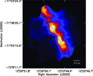
Figure 2: Column density map of the GCC field G300.86-9.00 with the skeleton of the main filament superimposed. Skeleton was obtained with the getfilaments algorithm and N_scales$=10$. The $A_{\mathrm{V}}$$=1$ mag (black) and $A_{\mathrm{V}}$$=3$ mag (magenta) contours are shown as reference.

4 Analysis: Filament Profiling and Characterisation

Analysis of filament properties was carried out on the sample satisfying all the reliability requirements at the crucial star forming scales. Fig. 2 shows an example for the GCC field G$300.86-9.00$ with a minimum reliability level of N_scales$=10$. Filaments in other fields with this reliability level and satisfying all our reliability criteria are shown in Appendix B.

Radial column density profiles were obtained along directions perpendicular to each pixel of the filament skeleton (crest) using the fmeasure utility (part of getfilaments). For profile derivation, we used two sets of background-free column density maps (see Section 3): the filament-only $N_{\mathrm{H}_{2}}$ map, and the filament$+$compact source $N_{\mathrm{H}_{2}}$ map, obtained by adding the filament-only and source-only maps provided by getsources/getfilaments. We produced two different filament catalogs from these sets of images, defined as the ‘source-subtracted’ (SS) and ‘source-included’ (SI) samples, respectively.

Profiles were averaged along the length of the filament to derive mean radial profiles, for the entire filament and separately for both of its sides. An example of such a profile is shown in Fig. 3. For consistency with previous studies, each averaged profile was fitted with an idealized model of a Plummer-like (Whitworth & Ward-Thompson, 2001; Nutter et al., 2008) cylindrical filament (convolved with a $40$″ beam) of the form

$$\rho_{p}(r)=\frac{\rho_{\mathrm{c}}}{[1+(r/R_{\mathrm{flat}})^{2}]^{p/2}}.$$ (1)

Here, $\rho_{\mathrm{c}}$ is the central density, $R_{\mathrm{flat}}$ is the size of the inner flat portion of the filament profile, and p is the exponent (p$\sim 2$) that characterises the power-law behaviour of the profile at larger radii. The inclination angle of the filament relative to the plane of the sky was assumed to be equal to zero. The fitting process was carried out using a non-linear least squares minimization IDL routine based on mpfit (Markwardt, 2009) tracing the entire profile as measured from the background-free $N_{\mathrm{H}_{2}}$ map or to the point of overlap with another filamentary structure. Only those profiles with data extending past the half-maximum width of the filament were used in our analysis. This ensured that the overall shape of the profile and the parameter estimates obtained from the fit were reliably constrained.

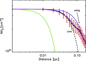
Figure 3: a) Skeleton-averaged filament column density profile (black curve) with best-fit (magenta) Plummer-like function. The best-fit (blue) Gaussian function to the data (no fitting radius restriction) is shown relative to the final best Gaussian function representing the innermost regions of the profile (black dashed-curve) and the $40$″ telescope beam (green). Error bars show the dispersion of column density along the filament. The Gaussian-like inner regions of the profile (core component) can be separated from the wing component of the filament, associated with the (outer) power-law regions of the Plummer profile not accounted for by the Gaussian function. b) Sample of 20 best-fit Plummer-like models (normalised: $N_{\mathrm{H}_{2}}$$=1$ at radial distance from filament centre $R\approx 0$) with varying proportions of core and wing components.

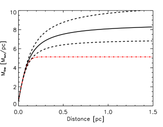
Figure 4: Total linear mass density (M_line,tot) as a function of radial distance from the filament crest for a Plummer-like function (solid black curve) with $R_{\mathrm{flat}}=0.10\pm 0.01$ and $p=2.9\pm 0.2$, relative to a Gaussian with FWHM$=0.18\pm 0.02$ pc (dot-dashed red curve). Changes in the M_line,tot$-R$ relation depend on the uncertainties in the Plummer parameters $R_{\mathrm{flat}}$ and $p$ (black dashed-lines). The Gaussian FWHM was defined as the point where an increase in Gaussian width overestimates the linear mass density of the inner parts of the Plummer function.

The combination of a flat and a power-law component of a Plummer-like function can generally reproduce the observed profile accurately (Fig. 3). However, issues such as the correlation of $R_{\mathrm{flat}}$ and the p-exponent, or the presence of profiles already accurately fitted by a simple Gaussian, can make the true physical meaning of the best-fit Plummer parameters, and their usability toward filament characterisation, questionable (see e.g., Juvela et al., 2012a; Malinen et al., 2012; Smith et al., 2014). Rather than using the absolute values of $R_{\mathrm{flat}}$ and the p-exponent, here we characterise the filament in terms of two alternative morphological descriptors: a core component and a wing component. Identification and separation of each of these two quantities relies in one main assumption, used already in previous studies such as that of Arzoumanian et al. (2011), which claims that the innermost central regions of the filament profile can be represented by a Gaussian function. This Gaussian-like inner component of the profile, which in this work we define as the filament ‘core’ component, can then be quantified separately from the ‘wing’ component, associated with the power-law behaviour of the filament profile and which causes it to deviate from a Gaussian-like shape at larger radii (Fig. 3). The variety of filament core-wing combinations can be observed in the sample of 20 filament Plummer-like profiles included in Fig. 3.

The Plummer parameters ($\rho_{\mathrm{c}}$, $R_{\mathrm{flat}}$, and p-exponent) are only used in deriving the model that fits the filament column density profile best. Such a model replaces the observational data when calculating the relative contributions of the core and wing filament components to the profile. The total linear mass density, M_line,tot, can be calculated by integration of the model Plummer profile:

$$\textit{M}_{\mathrm{line,tot}}=\int\Sigma_{\mathrm{model}}(r)dr=\textit{M}_{\mathrm{line,core}}+\textit{M}_{\mathrm{line,wing}},$$ (2)

with M_line,wing$=0$ for a purely Gaussian profile. Here, M_line,tot remains accurately determined regardless of the final value of the best-fit Plummer parameters, as long as the shape of the profile is well described by such parameters. Overall, integration of the background-free profiles beyond $\sim 1.5$ pc introduces variations in M_line,tot already within $1\sigma$ uncertainty of the linear mass density estimate.

Table 1: GCC fields with filaments at $D\leq 500$ pc^∗ and filaments in SI-sample and N_scales$=10$

Name	l	b	$<$BKG $N_{\mathrm{H}_{2}}$$>^{a}$	$<$Filament $N_{\mathrm{H}_{2}}$$>^{b}$
	[∘]	[∘]	[$10^{20}$ cm-2]	[$10^{20}$ cm-2]
G$0.02+18.02$	$0.03$	$18.03$	$9.5$	$1.1$
G$3.08+9.38$	$2.90$	$9.34$	$11.6$	$3.7$
G$25.86+6.22$	$25.86$	$6.22$	$29.7$	$3.5$
G$116.08-2.40$	$116.13$	$-2.45$	$20.3$	$2.1$
G$126.63+24.55$	$126.65$	$24.55$	$3.3$	$0.4$
G$150.47+3.93$	$150.36$	$3.95$	$29.6$	$9.8$
G$159.23-34.51$	$159.22$	$-34.24$	$8.8$	$3.7$
G$173.43-5.44$	$173.53$	$-5.27$	$10.9$	$0.8$
G$206.33-25.94$	$206.35$	$-26.08$	$2.7$	$2.2$
G$210.90-36.55$	$210.89$	$-36.55$	$7.0$	$2.0$
G$300.61-3.13$	$300.63$	$-3.02$	$17.0$	$1.3$
G$300.86-9.00$	$300.87$	$-9.00$	$11.87$	$5.8$
G$315.88-21.44$	$315.87$	$-21.45$	$3.4$	$1.4$
G$358.96+36.75$	$358.96$	$36.75$	$6.3$	$2.4$
∗ From M2015.
a Average $N_{\mathrm{H}_{2}}$ of background.
b Average $N_{\mathrm{H}_{2}}$ of filament$+$compact source (background-free).

Table 2: Parameter distributions for filament samples with reliability level N_scales$=10$

Sample	Num. Detections	$<$Mline,core$>$	$<$Mline,wing$>$	$<$$N_{\mathrm{H}_{2}}$$>^{a}$	$<$BKG $N_{\mathrm{H}_{2}}$$>$	FWHM
		[M⊙ pc-1]	[M⊙ pc-1]	[$10^{20}$ cm-2]	[$10^{20}$ cm-2]	[pc]
SI	$42$	$5.52\pm 0.63$	$7.36\pm 1.32$	$21.48\pm 2.90$	$21.11\pm 1.79$	$0.13\pm 0.01$
SI${}_{\mathrm{sb}}^{b}$	$29$	$3.79\pm 0.41$	$2.89\pm 0.51$	$13.93\pm 1.60$	$18.57\pm 2.07$	$0.13\pm 0.01$
SI${}_{\mathrm{sp}}^{c}$	$13$	$9.37\pm 1.31$	$17.34\pm 2.44$	$38.31\pm 6.72$	$26.79\pm 3.01$	$0.13\pm 0.02$
SS	$29$	$4.90\pm 0.69$	$5.73\pm 1.90$	$11.37\pm 1.58$	$20.64\pm 2.71$	$0.20\pm 0.01$
SIS	$17$	$5.79\pm 1.21$	$5.51\pm 2.31$	$19.95\pm 4.12$	$20.15\pm 2.74$	$0.13\pm 0.01$
a Average intrinsic (background-removed) $N_{\mathrm{H}_{2}}$ and standard error on the mean of crest.
b Subcritical filaments: Mline,tot$<$Mcrit$\sim 16.5$ M⊙ pc-1.
c Supercritical filaments: Mline,tot$\geq$Mcrit$\sim 16.5$ M⊙ pc-1.

Quantification of the filament characteristic width (and therefore, the Gaussian core-component) based on a best-fit $\chi^{2}$ Gaussian fit to the entire profile becomes, however, problematic for those cases dominated at larger radii by the power-law component of the Plummer-like function. Such a wing component will result in a poor (Gaussian) fit of the central (filament core) region (e.g., Fig. 3) that we wish to separate from the wing component.

To overcome this problem, other studies excluded the wing component by limiting the maximum radius used for the fit (e.g., fitting radius from centre of filament $R<0.5$ pc; D. Arzoumanian; priv. comm.). However, the variety of radii at which the background level is reached does not allow a common fitting radius to be defined that would work for all filaments in the GCC sample. Furthermore, such an approach could easily introduce bias in the estimated widths depending on the range chosen for the fitting process (e.g., Smith et al., 2014). Instead of choosing arbitrary radii to constrain a Gaussian fit, we quantified the width of the filament Gaussian core component by examining M_line,tot as a function of the distance from the centre of the fitted Plummer profile, comparing that to the value predicted for a Gaussian. Fig. 4 shows an example of the increase in M_line,tot with radius for a Plummer-like profile with $R_{\mathrm{flat}}=0.10\pm 0.01$ and $p=2.9\pm 0.2$, relative to that of a Gaussian, with FWHM$=0.18\pm 0.02$ pc. This value defines the width of the core component. It is derived directly from the best-fit Plummer profile of the filament, and is defined as the maximum (deconvolved) FWHM that a Gaussian can have without overestimating the linear mass density of the derived Plummer profile. For larger FWHMs, it can be observed that the Gaussian M_line,tot-R distribution would overestimate that of the Plummer profile. This occurs at the point where the power-law behaviour starts to dominate the shape of the Plummer distribution, at the outer parts of the filament profile.

The linear mass density of the core component, M_line,core, was assumed to be equal to the integrated area of a Gaussian with the defined FWHM. The wing component thus stands for the material not accounted for by the Gaussian, i.e., M_line,wing$=$M_line,tot$-$M_line,core. Uncertainties on these quantities were derived by performing a similar analysis on Plummer profiles varying according to the uncertainties on the default best-fit parameters $R_{\mathrm{flat}}$ and p-exponent, and which alter the dependence of M_line,tot with distance from the filament crest (Fig. 4).

When our new approach for deriving the typical filament width (Gaussian FWHM) was applied to the Plummer parameters from Arzoumanian et al. (2011), the widths we obtained for their filaments were found to be in good agreement (overall well within their estimated $3\sigma$ errors) with those derived by these authors by performing a Gaussian fitting to their Plummer profiles for $R<0.5$ pc.

In addition to profile fitting and linear mass density determination, each filament was characterised based on other intrinsic properties such as length, elongation, average crest column density and temperature, and local background. For the purpose of this analysis, the background level of a filament was assumed to be equal to the average value at the base of the filament crest. This quantity was obtained using the $N_{\mathrm{H}_{2}}$ background images provided by getsources as secondary products for each GCC map (see Section 3). The background estimate was then calculated by averaging the values assigned in this map to the pixels coincident with the filament skeleton. While the background component can include material in the line of sight, the location and proximity of the fields make this possible contribution a minor effect.

Additional filament parameters provided by fmeasure include an estimate of the mean curvature of the filament, as well as the width at half maximum of each averaged profile (not to be confused with the Gaussian FWHM). The averaged column density profiles were corrected when necessary for filament overlap or punctual substructure by averaging only those pixels unaffected by these effects.

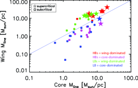
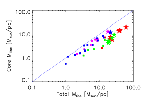
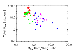
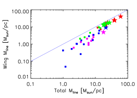
Figure 5: Distributions and correlations of key filament parameters for core-scale subcritical (squares) and supercritical (stars) filaments. Intrinsic total linear mass density M_line,tot, core linear mass density M_line,core, wing linear mass density M_line,wing, and ratio M_line,core$/$M_line,wing. Low-background filaments (LBs: blue/green) are separated from those in denser (high-background) environments with $A_{\mathrm{V}}$$>2.2$ mag (HBs: magenta/red) (see text). For each type of environment, filaments are further separated according to the relative contribution of core/wing components to their M_line,tot: core-dominated (blue/magenta for LBs and HBs, respectively), and wing-dominated (green/red).The 1:1 relation (blue solid line) is shown as reference.

5 Results

Of the 116 regions comprising the field sample of the GCC Programme only 38 have filamentary structure detected by getfilaments. The sample was further reduced with the application of our distance constraint, our filament definition, and the reliability criteria applied to the getfilaments filament catalog. Only those fields at $D\leq 500$ pc (including their $3\sigma$ uncertainty) and with a distance reliability flag$=1$ or $2$ (medium and high level of confidence; M2015) were considered for the analysis. We also excluded filaments that could not be accurately fitted by the Plummer function and those that were visually identified as not being filaments by our chosen definition. Examples of the latter case are those exclusively associated with the elongated head of cometary globules (although we kept those filaments trailing behind such structures).

The final SS-sample comprises 13 fields at D$\leq 500$ pc, with 29 reliable filaments with N_scales$=10$. At the same reliability level, the SI-sample contains a larger number of reliable filaments ($42$ detections in $14$ fields). This is mainly because, without source subtraction, filaments are slightly narrower (satisfying our minimum elongation criterion) and have overall cleaner profiles that extend below half of the maximum value. This final sample remains highly conservative, comprising $\sim 10$% of the original filament population extracted from the GCC fields at N_scales$=10$ and $D\leq 500$ pc, satisfying the distance reliability criteria. The final SI-sample filaments are shown in Appendix B, and the characteristics of their fields are presented in Table 1.

A third filament group was created by selecting those filaments in the SS-sample also classified as reliable in the final SI-sample. This yielded 17 filaments, which we define as the ‘source-included’ subsample, or SIS-sample. Both the SS and SIS samples were only used to quantify the effects of source removal on the parameters derived from the SI-sample, the one chosen as the default filament population for our analysis. Table 2 presents and compares the average filament properties derived for the different samples. The final results, presented in more detail below, are used in the following sections to investigate possible environmental effects on filament formation and evolution.

Figure 5 provides an overview of the distribution of the core-scale filament population separated according to linear mass density and environmental criteria. The plots highlight the relationship between the filament structural components, as well as the relative dominance of each component (core and wing) with respect to M_line,tot. Our final sample comprises filaments with a wide range of intrinsic and environmental properties, as shown in Table 2 and the parameter histograms in Fig. 7. Figure 5 also indicates that the filament sample can be classified into particular sub-populations depending on specific structural properties. Wing-dominated filaments, for instance, are more frequent at high M_line,tot than core-dominated ones, which dominate instead at low M_line,tot. The various filament properties are discussed in more detail in the following sections.

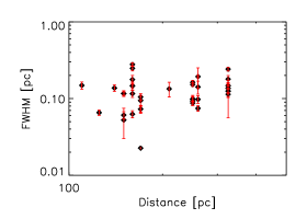
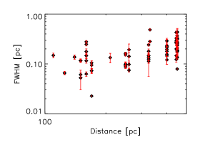
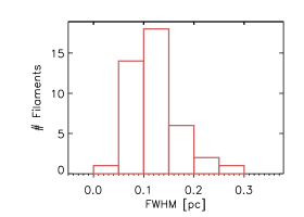
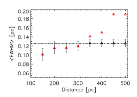
Figure 6: Filament width (Gaussian FWHM) properties for the final SI-sample: (a) filament width as a function of field distance; (b) same as Fig. 6, but without the $3\sigma$ distance uncertainty constraint (see text); (c) width distribution histogram; (d) variation of the (accumulated) average FWHM of filaments with distance for the final sample (triangles with error bars) relative to that of the filament sample in Fig. 6 (red triangles). Dash-dotted line in Fig. 6 marks the median FWHM of the SI-sample.

5.1 Filament Widths

The width distribution and its dependence on distance for the SI-sample are shown in Fig. 6. As seen in Fig. 6 (bin size$=0.05$ pc) the filament population is highly peaked, with a median value of $\approx 0.13$ pc and a standard deviation of $0.05$ pc. These characteristic width and dispersion are somewhat larger than those quoted for filaments in nearby fields of the Gould Belt Survey (e.g., $0.09\pm 0.04$ pc; André et al., 2013), possibly more in tune with predictions from other observational and theoretical studies (e.g., Juvela et al., 2012b; Kirk et al., 2015).

5.1.1 Effects on the Width Distribution

Many factors can affect the observed filament width distribution, from intrinsic differences between populations to more systematic effects, such as distance, filament selection, and source removal.

Distance appears to have a clear influence on the measured width, with the mean FWHM of the population increasing when approaching the telescope resolution limit. This is evident in Figs. 6 and 6 (red curve), which include all the fields with $D\leq 500$ pc in M2015 with filaments detected by getfilaments (without excluding fields not satisfying the criteria of $D\leq 500$ pc when including their $3\sigma$ distance uncertainty. The average width of the population remains close to constant (FWHM$\sim 0.12$ pc) up to $D\sim 300$ pc, after which the mean FWHM increases with distance. The same trend of increasing filament width with distance, albeit less pronounced, is still observed in Fig. 6. This result is likely due to a combination of two main effects.

First, resolution and confusion can decrease the number of detections of $\sim 0.1$ pc-wide filaments at large distances. However, and considering the common hierarchical nature of filaments, unresolved (or barely resolved) filaments could have been detected but only as part of their larger scale (filamentary) host (see e.g., Juvela et al., 2012b; Hacar et al., 2013). In this case, these could appear as resolved filaments, albeit with larger widths, therefore producing the increase in average FWHM with distance. Similarly, small asymmetries in shape and orientation along the filament length (wiggles) might also be undistinguishable at large distances. This effect could result in such filaments appearing more ‘straight’ and with larger average widths, due to the inclusion of the unresolved asymmetries in the overall profile.

Second, our filament detection method was fine-tuned to ensure the extraction of all filaments that are significant detections at the key physical (linear) core-scales. However, the large range of distances considered ($\sim 100-500$ pc) might still have led to the inclusion of some large-scale filamentary structures in our final sample if present in the GCC maps. This is due to the use of a common observed (angular) spatial scale threshold for all fields, which means that (physically) large scale filaments that would be excluded in the nearest fields could have been included in those at larger distances (same angular scale in both cases). Such filaments could then make it to the final sample without being relevant at core-scales if they fulfil the N_scales requirement by using their contributions from larger physical scales. ‘Contamination’ by these structures would affect primarily the fields at the farthest distances (e.g., Fig.6), but could also affect other fields at intermediate distances to a lesser degree.

The magnitude of the effect on the filament width caused by source removal is most likely dependent on the proportion (and location) of the source contribution relative to that of the host filament. Its relevance would also depend on the choice to include or exclude compact sources as part of the filamentary structure and evolution. Based on our findings, however, an influence of the source component on filament modelling could then explain (or significantly contribute to) the presence of a wider width distribution when treating a source-subtracted sample composed of filaments with different degrees of source contribution (e.g., SS vs SIS sample; Table 2).

5.1.2 Identification of Core-scale Filaments

In order to best constrain an evolutionary process leading to star-forming filaments it is crucial to minimize all possible systematic effects. With the effects of resolution and our filament selection method affecting primarily those fields at larger distances, a possible solution would be to reduce the distance range to a maximum of $\sim 300$ pc (e.g., the point of increase in $<$FWHM$>$ in Fig. 6). However, based on telescope resolution, our target filaments could in principle still be detected up to $D\sim 500$ pc. Furthermore, as mentioned above, these effects can also still impact the filament population of nearby fields. Based on this analysis we therefore chose not to reduce the distance upper limit. Instead, we excluded those fields neighbouring the resolution limit of $D\leq 500$ pc in which this effect is expected to be most prominent, and whose distance uncertainty ($3\sigma$) could actually place them beyond this limit. As seen in Fig. 6, this process significantly minimizes the prominent increase in width at large distances observed for the filament sample, resulting in a relatively flat $<$FWHM$>$-$D$ distribution that argues in favour of a characteristic (average) filament width for regions of low-mass star formation in the solar neighbourhood. A similar conclusion was already reached by Arzoumanian et al. (2011) and similar Herschel-based studies (e.g., André et al., 2013).

Application of the $3\sigma$ distance uncertainty requirement shifts the average filament width from $0.19\pm 0.01$ pc to $0.13\pm 0.01$ pc for the final SI sample. However, we note that these values cannot be compared with those found when treating the entire (mixed) filament population. If considering all types of filaments at all scales, and taking into account their well known hierarchical nature, the mean of the entire filament population would most likely shift to a higher value above, therefore more in line with the findings of other studies (e.g., Juvela et al., 2012b; Schisano et al., 2014; Smith et al., 2014).

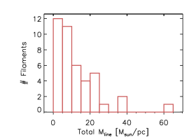
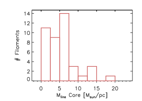
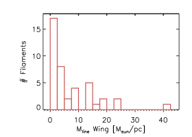
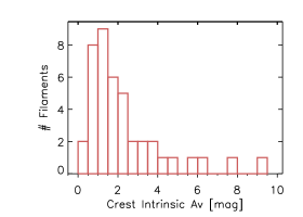
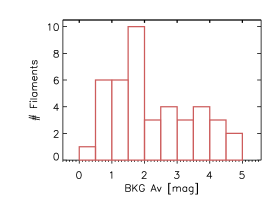
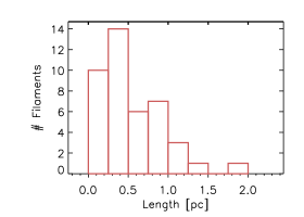
Figure 7: Histograms of key filament parameters for reliable filaments including source contribution (SI-sample): (a) Total linear mass density (M_line,tot); (b) core linear mass density) (M_line,core); (c) wing linear mass density (M_line,wing); (d) crest central $A_{\mathrm{V}}$; (e) background $A_{\mathrm{V}}$; (e) filament length. Blue shading represents the distribution for the core-scale filament sample.

5.2 Filament Length

With a mean length of $\sim 0.5$ pc (Fig. 7: 7), our population clearly differs from the typical pc-scale filaments investigated in other studies (e.g., Hennemann et al., 2012; Palmeirim et al., 2013; Schisano et al., 2014). Such short average length could be associated with real filamentary substructure, but it may not be representative of the overall true mean of the population. The size of the GCC fields (e.g., M2015) already imposed an upper limit on the length of the detections. In addition, the reliability criteria applied in our filament extraction method also frequently resulted in the extraction of just the most reliable ‘segments’ of otherwise longer filamentary structures. The result is a sample more consistent with the sub-pc ‘fibers’ (André et al., 2013) analysed in Hacar et al. (2013), or the ‘branches’ of the main filaments presented in Schisano et al. (2014). As mentioned in the latter study, these shorter structures could be, however, more revealing than the larger ones. The study of more localised regions should be more sensitive to small variations in physical filament properties than results averaged over scales many times above that of a typical prestellar core or clump.

5.3 Stability

Crest $N_{\mathrm{H}_{2}}$ values and total linear mass densities are overall of the same order as those estimated in previous studies (e.g., Arzoumanian et al., 2011; Schisano et al., 2014). Based on total linear mass density criteria, most GCC filaments ($\sim 70$%) are subcritical in nature (M_line,tot$<16.5$ M_⊙ pc^-1), while only one filament would be classified as supercritical based on its M_line,core. Mass estimates from SED fitting are known to underestimate the true mass of high extinction regions in the ISM, including the densest (core) part of the filament profile (see e.g., Pagani et al., 2015 and reliability discussion below). However, the presence of a few young stellar objects (YSOs) could also be explained by localised and sporadic star formation. This could happen in segments of those same filaments but with temperature below and column densities above the mean values, and therefore more favourable for collapse. A more in-depth study of the filament properties of the GCC sample relative to the YSO and compact source population will be presented in a follow-up study.

5.4 Filament Components M_line,core and M_line,wing: Intrinsic Properties

M_line,core and M_line,wing can both vary by several orders of magnitude, with the core and wing components within the ranges of $\approx 0.5-19.5$ M_⊙ pc^-1and $\approx 0-40.5$ $M_{\odot}$ pc^-1, respectively. Overall, M_line,tot varies between $1.0$ and $60$ $M_{\odot}$ pc^-1. Filaments were broadly classified according to the relative contribution of the core and wing components to their M_line,tot. Detections dominated by the core component, M_line,core$>$M_line,wing, were classified as ‘core-dominated’ filaments. Those whose M_line,tot could be accounted for mainly by the contribution from their wing component (M_line,core$<$M_line,wing) were classified as ‘wing-dominated’. This allowed for a direct quantification of the relevance and influence of the core component (the region concentrating the highest column densities and the most relevant for star formation). Here we chose to remain consistent with the standard approach used in Arzoumanian et al. (2011) and later studies, and classified as ‘subcritical’ those filaments with M_line,tot$<$M_crit ($\sim 16.5$ M_⊙ pc^-1 at $T=10$ K), and ‘supercritical’ when M_line,tot$\geq$M_crit. While convenient for the purpose of this work, such terminology is, however, likely incomplete and inappropriate to fully describe the stability state of a filamentary structure (e.g., Fischera & Martin, 2012). Even when using this standard stability description, it is also crucial to distinguish massive filaments with a high M_line,core, with the highest potential for local collapse, from other (low M_line,core) structures that appear supercritical only because of their very extended wing component. A very extended wing (flat profile at large radii) could contribute significantly to the mass but might not be (or lead to) a star-forming filament if associated with a very low M_line,core. This difference is particularly important in the investigation of a possible filament evolutionary scenario.

5.5 Reliability and Robustness of the Results

Filament studies are subject to well-known caveats that should be taken into consideration.

The stability criteria based on filament linear mass density is dependent on observables that are generally difficult to constrain, such as the filament (wing) radius of integration and the background level. Simplifying assumptions, such as one (isothermal) filament temperature or a Gaussian-like morphology for the innermost parts of the filament, might not necessarily be accurate approximations. Similarly, due to the lack of molecular data we cannot confirm that all of our filament detections are also self-consistent (single) structures in velocity as they seem to appear in the Herschel dust maps (and not due to a convenient superposition of structures in the line of sight with the general appearance of a filament). Inclination effects (Arzoumanian et al., 2011), which have not been included in the present analysis, might affect the observed range of linear mass densities, but should not affect conclusions based on the relative behaviour (formation/evolution) of the different filament populations in different environments.

Prominent and dense filaments in star-forming complexes can be, overall, much better constrained, identified, and characterised due to, e.g., a higher $N_{\mathrm{H}_{2}}$ contrast with the environment, or the presence of YSOs tracing the structure itself. For the same reasons, we expect a higher degree of uncertainty in diffuse and non-star forming environments. Here we have aimed to minimize the impact of such detections on our (statistical) conclusions by testing our results on filament populations with increasing reliability (N_scales) level. An increase in N_scales reduces the number of filaments in a sample, but it also increases the robustness of the derived filament properties. In this study, all our results and conclusions hold for samples with different reliability levels and are consistent within $3\sigma$. Source removal has negligible impact on the main results of this work, the major effects being, however, an increase of the average filament width (Table 2) and a systematic decrease of the filament crest column density by a factor of $\sim 2$.

All filaments and measurements are ultimately affected by the assumptions made in the creation of the original column density maps, and from which the filaments are extracted.

First, our neglect of radiative transfer in the derivation of our $N_{\mathrm{H}_{2}}$ and $T$ maps in favour of SED fitting has been known to underestimate the true column density. This is caused by the presence of a dust population consisting of dust grains with a mixture of properties (e.g., Ysard et al., 2012). Indeed, a considerable fraction of cold dust (T$<10$ K) can be missed simply due to warmer dust dominating the modelling of the SED (Pagani et al., 2015). These effects would be predominantly associated with the filament core component, due to it being associated with material with higher extinction. Similarly, the properties of dust grains can also evolve depending on local environmental conditions (e.g., Roy et al., 2013; Ysard et al., 2013). This implies that the use of a constant opacity cannot be appropriate for describing the evolution of a dust-based structure formed by regions (e.g., core, wing components) with different (and varying) physical properties (e.g., an accreting filament growing in mass with time). All these effects are difficult to quantify, and their inclusion in the filament analysis is beyond the scope of this work (albeit consistent with similar previous studies mentioned in this work and that also ignore these effects). These uncertainties are expected to be minimized for our main results, based on the observed relative trends and properties of the population as a whole, but such effects remain crucial for any in-depth model associated with structures in the ISM.

Based on these caveats, the current approach remains simple, especially considering the complexity of filament detection and characterisation (e.g., selection effects, star formation history, and the currently undistinguishable changes in the core and wing contributions for filaments in formation and those already in dispersal stage). Filaments are also subject to many processes (general dynamics, turbulence, magnetic field contributions, etc.), all capable of affecting the observed properties of the filament population. This complexity should always be kept in mind when interpreting the results.

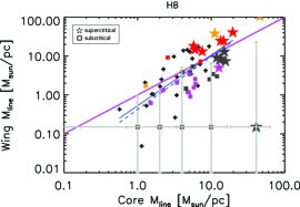
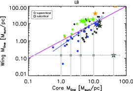
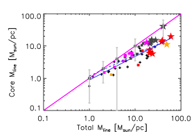
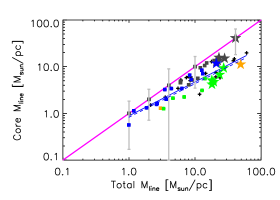
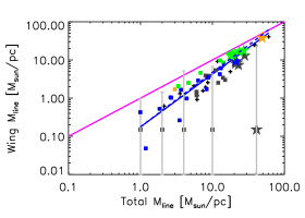
Figure 8: Correlation of M_line,core, M_line,wing, and M_line,tot for core-scale filaments in high backgrounds (filled red and magenta symbols in Figs. 8, 8, 8) and low backgrounds (filled blue and green symbols in Figs. 8, 8, 8). Best linear fits according to environment and for the entire population (background-independent) are shown as (blue) dashed and solid lines, respectively. Plots include the parameters derived for filaments from Arzoumanian et al. (2011): core-dominated (dark grey) and wing-dominated (orange) symbols. Errors bars are shown only for filaments consistent with having no wing contribution (assigned a default value of M_line,wing$=0.1$ $M_{\odot}$ pc^-1 for plotting purposes). Here, uncertainties for the core and wing contributions are those estimated for the core component based on their quoted uncertainties on width and column density. As reference, black crosses in Figs. 8, 8, 8 mark the position of filaments in low-backgrounds. Crosses in Figs. 8, 8, 8 mark those in high-backgrounds. Other symbols, lines, and colours as in Fig. 5.

6 Discussion: Observational Constraints for Filament Models

The GCC filament sample covers structures with a wide range of physical and environmental conditions. We use this sample to identify and constrain particular properties of the filament population that can serve as an observational basis for theoretical models addressing the origin of star-forming filaments.

6.1 Diversity of Filaments: Global Characteristics

Under the standard assumption of star formation in filaments with linear mass density close to M_crit, we can distinguish clear structural properties that filaments must satisfy (e.g., by evolution with increasing M_line) in order to achieve criticality.

Figure 5 reveals distinct types of filaments based on their M_line,core and M_line,wing values. A link between the filament core and wing parameters is evident in Fig. 5, with M_line,wing increasing with M_line,core following a best linear fit ($Y=bX+c$) of $b=1.3\pm 0.2$ and $c=-0.3\pm 0.1$ $M_{\odot}$ pc^-1, as derived from the logarithmic distribution. The trend of increasing M_line,wing with M_line,core therefore conveys a shift from a regime dominated by subcritical filaments to a supercritical one, i.e., an increase of M_line,tot(Figs. 5 and 5).

Filaments in the low end of the M_line,core$-$M_line,wing distribution (Fig. 5), or equivalently, in the M_line,tot$-$M_line,core or M_line,tot$-$M_line,wing diagrams (Figs. 5 and 5) are also characterised by a dominant core component (i.e., ‘core-dominated’ filaments). However, the overall faster increase in M_line,wing than M_line,core with M_line,tot, as shown by the steeper trend for the former ($b_{\mathrm{wing}}=1.38\pm 0.09$, c.f., $b_{\mathrm{core}}=0.73\pm 0.06$), results in a tendency for filaments to lower their M_line,core$/$M_line,wing ratio with increasing M_line,tot, even with the simultaneous increase of both parameters (Fig. 5). The final result is a clear tendency of subcritical filaments to be core-dominated ($\sim 75$% of the subcritical population), while supercritical filaments are predominantly ($\sim 85$%) wing-dominated.

The highlighted behaviour of the derived filamentary properties allows us to define three main ‘Regimes’ in the population. The bulk characteristics of each Regime are summarised in Tables 3 and 4.

• Regime 1: Massive supercritical filaments are predominantly ($\sim 85$%) wing-dominated, with minimum M_line,core and M_line,wing of $\approx 4.2$ $M_{\odot}$ pc^-1 and $\approx 5.0$ $M_{\odot}$ pc^-1, respectively. Filaments with M_line,core$<4.2$ $M_{\odot}$ pc^-1 are therefore exclusively subcritical and predominantly ($70$%) core-dominated.

• Regime 2: The filament population with M_line,core$\geq 4.2$ $M_{\odot}$ pc^-1 contains a mixture of supercritical and subcritical filaments with mixed proportions of core and wing components, environments, and crest column densities. The maximum M_line,core derived for any subcritical filament is found to be M_line,core$\approx 8.4$ $M_{\odot}$ pc^-1, above which only supercritical structures are found. The region in the range $4.2\leq$M_line,core$\leq 8.4$ $M_{\odot}$ pc^-1 therefore defines a ‘transition’ regime, comprised of wing-dominated supercritical ($\sim 34$% of the filaments in this regime) and core and wing-dominated subcritical filaments. A total of $\sim 53$% of all filaments in this Regime are core-dominated filaments.

• Regime 3: A third region, comprised exclusively of supercritical filaments, is also characterised by having the most massive core components and all core-dominated supercritical filaments. This regime contains all filaments with M_line,core$>8.4$ $M_{\odot}$ pc^-1 and with properties consistent with those associated with the actively star-forming supercritical filaments investigated in Arzoumanian et al. (2011). Such centrally massive filaments, associated with the highest column densities, hold the greatest potential for star formation relative to other apparently massive structures with lower M_line,core in Regime 2. As with Regime 2, the sample is comprised of filaments with mixed proportions of M_line,core and M_line,wing components ($\sim 33$% core-dominated).

Table 3: Overview of Average Filament Intrinsic & Environmental Properties in Each Regime.

Regime	BKG Classa	$<$BKG$>^{b}$	$<$BKG$>^{c}$	$<$Ridge $N_{\mathrm{H}_{2}}$$>^{d}$	$<$FWHM$>$
		[$10^{21}$ cm-2]	[mag]	[$10^{21}$ cm-2]	[pc]
1	LB$+$HB	$1.4\pm 0.2$	$1.5\pm 0.2$	$0.9\pm 0.1$	$0.11\pm 0.01$
2	LB$+$HB	$2.6\pm 0.3$	$2.7\pm 0.3$	$2.3\pm 0.3$	$0.14\pm 0.01$
3	LB$+$HB	$2.8\pm 0.4$	$2.9\pm 0.5$	$5.2\pm 0.8$	$0.12\pm 0.01$
a High-background [HB] or low-background [LB].
b Average $N_{\mathrm{H}_{2}}$ of the environment with standard error on the mean.
c $A_{\mathrm{V}}$$=$$N_{\mathrm{H}_{2}}$$/(9.4\times 10^{20})$
d Background-removed.

Table 4: Overview of Average Filament [M_line] Properties in Each Regime.

Regime	Wing/corea	Criticalityb	Mline,core	$<$Mline,core$>$	$<$Mline,wing$>$
			$[M_{\odot}$ pc-1]	[% Mline,tot]	[% Mline,tot]
1	core	SB	$<4.2$	$58$	$42$
2	core$+$wing	SB$+$SP	$4.2\leq M\leq 8.4$	$52$	$48$
3	wing	SP	$>8.4$	$45$	$55$
a Filament type characterising population ($\ga 60$%): wing-dominated [wing]
or core-dominated [core].
b Subcritical [SB] or supercritical [SP] filaments.

These results establish the direction (M_line,core and M_line,wing behaviour with M_line,tot) and final conditions (supercritical filaments in Regime 2 and Regime 3) that must be accounted for by a potential evolutionary process leading to the formation of star-forming filaments. The identification of (structurally) distinct filament regimes could also indicate variations and/or limitations in the formation and evolution process of filaments in gravitationally-dominated scenarios.

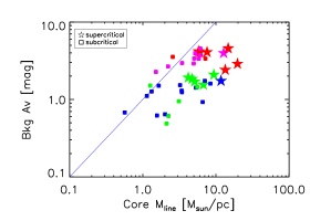
Figure 9: Distribution of filament background level as a function of M_line,core (a) and intrinsic (crest) $A_{\mathrm{V}}$ (b) for the core-scale filament sample. Symbols, lines, and colours as in Fig. 5.

6.2 The Role of Environment In Filamentary Properties and Evolution

In order to constrain the influence of the environment on the properties and/or evolution of the filament core and wing components, filaments were divided into low-background (LB) and high-background (HB) populations. LB filaments were classified as those with average background level below the mean of the population of $N_{\mathrm{H}_{2}}$$\approx 2\times 10^{21}$ cm^-2 ($A_{\mathrm{V}}$$\approx 2.2$ mag), while HB filaments are associated with environmental column density above this value.

The main results of this analysis are summarised in Fig. 8, which investigates the behaviour of the HB and LB populations individually by performing a $\chi^{2}$ fitting to the different parameter distributions of the core-scale filament sample. The figure also shows the core and wing component distributions estimated for the filament sample from Arzoumanian et al. (2011). Here, the core component was derived assuming a Gaussian with the FWHM and central $N_{\mathrm{H}_{2}}$ quoted by these authors in their Table 1. The wing component was calculated by subtracting this core contribution from their derived M_line,tot.

Overall, independent fits to the HB and LB subsamples reveal negligible environmentally-based differences (considering the $1\sigma$ error of the best-fit parameters) for the correlations between M_line,core, M_line,wing, and M_line,tot. With the GCC filaments covering a range of background levels that can differ by a factor of $\sim 10$ ($N_{\mathrm{H}_{2}}$$\sim 0.5-4.5\times 10^{21}$ cm^-2; e.g., Table 2) this is suggestive of a common dominant process (taking place in a wide range of environments, albeit not necessarily at the same magnitude) driving the formation and/or evolution of the majority of our filament population (e.g., turbulence, shocks, or gravity).

Evidence for an environmental dependence of M_line,core might be observed, however, based on its correlation with background level, as shown in Fig. 9. At similar width, M_line,core depends exclusively on the Gaussian peak of the filament profile. This would naturally lead to the correlation in Fig. 9 between background and crest column density. Indeed, the limits of the parameter range for both M_line,core and crest $N_{\mathrm{H}_{2}}$ increase with the $N_{\mathrm{H}_{2}}$ of the environment. The maximum M_line,core (or crest $N_{\mathrm{H}_{2}}$) for HB filaments can double those of the LB sample, with supercritical filaments clustering at the highest backgrounds of $<$$N_{\mathrm{H}_{2}}$$>$$\approx(2.7\pm 0.3)\times 10^{21}$ cm^-2 ($<$$A_{\mathrm{V}}$$>\sim 3$ mag; Fig. 9).

While the shift of the minimum intrinsic (crest) $N_{\mathrm{H}_{2}}$ and M_line,core to higher values with environment could artificially arise from our initial filament detection criteria, these should not have an effect on the upper limits. Indeed, the real origin of our result is further supported by the findings of Schisano et al. (2014), who observed that denser filaments appear to be associated with denser environments. The filament Regimes, separated according to increasing M_line,core and therefore, according to increasing star-forming potential, are also associated with increasingly higher environmental average column density values (Table 3).

Compared to M_line,core, M_line,wing is observed to have a stronger dependence with M_line,tot, regardless of the environment and stability state of the filament (Fig. 5). This leads to the already mentioned tendency of subcritical filaments to be core-dominated. The preference for the most massive wing components to be associated with the most massive M_line,core and M_line,tot (e.g., Figs. 5; 5), can be explained if the wing (power-law) component dominates at a later stage of evolution (under the assumption of M_line,tot increasing with time). Furthermore, the clear tendency of M_line,wing to reach systematically higher values in high backgrounds (Figs. 8, 8) seems to suggest that the formation of the wing component, together with that of supercritical filaments, is intimately linked to processes and conditions primarily associated with such dense environments. A filament evolution and wing origin driven by gravity (accretion, collapse) would be consistent with these results. The availability of mass and the increase in gravitational potential of the filament with time would lead to filament growth and late stages of evolution associated with massive core and wing components.

Overall, we conclude that filament behaviour appears to be dominated by a significant correlation between the various structural components, with the most massive M_line,wing being preferentially associated with the most massive M_line,core and M_line,tot. For similar filament widths, the Gaussian function explains the correlation between M_line,core and crest $A_{\mathrm{V}}$. However, the observed dependence of M_line,core (and crest $A_{\mathrm{V}}$) on the column density of the environment, together with the identification of filament regimes with structural characteristics depending on the background level, strongly suggests that filament formation and evolution is intimately linked to the conditions set by their environment.

7 Conclusions

In this work we have presented an extensive characterisation of the filament population present in the Herschel fields of the Galactic Cold Cores Programme at $D<500$ pc. The sample was used to identify and quantify key observational constraints, in regards to the structure and environment of filaments, needed for the development of theoretical models addressing filament formation and evolution.

Filaments were identified and extracted with the getfilaments algorithm, and classified according to the spatial scales at which they dominate. Filament morphology was characterised by fitting a Plummer-like function to the column density profiles. However, in order to avoid the inherent uncertainties associated with the physical meaning of the Plummer parameters, the structure of the filament was analysed instead with an approach that quantifies the Plummer-like shape according to the relative contribution to the profile (linear mass density) from two components: a central Gaussian-like region, or core component, and a wing component, represented by the power-law tail at larger radii. The filament morphology and intrinsic properties (column density distribution, width, stability) were then examined as a function of local column density background.

(i) We find that the filament characteristic width is highly dependent on distance and compact source association. This value can also be affected by the intrinsically complex hierarchical nature of filaments, which can lead to radically different values depending on the type of filaments being examined. Selection of filaments associated with prestellar core formation, or ‘core-scale’ filaments, reveals a characteristic mean width of $\sim 0.13$ pc for low-mass star forming regions in the local neighbourhood ($D\leq 300$ pc). The combined analysis of all types of filaments and without distance correction would lead to a larger mean for our sample of FWHM$\ga 0.2$ pc.

(ii) The core and wing filament components appear to be environment-dependent, with filaments at higher backgrounds systematically reaching higher core, wing, and total linear mass densities. The association of the most massive wing components with the most massive core components, densest environments, and highest total linear mass densities, support a (late) wing formation driven by accretion and enhanced by the combined effects of large gravitational potential and availability of material. The relative contribution of the core and wing components to M_line,tot varies significantly, but all filaments with a central component M_line,core$\ga 8.5$ $M_{\odot}$ pc^-1 ($\sim$M_crit/2) are supercritical.

(iii) The distribution of linear mass densities of the core (M_line,core) and wing (M_line,wing) components of the core-scale filament sample was used to identify three main filament regimes: a core-dominated subcritical region (Regime 1; M_line,core$<4.2$ $M_{\odot}$ pc^-1), a transition region (Regime 2; $4.2\leq$M_line,core$\leq 8.4$ $M_{\odot}$ pc^-1), and a supercritical-only region (Regime 3; M_line,core$>8.4$ $M_{\odot}$ pc^-1). Each regime is characterised by a progressively higher background column density level, clearly indicating that the environment is key for the development of the filament structure and, ultimately, the formation of supercritical filaments.

Appendix A Filament Analysis: Figures

Appendix B GCC Fields with SI-sample filaments and N_scales$=10$

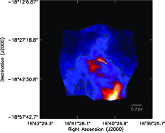
(a) G0.02+18.02

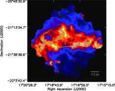
(b) G3.08+9.38

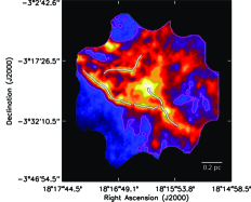
(c) G25.86+6.22

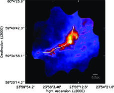
(d) G116.08-2.40

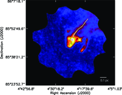
(e) G126.63+24.55

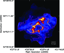
(f) G150.47+3.93

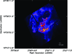
(g) G159.23-34.51

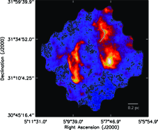
(h) G173.43-5.44

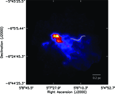
(i) G206.33-25.94

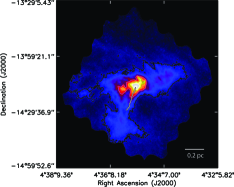
(j) G210.90-36.55-1

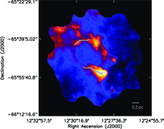
(k) G300.61-3.13

(l) G300.86-9.00

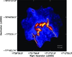
(m) G315.88-21.44

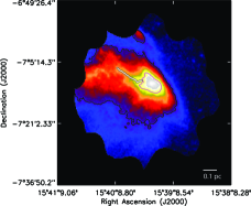
(n) G358.96+36.75

%