Finite element method for nonlinear Riesz space fractional diffusion equations on irregular domains

Abstract

In this paper, we consider two-dimensional Riesz space fractional diffusion equations with nonlinear source term on convex domains. Applying Galerkin finite element method in space and backward difference method in time, we present a fully discrete scheme to solve Riesz space fractional diffusion equations. Our breakthrough is developing an algorithm to form stiffness matrix on unstructured triangular meshes, which can help us to deal with space fractional terms on any convex domain. The stability and convergence of the scheme are also discussed. Numerical examples are given to verify accuracy and stability of our scheme.

1 Introduction

In recent years, fractional calculus is becoming more and more popular among various fields due mainly to its widely applications in science and engineering, see [1, 2, 3, 4, 5]. In physics, space fractional derivatives are used to model anomalous diffusion (super-diffusion and sub-diffusion). In water resources, fractional models are used to describe chemical and pollute transport in heterogeneous aquifers [6].

Owing to fractional differential equations’ various applications, seeking effective methods to solve them is becoming more and more important. There are a large volume of literatures available on this subject. Researchers have presented many analytical techniques for solving fractional differential equations, such as Fourier transform method, Laplace transform method, Mellin transform method, and Green function method [5]. However, it is difficult to find the close forms of most fractional differential equations, and the close forms are always represented by special functions, such as Mittag-Leffler function, which means they are difficult to represent simply and compute directly. Moreover, most nonlinear equations are not solvable by analytical methods, so researchers have to resort to numerical methods.

Over the last few decades, many classical numerical methods have been extended to solve fractional differential equations, such as finite difference method [7, 8, 9, 10], finite element method (FEM) [11, 12, 13, 14], and spectral method [15, 16, 17, 18].

As an efficient method widely used in engineering design and analysis, FEM has been deeply studied by a number of scholars to solve fractional differential equations. Ervin and Roop [13] defined directional integrals and directional derivatives, and developed a theoretical framework for the variational problem of the steady state fractional advection-dispersion equation on bounded domains in $\mathbb{R}^{d}$. Deng [19] investigated FEM for the one-dimensional space and time fractional Fokker-Planck equation. In [20], adopting FEM, Zhang, Liu and Anh solved one-dimensional symmetric space-fractional differential equations. Zhang and Deng [21] proposed FEM for two-dimensional fractional diffusion equations with time fractional derivative. In [22], the authors considered FEM for the space fractional diffusion equation on domains in $\mathbb{R}$. Deng and Hesthaven [23] proposed a local discontinuous Galerkin method for the fractional diffusion equation, and offered stability analysis and error estimates. Wang and Yang [24] derived a Petrov-Galerkin weak formulation to the fractional elliptic differential equation and proved that the bilinear form is weakly coercive. Bu et al. [25, 26, 27] considered two-dimensional space fractional diffusion equations on rectangle domains solved by FEM. In [28], Qiu et al. developed nodal discontinuous Galerkin methods for fractional diffusion equations on 2D irregular domains and provided stability analysis and error estimates. Du and Wang [29] introduced a fast FEM for 2D space-fractional dispersion equations by exploiting the structure of stiffness matrix for rectangular mesh on rectangular domain. As we can see, many works on FEM are limited in solving fractional differential equations with linear source term on rectangle domains with regular meshes. Two-dimensional space fractional problems with nonlinear source term defined on irregular domains, especially partitioned with unstructured meshes, are seldom considered, although they are more real and more useful.

In this paper, we consider the two-dimensional Riesz space fractional diffusion equation on convex domain $\Omega$ with initial condition and boundary condition:

$$\left\{\begin{aligned} &\frac{\partial u}{\partial t}=K_{x}\frac{\partial^{2\alpha}u}{\partial|x|^{2\alpha}}+K_{y}\frac{\partial^{2\beta}u}{\partial|y|^{2\beta}}+F(u)+f(x,y,t),\quad(x,y,t)\in\Omega\times(0,T],\\ &u(x,y,0)=\varphi(x,y),\quad(x,y)\in\Omega,\\ &u(x,y,t)=0,\quad(x,y,t)\in\partial\Omega\times(0,T],\end{aligned}\right.$$ (1)

where $\frac{1}{2}<\alpha,\beta<1$, $K_{x}>0,K_{y}>0$, and $F(u)\in C^{1}(\Theta)$ is a nonlinear function ($\Theta$ is a proper close domain). Boundaries of $\Omega$ are defined as follows (Fig. 1):

Figure 1: Convex domain $\Omega$ with its boundary $a(y),b(y),c(x),d(x)$.

$$\left\{\begin{aligned} a(y)&=\min\{x:(x,\eta)\in\Omega,\eta=y\},\\ b(y)&=\max\{x:(x,\eta)\in\Omega,\eta=y\},\\ c(x)&=\min\{y:(\xi,y)\in\Omega,\xi=x\},\\ d(x)&=\max\{y:(\xi,y)\in\Omega,\xi=x\}.\\ \end{aligned}\right.$$

In Eq. (1), Riesz derivatives [5] $\frac{\partial^{2\alpha}u}{\partial|x|^{2\alpha}}$ and $\frac{\partial^{2\beta}u}{\partial|y|^{2\beta}}$ are defined by

$$\frac{\partial^{2\alpha}u(x,y,t)}{\partial|x|^{2\alpha}} =-c_{\alpha}\left({}_{a(y)}D_{x}^{2\alpha}u(x,y,t)+{}_{x}D_{b(y)}^{2\alpha}u(x,y,t)\right),$$ (2)

$$\frac{\partial^{2\beta}u(x,y,t)}{\partial|y|^{2\beta}} =-c_{\beta}\left({}_{c(x)}D_{y}^{2\beta}u(x,y,t)+{}_{y}D_{d(x)}^{2\beta}u(x,y,t)\right),$$

where $c_{\alpha}=\frac{1}{2\cos(\alpha\pi)}$, $c_{\beta}=\frac{1}{2\cos(\beta\pi)}$, and the operators ${}_{a(y)}D_{x}^{\mu}u(x,y)$, ${}_{x}D_{b(y)}^{\mu}u(x,y)$, ${}_{c(x)}D_{y}^{\mu}u(x,y)$, ${}_{y}D_{d(x)}^{\mu}u(x,y)$ ($n-1<\mu<n,n\in\mathbb{N}$) are defined as [3]

$${}_{a(y)}D_{x}^{\mu}u(x,y,t) =\frac{1}{\Gamma(n-\mu)}\frac{\partial^{n}}{\partial x^{n}}\int_{a(y)}^{x}{(x-s)}^{n-\mu-1}u(s,y,t)ds,$$

$${}_{x}D_{b(y)}^{\mu}u(x,y,t) =\frac{{(-1)}^{n}}{\Gamma(n-\mu)}\frac{\partial^{n}}{\partial x^{n}}\int_{x}^{b(y)}{(s-x)}^{n-\mu-1}u(s,y,t)ds,$$

$${}_{c(x)}D_{y}^{\mu}u(x,y,t) =\frac{1}{\Gamma(n-\mu)}\frac{\partial^{n}}{\partial y^{n}}\int_{c(x)}^{y}{(y-s)}^{n-\mu-1}u(x,s,t)ds,$$

$${}_{y}D_{d(x)}^{\mu}u(x,y,t) =\frac{{(-1)}^{n}}{\Gamma(n-\mu)}\frac{\partial^{n}}{\partial y^{n}}\int_{y}^{d(x)}{(s-y)}^{n-\mu-1}u(x,s,t)ds.$$

In this paper, an implicit Galerkin FEM is developed to solve Eq. (1), in which the time derivative is discretized by backward Euler method and the nonlinear term $F(u)$ is approximated by Taylor formula. Under suitable conditions, our method is stable and convergent.

The outline of this paper is shown as below. Section 2 gives some notations and lemmas, which will be used later on. In Section 3, we present the backward Euler Galerkin method (BEGM) and its implementation in detail. Stability and convergence are investigated in Section 4. In Section 5, some numerical results are tested. And the last section offers some conclusions on the method and some thoughts on the future work.

2 Preliminaries

This section mainly introduce some definitions and lemmas, introduced by Ervin and Roop in [12, 13]. We list some here for the following sections. Firstly, we give the definitions of fractional derivative spaces, i.e. $J_{L}^{\mu}(\Omega)$, $J_{R}^{\mu}(\Omega)$, $J_{S}^{\mu}(\Omega)$, and $H^{\mu}(\Omega)$.

Definition 1.

Let $\mu>0$. Define the seminorm

$$|u|_{J_{L}^{\mu}(\Omega)}={\big{(}\|{}_{a(y)}D_{x}^{\mu}u\|^{2}_{L^{2}(\Omega)}+\|{}_{c(x)}D_{y}^{\mu}u\|^{2}_{L^{2}(\Omega)}\big{)}}^{1/2}$$

and the norm

$$\|u\|_{J_{L}^{\mu}(\Omega)}={\big{(}\|u\|^{2}_{L^{2}(\Omega)}+|u|^{2}_{J_{L}^{\mu}(\Omega)}\big{)}}^{1/2}$$

and denote $J_{L}^{\mu}(\Omega)$ ($J_{L,0}^{\mu}(\Omega)$) as the closure of $C^{\infty}(\Omega)$ ($C^{\infty}_{0}(\Omega)$) with respect to $\|\cdot\|_{J_{L}^{\mu}(\Omega)}$.

Definition 2.

Let $\mu>0$. Define the seminorm

$$|u|_{J_{R}^{\mu}(\Omega)}={\big{(}\|{}_{x}D_{b(y)}^{\mu}u\|^{2}_{L^{2}(\Omega)}+\|{}_{y}D_{d(x)}^{\mu}u\|^{2}_{L^{2}(\Omega)}\big{)}}^{1/2}$$

and the norm

$$\|u\|_{J_{R}^{\mu}(\Omega)}={\big{(}\|u\|^{2}_{L^{2}(\Omega)}+|u|^{2}_{J_{R}^{\mu}(\Omega)}\big{)}}^{1/2}$$

and denote $J_{R}^{\mu}(\Omega)$ ($J_{R,0}^{\mu}(\Omega)$) as the closure of $C^{\infty}(\Omega)$ ($C^{\infty}_{0}(\Omega)$) with respect to $\|\cdot\|_{J_{R}^{\mu}(\Omega)}$.

Definition 3.

Let $\mu\neq n-1/2$, $n\in\mathbb{N}$. Define the seminorm

$$|u|_{J_{S}^{\mu}(\Omega)}={\big{(}|({}_{a(y)}D_{x}^{\mu}u,{}_{x}D_{b(y)}^{\mu}u)|+|({}_{c(x)}D_{y}^{\mu}u,{}_{y}D_{d(x)}^{\mu}u)|\big{)}}^{1/2}$$

and the norm

$$\|u\|_{J_{S}^{\mu}(\Omega)}={\big{(}\|u\|^{2}_{L^{2}(\Omega)}+|u|^{2}_{J_{S}^{\mu}(\Omega)}\big{)}}^{1/2}$$

and denote $J_{S}^{\mu}(\Omega)$ ($J_{S,0}^{\mu}(\Omega)$) as the closure of $C^{\infty}(\Omega)$ ($C^{\infty}_{0}(\Omega)$) with respect to $\|\cdot\|_{J_{S}^{\mu}(\Omega)}$.

Definition 4.

Let $\mu>0$. Define the seminorm

$$|u|_{H^{\mu}(\Omega)}=\||\omega|^{\mu}\mathcal{F}(\hat{u})(\omega)\|_{L^{2}(\mathbb{R}^{2})}$$

and the norm

$$\|u\|_{H^{\mu}(\Omega)}={\big{(}\|u\|^{2}_{L^{2}(\Omega)}+|u|^{2}_{H^{\mu}(\Omega)}\big{)}}^{1/2}$$

where $\mathcal{F}(\hat{u})(\omega)$ is the Fourier transformation of function $\hat{u}$, $\hat{u}$ is the zero extension of $u$ outside $\Omega$, and denote $H^{\mu}(\Omega)$ ($H_{0}^{\mu}(\Omega)$) as the closure of $C^{\infty}(\Omega)$ ($C^{\infty}_{0}(\Omega)$) with respect to $\|\cdot\|_{H^{\mu}(\Omega)}$.

Based on these definitions, the following lemma shows that the spaces $J_{L,0}^{\mu}(\Omega)$, $J_{R,0}^{\mu}(\Omega)$, $J_{S,0}^{\mu}(\Omega)$ and $H_{0}^{\mu}(\Omega)$ are equivalent with equivalent seminorms and norms if $\mu\neq n-1/2$.

Lemma 2.1 ([13]).

Let $\mu\neq n-1/2$ $(n\in\mathbb{N})$, and $u\in J_{L,0}^{\mu}(\Omega)\cap J_{R,0}^{\mu}(\Omega)\cap H^{\mu}_{0}{(\Omega)}$. Then there exist positive constants $C_{1}$ and $C_{2}$ independent of $u$ such that

$$C_{1}|u|_{H^{\mu}(\Omega)}\leq\max\big{\{}|u|_{J_{L}^{\mu}(\Omega)},|u|_{J_{R}^{\mu}(\Omega)}\big{\}}\leq C_{2}|u|_{H^{\mu}(\Omega)}.$$ (3)

We also have the fractional Poincaré-Friedrichs inequalities.

Lemma 2.2.

For $u\in H_{0}^{\mu}(\Omega)$ and $0<s<\mu$, we have

$$\|u\|_{L^{2}(\Omega)}\leq C_{1}\|{}_{a(y)}D_{x}^{s}u\|_{L^{2}(\Omega)}\leq C_{2}\|{}_{a(y)}D_{x}^{\mu}u\|_{L^{2}(\Omega)},$$ (4)

$$\|u\|_{L^{2}(\Omega)}\leq C_{3}\|{}_{c(x)}D_{y}^{s}u\|_{L^{2}(\Omega)}\leq C_{4}\|{}_{c(x)}D_{y}^{\mu}u\|_{L^{2}(\Omega)},$$

where $C_{1}$, $C_{2}$, $C_{3}$, and $C_{4}$ are positive constants independent of $u$.

Proof.

See Theorem $3.1.9$ in [30]. ∎

Lemma 2.3 ([13]).

Let $\mu>0$, $u\in J_{L,0}^{\mu}(\Omega)\cap J_{R,0}^{\mu}(\Omega)$. Then

$$\big{(}{}_{a(y)}D_{x}^{\mu}u(x,y),{}_{x}D_{b(y)}^{\mu}u(x,y)\big{)} =\cos(\mu\pi)\|{}_{-\infty}D_{x}^{\mu}\hat{u}(x,y)\|^{2}_{L^{2}(\mathbb{R}^{2})}$$ (5)

$$=\cos(\mu\pi)\|{}_{x}D_{+\infty}^{\mu}\hat{u}(x,y)\|^{2}_{L^{2}(\mathbb{R}^{2})},$$

$$\big{(}{}_{c(x)}D_{y}^{\mu}u(x,y),{}_{y}D_{d(x)}^{\mu}u(x,y)\big{)} =\cos(\mu\pi)\|{}_{-\infty}D_{y}^{\mu}\hat{u}(x,y)\|^{2}_{L^{2}(\mathbb{R}^{2})}$$

$$=\cos(\mu\pi)\|{}_{y}D_{+\infty}^{\mu}\hat{u}(x,y)\|^{2}_{L^{2}(\mathbb{R}^{2})},$$

where $\hat{u}$ is the extension of $u$ by zero outside $\Omega$.

For the proof of this lemma, see [30] for more details.

Lemma 2.4 ([20]).

Let $1/2<\mu<1$. $u,v\in H_{0}^{\mu}(\Omega)\cap H_{0}^{2\mu}(\Omega)$. Then

$$\big{(}{}_{a(y)}D_{x}^{2\mu}u(x,y),v(x,y)\big{)} =\big{(}{}_{a(y)}D_{x}^{\mu}u(x,y),{}_{x}D_{b(y)}^{\mu}v(x,y)\big{)},$$ (6)

$$\big{(}{}_{x}D_{b(y)}^{2\mu}u(x,y),v(x,y)\big{)} =\big{(}{}_{x}D_{b(y)}^{\mu}u(x,y),{}_{a(y)}D_{x}^{\mu}v(x,y)\big{)}.$$

Proof.

Assuming $u,v\in C^{\infty}_{0}(\Omega)$, by the property of fractional derivatives, we have [5, see formulas 2.4.12 and 2.4.13 in page 92]

$${}_{a(y)}D^{\alpha}_{x}u={}_{a(y)}J^{1-\alpha}_{x}D_{x}u,\quad 0<\alpha<1,$$

where $D_{x}$ represent the classical derivative of variable $x$, and ${}_{a(y)}J^{\mu}_{x}$ is left fractional integral operator defined by

$${}_{a(y)}J_{x}^{\mu}u(x,y)=\frac{1}{\Gamma(\mu)}\int_{a(y)}^{x}{(x-s)}^{\mu-1}u(s,y)ds,\quad\mu>0.$$

Similarly, define right fractional integral operator

$${}_{x}J_{b(y)}^{\mu}u(x,y)=\frac{1}{\Gamma(\mu)}\int_{x}^{b(y)}{(s-x)}^{\mu-1}u(s,y)ds,\quad\mu>0.$$

According to the definitions of the integral operators defined above, we have [5, see formula 2.1.30 in page 73]

$${}_{a(y)}J_{x}^{\alpha+\beta}u(x,y)={}_{a(y)}J_{x}^{\alpha}{}_{a(y)}J_{x}^{\beta}u(x,y),$$

$${}_{x}J_{b(y)}^{\alpha+\beta}u(x,y)={}_{x}J_{b(y)}^{\alpha}{}_{x}J_{b(y)}^{\beta}u(x,y).$$

Then

$$\big{(}{}_{a(y)}D_{x}^{2\mu}u(x,y),v(x,y)\big{)} =\big{(}D_{x}^{2}\ {}_{a(y)}J_{x}^{2-2\mu}u(x,y),v(x,y)\big{)}$$

$$=\big{(}D_{x}\ {}_{a(y)}J_{x}^{2-2\mu}u(x,y),-D_{x}\ v(x,y)\big{)}$$

$$=\big{(}{}_{a(y)}J_{x}^{2-2\mu}D_{x}u(x,y),-D_{x}\ v(x,y)\big{)}.$$

Applying Corollary 2.1 in Ref. [13], we can deduce that

$$\big{(}{}_{a(y)}D_{x}^{2\mu}u(x,y),v(x,y)\big{)} =\big{(}{}_{a(y)}J_{x}^{1-\mu}D_{x}u(x,y),-{}_{x}J_{b(y)}^{1-\mu}D_{x}\ v(x,y)\big{)}$$

$$=\big{(}D_{x}\ {}_{a(y)}J_{x}^{1-\mu}u(x,y),-D_{x}\ {}_{x}J_{b(y)}^{1-\mu}v(x,y)\big{)}$$

$$=\big{(}{}_{a(y)}D_{x}^{\mu}u(x,y),{}_{x}D_{b(y)}^{\mu}v(x,y)\big{)}.$$

Dense argument yields the first equivalent relation in Eq. (6). The second identity is proved similarly. ∎

The formulas in Lemma 2.4, which are used to construct the stiffness matrix in finite element method, are similar to the formula of integration by parts, but for fractional derivatives.

Lemma 2.5 ([13]).

Let $\mu>0,\mu\neq n-1/2$. Then for all $u\in J_{L,0}^{\mu}(\Omega)\cap J_{R,0}^{\mu}(\Omega)$, following inequalities hold

$$C_{1}\|{}_{a(y)}D_{x}^{\alpha}u\|^{2}\leq\|{}_{x}D_{b(y)}^{\alpha}u\|^{2}\leq C_{2}\|{}_{a(y)}D_{x}^{\alpha}u\|^{2},$$ (7)

$$C_{3}\|{}_{c(x)}D_{y}^{\beta}u\|^{2}\leq\|{}_{y}D_{d(x)}^{\beta}u\|^{2}\leq C_{4}\|{}_{c(x)}D_{y}^{\beta}u\|^{2},$$

where $C_{1},C_{2},C_{3},C_{4}>0$ are independent with $u$.

Proof.

See Lemma 5.4 in Ref. [13]. ∎

3 Discrete scheme and implementation

In this section, we present the detail of BEGM and then analyze it briefly. We begin with the variational formulation of Eq. (1):

Find $u(t)\in U$ such that

$$(u_{t},v)+a(u,v) =l(v), \forall v\in V,t\in(0,T],$$ (8)

$$(u(\cdot,0),v) =(u_{0},v), \forall v\in V,$$

where $U=L^{2}(0,T;V)$, $V=H_{0}^{\alpha}(\Omega)\cap H_{0}^{\beta}(\Omega)$, and $a(u,v)$, $l(v)$ are given as

$$a(u,v) =K_{x}c_{\alpha}\big{(}({}_{a(y)}D_{x}^{\alpha}u,{}_{x}D_{b(y)}^{\alpha}v)+({}_{x}D_{b(y)}^{\alpha}u,{}_{a(y)}D_{x}^{\alpha}v)\big{)}$$ (9)

$$\quad+K_{y}c_{\beta}\big{(}({}_{c(x)}D_{y}^{\beta}u,{}_{y}D_{d(x)}^{\beta}v)+({}_{y}D_{d(x)}^{\beta}u,{}_{c(x)}D_{y}^{\beta}v)\big{)},$$

$$l(v)=\int_{\Omega}F(u)vdx+\int_{\Omega}fvdx.$$ (10)

According to properties of fractional derivatives, $a(u,v)$ is bilinear, continuous and coercive, which will be proved in Section 4. In the following sections, assume that the domain $\Omega$ is polygonal such that the boundary is exactly represented by boundaries of triangles. Let ${\{\mathcal{T}_{h}\}}$ be a family of shape regular triangulations of $\Omega$, and $h$ be the maximum diameter of elements in $\mathcal{T}_{h}$. For finite element methods, the idea is to approximate Eq. (9) by conforming, finite dimensional space $V_{h}\in V$. Then we define the test space

$$V_{h}=\{v_{h}:v_{h}\in C(\Omega),v_{h}\in V,v_{h}|_{K}\in P_{s}(K),\forall K\in\mathcal{T}_{h}\}.$$ (11)

where $P_{s}(K)$ is the set of polynomials of which degrees are at most $s$ in $K$.

In the following subsections, let $\tau$ be the time step size and $n_{T}$ be a positive integer with $\tau=T/n_{T}$ and $t_{n}=n\tau$ for $n=0,1,\dots,n_{T}$. For the function $u(x,y,t)$ and $f(x,y,t)$, denote $u^{n}=u^{n}(\cdot)=u(\cdot,t_{n})$, $f^{n}=f(\cdot,t_{n})$, and $\bar{\partial}_{t}u^{n}=\frac{u^{n}-u^{n-1}}{\tau}$.

3.1 Backward Euler Galerkin method

Using backward Euler method on Eq. (8), we get a semi-discrete approximation for Eq. (1)

$$(\bar{\partial}_{t}u^{n},v_{h})+a(u^{n},v_{h})=\big{(}F(u^{n}),v_{h}\big{)}+\big{(}f(x,y,n\tau),v_{h}\big{)},\quad\forall v_{h}\in V_{h}.$$ (12)

Because of the nonlinear term $F(u)$, solving Eq. (12) is more difficult than the linear case. Here, a linearization method is suggested to approximate $F(u)$ accurately. Assuming $F(u)\in C^{1}(\Theta)$, $F^{\prime\prime}(u)\in L^{\infty}(\Theta)$, and $u_{t}(x,t)$ is bounded, by Taylor’s formula we obtain

$$F(u^{n})=F(u^{n-1})+F^{\prime}(u^{n-1})(u^{n}-u^{n-1})+O(\tau^{2}).$$ (13)

Insert (13) to (12) and drop the term $O(\tau^{2})$, then we have

$$(\bar{\partial}_{t}u^{n},v_{h}) +a(u^{n},v_{h})-\big{(}F^{\prime}(u^{n-1})u^{n},v_{h}\big{)}$$

$$=\big{(}F(u^{n-1})-F^{\prime}(u^{n-1})u^{n-1},v_{h}\big{)}+(f^{n},v_{h}).$$

So we get the fully-discrete scheme: find $u_{h}^{n}\in V_{h}$ for $n=1,2,\dots,n_{T}$ such that

$$\left\{\begin{aligned} &(\bar{\partial}_{t}u_{h}^{n},v_{h})+a(u_{h}^{n},v_{h})-\big{(}F^{\prime}(u_{h}^{n-1})u_{h}^{n},v_{h}\big{)}\\ &\qquad\qquad=\big{(}F(u_{h}^{n-1})-F^{\prime}(u_{h}^{n-1})u_{h}^{n-1},v_{h}\big{)}+(f^{n},v_{h}),\quad v_{h}\in V_{h},\\ &u_{h}^{0}=P\varphi(x,y),\end{aligned}\right.$$ (14)

where $P$ is a projection operator. We have obtained the backward Euler Galerkin method (BEGM) as desired.

3.2 Implementation of BEGM

Here, we turn to the implementation of BEGM, which works well on any convex domain with unstructured meshes.

For finite element subspace $V_{h}$, the set of nodes, $\{(x_{k},y_{k}):k\in\mathcal{N}\}$, is assumed to consist of the vertices of the principal lattice on each of the elements and includes the vertices of the elements. Let $\varphi_{k}(x_{l},y_{l})=\delta_{kl}$, $k,l\in\mathcal{N}$, where $\delta_{kl}$ is the Kronecker symbol, be the nodal basis function. For each time step, we can expand the discrete solution $u_{h}^{n}$ as

$$u^{n}_{h}=\sum\limits_{k\in\mathcal{N}}u^{n}_{k}\varphi_{k}(x,y).$$ (15)

where $u^{n}_{k}$ is unknown coefficients. Inserting (15) into (14), we obtain

$$\sum\limits_{k\in\mathcal{N}}\Big{(}(\varphi_{k},\varphi_{l})+ \tau a(\varphi_{k},\varphi_{l})-\tau\left(F^{\prime}(u_{h}^{n-1})\varphi_{k},\varphi_{l}\right)\Big{)}u^{n}_{k}$$ (16)

$$=\sum\limits_{k\in\mathcal{N}}\Big{(}(\varphi_{k},\varphi_{l})-\tau\left(F^{\prime}(u^{n-1}_{h})\varphi_{k},\varphi_{l}\right)\Big{)}u^{n-1}_{k}$$

$$\quad+\tau\left(F(u^{n-1}_{h}),\varphi_{l}\right)+\tau(f^{n},\varphi_{l}),\quad\forall l\in\mathcal{N},$$

which we can write in the matrix-vector form as

$$(\bm{M}+\tau\bm{A}-\tau\bm{D}^{n-1})\bm{u}^{n}=(\bm{M}-\tau\bm{D}^{n-1})\bm{u}^{n-1}+\tau\bm{b}_{1}^{n-1}+\tau\bm{b}_{2}^{n},$$ (17)

where ${\bm{u}^{n}}=(u_{k}^{n})$ is the unknown vector, $\bm{M}=(m_{kl})$ is the mass matrix with elements $m_{kl}=(\varphi_{l},\varphi_{k})$, $\bm{A}=(a_{kl})$ the stiffness matrix with elements $a_{kl}=a(\varphi_{l},\varphi_{k})$, $\bm{D}^{n-1}=(d_{kl}^{n-1})$ the matrix with elements $d_{kl}^{n-1}=\big{(}F^{\prime}(u^{n-1})\varphi_{l},\varphi_{k}\big{)}$, $\bm{b}_{1}^{n-1}=(b_{1,k})$ the vector with elements $b_{1,k}^{n-1}=\big{(}F(u^{n-1}),\varphi_{k}\big{)}$, and $\bm{b}_{2}^{n}=(b_{2,k}^{n})$ the vector with elements $b_{2,k}^{n}=(f^{n},\varphi_{k})$. Among them, the matrix $\bm{A}$ is more difficult to calculate because of the non-locality of fractional derivatives.

Now, we focus on the computation of $\bm{A}$. The elements of $\bm{A}$ is

$$a_{kl}=a(\varphi_{l},\varphi_{k}) =K_{x}c_{\alpha}\big{(}({}_{a(y)}D_{x}^{\alpha}\varphi_{l},{}_{x}D_{b(y)}^{\alpha}\varphi_{k})+({}_{x}D_{b(y)}^{\alpha}\varphi_{l},{}_{a(y)}D_{x}^{\alpha}\varphi_{k})\big{)}$$ (18)

$$\quad+K_{y}c_{\beta}\big{(}({}_{c(x)}D_{y}^{\beta}\varphi_{l},{}_{y}D_{d(x)}^{\beta}\varphi_{k})+({}_{y}D_{d(x)}^{\beta}\varphi_{l},{}_{c(x)}D_{y}^{\beta}\varphi_{k})\big{)}.$$

Considering the similarity of four terms in the right hand of (18), we only illustrate the computing process of $({}_{a(y)}D_{x}^{\alpha}\varphi_{l},{}_{x}D_{b(y)}^{\alpha}\varphi_{k})$ as an example. Using Gaussian quadrature, we obtain

$$({}_{a(y)}D_{x}^{\alpha}\varphi_{l},{}_{x}D_{b(y)}^{\alpha}\varphi_{k}) =\int_{\varOmega}{}_{a(y)}D_{x}^{\alpha}\varphi_{l}\;{}_{x}D_{b(y)}^{\alpha}\varphi_{k}dxdy$$ (19)

$$=\sum_{K\in\mathcal{T}}\int_{K}{}_{a(y)}D_{x}^{\alpha}\varphi_{l}\;{}_{x}D_{b(y)}^{\alpha}\varphi_{k}dxdy$$

$$\approx\sum_{K\in\mathcal{T}}\sum_{(x_{i},y_{i})\in G_{K}}\omega_{i}\;{}_{a(y)}D_{x}^{\alpha}\varphi_{l}|_{(x_{i},y_{i})}\;{}_{x}D_{b(y)}^{\alpha}\varphi_{k}|_{(x_{i},y_{i})}$$

where $G_{K}$ is the set of all Gaussian points in element $K$, and $\omega_{i}$ is weight of Gaussian point $(x_{i},y_{i})$. How to compute ${}_{a(y)}D_{x}^{\alpha}\varphi_{l}|_{(x_{i},y_{i})}$ and ${}_{x}D_{b(y)}^{\alpha}\varphi_{k}|_{(x_{i},y_{i})}$ is the hardest and most critical issue.

First of all, we need to locate the intersection points between the integral path and the element boundaries. Unstructured meshes make this work more difficult. To improve the searching efficiency, we should avoid searching elements aimlessly. Algorithm 1 shows how to calculate the intersection points $(x_{i}^{j},y_{i})$ on the integral path for $x$-left fractional derivative of basis function at Gaussian points in $K$. For other fractional derivatives, the algorithms are similar.

Algorithm 1 Calculate integral path for $x$-left fractional derivative of basis function at Gaussian points in ${K}$

0:  Triangulation $\mathcal{T}$ with its vertices set $V_{\mathcal{T}}$, Element $K\in\mathcal{T}$, Gaussian points $G_{K}$ on $K$.

0:  Ordered intersection points set $I_{i}$ for each Gaussian point in $G_{K}$.

1:  Let the vertices of $K$ be $(x^{K}_{1},y^{K}_{1}),(x^{K}_{2},y^{K}_{2}),(x^{K}_{3},y^{K}_{3})$.

2:  Set $x_{min}=\min\{x^{K}_{1},x^{K}_{2},x^{K}_{3}\}$, $x_{max}=\max\{x^{K}_{1},x^{K}_{2},x^{K}_{3}\}$.

3:  Set $y_{min}=\min\{y^{K}_{1},y^{K}_{2},y^{K}_{3}\}$, $y_{max}=\max\{y^{K}_{1},y^{K}_{2},y^{K}_{3}\}$.

4:  Set $\Omega_{K}$ be the influence domain $\{(x,y):y\in[y_{min},y_{max}],x<x_{max}\}$.

5:  Set $E_{K}=\{K^{\prime}\in\mathcal{T}:K^{\prime}\cap\Omega_{K}\neq\emptyset\}$

6:  for each Gaussian points $(x_{i},y_{i})\in G_{K}$ do

7:     for each element $K^{\prime}\in E_{K}$ do

8:        Get intersection points of edges of $K^{\prime}$ with line $y=y_{i},x<x_{max}$.

9:        Update $I_{i}$ by the intersection points.

10:     end for

11:     Sort $I_{i}$ and erase repeated points in $I_{i}$.

12:  end for

13:  return  $\{I_{i}\}$

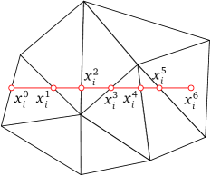
Figure 2: The path to calculate the left derivative. ($x_{i}^{0}=a(y_{i})$, $x_{i}^{6}=x_{i}$)

As long as we have found the intersection points, we can compute the value of ${}_{a(y)}D_{x}^{\alpha}\varphi_{l}|_{(x_{i},y_{i})}$ and ${}_{x}D_{b(y)}^{\alpha}\varphi_{k}|_{(x_{i},y_{i})}$. Take ${}_{a(y)}D_{x}^{\alpha}\varphi_{l}|_{(x_{i},y_{i})}$ as an example. Suppose the segment $y=y_{i},a(y_{i})\leq x\leq x_{i}$ intersects with edges of all triangles at $n_{i}$ points, and arrange them orderly like $x_{i}^{0}<x_{i}^{1}<x_{i}^{2}<\dots<x_{i}^{n_{i}}$, as show in Fig. 2. The value of ${}_{a(y)}D_{x}^{\alpha}\varphi_{l}|_{(x_{i},y_{i})}$ is

$${}_{a(y)}D_{x}^{\alpha}\varphi_{l}|_{(x_{i},y_{i})} ={}_{a(y_{i})}D_{x}^{\alpha}\varphi_{l}(x,y_{i})|_{x=x_{i}}$$ (20)

$$={\Big{(}\frac{1}{\Gamma(1-\alpha)}\frac{d}{dx}\int_{a(y_{i})}^{x}{(x-t)}^{-\alpha}\varphi_{l}(t,y_{i})\,dt\Big{)}}_{x=x_{i}}$$

$$=\sum^{n_{i}}_{j=1}{\Big{(}\frac{1}{\Gamma(1-\alpha)}\frac{d}{dx}\int_{x_{i}^{j-1}}^{x_{i}^{j}}{(x-t)}^{-\alpha}\varphi_{l}(t,y_{i})\,dt\Big{)}}_{x=x_{i}}$$

$$=\sum^{n_{i}}_{j=1}S_{j}\big{(}x;(x_{i},y_{i})\big{)}\big{|}_{x=x_{i}}.$$

where

$$S_{j}(x;(x_{i},y_{i}))=\frac{1}{\Gamma(1-\alpha)}\frac{d}{dx}\int_{x_{i}^{j-1}}^{x_{i}^{j}}{(x-t)}^{-\alpha}\varphi_{l}(t,y_{i})\,dt.$$ (21)

In the following, we demonstrate how to calculate $S_{j}(x;(x_{i},y_{i}))$. Integrating by parts, we notice the fact that

$$\frac{d}{dx}\int_{a}^{b}(x-t)^{-\alpha}f(t)\,dt= \ -f(t)(x-t)^{-\alpha}\big{|}_{t=a}^{t=b}$$ (22)

$$+\frac{1}{1-\alpha}\frac{d}{dx}\int_{a}^{b}(x-t)^{1-\alpha}f^{\prime}(t)\,dt,\quad x\notin[a,b],$$

and

$$\frac{d}{dx}\int_{a}^{x}(x-t)^{-\alpha}f(t)\,dt=f(a)(x-a)^{-\alpha}+\frac{1}{1-\alpha}\frac{d}{dx}\int_{a}^{x}(x-t)^{1-\alpha}f^{\prime}(t)\,dt.$$ (23)

when $f(x)\in C^{1}[a,b]$ and $\alpha<1$. It is obvious that basis function $\varphi_{l}(x,y_{i})$ is infinitely differentiable in $[x_{i}^{j-1},x_{i}^{j}]$ for fixed $y_{i}$. Define $f(x)=\varphi_{l}(x,y_{i})$, then $f(x)\in C^{\infty}[x_{i}^{j-1},x_{i}^{j}]$. Using formulas (22) and (23), we have

$$S_{j}(x;(x_{i},y_{i})) =\frac{1}{\Gamma(1-\alpha)}\frac{d}{dx}\int_{x_{i}^{j-1}}^{x_{i}^{j}}(x-t)^{-\alpha}f(t)\,dt$$ (24)

$$=\frac{-1}{\Gamma(1-\alpha)}f(t)(x-t)^{-\alpha}|_{t=x_{i}^{j-1}}^{t=x_{i}^{j}}+\frac{-1}{\Gamma(2-\alpha)}f^{\prime}(t)(x-t)^{1-\alpha}|_{t=x_{i}^{j-1}}^{t=x_{i}^{j}}$$

$$+\frac{1}{\Gamma(3-\alpha)}\frac{d}{dx}\int_{x_{i}^{j-1}}^{x_{i}^{j}}f^{\prime\prime}(t)(x-t)^{2-\alpha}\,dt\qquad(x_{i}^{j}\neq x,x\notin[x_{i}^{j-1},x_{i}^{j}]),$$

and

$$S_{j}(x;(x_{i},y_{i})) =\frac{1}{\Gamma(1-\alpha)}\frac{d}{dx}\int_{x_{i}^{j-1}}^{x}(x-t)^{\alpha}f(t)\,dt$$ (25)

$$=\frac{1}{\Gamma(1-\alpha)}f(x_{i}^{j-1})(x-x_{i}^{j-1})^{-\alpha}+\frac{1}{\Gamma(2-\alpha)}f^{\prime}(x_{i}^{j-1})(x-x_{i}^{j-1})^{1-\alpha}$$

$$+\frac{1}{\Gamma(3-\alpha)}\frac{d}{dx}\int_{x_{i}^{j-1}}^{x}f^{\prime\prime}(t)(x-t)^{2-\alpha}\,dt,\qquad(x_{i}^{j}=x).$$

If we use linear triangular element, i.e. $f(x)$ is linear function, then there are two terms in (24) without last line. So we can get the derivative by adding the value in all intervals.

4 Stability and convergence

In this section we analyze the stability and convergence of BEGM. In the following part, let $\lambda=\max\{\alpha,\beta\}$ and the constant $C$ may have different value in different context.

According to the bilinear form $a(u,v)$, we define seminorm $|\cdot|_{(\alpha,\beta)}$ and norm $\|\cdot\|_{(\alpha,\beta)}$ as follows[31]:

$$|u|_{(\alpha,\beta)} ={(K_{x}\|{}_{a(y)}D_{x}^{\alpha}u\|^{2}+K_{y}\|{}_{c(x)}D_{y}^{\beta}u\|^{2})}^{1/2},$$ (26)

$$\|u\|_{(\alpha,\beta)} ={(\|u\|^{2}+|u|_{(\alpha,\beta)}^{2})}^{1/2}.$$

where $\|\cdot\|=\|\cdot\|_{L_{2}(\Omega)}=\big{(}\int_{\Omega}|\cdot|^{2}dx\big{)}^{1/2}$. Due to Lemma 2.2, seminorm $|\cdot|_{(\alpha,\beta)}$ and norm $\|\cdot\|_{(\alpha,\beta)}$ are equivalent if $u\in H_{0}^{\alpha}(\Omega)\cap H_{0}^{\beta}(\Omega)$, which is described as the following lemma.

Lemma 4.1.

Suppose that $\Omega$ is convex domain, $u\in V$. Then there exists positive constants $C_{1}<1$ and $C_{2}$ independent of $u$, such that

$$C_{1}\|u\|_{(\alpha,\beta)}\leq|u|_{(\alpha,\beta)}\leq\|u\|_{(\alpha,\beta)}\leq C_{2}|u|_{H^{\lambda}(\Omega)}.$$ (27)

Proof.

From Lemma 2.2, we immediately have

$$\|u\|\leq C|u|_{(\alpha,\beta)},$$

where $C$ is independent of $u$. Therefore, there exists positive constants $C_{1}<1$ independent of $u$, such that

$$C_{1}\|u\|_{(\alpha,\beta)}\leq|u|_{(\alpha,\beta)},\quad C_{1}=\frac{1}{\sqrt{C^{2}+1}}$$ (28)

The inequality $|u|_{(\alpha,\beta)}\leq\|u\|_{(\alpha,\beta)}$ is obvious from their definitions. Using Lemma 2.2 again, we find

$$|u|_{(\alpha,\beta)}\leq C|u|_{J_{L}^{\lambda}(\Omega)}.$$ (29)

Combining inequalities (28), (29) and Lemma 2.1, we have

$$\|u\|_{(\alpha,\beta)}\leq\frac{1}{C_{1}}|u|_{(\alpha,\beta)}\leq\frac{C}{C_{1}}|u|_{J_{L}^{\lambda}(\Omega)}\leq C_{2}|u|_{H^{\lambda}(\Omega)}.$$ (30)

The proof is completed. ∎

By Lemma 4.1, we can obtain the following properties of $a(u,v)$.

Theorem 4.2.

The bilinear form $a(u,v)$ is continuous and coercive, i.e.

$$a(u,v)\leq\mathcal{A}\|u\|_{(\alpha,\beta)}\|v\|_{(\alpha,\beta)},\medspace a(u,u)\geq\mathcal{B}\|u\|_{(\alpha,\beta)}^{2},\quad\forall u\in H_{0}^{\alpha}(\Omega)\cap H_{0}^{\beta}(\Omega),$$ (31)

where $\mathcal{A}$ and $\mathcal{B}$ are positive constants independent of $u$.

Proof.

According to the definition of $a(u,v)$ and Cauchy-Schwarz inequality, we have

$$a(u,v) \leq K_{x}|c_{\alpha}|\|{}_{a(y)}D_{x}^{\alpha}u\|\|{}_{x}D_{b(y)}^{\alpha}v\|+K_{y}|c_{\beta}|\|{}_{c(x)}D_{y}^{\beta}u\|\|{}_{y}D_{d(x)}^{\beta}v\|$$ (32)

$$\quad+K_{x}|c_{\alpha}|\|{}_{x}D_{b(y)}^{\alpha}u\|\|{}_{a(y)}D_{x}^{\alpha}v\|+K_{y}|c_{\beta}|\|{}_{y}D_{d(x)}^{\beta}u\|\|{}_{c(x)}D_{y}^{\beta}v\|$$

Then by inequality

$$a_{1}b_{1}+a_{2}b_{2}\leq\sqrt{a_{1}^{2}+a_{2}^{2}}\sqrt{b_{1}^{2}+b_{2}^{2}},\quad a_{1},b_{1},a_{2},b_{2}>0,$$

we can obtain

$$a(u,v) \leq C|u|_{(\alpha,\beta)}\sqrt{K_{x}\|{}_{x}D_{b(y)}^{\alpha}v\|^{2}+K_{y}\|{}_{y}D_{d(x)}^{\beta}v\|^{2}}$$ (33)

$$\quad+C|v|_{(\alpha,\beta)}\sqrt{K_{x}\|{}_{x}D_{b(y)}^{\alpha}u\|^{2}+K_{y}\|{}_{y}D_{d(x)}^{\beta}u\|^{2}}$$

where $C=\max\{|c_{\alpha}|,|c_{\beta}|\}$. By Lemma 2.5, we know

$$\|{}_{x}D_{b(y)}^{\alpha}v\|^{2}\leq C_{1}\|{}_{a(y)}D_{x}^{\alpha}v\|^{2}$$ (34)

$$\|{}_{y}D_{d(x)}^{\beta}v\|^{2}\leq C_{2}\|{}_{c(x)}D_{y}^{\beta}v\|^{2}$$

where $C_{1},C_{2}$ are non-negative constants. Then, by Lemma 4.1, we have

$$a(u,v)\leq\mathcal{A}|u|_{(\alpha,\beta)}|v|_{(\alpha,\beta)}\leq\mathcal{A}\|u\|_{(\alpha,\beta)}\|v\|_{(\alpha,\beta)},$$ (35)

where $\mathcal{A}=2\max\{|c_{\alpha}|,|c_{\beta}|\}\sqrt{\max\{C_{1},C_{2}\}}$.

Let’s move on to the second inequality. From Lemma 2.3 and Lemma 4.1, we have

$$a(u,u) =2K_{x}c_{\alpha}({}_{a(y)}D_{x}^{\alpha}u,{}_{x}D_{b(y)}^{\alpha}u)+2K_{y}c_{\beta}({}_{c(x)}D_{y}^{\beta}u,{}_{y}D_{d(x)}^{\beta}u)$$ (36)

$$=K_{x}\|{}_{-\infty}D_{x}^{\mu}\hat{u}\|^{2}_{L^{2}(\mathbb{R}^{2})}+K_{y}\|{}_{-\infty}D_{y}^{\mu}\hat{u}\|^{2}_{L^{2}(\mathbb{R}^{2})}$$

$$\geq{K_{x}\|{}_{a(y)}D_{x}^{\alpha}u\|^{2}+K_{y}\|{}_{c(x)}D_{y}^{\beta}u\|^{2}},$$

$$=|u|_{(\alpha,\beta)}^{2}\geq\mathcal{B}\|u\|_{(\alpha,\beta)}^{2}.$$

Now we have proved the properties (31) of $a(u,v)$. ∎

Assume that $F(u)\in C^{1}(\Theta)$ with $M_{1}=\max\limits_{u\in\Theta}|F(u)|$, and $M_{2}=\max\limits_{u\in\Theta}|F^{\prime}(u)|$. In Eq. (14), let $v_{h}=u_{h}^{n}$, then

$$(u_{h}^{n},u_{h}^{n}) +\tau a(u_{h}^{n},u_{h}^{n})-\tau(F^{\prime}(u_{h}^{n-1})u_{h}^{n},u_{h}^{n})$$ (37)

$$=(u_{h}^{n-1},u_{h}^{n})+\tau(F(u_{h}^{n-1})-F^{\prime}(u_{h}^{n-1})u_{h}^{n-1},u_{h}^{n})+\tau(f^{n},u_{h}^{n}).$$

Using the property $a(u_{h}^{n},u_{h}^{n})\geq\mathcal{B}\|u_{h}^{n}\|^{2}_{(\alpha,\beta)}\geq\mathcal{B}\|u_{h}^{n}\|^{2}$ and Cauchy-Schwarz inequality yields

$$\|u_{h}^{n}\|^{2} +\tau(\mathcal{B}-M_{2})\|u_{h}^{n}\|^{2}\leq\|u_{h}^{n}\|\|u_{h}^{n-1}\|$$ (38)

$$+\tau M_{1}S\|u_{h}^{n}\|+\tau M_{2}\|u_{h}^{n}\|\|u_{h}^{n-1}\|+\tau\|f^{n}\|\|u_{h}^{n}\|,$$

where $S$ is the positive square root of the area of domain $\Omega$. Then

$$\|u_{h}^{n}\|+\tau(\mathcal{B}-M_{2})\|u_{h}^{n}\|\leq\|u_{h}^{n-1}\|+\tau M_{2}\|u_{h}^{n-1}\|+\tau\|f^{n}\|+\tau M_{1}S.$$ (39)

Summing $n$ from $1$ to $k$ in (39)

$$\|u_{h}^{k}\| +\tau(\mathcal{B}-M_{2})\|u_{h}^{k}\|\leq\|u_{h}^{0}\|+\tau M_{2}\|u_{h}^{0}\|$$ (40)

$$+\tau(2M_{2}-\mathcal{B})\sum\limits_{n=1}^{k-1}\|u_{h}^{n}\|+\tau\sum\limits_{n=1}^{k}\|f^{n}\|+k\tau M_{1}S.$$

In case $\mathcal{B}\geq M_{2}$, we see that

$$\|u_{h}^{k}\| \leq C\|u_{h}^{0}\|+\tau C\sum\limits_{n=1}^{k-1}\|u_{h}^{n}\|+\tau\sum\limits_{n=1}^{k}\|f^{n}\|+k\tau M_{1}S.$$ (41)

where $C$ is a non-negative constant independent with $u_{h}$. In case $\mathcal{B}<M_{2}$, let $\tau<\frac{1}{2(M_{2}-\mathcal{B})}$, then inequality (41) also holds.

To conduct analysis on stability, we make use of the following Grönwall inequality.

Lemma 4.3 ([32]).

Assume that $k_{n}$ is a nonnegative sequence, $g_{0}>0$, and the non-negative sequence $\{\varphi_{n}\}$ satisfies $\varphi_{0}\leq g_{0}$ and

$$\varphi_{n}\leq g_{0}+\sum\limits_{j=0}^{n-1}k_{j}\varphi_{j},\quad n\geq 1.$$ (42)

Then

$$\varphi_{n}\leq g_{0}\exp\Bigg{(}\sum\limits_{j=0}^{n-1}k_{j}\Bigg{)},\quad n\geq 1.$$ (43)

By Lemma 4.3 and inequality (41), we have

$$\|u_{h}^{k}\|\leq q_{k}\exp\left(\tau C(k-1)\right)\leq q_{n_{T}}\exp(CT),$$ (44)

where

$$q_{k}=C\|u_{h}^{0}\|+\tau\sum\limits_{n=1}^{k}\|f^{n}\|+k\tau M_{1}S.$$ (45)

So the analysis of stability is completed. In conclusion, we have proved the following theorem.

Theorem 4.4 (stability).

Suppose that $u_{h}^{n}$ are solutions of (14), and $F(x)$ satisfies $F(x)\in C^{1}(\Theta)$, $|F(x)|\leq M_{1}$, and $|F^{\prime}(x)|\leq M_{2}$. Assume $\tau<\frac{1}{2(M_{2}-\mathcal{B})}$ if $\mathcal{B}<M_{2}$. Then

$$\|u_{h}^{k}\|\leq q_{k}\exp\left(\tau C(k-1)\right)\leq q_{n_{T}}\exp(CT)$$ (46)

where $q_{k}$ is defined by (45).

Next, consider the convergence of BEGM. First, define projection operator $P_{h}:V\rightarrow V_{h}$ with following property:

$$a(u-P_{h}u,v_{h})=0,u\in V,\forall v_{h}\in V_{h}.$$ (47)

In order to exploit the property of the projection operator $P_{h}$, let us suppose that there is an interpolation $I_{h}:H^{s+1}(\Omega)\rightarrow V_{h}$ satisfied that

$$\|u-I_{h}u\|_{H^{\gamma}(\Omega)}\leq Ch^{\mu-\gamma}\|u\|_{H^{\mu}(\Omega)},\quad\forall u\in H^{\mu}(\Omega),\quad 0\leq\gamma<\mu\leq s+1.$$ (48)

Then we can deduce an approximation property of $P_{h}$.

Lemma 4.5.

If $u\in H^{\mu}(\Omega)\cap V$, $\lambda<\mu\leq s+1$, then the following estimate holds:

$$|u-P_{h}u|_{(\alpha,\beta)}\leq Ch^{\mu-\lambda}\|u\|_{H^{\mu}(\Omega)},$$ (49)

where $C$ is independent of $h$ and $u$.

The proof is similar with Lemma 4.4 in [31], so we omit here.

Let $\theta^{n}=u_{h}^{n}-P_{h}u^{n}$, $\rho^{n}=P_{h}u^{n}-u^{n}$, and $e^{n}=u_{h}^{n}-u^{n}=\theta^{n}+\rho^{n}$. The exact solution $u^{n}$ satisfies

$$(\partial_{t}u^{n},v_{h})+a(u^{n},v_{h})=\big{(}F(u^{n}),v_{h}\big{)}+(f^{n},v_{h}),\forall v_{h}\in V_{h},t\in(0,T].$$ (50)

And $u_{h}^{n}$ is the numerical solution of

$$(\bar{\partial}_{t}u_{h}^{n},v_{h})+a(u_{h}^{n},v_{h})=\big{(}F(u_{h}^{n-1}),v_{h}\big{)}+\big{(}F^{\prime}(u^{n-1}_{h})(u_{h}^{n}-u_{h}^{n-1}),v_{h}\big{)}+(f^{n},v_{h}),\forall v_{h}\in V_{h}.$$ (51)

Subtracting (50) from (51), we obtain

$$(\bar{\partial}_{t}e^{n},v_{h}) +a(e^{n},v_{h})=(u_{t}^{n}-\bar{\partial}_{t}u^{n},v_{h})$$ (52)

$$+\big{(}F(u_{h}^{n-1})-F(u^{n}),v_{h}\big{)}+\big{(}F^{\prime}(u^{n-1}_{h})(u_{h}^{n}-u_{h}^{n-1}),v_{h}\big{)}.$$

Firstly, we estimate $\|\theta^{n}\|_{(\alpha,\beta)}$. Since $a(\rho^{n},v_{h})=0$, the Eq. (52) can be written as

$$(\bar{\partial}_{t}\theta^{n},v_{h}) +a(\theta^{n},v_{h})=(u_{t}^{n}-\bar{\partial}_{t}u^{n},v_{h})-(\bar{\partial}_{t}\rho^{n},v_{h})$$ (53)

$$+\big{(}F(u_{h}^{n-1})-F(u^{n}),v_{h}\big{)}+\big{(}F^{\prime}(u^{n-1}_{h})(u_{h}^{n}-u_{h}^{n-1}),v_{h}\big{)}.$$

Let $v_{h}=\bar{\partial}_{t}\theta^{n}$ in (53), then

$$(\bar{\partial}_{t}\theta^{n},\bar{\partial}_{t}\theta^{n}) +a(\theta^{n},\bar{\partial}_{t}\theta^{n})=(u_{t}^{n}-\bar{\partial}_{t}u^{n},\bar{\partial}_{t}\theta^{n})-(\bar{\partial}_{t}\rho^{n},\bar{\partial}_{t}\theta^{n})$$ (54)

$$+\big{(}F(u_{h}^{n-1})-F(u^{n}),\bar{\partial}_{t}\theta^{n}\big{)}+\big{(}F^{\prime}(u^{n-1}_{h})(u_{h}^{n}-u_{h}^{n-1}),\bar{\partial}_{t}\theta^{n}\big{)}.$$

Separate $\theta^{n}$ from the right hand of (54) by Cauchy-Schwarz inequality

$$(u_{t}^{n}-\bar{\partial}_{t}u^{n},\bar{\partial}_{t}\theta^{n})\leq\frac{1}{2\varepsilon}\|u_{t}^{n}-\bar{\partial}_{t}u^{n}\|^{2}+\frac{\varepsilon}{2}\|\bar{\partial}_{t}\theta^{n}\|^{2},$$ (55)

$$(\bar{\partial}_{t}\rho^{n},\bar{\partial}_{t}\theta^{n})\leq\frac{1}{2\varepsilon}\|\bar{\partial}_{t}\rho^{n}\|^{2}+\frac{\varepsilon}{2}\|\bar{\partial}_{t}\theta^{n}\|^{2},$$ (56)

$$(F(u_{h}^{n-1})-F(u^{n}),\bar{\partial}_{t}\theta^{n}) \leq\|F(u_{h}^{n-1})-F(u^{n})\|\|\bar{\partial}_{t}\theta^{n}\|$$ (57)

$$\leq\|M_{2}(u_{h}^{n-1}-u^{n})\|\|\bar{\partial}_{t}\theta^{n}\|$$

$$\leq\frac{M_{2}^{2}}{2\varepsilon}\|u_{h}^{n-1}-u^{n}\|^{2}+\frac{\varepsilon}{2}\|\bar{\partial}_{t}\theta^{n}\|^{2},$$

$$(F^{\prime}(u^{n-1}_{h})(u_{h}^{n}-u_{h}^{n-1}),\bar{\partial}_{t}\theta^{n})\leq\frac{M_{2}^{2}}{2\varepsilon}\|u_{h}^{n-1}-u_{h}^{n}\|^{2}+\frac{\varepsilon}{2}\|\bar{\partial}_{t}\theta^{n}\|^{2}.$$ (58)

Let $\varepsilon=1/2$ in (55)-(58), then we see

$$a(\theta^{n},\theta^{n})-a(\theta^{n-1},\theta^{n-1}) \leq 2\tau\|u_{t}^{n}-\bar{\partial}_{t}u^{n}\|^{2}+2\tau\|\bar{\partial}_{t}\rho^{n}\|^{2}$$ (59)

$$+2\tau M_{2}^{2}\|u_{h}^{n-1}-u^{n}\|^{2}+2\tau M_{2}^{2}\|u_{h}^{n-1}-u_{h}^{n}\|^{2},$$

where we have used the following equality,

$$a(\theta^{n},\bar{\partial}_{t}\theta^{n})=\frac{1}{2\tau}\left(a(\theta^{n},\theta^{n})+a(\theta^{n}-\theta^{n-1},\theta^{n}-\theta^{n-1})-a(\theta^{n-1},\theta^{n-1})\right).$$ (60)

Also note that the last two terms in (59) can be estimated as

$$\left\{\begin{aligned} &\|u_{h}^{n-1}-u^{n}\|^{2}\leq 3(\|\rho^{n-1}\|^{2}+\|\theta^{n-1}\|^{2}+\|u^{n-1}-u^{n}\|^{2}),\\ &\|u_{h}^{n-1}-u_{h}^{n}\|^{2}\leq 5(\|\rho^{n-1}\|^{2}+\|\theta^{n-1}\|^{2}+\|\rho^{n}\|^{2}+\|\theta^{n}\|^{2}+\|u^{n-1}-u^{n}\|^{2}),\end{aligned}\right.$$ (61)

here we have used the Minkowski inequality and

$$(a_{1}+a_{2}+\cdots+a_{m})^{2}\leq m(a_{1}^{2}+a_{2}^{2}+\cdots+a_{m}^{2}),$$ (62)

where $a_{i}(i=1,\cdots,m)$ is non-negative real number. The inequalities (59), (61) and the fact $a(\theta^{k},\theta^{k})\geq\mathcal{B}\|\theta^{k}\|_{(\alpha,\beta)}^{2}$ yield

$$\mathcal{B}\|\theta^{k}\|_{(\alpha,\beta)}^{2} \leq a(\theta^{0},\theta^{0})+2\tau\sum\limits_{n=1}^{k}(\|u_{t}^{n}-\bar{\partial}_{t}u^{n}\|^{2}+\|\bar{\partial}\rho^{n}\|^{2})$$ (63)

$$+2\tau M_{2}^{2}\Big{(}5\|\theta^{k}\|^{2}+13\sum\limits_{n=0}^{k}\|\rho^{n}\|^{2}+13\sum\limits_{n=0}^{k-1}\|\theta^{n}\|^{2}+13\sum\limits_{n=1}^{k}\|u^{n-1}-u^{n}\|^{2}\Big{)}.$$

When $\tau\leq\frac{\mathcal{B}}{20M_{2}^{2}}$, we have

$$\|\theta^{k}\|_{(\alpha,\beta)}^{2}\leq Cg_{k}+\tau C^{\prime}M_{2}^{2}\sum\limits_{n=0}^{k-1}\|\theta^{n}\|_{(\alpha,\beta)}^{2}$$ (64)

where $C=\frac{1}{\mathcal{B}-10\tau M_{2}^{2}}$, $C^{\prime}=\frac{26}{\mathcal{B}-10\tau M_{2}^{2}}$, and $g_{k}$ is defined as

$$g_{k}= a(\theta^{0},\theta^{0})+2\tau\sum\limits_{n=1}^{k}(\|u_{t}^{n}-\bar{\partial}_{t}u^{n}\|^{2}+\|\bar{\partial}\rho^{n}\|^{2})$$ (65)

$$+26\tau M_{2}^{2}\Big{(}\sum\limits_{n=0}^{k}\|\rho^{n}\|^{2}+\sum\limits_{n=1}^{k}\|u^{n-1}-u^{n}\|^{2}\Big{)}.$$

By Lemma 4.3 and inequality (64), the following estimation holds

$$\|\theta^{k}\|_{(\alpha,\beta)}^{2}\leq Cg_{k}\exp{(C^{\prime}TM_{2}^{2})}.$$ (66)

Now, we need to estimate $g_{k}$. In order to make it clear, we denote $\|\cdot\|_{\mu}=\|\cdot\|_{H^{\mu}(\Omega)}$ and $\|\cdot\|_{0,\mu}=(\int_{0}^{T}\|\cdot\|^{2}_{\mu}dt)^{1/2}.$ The continuity of $a(u,v)$ and Lemma 4.5 imply that

$$a(\theta^{0},\theta^{0}) \leq C\|\theta^{0}\|_{(\alpha,\beta)}^{2}\leq C\left(\|u^{0}_{h}-u(t_{0})\|^{2}_{\lambda}+\|u(t_{0})-P_{h}u(t_{0})\|^{2}_{(\alpha,\beta)}\right)$$ (67)

$$\leq C\left(\|u^{0}_{h}-u(t_{0})\|^{2}_{\lambda}+h^{2\mu-2\lambda}\|u(t_{0})\|^{2}_{\mu}\right).$$

For the term with $\|u_{t}^{n}-\bar{\partial}_{t}u^{n}\|$, we use Taylor formula and Cauchy-Schwarz inequality:

$$u_{t}^{n}-\bar{\partial}_{t}u^{n} =\frac{1}{\tau}\int_{t_{n-1}}^{t_{n}}(t-t_{n-1})u_{tt}dt$$ (68)

$$\leq\frac{1}{\tau}{\bigg{(}\int_{t_{n-1}}^{t_{n}}{(t-t_{n-1})}^{2}dt\int_{t_{n-1}}^{t_{n}}u_{tt}^{2}dt\bigg{)}}^{\frac{1}{2}}$$

$$={\left(\frac{\tau}{3}\right)}^{\frac{1}{2}}{\bigg{(}\int_{t_{n-1}}^{t_{n}}u_{tt}^{2}dt\bigg{)}}^{\frac{1}{2}}.$$

Then we have

$$2\tau\sum\limits_{n=1}^{k}\|u_{t}^{n}-\bar{\partial}_{t}u^{n}\|^{2}\leq 2\tau\sum\limits_{n=1}^{k}\int_{\Omega}\bigg{(}\frac{\tau}{3}\int_{t_{n-1}}^{t_{n}}u_{tt}^{2}dt\bigg{)}dxdy=\frac{2\tau^{2}}{3}\|u_{tt}\|^{2}_{0,0}.$$ (69)

Apply Cauchy-Schwarz inequality to the third term of $g_{k}$, then we obtain

$$2\tau\sum\limits_{n=1}^{k}\|\bar{\partial}_{t}\rho^{n}\|^{2} =2\tau\sum\limits_{n=1}^{k}\|\frac{1}{\tau}\int_{t_{n-1}}^{t_{n}}\rho_{t}dt\|^{2}$$ (70)

$$\leq 2\tau\sum\limits_{n=1}^{k}\int_{\Omega}\bigg{(}\frac{1}{\tau^{2}}\int_{t_{n-1}}^{t_{n}}1^{2}dt\int_{t_{n-1}}^{t_{n}}\rho_{t}^{2}dt\bigg{)}dxdy$$

$$\leq Ch^{2\mu-2\lambda}\|u_{t}\|_{0,\mu}^{2}.$$

By the definition of $\rho^{n}$ and the property of projection $P_{h}$, we have

$$6\tau M_{2}^{2}\sum\limits_{n=0}^{k}\|\rho^{n}\|^{2} \leq 6\tau M_{2}^{2}\sum\limits_{n=0}^{k}\|\rho^{n}\|_{(\alpha,\beta)}^{2}$$ (71)

$$\leq 6\tau M_{2}^{2}\sum\limits_{n=0}^{k}Ch^{2\mu-2\lambda}\|u^{n}\|_{\mu}^{2}$$

$$\leq CTM_{2}^{2}h^{2\mu-2\lambda}\max\limits_{t_{0}\leq t\leq T}\|u(t)\|_{\mu}^{2}.$$

For the last term of $g_{k}$, we use Cauchy-Schwarz inequality again:

$$2\tau M_{2}^{2}\sum\limits_{n=1}^{k}\|u^{n-1}-u^{n}\|^{2} =2\tau M_{2}^{2}\sum\limits_{n=1}^{k}\int_{\Omega}{\bigg{(}\int_{t_{n-1}}^{t_{n}}u_{t}dt\bigg{)}}^{2}dxdy$$ (72)

$$\leq 2\tau^{2}M_{2}^{2}\int_{\Omega}\left(\int_{t_{0}}^{t_{n_{T}}}u_{t}^{2}dt\right)dxdy$$

$$=2\tau^{2}M_{2}^{2}\|u_{t}\|^{2}_{0,0}.$$

Hence, $g_{k}$ can be estimated as

$$g_{k}\leq C\|u^{0}_{h}-u(t_{0})\|^{2}_{\lambda}+C\tau^{2}\big{(}\|u_{tt}\|^{2}_{0,0}+M_{2}^{2}\|u_{t}\|^{2}_{0,0}\big{)}$$ (73)

$$+Ch^{2\mu-2\lambda}\big{(}\|u(t_{0})\|^{2}_{\mu}+\|u_{t}\|_{0,\mu}^{2}+TM_{2}^{2}\max_{0\leq t\leq T}\|u(t)\|_{\mu}^{2}\big{)}.$$

Since $u_{h}^{k}-u^{k}=\theta^{k}+\rho^{k}$, we have the result

$$\|u_{h}^{k}-u^{k}\|_{(\alpha,\beta)}^{2} \leq C(\|\theta^{k}\|_{(\alpha,\beta)}^{2}+\|\rho^{k}\|_{(\alpha,\beta)}^{2})$$ (74)

$$\leq Cg_{k}\exp(C^{\prime}TM_{2}^{2})+Ch^{2\mu-2\lambda}\|u(t_{k})\|^{2}_{\mu}$$

$$\leq C\exp(C^{\prime}TM_{2}^{2})\Big{(}\|u^{0}_{h}-u(t_{0})\|^{2}_{\lambda}+\tau^{2}\left(\|u_{tt}\|^{2}_{0,0}+M_{2}^{2}\|u_{t}\|^{2}_{0,0}\right)$$

$$+h^{2\mu-2\lambda}\big{(}\|u(t_{0})\|^{2}_{\mu}+\|u(t_{k})\|^{2}_{\mu}+\|u_{t}\|_{0,\mu}^{2}+TM_{2}^{2}\max_{0\leq t\leq T}\|u(t)\|_{\mu}^{2}\big{)}\Big{)}$$

When choosing the interpolation as initial value of $u$ at time $t_{0}$, i.e. $u_{h}^{0}=I_{h}u(t_{0})$, the following inequality holds

$$\|u_{h}^{k}-u^{k}\|_{(\alpha,\beta)}^{2} \leq C\exp(C^{\prime}TM_{2}^{2})\Big{(}\tau^{2}\left(\|u_{tt}\|^{2}_{0,0}+M_{2}^{2}\|u_{t}\|^{2}_{0,0}\right)$$ (75)

$$+h^{2\mu-2\lambda}\big{(}\|u(t_{0})\|^{2}_{\mu}+\|u(t_{k})\|^{2}_{\mu}+\|u_{t}\|_{0,\mu}^{2}+TM_{2}^{2}\max_{0\leq t\leq T}\|u(t)\|_{\mu}^{2}\big{)}\Big{)}.$$

We finish the analysis of convergence of BEGM. The convergence theorem is shown below as a conclusion.

Theorem 4.6 (convergence).

Suppose that

1. $u_{h}^{n}$ are solutions of Eq. (14),

2. $F(x)\in C^{1}(\Theta)$, $|F(x)|\leq M_{1}$, and $|F^{\prime}(x)|\leq M_{2}$.

3. The exact solution $u\in L^{\infty}(0,T;H_{0}^{\mu}(\Omega))$, $u_{t}\in L^{2}(0,T;H_{0}^{\mu})$, and $u_{tt}\in L^{2}(0,T;L^{2}(\Omega))$, where $\lambda<\mu\leq s+1$.

Also assume $\tau<\frac{\mathcal{B}}{20M_{2}^{2}}$. Then we have

$$\|u_{h}^{k}- u^{k}\|_{(\alpha,\beta)}^{2}\leq C\tau^{2}\left(\|u_{tt}\|^{2}_{0,0}+\|u_{t}\|^{2}_{0,0}\right)$$ (76)

$$+Ch^{2\mu-2\lambda}\big{(}\|u(t_{0})\|^{2}_{\mu}+\|u(t_{k})\|^{2}_{\mu}+\|u_{t}\|_{0,\mu}^{2}+TM_{2}^{2}\max_{0\leq t\leq T}\|u(t)\|_{\mu}^{2}\big{)}.$$

Remark 4.7.

In Theorem 4.6, $\mu$ is related with smoothness of the exact solution $u$ and with the element type used in simulation. If we use linear triangular element in numerical examples, the degree of polynomials in space $V_{h}$ is at most $1$, i.e. $s=1$, then $\lambda<\mu\leq 2$. When the exact solution $u$ is good enough, we can get $\mu=2$, then the space convergence order is $2-\lambda$.

5 Numerical examples

In this section, we consider some numerical examples to demonstrate the effectiveness of our theoretical analysis. Here, linear triangular element is used.

Example 5.1.

Consider the following fractional problem

$$\left\{\begin{aligned} &\frac{\partial u}{\partial t}=K_{x}\frac{\partial^{2\alpha}u}{\partial|x|^{2\alpha}}+K_{y}\frac{\partial^{2\beta}u}{\partial|y|^{2\beta}}+F(u)+f(x,y,t),\\ &u(x,y,0)=\varphi(x,y),\quad(x,y)\in\Omega,\\ &u(x,y,t)=0,\quad(x,y,t)\in\partial\Omega\times(0,T],\end{aligned}\right.$$ (77)

where $\Omega=(0,1)\times(0,1)$, $F(u)=-u^{2}$, $\varphi(x,y)=10x^{2}{(1-x)}^{2}y^{2}{(1-y)}^{2}$, and

$$f(x,y,t)= -10e^{-t}x^{2}{(1-x)}^{2}y^{2}{(1-y)}^{2}+100e^{-2t}x^{4}{(1-x)}^{4}y^{4}{(1-y)}^{4}$$ (78)

$$+10K_{x}c_{\alpha}e^{-t}y^{2}(1-y)^{2}\big{(}g(x,\alpha)+g(1-x,\alpha)\big{)}$$

$$+10K_{y}c_{\beta}e^{-t}x^{2}(1-x)^{2}\big{(}g(y,\beta)+g(1-y,\beta)\big{)},$$

$$g(x,\alpha)=\frac{\Gamma(5)}{\Gamma(5-2\alpha)}x^{4-2\alpha}-\frac{2\Gamma(4)}{\Gamma(4-2\alpha)}x^{3-2\alpha}+\frac{\Gamma(3)}{\Gamma(3-2\alpha)}x^{2-2\alpha}.$$ (79)

The exact solution of Eq. (77) is

$$u(x,y,t)=10e^{-t}x^{2}{(1-x)}^{2}y^{2}{(1-y)}^{2}.$$

In this example, we take $K_{x}=K_{y}=1$, $T=1$ and compute the numerical results by different $\alpha$ and $\beta$. Two meshes used in computation are shown in Fig. 3. The results are given in Table 5.1. As we use linear triangular element, the spatial convergence order should be $2-\max\{\alpha,\beta\}$. By examining the rates of convergence shown in Table 5.1, we notice that the spatial convergence orders fit those proved in Theorem 4.6. The temporal convergence order for different norms are given in Table 2. As we can see, the convergence order of norm $||\cdot||_{(\alpha,\beta)}$ is close to 1. These results agree with the result of theoretical analysis. Besides, we plot numerical and exact solutions at $T=1$ with $h\approx 1/40$ in Fig. 4, which indicates that the numerical result is a good approximation of exact solution.

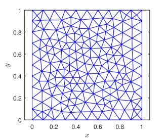
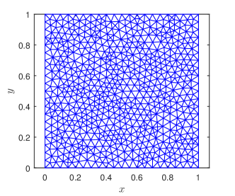
Figure 3: Meshes on rectangle domain with $h\approx 1/10$ and $h\approx 1/20$.

Table 1: Errors and space convergence orders of BEGM for Example 5.1 ($\tau=h^{2}$).

	h	$L^{2}$ error	Order	$L^{\infty}$ error	Order	$L^{(\alpha,\beta)}$ error	Order
$\alpha=0.8$ $\beta=0.8$	1/5	5.01e-04		6.19e-04		1.18e-03
	1/10	1.43e-04	1.81	1.49e-04	2.06	4.86e-04	1.29
	1/20	3.91e-05	1.87	6.25e-05	1.25	2.20e-04	1.14
	1/40	1.04e-05	1.91	1.95e-05	1.68	1.05e-04	1.06
$\alpha=0.95$ $\beta=0.95$	1/5	5.50e-04		8.57e-04		2.01e-03
	1/10	1.59e-04	1.79	1.86e-04	2.21	9.02e-04	1.16
	1/20	4.33e-05	1.87	6.97e-05	1.41	4.28e-04	1.08
	1/40	1.10e-05	1.98	2.07e-05	1.75	1.90e-04	1.17
$\alpha=0.8$ $\beta=0.75$	1/5	4.97e-04		6.02e-04		1.08e-03
	1/10	1.42e-04	1.81	1.47e-04	2.03	4.50e-04	1.26
	1/20	3.94e-05	1.85	7.46e-05	0.98	2.10e-04	1.10
	1/40	1.06e-05	1.89	2.06e-05	1.86	1.03e-04	1.03

Table 2: Errors and temporal convergence orders of BEGM for Example 5.1 with $\alpha=0.85$, $\beta=0.85$ ($h=\tau$).

$\tau$	$L^{2}$ error	Order	$L^{\infty}$ error	Order	$L^{(\alpha,\beta)}$ error	Order
1/5	4.72e-04		5.60e-04		1.31e-03
1/10	1.38e-04	1.77	1.69e-04	1.73	5.84e-04	1.17
1/20	3.76e-05	1.88	6.91e-05	1.29	2.70e-04	1.11
1/40	9.76e-06	1.94	2.09e-05	1.73	1.22e-04	1.15

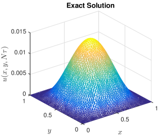
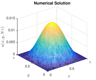
Figure 4: The exact solution and numerical approximation when $T=1$, $h\approx 1/40$ on rectangle domain.

Example 5.2.

Consider the following fractional problem

$$\left\{\begin{aligned} &\frac{\partial u}{\partial t}=K_{x}\frac{\partial^{2\alpha}u}{\partial|x|^{2\alpha}}+K_{y}\frac{\partial^{2\beta}u}{\partial|y|^{2\beta}}+F(u)+f(x,y,t),\\ &u(x,y,0)=\varphi(x,y),\quad(x,y)\in\Omega,\\ &u(x,y,t)=0,\quad(x,y,t)\in\partial\Omega\times(0,T],\end{aligned}\right.$$ (80)

where the domain $\Omega$ is shown in Fig. 5, $F(u)=-u^{2}$, $\varphi(x,y)=1000x^{2}{(1-x)}^{2}(x+y-1.5)^{2}y^{2}{(1-y)}^{2}$, and

$$f(x,y,t)= -1000e^{-t}x^{2}{(1-x)}^{2}(x+y-1.5)^{2}y^{2}{(1-y)}^{2}$$ (81)

$$+10^{6}e^{-2t}x^{4}{(1-x)}^{4}(x+y-1.5)^{4}y^{4}{(1-y)}^{4}$$

$$+1000e^{-t}K_{x}c_{\alpha}y^{2}(1-y)^{2}g(x,y,\alpha)$$

$$+1000e^{-t}K_{y}c_{\beta}x^{2}(1-y)^{2}g(y,x,\beta),$$

$$g(x,y,\alpha)=\left\{\begin{aligned} &g_{0}(x,1.5-y,\alpha)+g_{1}(1-x,1.5-y,\alpha),&&y\leq 0.5,\\ &g_{0}(x,1.5-y,\alpha)+g_{2}(1.5-y-x,1.5-y,\alpha),&&y>0.5,\end{aligned}\right.$$ (82)

$$g_{0}(x,y,\alpha)= \ \frac{2y^{2}x^{2-2\alpha}}{\Gamma(3-2\alpha)}-\frac{12\left(y^{2}-y\right)x^{3-2\alpha}}{\Gamma(4-2\alpha)}+\frac{24\left(y^{2}+4y+1\right)x^{4-2\alpha}}{\Gamma(5-2\alpha)}$$ (83)

$$-\frac{240(y+1)x^{5-2\alpha}}{\Gamma(6-2\alpha)}+\frac{720x^{6-2\alpha}}{\Gamma(7-2\alpha)},$$

$$g_{1}(x,y,\alpha)= \ \frac{2\left(y^{2}-2y+1\right)x^{2-2\alpha}}{\Gamma(3-2\alpha)}-\frac{12\left(y^{2}-3y+2\right)x^{3-2\alpha}}{\Gamma(4-2\alpha)}$$ (84)

$$+\frac{24\left(y^{2}-6y+6\right)x^{4-2\alpha}}{\Gamma(5-2\alpha)}+\frac{240(y-2)x^{5-2\alpha}}{\Gamma(6-2\alpha)}+\frac{720x^{6-2\alpha}}{\Gamma(7-2\alpha)},$$

$$g_{2}(x,y,\alpha)= \ \frac{2\left(y^{4}-2y^{3}+y^{2}\right)x^{2-2\alpha}}{\Gamma(3-2\alpha)}-\frac{12\left(2y^{3}-3y^{2}+y\right)x^{3-2\alpha}}{\Gamma(4-2\alpha)}$$ (85)

$$+\frac{24\left(6y^{2}-6y+1\right)x^{4-2\alpha}}{\Gamma(5-2\alpha)}+\frac{240(1-2y)x^{5-2\alpha}}{\Gamma(6-2\alpha)}+\frac{720x^{6-2\alpha}}{\Gamma(7-2\alpha)},$$

The exact solution of Eq. (80) is u(x,y,t)=1000e^-tx^2(1-x)^2(x+y-1.5)^2y^2(1-y)^2.

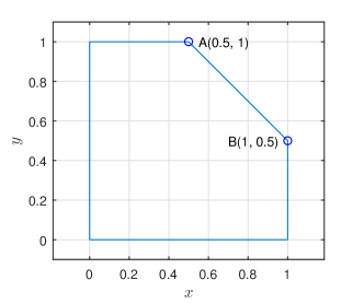
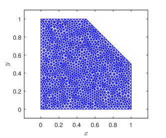
Figure 5: Poly domain and mesh with $h\approx 1/30$.

Table 3: Errors and spatial convergence orders of BEGM for Example 5.2($\tau=h^{2}$).

	h	$L^{2}$ error	Order	$L^{\infty}$ error	Order	$L^{(\alpha,\beta)}$ error	Order
$\alpha=0.8$ $\beta=0.8$	1/5	2.26e-02		2.66e-02		6.77e-02
	1/10	7.76e-03	1.54	1.30e-02	1.04	3.50e-02	0.95
	1/20	2.24e-03	1.79	5.37e-03	1.27	1.54e-02	1.19
	1/30	9.47e-04	2.13	2.84e-03	1.57	9.32e-03	1.23
$\alpha=0.95$ $\beta=0.95$	1/5	2.51e-02		3.73e-02		1.20e-01
	1/10	8.41e-03	1.58	1.41e-02	1.40	6.45e-02	0.90
	1/20	2.46e-03	1.77	6.50e-03	1.12	3.05e-02	1.08
	1/30	1.03e-03	2.14	3.55e-03	1.49	1.89e-02	1.17
$\alpha=0.8$ $\beta=0.7$	1/5	2.24e-02		2.59e-02		5.32e-02
	1/10	7.67e-03	1.55	1.12e-02	1.21	2.81e-02	0.92
	1/20	2.27e-03	1.76	4.50e-03	1.31	1.25e-02	1.17
	1/30	9.67e-04	2.10	2.30e-03	1.65	7.62e-03	1.23

Table 4: Errors and temporal convergence orders of BEGM for Example 5.2 with $\alpha=0.8$, $\beta=0.9$ ($h=\tau$).

$\tau$	$L^{2}$ error	Order	$L^{\infty}$ error	Order	$L^{(\alpha,\beta)}$ error	Order
1/10	7.98e-03		1.49e-02		4.92e-02
1/20	2.25e-03	1.83	6.75e-03	1.14	2.28e-02	1.11
1/30	9.64e-04	2.09	3.85e-03	1.38	1.44e-02	1.14
1/40	5.71e-04	1.82	2.48e-03	1.54	1.05e-02	1.08

In this test, we take $K_{x}=1,K_{y}=2$, $T=1$. We compute the $L^{2}(\Omega)$ errors, the $L^{\infty}(\Omega)$ errors, the $||\cdot||_{(\alpha,\beta)}$ errors, and the spatial convergence orders. Fig. 5 shows the mesh used in computation with $h\approx 1/16$. The results are given in Table 5.2. As shown in the table, the numerical results agree well with Theorem 4.6. We also give the temporal convergence order in Table 4. As we can see from the table, the numerical orders of $L^{(\alpha,\beta)}$ error agree well with the analysis result. Also, we plot numerical and exact solutions at $T=1$ with $h\approx 1/30$ in Fig. 6, which appears that the numerical result is a good approximation of the exact solution.

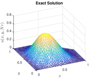
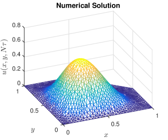
Figure 6: The exact solution and numerical approximation when $T=1$, $h\approx 1/30$ on poly domain.

Example 5.3.

Consider the following fractional model

$$\left\{\begin{aligned} &\frac{\partial u}{\partial t}=K_{x}\frac{\partial^{2\alpha}u}{\partial|x|^{2\alpha}}+K_{y}\frac{\partial^{2\beta}u}{\partial|y|^{2\beta}}+F(u)+f(x,y,t),\\ &u(x,y,0)=\varphi(x,y),\quad(x,y)\in\Omega,\\ &u(x,y,t)=0,\quad(x,y,t)\in\partial\Omega\times(0,T],\end{aligned}\right.$$ (86)

where $\Omega=\{(x,y):\frac{x^{2}}{a^{2}}+\frac{y^{2}}{b^{2}}<1\}$, $a>0$, $b>0$, $F(u)=-u^{2}$, $\varphi(x,y)=100\left(b^{2}x^{2}+a^{2}y^{2}-a^{2}b^{2}\right)^{2}$, and

$$f(x,y,t)= -100e^{-t}{(x^{2}+y^{2}-r^{2})}^{2}+10^{4}e^{-2t}{(x^{2}+y^{2}-r^{2})}^{4}$$ (87)

$$+100K_{x}c_{\alpha}e^{-t}h(x+a\sqrt{1-{y^{2}}/{b^{2}}},-\sqrt{1-{y^{2}}/{b^{2}}})$$

$$+100K_{x}c_{\alpha}e^{-t}h(a\sqrt{1-{y^{2}}/{b^{2}}}-x,\sqrt{1-{y^{2}}/{b^{2}}})$$

$$+100K_{y}c_{\beta}e^{-t}g(-\sqrt{1-{x^{2}}/{a^{2}}},y+b\sqrt{1-{x^{2}}/{a^{2}}})$$

$$+100K_{y}c_{\beta}e^{-t}g(\sqrt{1-{x^{2}}/{a^{2}}},b\sqrt{1-{x^{2}}/{a^{2}}}-y)$$

$$h(x,y)=\frac{8a^{2}b^{4}y^{2}x^{2-2\alpha}}{\Gamma(3-2\alpha)}+\frac{24ab^{4}yx^{3-2\alpha}}{\Gamma(4-2\alpha)}+\frac{24b^{4}x^{4-2\alpha}}{\Gamma(5-2\alpha)}$$ (88)

$$g(x,y)=\frac{8a^{4}b^{2}x^{2}y^{2-2\beta}}{\Gamma(3-2\beta)}+\frac{24a^{4}bxy^{3-2\beta}}{\Gamma(4-2\beta)}+\frac{24a^{4}y^{4-2\beta}}{\Gamma(5-2\beta)}$$ (89)

The exact solution to Eq. (86) is u(x,y,t)=100e^-t(b^2 x^2+a^2 y^2-a^2 b^2)^2.

In this example, set $a=1/2$, $b=3/4$, then the domain is an ellipse. Choose parameters $K_{x}=2$, $K_{y}=2$, $T=1$. Table 5.3 shows the spatial convergence orders. As $\alpha$, $\beta$ increase, the convergence order of $||\cdot||_{(\alpha,\beta)}$ errors decrease and the orders are close to $2-\max\{\alpha,\beta\}$. These results agree well with what we have proved in Theorem 4.6. For the temporal direction, we give the results in Table 6. Fig. 7 presents the computational domain and the mesh used in this example with $h\approx 1/30$ and Fig. 8 gives a comparison between exact solution and numerical solution. These results shows that our algorithm also works well in elliptical domain.

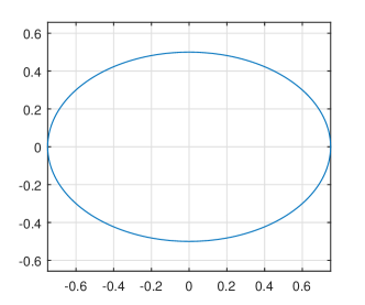
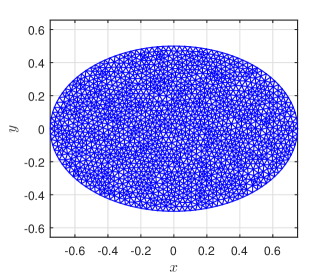
Figure 7: Elliptical domain and mesh with $h\approx 1/30$.

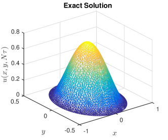
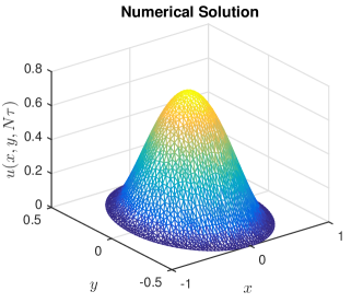
Figure 8: The exact solution and numerical approximation when $T=1$, $h\approx 1/30$ on elliptical domain.

Table 5: Errors and space convergence orders of BEGM for Example 5.3 ($\tau=h^{2}$).

	h	$L^{2}$ error	Order	$L^{\infty}$ error	Order	$L^{(\alpha,\beta)}$ error	Order
$\alpha=0.85$ $\beta=0.85$	1/5	2.80e-02		2.45e-02		9.63e-02
	1/10	7.73e-03	1.85	8.93e-03	1.46	4.38e-02	1.14
	1/20	2.02e-03	1.93	3.14e-03	1.51	1.89e-02	1.21
	1/30	9.15e-04	1.96	1.55e-03	1.75	1.21e-02	1.11
$\alpha=0.95$ $\beta=0.95$	1/5	3.06e-02		3.08e-02		1.40e-01
	1/10	8.32e-03	1.88	9.52e-03	1.70	6.68e-02	1.07
	1/20	2.18e-03	1.93	3.43e-03	1.47	2.99e-02	1.16
	1/30	9.79e-04	1.97	1.70e-03	1.74	1.91e-02	1.10
$\alpha=0.8$ $\beta=0.75$	1/5	2.74e-02		2.26e-02		7.97e-02
	1/10	7.69e-03	1.83	8.87e-03	1.35	3.36e-02	1.25
	1/20	2.03e-03	1.92	3.11e-03	1.51	1.48e-02	1.18
	1/30	9.37e-04	1.91	1.71e-03	1.48	1.01e-02	0.94

Table 6: Errors and temporal convergence orders of BEGM for Example 5.3 with $\alpha=0.85$, $\beta=0.85$ ($h=\tau$).

$\tau$	$L^{2}$ error	Order	$L^{\infty}$ error	Order	$L^{(\alpha,\beta)}$ error	Order
1/5	1.04e-02		8.70e-03		3.63e-02
1/10	2.95e-03	1.82	3.65e-03	1.25	1.73e-02	1.07
1/20	7.69e-04	1.94	1.29e-03	1.51	7.56e-03	1.19
1/30	3.40e-04	2.01	6.33e-04	1.75	4.83e-03	1.10

Example 5.4.

Consider the fractional FitzHugh-Nagumo problem

$$\left\{\begin{aligned} &\frac{\partial u}{\partial t}=K_{x}\frac{\partial^{2\alpha}u}{\partial|x|^{2\alpha}}+K_{y}\frac{\partial^{2\beta}u}{\partial|y|^{2\beta}}+u(1-u)(u-\mu)-w,\\ &\frac{\partial w}{\partial t}=\epsilon(\lambda u-\gamma w-\delta),\quad(x,y,t)\in\partial\Omega\times T,\\ &\Omega=\{(x,y):(x-r)^{2}+(y-r)^{2}<r^{2}\},\end{aligned}\right.$$ (90)

where $r=1.25$, $\mu=0.1$, $\epsilon=0.01$, $\lambda=0.5$, $\gamma=0.1$, $\delta=0$. The initial conditions are taken as

$$u(x,y,0)=\left\{\begin{aligned} 1,&\quad x<r,y<r\\ 0,&\quad elsewhere\end{aligned}\right.,\quad w(x,y,0)=\left\{\begin{aligned} 0.1,&\quad y\geq r\\ 0,&\quad elsewhere\end{aligned}\right.,$$ (91)

and the boundary conditions are homogeneous. For this coupled differential equation, we first solve the fractional Riesz space nonlinear equation by given $w$ and $u$, then solve the ordinary differential equation with $w$ and new $u$ at each time step.

The simulation results with $K_{x}=K_{y}=0.0001$ and $K_{x}=4K_{y}=0.00025$ at $T=1000$ are show in Fig. 9 and Fig. 10, respectively. From Fig. 9, we notice that as fractional orders $\alpha,\beta$ decrease, the wave travels more slowly. Fig. 10 shows anisotropic diffusion with different coefficients in spatial dimensions. In this situation, the wave behave different velocities in spatial directions. These results reported in [33] are consistent with our results. In addition, Zeng et al. [31] solved this problem in rectangle domain, and their results are similar with our results.

(a) $\alpha=0.75,\beta=0.75$

(b) $\alpha=0.85,\beta=0.85$

(c) $\alpha=1,\beta=1$

Figure 9: The simulation results of FitzHugh-Nagumo model when $T=1000$ with $K_{x}=0.0001,K_{y}=0.0001$.

(a) $\alpha=0.75,\beta=0.75$

(b) $\alpha=0.85,\beta=0.85$

(c) $\alpha=1,\beta=1$

Figure 10: The simulation results of FitzHugh-Nagumo model when $T=1000$ with $K_{x}=0.0001,K_{y}=2.5e-05$

6 Conclusion

In this paper, we used Galerkin method to approach the nonlinear Riesz space fractional diffusion equations on convex domain by approximate nonlinear term with Taylor formula. This method has some advantages compared with the existing methods. It can be used to solve those problems on convex domain with unstructured meshes, which is seldom solved before. Though it is introduced on convex domain, the implementation of our method can also be expanded to solve problems on non-convex domain. And, from numerical tests, we find the linearization method is a very useful approach to approximate nonlinear term. However, in the numerical tests, we have found computational cost of the Algorithm 1 increases nonlinearly as the increase of elements. A simple way to speedup is using parallel algorithm because finding the integral paths of the Gaussian points in different elements are independent. Other speedup methods to assembling fractional stiffness matrix are still under investigation.

Here, we just considered the homogeneous Dirichlet boundary conditions. In the following work, we will consider other boundary conditions, including non-homogeneous boundary conditions, Neumann boundary conditions. Furthermore, we will consider time-space fractional differential equations.

Acknowledgements

This research was supported by the National Natural Science Foundation of China (Grant No.11471262) and Project of Scientific Research of Shaanxi (Grant No. 2015GY032). The authors thank the referees for their useful suggestions to improve this paper.

Reference

References

[1]
R. Gorenflo, F. Mainardi, E. Scalas, M. Raberto, Mathematical Finance: Workshop
of the Mathematical Finance Research Project, Konstanz, Germany,
October 5–7, 2000, Birkhäuser Basel, Basel, 2001, Ch. Fractional
Calculus and Continuous-Time Finance III : the Diffusion Limit, pp. 171–180.
doi:10.1007/978-3-0348-8291-0_17.
[2]
G. M. Zaslavsky, Chaos, fractional kinetics, and anomalous transport, Phys.
Rep. 371 (2002) 461–580.
doi:10.1016/S0370-1573(02)00331-9.
[3]
I. Podlubny, Fractional Differential Equations, 1st Edition, Vol. 198 of
Mathematics in Science and Engineering, Academic Press, New York, 1998.
[4]
R. Metzler, J. Klafter, The random walk’s guide to anomalous diffusion: a
fractional dynamics approach, Phys. Rep. 339 (1) (2000) 1–77.
doi:10.1016/S0370-1573(00)00070-3.
[5]
A. Kilbas, H. M. Srivastava, J. Trujillo, Theory and Applications of Fractional
Differential Equations, Elsevier Science, 2006.
[6]
D. A. Benson, S. W. Wheatcraft, M. M. Meerschaert, Application of a fractional
advection-dispersion equation, Water Resour. Res. 36 (2000) 1403–1412.
doi:10.1029/2000WR900031.
[7]
F. Liu, S. Chen, I. Turner, K. Burrage, V. Anh, Numerical simulation for
two-dimensional Riesz space fractional diffusion equations with a nonlinear
reaction term, Cent. Eur. J. Phys. 11 (10) (2013) 1221–1232.
doi:10.2478/s11534-013-0296-z.
[8]
P. Zhuang, F. Liu, V. Anh, I. Turner, New solution and analytical techniques of
the implicit numerical method for the anomalous subdiffusion equation, SIAM
J. Numer. Anal. 46 (2) (2008) 1079–1095.
doi:10.1137/060673114.
[9]
M. M. Meerschaert, C. Tadjeran, Finite difference approximations for fractional
advection-dispersion flow equations, J. Comput. Appl. Math. 172 (1) (2004)
65–77.
doi:10.1016/j.cam.2004.01.033.
[10]
H. Wang, T. S. Basu, A fast finite difference method for two-dimensional
space-fractional diffusion equations, SIAM J. Sci. Comput. 34 (5) (2012)
A2444–A2458.
doi:10.1137/12086491X.
[11]
J. P. Roop, Computational aspects of FEM approximation of fractional
advection dispersion equations on bounded domains in , J.
Comput. Appl. Math. 193 (1) (2006) 243–268.
doi:10.1016/j.cam.2005.06.005.
[12]
V. J. Ervin, J. P. Roop, Variational formulation for the stationary fractional
advection dispersion equation, Numer. Methods Partial Differential Equations
22 (3) (2006) 558–576.
doi:10.1002/num.20112.
[13]
V. J. Ervin, J. P. Roop, Variational solution of fractional advection
dispersion equations on bounded domains in , Numer. Methods
Partial Differential Equations 23 (2) (2007) 256–281.
doi:10.1002/num.20169.
[14]
B. Jin, R. Lazarov, J. Pasciak, W. Rundell, Variational formulation of problems
involving fractional order differential operators, Math. Comput. 84 (2015)
2665–2700.
doi:10.1090/mcom/2960.
[15]
M. Chen, W. Deng, Fourth order difference approximations for space
Riemann-Liouville derivatives based on weighted and shifted Lubich
difference operators, Comm. Comput. Phys. 16 (2014) 516–540.
doi:10.4208/cicp.120713.280214a.
[16]
X. Li, C. Xu, A space-time spectral method for the time fractional diffusion
equation, SIAM J. Numer. Anal. 47 (3) (2009) 2108–2131.
doi:10.1137/080718942.
[17]
C. Li, F. Zeng, F. Liu, Spectral approximations to the fractional integral and
derivative, Fract. Calc. Appl. Anal. 15 (3) (2012) 383–406.
doi:10.2478/s13540-012-0028-x.
[18]
A. Bueno-Orovio, D. Kay, K. Burrage, Fourier spectral methods for
fractional-in-space reaction-diffusion equations, BIT Numer. Math. 54 (4)
(2014) 937–954.
doi:10.1007/s10543-014-0484-2.
[20]
H. Zhang, F. Liu, V. Anh, Galerkin finite element approximation of symmetric
space-fractional partial differential equations, Appl. Math. Comput. 217 (6)
(2010) 2534–2545.
doi:http://dx.doi.org/10.1016/j.amc.2010.07.066.
[24]
H. Wang, D. Yang, Wellposedness of variable-coefficient conservative fractional
elliptic differential equations, SIAM J. Numer. Anal. 51 (2) (2013)
1088–1107.
doi:10.1137/120892295.
[25]
W. Bu, Y. Tang, J. Yang, Galerkin finite element method for two-dimensional
Riesz space fractional diffusion equations, J. Comput. Phys. 276 (2014)
26–38.
doi:10.1016/j.jcp.2014.07.023.
[26]
W. Bu, Y. Tang, Y. Wu, J. Yang, Crank–Nicolson ADI Galerkin finite
element method for two-dimensional fractional FitzHugh–Nagumo monodomain
model, Appl. Math. Comput. 257 (2015) 355–364.
[27]
W. Bu, Y. Tang, Y. Wu, J. Yang, Finite difference/finite element method for
two-dimensional space and time fractional Bloch–Torrey equations, J.
Comput. Phys. 293 (2015) 264–279.
[30]
J. P. Roop, Variational solution of the fractional advection dispersion
equation, Ph.D. thesis, Clemson University (2004).
[31]
F. Zeng, F. Liu, C. Li, K. Burrage, I. Turner, V. Anh, A Crank–Nicolson
ADI spectral method for a two-dimensional Riesz space fractional
nonlinear reaction-diffusion equation, SIAM J. Numer. Anal. 52 (6) (2014)
2599–2622.
doi:10.1137/130934192.
[32]
A. Quarteroni, A. Valli, Numerical approximation of partial differential
equations, Vol. 23, Springer Science & Business Media, 2008.
[33]
F. Liu, P. Zhuang, I. Turner, V. Anh, K. Burrage, A semi-alternating direction
method for a 2-D fractional FitzHugh–Nagumo monodomain model on an
approximate irregular domain, J. Comput. Phys. 293 (2015) 252–263.