A variational reduction and the existence of a fully localised solitary wave for the three-dimensional water-wave problem with weak surface tension

Abstract

Fully localised solitary waves are travelling-wave solutions of the three-dimensional gravity-capillary water wave problem which decay to zero in every horizontal spatial direction. Their existence has been predicted on the basis of numerical simulations and model equations (in which context they are usually referred to as ‘lumps’), and a mathematically rigorous existence theory for strong surface tension (Bond number $\beta$ greater than $\frac{1}{3}$) has recently been given. In this article we present an existence theory for the physically more realistic case $0<\beta<\frac{1}{3}$. A classical variational principle for fully localised solitary waves is reduced to a locally equivalent variational principle featuring a perturbation of the functional associated with the Davey-Stewartson equation. A nontrivial critical point of the reduced functional is found by minimising it over its natural constraint set.

1 Introduction

1.1 The hydrodynamic problem

The classical three-dimensional gravity-capillary water wave problem concerns the irrotational flow of a perfect fluid of unit density subject to the forces of gravity and surface tension. The fluid motion is described by the Euler equations in a domain bounded below by a rigid horizontal bottom $\{y=0\}$ and above by a free surface $\{y=1+\eta(x,z,t)\}$, where the function $\eta$ depends upon the two horizontal spatial directions $x$, $z$ and time $t$. In terms of an Eulerian velocity potential $\varphi$, the mathematical problem is to solve Laplace’s equation

$$\varphi_{xx}+\varphi_{yy}+\varphi_{zz}=0,\qquad\qquad 0<y<1+\eta,$$ (1.1)

with boundary conditions

$$\varphi_{y} = \parbox{284.52756pt}{$0$,}y=0,$$ (1.2)

$$\eta_{t} = \parbox{284.52756pt}{$\varphi_{y}-\eta_{x}\varphi_{x}-\eta_{z}\varphi_{z}$,}y=1+\eta,$$ (1.3)

$$\varphi_{t} = -\frac{1}{2}(\varphi_{x}^{2}+\varphi_{y}^{2}+\varphi_{z}^{2})-\eta$$ (1.4)

$$\parbox{284.52756pt}{$\displaystyle\qquad\mbox{}+\beta\left[\frac{\eta_{x}}{\sqrt{1+\eta_{x}^{2}+\eta_{z}^{2}}}\right]_{x}+\beta\left[\frac{\eta_{z}}{\sqrt{1+\eta_{x}^{2}+\eta_{z}^{2}}}\right]_{z}$,}y=1+\eta.$$

Note that we use dimensionless variables, choosing $h$ as length scale, $(h/g)^{\frac{1}{2}}$ as time scale and introducing the Bond number $\beta=\sigma/gh^{2}$, where $h$ is the depth of the water in its undisturbed state, $g$ is the acceleration due to gravity and $\sigma>0$ is the coefficient of surface tension. In this article we consider fully localised solitary waves, that is travelling-wave solutions to (1.1)–(1.4) of the form $\eta(x,z,t)=\eta(x+ct,z)$, $\varphi(x,y,z,t)=\varphi(x+ct,y,z)$ (so that the waves move with unchanging shape and constant speed $c$ from right to left) with $\eta(x+ct,z)\rightarrow 0$ as $|(x+ct,z)|\rightarrow\infty$ (so that the waves decay in every horizontal direction). We always take $\beta$ in the interval $(0,\frac{1}{3})$ (‘weak surface tension’).

To formulate our main result, let us first note that the function $s\mapsto c(s)$, $s\geq 0$ given by $c(s)=\sqrt{(1+\beta s^{2})/(s\coth s)}$ (the linear dispersion relation for a two-dimensional travelling wave train with wave number $s\geq 0$ and speed $c>0$ – see Figure 2 below) has a unique global minimum at $s=\omega>0$; denote the minimum value of $c^{2}$ by $\Lambda$.

Theorem 1.

Suppose that $0<\beta<\frac{1}{3}$ and $c^{2}=(1-\varepsilon^{2})\Lambda$. There exists a fully localised solitary-wave solution (1.1)–(1.4) for each sufficiently small value of $\varepsilon>0$.

This result confirms the prediction made on the basis of model equations, in particular the Davey-Stewartson equation (see Djordjevic & Redekopp [9], Ablowitz & Segur [1] and Cipolatti [6]), and numerical computations by Parau, Vanden-Broeck & Cooker [17] (see Figure 1 for a sketch of a typical free surface in their simulations). It also complements recent existence theories for $\beta>\frac{1}{3}$ (‘strong surface tension’) by Groves & Sun [11] and Buffoni et al. [5] (which also confirm prediction made by model equations, in particular the KP-I equation – see Kadomtsev & Petviashvili [13] and Ablowitz & Segur [1]).

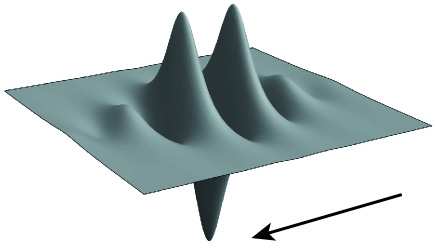
Figure 1: Sketch of a fully localised solitary wave with weak surface tension; the arrow shows the direction of wave propagation.

1.2 A variational principle

The proof of Theorem 1 is variational in nature. Fully localised solitary waves are characterised as critical points of the wave energy

$${\mathcal{E}}(\eta,\varphi)=\int_{\mathbb{R}^{2}}\left\{\frac{1}{2}\int_{0}^{1+\eta}(\varphi_{x}^{2}+\varphi_{y}^{2}+\varphi_{z}^{2})\,\mathrm{d}y+\frac{1}{2}\eta^{2}+\beta[\sqrt{1+\eta_{x}^{2}+\eta_{z}^{2}}-1]\right\}\,\mathrm{d}x\,\mathrm{d}z$$

subject to the constraint that the momentum

$${\mathcal{I}}(\eta,\varphi)=\int_{\mathbb{R}^{2}}\eta_{x}\varphi|_{y=1+\eta}\,\mathrm{d}x\,\mathrm{d}z$$

in the $x$-direction is fixed (both are conserved quantities of (1.1)–(1.4) – see articles by Zakharov & Kuznetsov [19, 20, 21, 22] and Benjamin & Olver [3]); the wave speed $c$ is the Lagrange multiplier in the variational principle $\delta({\mathcal{E}}-c{\mathcal{I}})=0$. More satisfactory representations of these functionals are obtained by means of the Dirichlet-Neumann operator $G(\eta)$ introduced by Craig [7] and defined as follows. For fixed $\Phi=\Phi(x,z)$ solve the boundary-value problem

$$\parbox{170.71652pt}{$\varphi_{xx}+\varphi_{yy}+\varphi_{zz}=0,$}0<y<1+\eta,$$

$$\parbox{170.71652pt}{$\varphi=\Phi,$}y=1+\eta,$$

$$\parbox{170.71652pt}{$\varphi_{y}=0,$}y=0$$

and define

$$G(\eta)\Phi =\sqrt{1+\eta_{x}^{2}+\eta_{z}^{2}}\left.\frac{\partial\varphi}{\partial n}\right|_{y=1+\eta}$$

$$=\varphi_{y}-\eta_{x}\varphi_{x}-\eta_{z}\varphi_{z}\Big{|}_{y=1+\eta}.$$

Working with the variables $\eta=\eta(x,z)$ and $\Phi=\Phi(x,z)$, one finds that

$${\mathcal{E}}(\eta,\Phi)=\int_{\mathbb{R}^{2}}\left\{\frac{1}{2}\Phi G(\eta)\Phi+\frac{1}{2}\eta^{2}+\beta[\sqrt{1+\eta_{x}^{2}+\eta_{z}^{2}}-1]\right\}\,\mathrm{d}x\,\mathrm{d}z,$$

$${\mathcal{I}}(\eta,\Phi)=\int_{\mathbb{R}^{2}}\eta_{x}\Phi\,\mathrm{d}x\,\mathrm{d}z.$$

We find nontrivial critical points of ${\mathcal{E}}-c{\mathcal{I}}$ in two steps. (i) For given $\eta\neq 0$, we observe that ${\mathcal{E}}(\eta,\cdot)-c{\mathcal{I}}(\eta,\cdot)$ has a unique critical point $\Phi_{\eta}$ which is the unique global minimiser $\Phi_{\eta}$ of ${\mathcal{E}}(\eta,\cdot)-c{\mathcal{I}}(\eta,\cdot)$ and satisfies $G(\eta)\Phi_{\eta}=c\eta_{x}$. (ii) We seek nontrivial critical points of the functional

$${\mathcal{J}}(\eta) :={\mathcal{E}}(\eta,\Phi_{\eta})-c{\mathcal{I}}(\eta,\Phi_{\eta})$$

$$={\mathcal{E}}(\eta,cG(\eta)^{-1}\eta_{x})-c{\mathcal{I}}(\eta,cG(\eta)^{-1}\eta_{x})$$

$$={\mathcal{K}}(\eta)-c^{2}{\mathcal{L}}(\eta),$$ (1.5)

where

$${\mathcal{K}}(\eta)=\int_{\mathbb{R}^{2}}\left(\frac{1}{2}\eta^{2}+\beta\sqrt{1+\eta_{x}^{2}+\eta_{z}^{2}}-\beta\right)\,\mathrm{d}x\,\mathrm{d}z,\qquad{\mathcal{L}}(\eta)=\frac{1}{2}\int_{\mathbb{R}^{2}}\eta\,K(\eta)\eta\,\mathrm{d}x\,\mathrm{d}z$$

and $K(\eta)=-\partial_{x}G(\eta)^{-1}\partial_{x}$. The following theorem is a reformulation of our main result in terms of critical points of ${\mathcal{J}}$.

Theorem 2.

Suppose that $0<\beta<\frac{1}{3}$ and $c^{2}=(1-\varepsilon^{2})\Lambda$. The formula (1.5) defines a smooth functional ${\mathcal{J}}_{\varepsilon}:U\rightarrow\mathbb{R}$, where $U$ is a suitably chosen open neighbourhood of the origin in $H^{3}(\mathbb{R}^{2})$, which has a nontrivial critical point for each sufficiently small value of $\varepsilon>0$.

1.3 Variational reduction

The existence of fully localised solitary waves with weak surface tension has been predicted by approximating the hydrodynamic equations (1.1)–(1.4) by simpler model equations, in particular the Davey-Stewartson equation (see Djordjevic & Redekopp [9] and Ablowitz & Segur [1]). Fully localised solitary wave solutions to the Davey-Stewartson equation have a variational characterisation, and the direct methods of the calculus of variations have been used to show that it indeed has such a solution (see Cipolatti [6] and Papanicolaou et al. [16, §5]). In this paper we seek critical points of the functional ${\mathcal{E}}-c{\mathcal{I}}$. A direct application of well-developed standard variational methods, which are optimised for semilinear partial differential equations, is not possible due to the quasilinear nature of the hydrodynamic problem (see the discussion by Groves & Sun [11] and Buffoni et al. [5]). Instead we proceed by performing a rigorous local variational reduction (akin to the variational Lyapunov-Schmidt reduction) which converts it to a perturbation of the Davey-Stewartson variational functional (Section 2). Critical points of the reduced functional are then found by applying the direct methods of the calculus of variations in a perturbative fashion (Section 3).

It is instructive to review the formal derivation of the Davey-Stewartson equation for travelling waves. We begin with the linear dispersion relation for a two-dimensional sinusoidal travelling wave train with wave number $s\geq 0$ and speed $c>0$, namely

$$c^{2}=\frac{1+\beta s^{2}}{f(s)},\qquad f(s)=s\coth s$$

(see Figure 2). For each fixed $\beta\in(0,\frac{1}{3})$ the function $s\mapsto c(s)$, $s\geq 0$ has a unique global minimum at $s=\omega>0$ (the formula $\beta=f^{\prime}(\omega)/(2\omega f(\omega)-\omega^{2}f^{\prime}(\omega))$ defines a bijection between the values of $\beta\in(0,\frac{1}{3})$ and $\omega\in(0,\infty)$); we denote the minimum value of $c^{2}$ by $\Lambda$ (so that $\Lambda=2\omega/(2\omega f(\omega)-\omega^{2}f^{\prime}(\omega))$). Note for later use that

$$g(s):=1+\beta s^{2}-\Lambda f(s)\geq 0,\qquad s\in\mathbb{R},$$ (1.6)

with equality precisely when $s=\pm\omega$. Bifurcations of nonlinear solitary waves are expected whenever the linear group and phase speeds are equal, so that $c^{\prime}(s)=0$ (see Dias & Kharif [8, §3]). We therefore expect the existence of small-amplitude solitary waves with speed near $\Lambda^{1/2}$; the waves bifurcate from a linear periodic wave train with wavenumber $\omega$.

Figure 2: Dispersion relation for a two-dimensional travelling wave train with wave number $s\geq 0$ and speed $c>0$.

Making the travelling-wave Ansatz $\eta(x,z,t)=\tilde{\eta}(x+ct,z)$ and substituting $c=\sqrt{(1-\varepsilon^{2})\Lambda}$,

$$\tilde{\eta}(x,z)=\frac{1}{2}\varepsilon\zeta(\varepsilon x,\varepsilon z)\mathrm{e}^{\mathrm{i}\omega x}+\frac{1}{2}\varepsilon\overline{\zeta(\varepsilon x,\varepsilon z)}\mathrm{e}^{-\mathrm{i}\omega x}$$ (1.7)

into equations (1.1)–(1.4), one finds that to leading order $\zeta$ satisfies the Davey-Stewartson equation

$$-a_{1}\zeta_{XX}-a_{2}\zeta_{ZZ}+a_{3}\zeta-2C_{1}{\mathcal{F}}^{-1}\left[\frac{k_{1}^{2}}{(1-\Lambda)k_{1}^{2}+k_{2}^{2}}{\mathcal{F}}[|\zeta|^{2}]\right]\zeta-2C_{2}|\zeta|^{2}\zeta=0,$$

where $X=\varepsilon x$, $Z=\varepsilon z$,

$$a_{1}=\frac{1}{8}\partial_{k_{1}}^{2}\tilde{g}(\omega,0),\qquad a_{2}=\frac{1}{8}\partial_{k_{2}}^{2}\tilde{g}(\omega,0),\qquad a_{3}=\frac{1}{4}\Lambda f(\omega),$$

$$\tilde{g}(k)=g(|k|)+\Lambda\frac{k_{2}^{2}}{|k|^{2}}f(|k|)$$

and formulae for the positive coefficients $C_{1}$, $C_{2}$ are given in Theorem 7 (see Djordjevic & Redekopp [9] and Ablowitz & Segur [1], noting the misprint in equation (2.24d)). The Davey-Stewartson equation is the Euler-Lagrange equation for the functional ${\mathcal{T}}_{0}:H^{1}(\mathbb{R}^{2})\rightarrow\mathbb{R}$ given by the formula

$${\mathcal{T}}_{0}(\zeta)=\int_{\mathbb{R}^{2}}\big{(}a_{1}|\zeta_{x}|^{2}+a_{2}|\zeta_{z}|^{2}+a_{3}|\zeta|^{2}\big{)}\,\mathrm{d}x\,\mathrm{d}z$$

$$\mbox{}-C_{1}\int_{\mathbb{R}^{2}}\frac{k_{1}^{2}}{(1-\Lambda)k_{1}^{2}+k_{2}^{2}}|{\mathcal{F}}[|\zeta|^{2}]|^{2}\,\mathrm{d}k_{1}\,\mathrm{d}k_{2}-C_{2}\int_{\mathbb{R}^{2}}|\zeta|^{4}\,\mathrm{d}x\,\mathrm{d}z,$$

where ${\mathcal{F}}$ and ${\mathcal{F}}^{-1}$ denote the Fourier and inverse Fourier transforms and we have replaced $(X,Z)$ with $(x,z)$. This functional has a nontrivial critical point (Cipolatti [6], Papanicolaou et al. [16, §5]), which of course corresponds to a fully localised solitary-wave solution of the Davey-Stewartson equation (often called a ‘lump’ solution).

Let us now return to the water-wave problem and in particular the task of finding a nontrivial critical point of the functional

$${\mathcal{J}}_{\varepsilon}(\eta)={\mathcal{K}}(\eta)-\Lambda(1-\varepsilon^{2}){\mathcal{L}}(\eta);$$

we study ${\mathcal{J}}_{\varepsilon}$ in a suitably chosen neighbourhood $U$ of the origin in its function space $H^{3}(\mathbb{R}^{2})$. The Ansatz (1.7) suggests that the spectrum of a fully localised solitary wave is concentrated near the points $(\omega,0)$ and $(-\omega,0)$. We therefore decompose $\eta$ into the sum of functions $\eta_{1}$ and $\eta_{2}$ whose Fourier transforms $\hat{\eta}_{1}$ and $\hat{\eta}_{2}$ are supported in the region $S=B_{\delta}(\omega,0)\cup B_{\delta}(-\omega,0)$ (with $\delta\in(0,\frac{\omega}{3})$) and its complement (see Figure 3), so that $\eta_{1}=\chi(D)\eta$, $\eta_{2}=(1-\chi(D))\eta$, where $\chi$ is the characteristic function of the set $S$ and $\chi(D)$ denotes the Fourier-multiplier operator with symbol $\chi$.

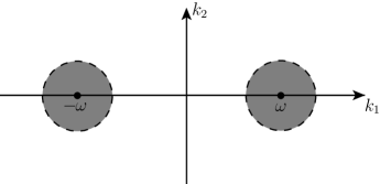
Figure 3: The support of $\hat{\eta}_{1}$ is contained in the set $S=B_{\delta}(\omega,0)\cup B_{\delta}(-\omega,0)$.

Observe that $\eta\in U$ is a critical point of ${\mathcal{J}}_{\varepsilon}$, that is

$$\mathrm{d}{\mathcal{J}}_{\varepsilon}[\eta](v)=0$$

for all $v\in{\mathcal{X}}:=H^{3}(\mathbb{R}^{2})$, if and only if

$$\mathrm{d}{\mathcal{J}}_{\varepsilon}[\eta_{1}+\eta_{2}](v_{1})=0,\qquad\mathrm{d}{\mathcal{J}}_{\varepsilon}[\eta_{1}+\eta_{2}](v_{2})=0,$$

for all $v_{1}\in{\mathcal{X}}_{1}:=\chi(D){\mathcal{X}}$ and $v_{2}\in{\mathcal{X}}_{2}:=(1-\chi(D)){\mathcal{X}}$. For sufficiently small values of $\varepsilon>0$ the second of these equations can be solved for $\eta_{2}$ as a function of $\eta_{1}$, and we thus obtain the reduced functional

$$\tilde{{\mathcal{J}}_{\varepsilon}}(\eta_{1})={\mathcal{J}}_{\varepsilon}(\eta_{1}+\eta_{2}(\eta_{1})).$$

Applying the Davey-Stewartson scaling (1.7) to $\eta_{1}$, one obtains a reduced equation for $\zeta$ which is the Euler-Lagrange equation for the functional ${\mathcal{T}}_{\varepsilon}:U_{\varepsilon}\rightarrow\mathbb{R}$ given by

$${\mathcal{T}}_{\varepsilon}(\zeta)={\mathcal{T}}_{0}(\zeta)+O(\varepsilon^{1/2}\|\zeta\|_{1}^{2})$$

(with corresponding estimates for the derivatives of the remainder term); each critical point $\zeta_{\infty}$ of ${\mathcal{T}}_{\varepsilon}$ with $\varepsilon>0$ corresponds to a critical point $\eta_{\infty}$ of $\widetilde{\mathcal{J}}_{\varepsilon}$, which in turn defines a critical point $\eta_{1}+\eta_{2}(\eta_{1})$ of ${\mathcal{J}}_{\varepsilon}$. Here $U_{\varepsilon}:=B_{R}(0)\subset H_{\varepsilon}^{1}(\mathbb{R}^{2}):=\chi(\varepsilon D)H^{1}(\mathbb{R}^{2})$, where $R$ is independent of $\varepsilon$ and can be chosen arbitrarily large.

All estimates are given in Section 2 are uniform over values of $\varepsilon$ in an interval $(0,\varepsilon_{0})$ and in general we replace $\varepsilon_{0}$ with a smaller number if necessary for the validity of our results (note in particular that $\varepsilon_{0}\rightarrow 0$ as $R\rightarrow\infty$). We consistently abbreviate inequalities of the form $g_{1}(s)\leq kg_{2}(s)$, where $k$ is a generic constant which does not depend upon $\varepsilon$, to $g_{1}(s)\lesssim g_{2}(s)$.

Remark 1.

The dispersion relation for surface waves on water of infinite depth also exhibits the features shown in Figure 2, and the corresponding travelling-wave Ansatz leads to the two-dimensional nonlinear Schrödinger equation. The dispersion relation for strong surface tension ($\beta>\frac{1}{3}$) is however qualitatively different, having a unique global minimum at $s=0$ (with $\Lambda=1$); in this case the Ansatz $\tilde{\eta}(x,z)=\varepsilon^{2}\zeta(\varepsilon x,\varepsilon^{2}z)$ leads to the KP-I equation. The two-dimensional nonlinear Schrödinger and KP-I equations have variational characterisations and ‘lump’ solutions, and the variational reduction of the water-wave problem to a perturbation of one of these equations will be discussed elsewhere.

1.4 Critical points of the reduced functional

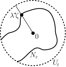
Figure 4: Any ray intersects the natural constraint manifold $N_{\varepsilon}$ in at most one point and the value of ${\mathcal{T}}_{\varepsilon}$ along such a ray attains a strict maximum at this point.

In Section 3 we seek critical points of ${\mathcal{T}}_{\varepsilon}$ by minimising it on its natural constraint set

$$N_{\varepsilon}=\{\zeta\in U_{\varepsilon}:\zeta\neq 0,\mathrm{d}{\mathcal{T}}_{\varepsilon}[\zeta](\zeta)=0\},$$

our motivation being the observation that any ground state, that is a (necessarily nontrivial) minimiser of ${\mathcal{T}}_{\varepsilon}$ over $N_{\varepsilon}$, is a critical point of ${\mathcal{T}}_{\varepsilon}$ (see Remark 7 and Willem [18, §4] for a general discussion of natural constraint sets). The natural constraint set has a geometrical interpretation (see Figure 4), namely that any ray in $B_{R}(0)\subset H_{\varepsilon}^{1}(\mathbb{R}^{2})$ intersects the natural constraint manifold $N_{\varepsilon}$ in at most one point and the value of ${\mathcal{T}}_{\varepsilon}$ along such a ray attains a strict maximum at this point. This fact is readily established by a direct calculation for $\varepsilon=0$ and deduced by a perturbation argument for $\varepsilon>0$, and similar perturbative methods yield the existence of a a minimising sequence $\{\zeta_{n}\}\subset B_{R-1}(0)$ with

$${\mathcal{T}}_{\varepsilon}|_{N_{\varepsilon}}\rightarrow\inf{\mathcal{T}}_{\varepsilon}|_{N_{\varepsilon}}>0,\qquad\mathrm{d}{\mathcal{T}}_{\varepsilon}[\zeta_{n}]\rightarrow 0$$

as $n\rightarrow\infty$.

We study minimising sequences of the above kind in Section 3.2, where the following theorem is established by a weak continuity argument.

Theorem 3.

Let $\{\zeta_{n}\}\subset B_{R-1}(0)$ be a minimising sequence for ${\mathcal{T}}_{\varepsilon}|_{N_{\varepsilon}}$ with $\mathrm{d}{\mathcal{T}}_{\varepsilon}[\zeta_{n}]\rightarrow 0$ as $n\rightarrow\infty$. There exists a sequence $\{w_{n}\}\subset\mathbb{Z}^{2}$ with the property that $\{\zeta_{n}(\cdot+w_{n})\}$ converges weakly to a nontrivial critical point $\zeta_{\infty}$ of ${\mathcal{T}}_{\varepsilon}$.

The short proof of Theorem 3 does not show that the critical point $\eta_{\infty}$ is a ground state. This deficiency is removed in Section 3.3 with the help of an abstract version of the concentration-compactness principle (Lions [14, 15]) which is given in the Appendix.

Theorem 4.

Let $\{\zeta_{n}\}\subset B_{R-1}(0)$ be a minimising sequence for ${\mathcal{T}}_{\varepsilon}|_{N_{\varepsilon}}$ with $\mathrm{d}{\mathcal{T}}_{\varepsilon}[\zeta_{n}]\rightarrow 0$ as $n\rightarrow\infty$. There exists a sequence $\{w_{n}\}\subset\mathbb{Z}^{2}$ with the property that $\{\zeta_{n}(\cdot+w_{n})\}$ converges weakly to a ground state $\zeta_{\infty}$.

We prove Theorems 3 and 4 for $\varepsilon>0$, taking advantage of the relationship between the functionals ${\mathcal{J}}_{\varepsilon}$ and ${\mathcal{T}}_{\varepsilon}$ and the fact that the spaces $\chi(\varepsilon D)H^{s}(\mathbb{R}^{2})$, $s\geq 0$ are all topologically equivalent; the function $\eta_{\infty}=\eta_{1}(\zeta_{\infty})+\eta_{2}(\eta_{1}(\zeta_{\infty}))$ given by these theorems is then a nonzero critical point of ${\mathcal{J}}_{\varepsilon}$, which concludes the proof of Theorem 1.

Note.

The main results of this paper have been announced by Buffoni [4].

2 Variational reduction

2.1 The variational functional

In this section we discuss functional-analytic aspects of the functional

$${\mathcal{J}}_{\varepsilon}(\eta)={\mathcal{K}}(\eta)-\Lambda(1-\varepsilon^{2}){\mathcal{L}}(\eta),$$

in which

$${\mathcal{K}}(\eta)=\int_{\mathbb{R}^{2}}\left(\frac{1}{2}\eta^{2}+\beta\sqrt{1+\eta_{x}^{2}+\eta_{z}^{2}}-\beta\right)\,\mathrm{d}x\,\mathrm{d}z,\qquad{\mathcal{L}}(\eta)=\frac{1}{2}\int_{\mathbb{R}^{2}}\eta\,K(\eta)\eta\,\mathrm{d}x\,\mathrm{d}z$$ (2.1)

and $K(\eta)\xi=-(\varphi|_{y=1+\eta})_{x}$, where $\varphi$ is the solution of the boundary-value problem

$$\Delta\varphi=0, 0<y<1+\eta(x,z),$$ (2.2)

$$\varphi_{y}=0, y=0,$$ (2.3)

$$\varphi_{y}-\eta_{x}\varphi_{x}-\eta_{z}\varphi_{z}=\xi_{x}, y=1+\eta(x,z)$$ (2.4)

(which is unique up to an additive constant). We examine the boundary-value problem (2.2)–(2.4) below and show in particular that the mapping $K(\cdot)\colon{\mathcal{Z}}\to{\mathcal{L}}(H^{5/2}(\mathbb{R}^{2}),H^{3/2}(\mathbb{R}^{2}))$ is analytic at the origin (Corollary 1), where

$${\mathcal{Z}}=\{\eta\in\mathcal{S}^{\prime}(\mathbb{R}^{2}):\|\eta\|_{\mathcal{Z}}:=\|\hat{\eta}_{1}\|_{L^{1}(\mathbb{R}^{2})}+\|\eta_{2}\|_{3}<\infty\},$$

$$\eta_{1}=\chi(D)\eta,\qquad\eta_{2}=(1-\chi(D))\eta,$$

and $\chi$ is the characteristic function of the set $S=B_{\delta}(\omega,0)\cup B_{\delta}(-\omega,0)$ (with $0<\delta<\frac{\omega}{3}$). In view of this result we choose $M$ sufficiently small and study ${\mathcal{J}}_{\varepsilon}$ in the set

$$U=\{\eta\in H^{3}(\mathbb{R}^{2}):\|\eta\|_{\mathcal{Z}}<M\},$$

noting that $H^{3}(\mathbb{R}^{2})$ is continuously embedded in ${\mathcal{Z}}$ and that $U$ is an open neighbourhood of the origin in $H^{3}(\mathbb{R}^{2})$. (Here, and in the remainder of the paper, we denote the usual norm for $H^{r}(\mathbb{R}^{2})$ by $\|\cdot\|_{r}$ and for $W^{m,\infty}(\mathbb{R}^{2})$ by $\|\cdot\|_{m,\infty}$.)

The boundary-value problem (2.2)–(2.4)

This boundary-value problem is studied using the change of variable

$$y^{\prime}=\frac{y}{1+\eta},\qquad u(x,y^{\prime},z)=\varphi(x,y,z),$$ (2.5)

which maps $\Sigma_{\eta}=\{(x,y,z)\colon x,z\in\mathbb{R},0<y<1+\eta(x,z)\}$ to the ‘slab’ $\Sigma=\{(x,y^{\prime},z)\colon x,z\in\mathbb{R},y^{\prime}\in(0,1)\}$. Dropping the primes, we find that the boundary-value problem is transformed into

$$\Delta u=\partial_{x}F_{1}(\eta,u)+\partial_{y}F_{3}(\eta,u)+\partial_{z}F_{2}(\eta,u), \quad 0<y<1,$$ (2.6)

$$u_{y}=0, \quad y=0,$$ (2.7)

$$u_{y}=F_{3}(\eta,u)+\xi_{x}, \quad y=1,$$ (2.8)

where

$$F_{1}(\eta,u)=-\eta u_{x}+y\eta_{x}u_{y},\quad F_{2}(\eta,u)=-\eta u_{z}+y\eta_{z}u_{y},$$

$$F_{3}(\eta,u)=\frac{\eta u_{y}}{1+\eta}+y\eta_{x}u_{x}+y\eta_{z}u_{z}-\frac{y^{2}}{1+\eta}(\eta_{x}^{2}+\eta_{z}^{2})u_{y};$$

equations (2.6)–(2.8) are studied using the following proposition, whose proof is given by Buffoni et al. [5, Propositions 2.20 and 2.21].

Proposition 1.

Suppose that $r\geq 1$. For each $F_{1}$, $F_{2}$, $F_{3}\in H^{r}(\Sigma)$ and $\xi\in H^{r+1/2}(\mathbb{R}^{2})$ the boundary-value problem

$$\Delta u=\partial_{x}F_{1}+\partial_{y}F_{3}+\partial_{z}F_{2}, \quad 0<y<1,$$

$$u_{y}=0, \quad y=0,$$

$$u_{y}=F_{3}+\xi_{x}, \quad y=1$$

admits a solution $u$ which is unique up to an additive constant. Furthermore, the mapping $(F_{1},F_{2},F_{3},\xi)\mapsto u$ defines a bounded linear operator $\Gamma:H^{r}(\Sigma)^{3}\times H^{r+1/2}(\mathbb{R}^{2})\rightarrow H^{r+1}_{\star}(\Sigma)$, where $H_{\star}^{r+1}(\Sigma)$ is the completion of

$$\mathcal{S}(\Sigma,{\mathbb{R}})=\{u\in C^{\infty}(\bar{\Sigma}):|(x,z)|^{m}|\partial_{x}^{\alpha_{1}}\partial_{y}^{\alpha_{2}}\partial_{z}^{\alpha_{3}}u|\mbox{ is bounded for all }m,\alpha_{1},\alpha_{2},\alpha_{3}\in{\mathbb{N}}_{0}\}$$

with respect to the norm

$$\|u\|_{H^{r+1}_{\star}(\Sigma)}:=\|u_{x}\|_{H^{r}(\Sigma)}+\|u_{y}\|_{H^{r}(\Sigma)}+\|u_{z}\|_{H^{r}(\Sigma)}.$$

The following result is obtained by the method used by Buffoni et al. [5, Corollary 2.23 and Proposition 2.29] (who work in the standard Sobolev space $H^{3}(\mathbb{R}^{2}))$, where the ‘elementary inequality’ quoted on page 1031 there is replaced by

$$\|\eta w\|_{H^{2}(\Sigma)} \leq\|\eta_{1}w\|_{H^{2}(\Sigma)}+\|\eta_{2}w\|_{H^{2}(\Sigma)}$$

$$\lesssim\|\eta_{1}\|_{2,\infty}\|w\|_{H^{2}(\Sigma)}+\|\eta_{2}\|_{2}\|w\|_{H^{2}(\Sigma)}$$

$$\lesssim(\|\hat{\eta}_{1}\|_{L^{1}(\mathbb{R}^{2})}+\|\eta_{2}\|_{3})\|w\|_{H^{2}(\Sigma)}$$

$$=\|\eta\|_{\mathcal{Z}}\|w\|_{H^{2}(\Sigma)}$$

(which also holds for $\|\eta_{x}w\|_{2}$ and $\|\eta_{z}w\|_{2}$ since $\hat{\eta}_{1}$ has compact support).

Lemma 1.

For each $\xi\in H^{5/2}(\mathbb{R}^{2})$ and sufficiently small $\eta\in{\mathcal{Z}}$ the boundary-value problem (2.6)–(2.8) admits a solution $u$ which is unique up to an additive constant and satisfies $u\in H^{3}_{\star}(\Sigma)$. Furthermore, the mapping ${\mathcal{Z}}\to\mathcal{L}(H^{5/2}(\mathbb{R}^{2}),H^{3}_{\star}(\Sigma))$ given by $\eta\mapsto(\xi\mapsto u)$ is analytic at the origin.

Corollary 1.

The mapping $K(\cdot)\colon{\mathcal{Z}}\to{\mathcal{L}}(H^{5/2}(\mathbb{R}^{2}),H^{3/2}(\mathbb{R}^{2}))$ is analytic at the origin.

Analyticity of the functionals and their gradients in $L^{2}(\mathbb{R}^{2})$

Corollary 2.

The formulae (2.1) define analytic functionals ${\mathcal{K}},{\mathcal{L}}:U\rightarrow\mathbb{R}$.

Our next result is proved by combining Lemma 1 with the calculation given in the proof of Lemma 2.27 in Buffoni et al. [5].

Lemma 2.

The gradients ${\mathcal{K}}^{\prime}(\eta)$ and ${\mathcal{L}}^{\prime}(\eta)$ in $L^{2}(\mathbb{R}^{2})$ exist for each $\eta\in U$ and are given by the formulae

$${\mathcal{K}}^{\prime}(\eta) =-\beta\left[\frac{\eta_{x}}{\sqrt{1+\eta_{x}^{2}+\eta_{z}^{2}}}\right]_{\!x}-\beta\left[\frac{\eta_{x}}{\sqrt{1+\eta_{x}^{2}+\eta_{z}^{2}}}\right]_{\!z}+\eta,$$

$${\mathcal{L}}^{\prime}(\eta) =-\frac{1}{2}(u_{x}^{2}+u_{z}^{2})+\frac{u_{y}^{2}}{2(1+\eta)^{2}}(\eta_{x}^{2}+\eta_{z}^{2})+\frac{u_{y}^{2}}{2(1+\eta)^{2}}-u_{x}\Bigg{|}_{y=1},$$

which define analytic functions ${\mathcal{K}}^{\prime}$, ${\mathcal{L}}^{\prime}\colon U\to H^{1}(\mathbb{R}^{2})$.

Writing

$${\mathcal{K}}(\eta)=\sum_{n=1}^{\infty}{\mathcal{K}}_{2n}(\eta),\qquad\eta\in U,$$

where ${\mathcal{K}}_{n}(\eta)=\frac{1}{n!}\mathrm{d}^{n}{\mathcal{K}}[0](\{\eta\}^{n})$ (note that ${\mathcal{K}}_{2n+1}(\eta)=0$ for each $n\in\mathbb{N}$), we obtain the explicit formulae

$${\mathcal{K}}_{2}(\eta)=\frac{1}{2}\int_{\mathbb{R}^{2}}(\eta^{2}+\beta\eta_{x}^{2}+\beta\eta_{z}^{2})\,\mathrm{d}x\,\mathrm{d}z,\qquad{\mathcal{K}}_{4}(\eta)=-\frac{\beta}{8}\int_{\mathbb{R}^{2}}\left(\eta_{x}^{2}+\eta_{z}^{2}\right)^{2}\,\mathrm{d}x\,\mathrm{d}z$$

and

$${\mathcal{K}}_{2}^{\prime}(\eta)=\eta-\beta\eta_{xx}-\beta\eta_{zz},\qquad{\mathcal{K}}_{4}^{\prime}(\eta)=\frac{\beta}{2}((\eta_{x}^{2}+\eta_{z}^{2})\eta_{x})_{x}+\frac{\beta}{2}(\eta_{x}^{2}+\eta_{z}^{2})\eta_{z})_{z}.$$

Semi-explicit formulae are also available for the leading-order terms in the corresponding series representation

$${\mathcal{L}}(\eta)=\sum_{n=2}^{\infty}{\mathcal{L}}_{n}(\eta)=\frac{1}{2}\sum_{n=2}^{\infty}\int_{\mathbb{R}^{2}}\eta K_{n}(\eta)\eta\,\mathrm{d}x\,\mathrm{d}z,\qquad\eta\in U,$$

where $K_{n}(\eta)=\frac{1}{n!}\mathrm{d}^{n}K[0](\{\eta\}^{n})$, ${\mathcal{L}}_{n}(\eta)=\frac{1}{n!}\mathrm{d}^{n}{\mathcal{L}}[0](\{\eta\}^{n})$ (see Buffoni et al. [5, Lemma 2.30 and Corollary 2.31]).

Lemma 3.

The functions ${\mathcal{L}}_{2}$, ${\mathcal{L}}_{3}$, ${\mathcal{L}}_{4}:U\rightarrow\mathbb{R}$ and ${\mathcal{L}}_{2}^{\prime}$, ${\mathcal{L}}_{3}^{\prime}$, ${\mathcal{L}}_{4}^{\prime}:U\rightarrow H^{1}(\mathbb{R}^{2})$ are given by the formulae

$${\mathcal{L}}_{2}(\eta) =\frac{1}{2}\int_{\mathbb{R}^{2}}\eta K_{0}\eta\,\mathrm{d}x\,\mathrm{d}z,$$

$${\mathcal{L}}_{3}(\eta) =\frac{1}{2}\int_{\mathbb{R}^{2}}(\eta_{x}^{2}\eta-\eta(K_{0}\eta)^{2}-\eta(L_{0}\eta)^{2})\,\mathrm{d}x\,\mathrm{d}z,$$

$${\mathcal{L}}_{4}(\eta) =\frac{1}{2}\int_{\mathbb{R}^{2}}\left(K_{0}(\eta K_{0}\eta)\,\eta K_{0}\eta+2L_{0}(\eta L_{0}\eta)\,\eta K_{0}\eta+\eta L_{0}\eta\,H_{0}(\eta L_{0}\eta)\right)\,\mathrm{d}x\,\mathrm{d}z$$

$$\qquad\mbox{}+\frac{1}{2}\int_{\mathbb{R}^{2}}\eta^{2}\left((K_{0}\eta)\eta_{xx}+(L_{0}\eta)\eta_{xz}\right)\,\mathrm{d}x\,\mathrm{d}z$$

and

$${\mathcal{L}}_{2}^{\prime}(\eta) =K_{0}\eta,$$

$${\mathcal{L}}_{3}^{\prime}(\eta) =\frac{1}{2}\left(\eta_{x}^{2}-(K_{0}\eta)^{2}-(L_{0}\eta)^{2}-2(\eta_{x}\eta)_{x}-2K_{0}(\eta K_{0}\eta)-2L_{0}(\eta L_{0}\eta)\right),$$

$$\mathcal{L}_{4}^{\prime}(\eta) =K_{0}\eta\,K_{0}(\eta K_{0}\eta)+K_{0}\eta\,L_{0}(\eta L_{0}\eta)+L_{0}\eta\,L_{0}(\eta K_{0}\eta)+L_{0}\eta\,H_{0}(\eta L_{0}\eta)$$

$$\qquad\mbox{}+\eta((K_{0}\eta)\eta_{xx}+(L_{0}\eta)\eta_{xz})+K_{2}(\eta)\eta,$$

where

$${\mathcal{F}}[K_{0}\xi]=\frac{k_{1}^{2}}{|k|^{2}}f(|k|)\hat{\xi},\quad{\mathcal{F}}[L_{0}\xi]=\frac{k_{1}k_{2}}{|k|^{2}}f(|k|)\hat{\xi},\quad{\mathcal{F}}[H_{0}\xi]=\frac{k_{2}^{2}}{|k|^{2}}f(|k|)\hat{\xi}.$$

Weak continuity of the gradients

Lemma 4.

The function ${\mathcal{K}}^{\prime}:U\rightarrow H^{1}(\mathbb{R}^{2})$ is weakly continuous.

Proof.

Because of the calculation

$$\langle{\mathcal{K}}^{\prime}(\eta),\tilde{\eta}\rangle_{1}=\langle{\mathcal{K}}^{\prime}(\eta),\tilde{\eta}\rangle_{0}-\langle{\mathcal{K}}^{\prime}(\eta),\tilde{\eta}_{xx}\rangle_{0}-\langle{\mathcal{K}}^{\prime}(\eta),\tilde{\eta}_{zz}\rangle_{0}$$

for $\eta\in U$, $\tilde{\eta}\in C_{0}^{\infty}(\mathbb{R}^{2})$ it suffices to show that ${\mathcal{K}}^{\prime}$ is a weakly continuous function $U\rightarrow L^{2}(\mathbb{R}^{2})$.

Suppose that $\{\eta_{n}\}\subset U$ converges weakly in $H^{3}(\mathbb{R}^{2})$ to $\eta_{\infty}\in U$, so that $\{\eta_{n}\}$, $\{\eta_{nx}\}$, $\{\eta_{nz}\}$ converge strongly in $C_{\mathrm{loc}}(\mathbb{R}^{2})$ to $\eta_{\infty}$, $\eta_{\infty x}$, $\eta_{\infty z}$. Using the formula

$$\langle{\mathcal{K}}^{\prime}(\eta),\tilde{\eta}\rangle_{0}=\int_{\mathbb{R}^{2}}\left(\frac{\beta\eta_{x}\tilde{\eta}_{x}}{\sqrt{1+\eta_{x}^{2}+\eta_{z}^{2}}}+\frac{\beta\eta_{z}\tilde{\eta}_{z}}{\sqrt{1+\eta_{x}^{2}+\eta_{z}^{2}}}+\eta\tilde{\eta}\right)\,\mathrm{d}x\,\mathrm{d}z,$$

we conclude that $\langle{\mathcal{K}}^{\prime}(\eta_{n}),\tilde{\eta}\rangle_{0}\rightarrow\langle{\mathcal{K}}^{\prime}(\eta_{\infty}),\tilde{\eta}\rangle_{0}$ for each $\tilde{\eta}\in C_{0}^{\infty}(\mathbb{R}^{2})$. ∎

To obtain the corresponding result for ${\mathcal{L}}^{\prime}$ we first establish some further mapping properties of the operator $K(\cdot)\colon U\to{\mathcal{L}}(H^{5/2}(\mathbb{R}^{2}),H^{3/2}(\mathbb{R}^{2}))$. For this purpose we note that the solution of the boundary-value problem (2.6)–(2.8) (with $\eta\in U$, $\xi\in H^{5/2}(\mathbb{R}^{2})$) can be characterised as the unique solution of the equation

$$u=\Gamma(F_{1}(\eta,u),F_{2}(\eta,u),F_{3}(\eta,u),\xi)$$

(see Proposition 1).

Proposition 2.

Suppose that $\{\eta_{n}\}\subset U$ converges weakly in $H^{3}(\mathbb{R}^{2})$ to $\eta_{\infty}\in U$ and $\{\xi_{n}\}\subset H^{5/2}(\mathbb{R}^{2})$ converges weakly in $H^{5/2}(\mathbb{R}^{2})$ to $\xi_{\infty}$.

• The sequence $\{K(\eta_{n})\xi_{n}\}$ converges weakly in $H^{3/2}(\mathbb{R}^{2})$ to $K(\eta_{\infty})\xi_{\infty}$.

• The sequence $\{(K(\eta_{\infty})-K(0))\xi_{n}\}$ converges strongly in $H^{1/2}(\mathbb{R}^{2})$ to $(K(\eta_{\infty})-K(0))\xi_{\infty}$.

• For each $\rho\in H^{3}(\mathbb{R}^{2})$ the sequence $\left\{\big{(}\mathrm{d}K[\eta_{n}](\rho)\big{)}\xi_{n}\right\}$ converges strongly in $H^{1/2}(\mathbb{R}^{2})$ to $\big{(}\mathrm{d}K[\eta_{\infty}](\rho)\big{)}\xi_{\infty}$.

Proof.

(i) Let $u_{n}$ and $u_{\infty}$ be the solutions to (2.6)–(2.8) with $\eta$, $\xi$ replaced by respectively $\eta_{n}$, $\xi_{n}$ and $\eta_{\infty}$, $\xi_{\infty}$, so that

$$u_{n}=\Gamma(F_{1}(\eta_{n},u_{n}),F_{2}(\eta_{n},u_{n}),F_{3}(\eta_{n},u_{n}),\xi_{n})$$

and

$$u_{\infty}=\Gamma(F_{1}(\eta_{\infty},u_{\infty}),F_{2}(\eta_{\infty},u_{\infty}),F_{3}(\eta_{\infty},u_{\infty}),\xi_{\infty}).$$

Since $\{\eta_{n}\}$ and $\{\xi_{n}\}$ are bounded in respectively $H^{3}(\mathbb{R}^{2})$ and $H^{5/2}(\mathbb{R}^{2})$, it follows from Lemma 1 that $\{u_{n}\}$ is bounded in $H^{3}_{\star}(\Sigma)$. The following argument shows that any weakly convergent subsequence of $\{u_{n}\}$ has weak limit $u_{\infty}$, so that $\{u_{n}\}$ itself converges weakly to $u_{\infty}$; in particular $K(\eta_{n})\xi_{n}=-u_{nx}(x,1,z)\rightharpoonup-u_{\infty x}(x,1,z)=K(\eta_{\infty})\xi_{\infty}$ in $H^{3/2}(\mathbb{R}^{2})$.

Suppose that (a subsequence of) $\{u_{n}\}$ converges weakly to $u_{0}$ in $H^{3}_{\star}(\Sigma)$. Observing that $\{\eta_{n}\}$ converges strongly in $H^{2}_{\mathrm{loc}}(\mathbb{R}^{2})$ to $\eta_{\infty}$, $\{u_{n}\}$ converges strongly in $H^{2}_{\star,\mathrm{loc}}(\Sigma)$ to $u_{0}$ and hence $\{F_{j}(\eta_{n},u_{n})\}$ converges strongly in $H^{1}_{\mathrm{loc}}(\Sigma)$ to $F_{j}(\eta_{\infty},u_{0})$, $j=1,2,3$, we find that $u_{0}$ is the solution to (2.6)–(2.8) with $\eta$ and $\xi$ replaced by respectively $\eta_{\infty}$ and $\xi_{\infty}$, so that $u_{0}=u_{\infty}$.

(ii) Define

$$v_{n}=\Gamma(F_{1}(\eta_{\infty},u_{n}),F_{2}(\eta_{\infty},u_{n}),F_{3}(\eta_{\infty},u_{n}),0)$$

and repeat the argument used in part (i): the sequence $\{v_{n}\}$ converges weakly in $H^{3}_{\star}(\Sigma)$ to $v_{\infty}$, and

$$v_{\infty}=\Gamma(F_{1}(\eta_{\infty},u_{\infty}),F_{2}(\eta_{\infty},u_{\infty}),F_{3}(\eta_{\infty},u_{\infty}),0).$$

Furthermore $\{F_{j}(\eta_{\infty},u_{n})\}$ converges strongly to $F_{j}(\eta_{\infty},u_{\infty})$ in $H^{1}(\Sigma)$ since

$$\|F_{j}(\eta_{\infty},u_{n}-u_{\infty})\|_{1} \leq\|F_{j}(\eta_{\infty},u_{n}-u_{\infty})\|_{H^{1}(|(x,z)|<R)}+\|F_{j}(\eta_{\infty},u_{n}-u_{\infty})\|_{H^{1}(|(x,z)|>R)}$$

$$\lesssim\|F_{j}(\eta_{\infty},u_{n}-u_{\infty})\|_{H^{1}(|(x,z)|<R)}+\|\eta_{\infty}\|_{H^{3}(|(x,z)|>R)}$$

$$\rightarrow 0$$

as $n\rightarrow\infty$ (note that $\|\eta_{\infty}\|_{H^{3}(|(x,z)|>R)}\rightarrow 0$ as $R\rightarrow\infty$ and $\{F_{j}(\eta_{\infty},u_{n})\}$ converges strongly in $H^{1}(|(x,z)|<R)$ to $F_{j}(\eta_{\infty},u_{\infty})$). It follows that $\{v_{n}\}$ converges strongly in $H_{\star}^{2}(\Sigma)$ to $v_{\infty}$ and $(K(\eta_{\infty})-K(0))\xi_{n}=-v_{nx}(x,1,z)\rightarrow-v_{\infty x}(x,1,z)=(K(\eta_{\infty})-K(0))\xi_{\infty}$ in $H^{1/2}(\mathbb{R}^{2})$.

(iii) Let $w_{n}=\mathrm{d}_{1}u_{n}[\eta_{n},\xi_{n}](\rho)$, so that

$$w_{n} =\Gamma(F_{1}(\eta_{n},w_{n}),F_{2}(\eta_{n},w_{n}),F_{3}(\eta_{n},w_{n}),0)$$

$$\qquad\mbox{}+\Gamma(\mathrm{d}_{1}F_{1}[\eta_{n},u_{n}](\rho),\mathrm{d}_{1}F_{2}[\eta_{n},u_{n}](\rho),\mathrm{d}_{1}F_{3}[\eta_{n},u_{n}](\rho),0),$$ (2.9)

where

$$\mathrm{d}_{1}F_{1}[\eta,u](\rho) =-\rho u_{x}+y\rho_{x}u_{y},$$

$$\mathrm{d}_{1}F_{2}[\eta,u](\rho) =-\rho u_{z}+y\rho_{z}u_{y},$$

$$\mathrm{d}_{1}F_{3}[\eta,u](\rho) =\frac{\rho u_{y}}{1+\eta}-\frac{\eta u_{y}\rho}{(1+\eta)^{2}}+y\rho_{x}u_{x}+y\rho_{z}u_{z}$$

$$\qquad\mbox{}+\frac{y^{2}\rho}{(1+\eta)^{2}}(\eta_{x}^{2}+\eta_{z}^{2})u_{y}-\frac{2y^{2}}{1+\eta}(\eta_{x}\rho_{x}+\eta_{z}\rho_{z})u_{y};$$

the usual argument shows that $\{w_{n}\}$ converges weakly in $H^{3}_{\star}(\Sigma)$ to $w_{\infty}$ and that$w_{\infty}=\mathrm{d}_{1}u_{\infty}[\eta_{\infty},\xi_{\infty}](\rho)$.

The argument used in part (ii) shows that $\{\mathrm{d}_{1}F_{j}[\eta_{n},u_{n}](\rho)\}$ converges strongly in $H^{1}_{\star}(\Sigma)$ to $\mathrm{d}_{1}F_{j}[\eta_{\infty},u_{\infty}](\rho)$, so that $\{c_{n}\}$ with $c_{n}=\Gamma(\mathrm{d}_{1}F_{1}[\eta_{n},u_{n}](\rho),\mathrm{d}_{1}F_{2}[\eta_{n},u_{n}](\rho),\mathrm{d}_{1}F_{3}[\eta_{n},u_{n}](\rho),0)$ is strongly convergent in $H_{\star}^{2}(\Sigma)$. Define $A(\eta)\in{\mathcal{L}}(H_{\star}^{2}(\Sigma))$ by the formula $A(\eta)=\linebreak\Gamma(F_{1}(\eta,\cdot),F_{2}(\eta,\cdot),F_{3}(\eta,\cdot),0)$, choosing $M$ small enough so that $\sup_{\eta\in U}\|A(\eta)\|<1$, and observe that $A_{n}=A(\eta_{n})$ has the property that $\{A_{n}b_{n}\}$ is strongly convergent whenever $\{b_{n}\}$ is strongly convergent. Writing (2.9) in the abstract form

$$w_{n}=A_{n}w_{n}+c_{n},$$

we find from a familiar Neumann-series argument that $\{w_{n}\}$ is a Cauchy sequence in $H^{2}_{\star}(\Sigma)$ which therefore converges strongly to its weak limit $w_{\infty}$. It follows that $\big{(}\mathrm{d}K[\eta_{n}](\rho)\big{)}\xi_{n}=-w_{nx}(x,1,z)\rightarrow-w_{\infty x}(x,1,z)=\big{(}\mathrm{d}K[\eta_{\infty}](\rho)\big{)}\xi_{\infty}$ in $H^{1/2}(\mathbb{R}^{2})$. ∎

Lemma 5.

The function ${\mathcal{L}}^{\prime}:U\rightarrow H^{1}(\mathbb{R}^{2})$ is weakly continuous.

Proof.

It suffices to show that ${\mathcal{L}}^{\prime}$ is a weakly continuous function $U\rightarrow L^{2}(\mathbb{R}^{2})$. Suppose that $\{\eta_{n}\}\subset U$ converges weakly in $H^{3}(\mathbb{R}^{2})$ to $\eta_{\infty}\in U$. Using the formula

$$\langle{\mathcal{L}}^{\prime}(\eta),\rho\rangle_{0}=\langle K(\eta)\eta,\rho\rangle_{0}+\frac{1}{2}\int_{\mathbb{R}^{2}}\eta\big{(}\mathrm{d}K[\eta](\rho)\big{)}\eta\,\mathrm{d}x\,\mathrm{d}z$$

and Proposition 2, we find that $\langle{\mathcal{L}}^{\prime}(\eta_{n}),\rho\rangle_{0}\rightarrow\langle{\mathcal{L}}^{\prime}(\eta_{\infty}),\rho\rangle_{0}$ for each $\rho\in C_{0}^{\infty}(\mathbb{R}^{2})$. ∎

Corollary 3.

The function ${\mathcal{J}}_{\varepsilon}^{\prime}:U\rightarrow H^{1}(\mathbb{R}^{2})$ is weakly continuous.

Remark 2.

The functions ${\mathcal{L}}_{3}^{\prime}$, ${\mathcal{L}}_{4}^{\prime}$ and ${\mathcal{K}}_{4}^{\prime}:U\rightarrow H^{1}(\mathbb{R}^{2})$ are also weakly continuous.

Suppose that $\{\eta_{n}\}\subset U$ converges weakly in $H^{3}(\mathbb{R}^{2})$ to $\eta_{\infty}\in U$. It follows that $\{K_{0}\eta_{n}\}$, $\{L_{0}\eta_{n}\}$ converge strongly in $L^{4}_{\mathrm{loc}}(\mathbb{R}^{2})$ to $K_{0}\eta_{\infty}$, $L_{0}\eta_{\infty}$ and $\{\eta_{n}K_{0}\eta_{n}\}$, $\{\eta_{n}L_{0}\eta_{n}\}$, $\{(K_{0}\eta_{n})^{2}\}$, $\{(L_{0}\eta_{n})^{2}\}$, $\{\eta_{nx}^{2}\}$ converge strongly in $L^{2}_{\mathrm{loc}}(\mathbb{R}^{2})$ to $\eta_{\infty}K_{0}\eta_{\infty}$, $\eta_{\infty}L_{0}\eta_{\infty}$, $(K_{0}\eta_{\infty})^{2}$, $(L_{0}\eta_{\infty})^{2}$, $\eta_{\infty x}^{2}$. Examining the expression for ${\mathcal{L}}_{3}^{\prime}(\eta)$ given in Lemma 3, we conclude that $\langle{\mathcal{L}}_{3}^{\prime}(\eta_{n}),\tilde{\eta}\rangle_{0}$ converges to $\langle{\mathcal{L}}_{3}^{\prime}(\eta_{\infty}),\tilde{\eta}\rangle_{0}$ for each $\tilde{\eta}\in C_{0}^{\infty}(\mathbb{R}^{2})$.

Similar arguments show that $\langle{\mathcal{K}}_{4}^{\prime}(\eta_{n}),\tilde{\eta}\rangle_{0}\rightarrow\langle{\mathcal{K}}_{4}^{\prime}(\eta),\tilde{\eta}\rangle_{0}$ and $\langle{\mathcal{L}}_{4}^{\prime}(\eta_{n}),\tilde{\eta}\rangle_{0}\rightarrow\langle{\mathcal{L}}_{4}^{\prime}(\eta),\tilde{\eta}\rangle_{0}$ as $n\rightarrow\infty$ for each $\tilde{\eta}\in C_{0}^{\infty}(\mathbb{R}^{2})$.

Further notation

Finally, we denote the superquadratic part of ${\mathcal{J}}_{\varepsilon}(\eta)$ by ${\mathcal{N}}(\eta)$, that is write

$${\mathcal{N}}(\eta):= \,{\mathcal{J}}_{\varepsilon}(\eta)-({\mathcal{K}}_{2}(\eta)-\Lambda(1-\varepsilon^{2}){\mathcal{L}}_{2}(\eta))$$

$$= \,{\mathcal{K}}_{\mathrm{nl}}(\eta)-\Lambda(1-\varepsilon^{2}){\mathcal{L}}_{\mathrm{nl}}(\eta),$$

where

$${\mathcal{K}}_{\mathrm{nl}}(\eta)=\sum_{n=2}^{\infty}{\mathcal{K}}_{2n}(\eta),\qquad{\mathcal{L}}_{\mathrm{nl}}(\eta)=\sum_{n=3}^{\infty}{\mathcal{L}}_{n}(\eta);$$

in view of the above calculations we also use the notation

$${\mathcal{K}}_{\mathrm{r}}(\eta):={\mathcal{K}}_{\mathrm{nl}}(\eta)-{\mathcal{K}}_{4}(\eta),\qquad{\mathcal{L}}_{\mathrm{r}}(\eta):={\mathcal{L}}_{\mathrm{nl}}(\eta)-{\mathcal{L}}_{3}(\eta)-{\mathcal{L}}_{4}(\eta).$$

Note that ${\mathcal{N}}$, ${\mathcal{K}}_{\mathrm{nl}}$, ${\mathcal{L}}_{\mathrm{nl}}$, ${\mathcal{K}}_{\mathrm{r}}$ and ${\mathcal{L}}_{\mathrm{r}}:U\rightarrow H^{1}(\mathbb{R}^{2})$ are also weakly continuous.

2.2 The reduction procedure

The next step is to decompose ${\mathcal{X}}=H^{3}(\mathbb{R}^{2})$ into the direct sum of the weakly closed subspaces ${\mathcal{X}}_{1}=\chi(D){\mathcal{X}}$ and ${\mathcal{X}}_{2}=(1-\chi(D)){\mathcal{X}}$. Observe that $\eta\in U$ is a critical point of ${\mathcal{J}}_{\varepsilon}$, that is

$$\mathrm{d}{\mathcal{J}}_{\varepsilon}[\eta](\rho)=0$$

for all $\rho\in{\mathcal{X}}$, if and only if

$$\mathrm{d}{\mathcal{J}}_{\varepsilon}[\eta_{1}+\eta_{2}](\rho_{1})=0,\qquad\mathrm{d}{\mathcal{J}}_{\varepsilon}[\eta_{1}+\eta_{2}](\rho_{2})=0,$$

or equivalently

$$\langle{\mathcal{J}}_{\varepsilon}^{\prime}(\eta_{1}+\eta_{2}),\rho_{1}\rangle_{0}=0,\qquad\langle{\mathcal{J}}_{\varepsilon}^{\prime}(\eta_{1}+\eta_{2}),\rho_{2}\rangle_{0}=0,$$ (2.10)

for all $\rho_{1}\in{\mathcal{X}}_{1}$ and $\rho_{2}\in{\mathcal{X}}_{2}$. Equations (2.10) are given explicitly by

$$\eta_{1}-\beta\eta_{1xx}-\beta\eta_{1zz}-\Lambda K_{0}\eta_{1}+\varepsilon^{2}\Lambda K_{0}\eta_{1}\hskip 130.08621pt$$

$$\mbox{}+\chi(D)\left({\mathcal{N}}^{\prime}(\eta_{1}+\eta_{2})+\Lambda(1-\varepsilon^{2}){\mathcal{L}}_{3}^{\prime}(\eta_{1})\right) =0,$$ (2.11)

$$\underbrace{\eta_{2}-\beta\eta_{2xx}-\beta\eta_{2zz}-\Lambda K_{0}\eta_{2}}_{\displaystyle=\tilde{g}(D)\eta_{2}}+\varepsilon^{2}\Lambda K_{0}\eta_{2}+(1-\chi(D)){\mathcal{N}}^{\prime}(\eta_{1}+\eta_{2}) =0,$$ (2.12)

where

$$\tilde{g}(k):=g(|k|)+\Lambda\frac{k_{2}^{2}}{|k|^{2}}f(|k|)\geq 0$$

with equality if and only if $k=\pm(\omega,0)$ (see the comments to equation (1.6)) and we have used the fact that $\chi(D){\mathcal{L}}_{3}^{\prime}(\eta_{1})$ vanishes (so that the nonlinear term in (2.11) is at leading order cubic in $\eta_{1}$). We accordingly write

$$\eta_{2}=F(\eta_{1})+\eta_{3},\qquad F(\eta_{1}):=\Lambda(1-\varepsilon^{2}){\mathcal{F}}^{-1}\left[\frac{1-\chi(k)}{\tilde{g}(k)}{\mathcal{F}}[{\mathcal{L}}_{3}^{\prime}(\eta_{1})]\right]$$

and (2.12) in the form

$$\eta_{3}=-{\mathcal{F}}^{-1}\left[\frac{1-\chi(k)}{\tilde{g}(k)}{\mathcal{F}}\left[\Lambda(1-\varepsilon^{2}){\mathcal{L}}_{3}^{\prime}(\eta_{1})+{\mathcal{N}}^{\prime}(\eta_{1}+F(\eta_{1})+\eta_{3})+\Lambda\varepsilon^{2}K_{0}(F(\eta_{1})+\eta_{3})\right]\right]$$ (2.13)

(with the requirement that $\eta_{1}+F(\eta_{1})+\eta_{3}\in U$).

Proposition 3.

The mapping

$$f\mapsto{\mathcal{F}}^{-1}\left[\frac{1-\chi(k)}{\tilde{g}(k)}\hat{f}\right]$$

defines a bounded linear operator $H^{1}(\mathbb{R}^{2})\to H^{3}(\mathbb{R}^{2})$.

We proceed by solving (2.13) for $\eta_{3}$ as a function of $\eta_{1}$ using the following fixed-point theorem, which is a straightforward extension of a standard result in nonlinear analysis.

Theorem 5.

Let ${\mathcal{Y}}_{1}$, ${\mathcal{Y}}_{2}$ be Banach spaces, $Y_{1}$, $Y_{2}$ be closed sets in, respectively, ${\mathcal{Y}}_{1}$, ${\mathcal{Y}}_{2}$ containing the origin and $G\colon Y_{1}\times Y_{2}\to{\mathcal{Y}}_{2}$ be a smooth function. Suppose that there exists a continuous function $r\colon Y_{1}\to[0,\infty)$ such that

$$\|G(y_{1},0)\|\leq\frac{r}{2},\quad\|\mathrm{d}_{2}G[y_{1},y_{2}]\|\leq\frac{1}{3}$$

for each $y_{2}\in\bar{B}_{r}(0)\subset Y_{2}$ and each $y_{1}\in Y_{1}$.

Under these hypotheses there exists for each $y_{1}\in Y_{1}$ a unique solution $y_{2}=y_{2}(y_{1})$ of the fixed-point equation

$$y_{2}=G(y_{1},y_{2})$$

satisfying $y_{2}(y_{1})\in\bar{B}_{r}(0)$. Moreover $y_{2}(y_{1})$ is a smooth function of $y_{1}\in Y_{1}$ and in particular satisfies the estimate

$$\|\mathrm{d}y_{2}[y_{1}]\|\leq 2\|\mathrm{d}_{1}G[y_{1},y_{2}(y_{1})]\|$$

for its first derivative and the estimate

$$\|\mathrm{d}^{2}y_{2}[y_{1}] \|\leq 2\|\mathrm{d}_{1}^{2}G[y_{1},y_{2}(y_{1})]\|$$

$$\qquad\mbox{}+8\|\mathrm{d}_{1}\mathrm{d}_{2}G[y_{1},y_{2}(y_{1})]\|\|\mathrm{d}_{1}G[y_{1},y_{2}(y_{1})]\|+8\|\mathrm{d}_{2}^{2}G[y_{1},y_{2}(y_{1})]\|\|\mathrm{d}_{1}G[y_{1},y_{2}(y_{1})]\|^{2}$$

for its second derivative.

We apply Theorem 5 to equation (2.13) with ${\mathcal{Y}}_{1}={\mathcal{X}}_{1}$, ${\mathcal{Y}}_{2}={\mathcal{X}}_{2}$, equipping ${\mathcal{X}}_{1}$ with the scaled norm

$$|{\mskip-2.0mu}|{\mskip-2.0mu}|\eta|{\mskip-2.0mu}|{\mskip-2.0mu}|:=\left(\int_{\mathbb{R}^{2}}(1+\varepsilon^{-2}((|k_{1}|-\omega)^{2}+k_{2}^{2}))|\hat{\eta}(k)|^{2}\,\mathrm{d}k_{1}\,\mathrm{d}k_{2}\right)^{\!1/2}$$

and ${\mathcal{X}}_{2}$ with the usual norm for $H^{3}(\mathbb{R}^{2})$, and taking $Y_{1}=X_{1}$, $Y_{2}=X_{3}$, where

$$X_{1}=\{\eta_{1}\in{\mathcal{X}}_{1}\colon|{\mskip-2.0mu}|{\mskip-2.0mu}|\eta_{1}|{\mskip-2.0mu}|{\mskip-2.0mu}|\leq R_{1}\},\qquad X_{3}=\{\eta_{3}\in{\mathcal{X}}_{2}\colon\|\eta_{3}\|_{3}\leq R_{3}\};$$

the function $G$ is given by the right-hand side of (2.13). The following proposition shows that

$$\|\hat{\eta}_{1}\|_{L^{1}(\mathbb{R}^{2})}\lesssim\varepsilon^{\theta}|{\mskip-2.0mu}|{\mskip-2.0mu}|\eta_{1}|{\mskip-2.0mu}|{\mskip-2.0mu}|,\qquad\eta_{1}\in{\mathcal{X}}_{1},$$ (2.14)

for each fixed $\theta\in(0,1)$, so that we can guarantee that $\|\hat{\eta}_{1}\|_{L^{1}(\mathbb{R}^{2})}<M/2$ for all $\eta_{1}\in X_{1}$ for an arbitrarily large value of $R_{1}$; the value of $R_{3}$ is then constrained by the requirement that $\|F(\eta_{1})+\eta_{3}\|_{3}<M/2$ for all $\eta_{1}\in X_{1}$ and $\eta_{3}\in X_{3}$, so that $\eta_{1}+F(\eta_{1})+\eta_{3}\in U=B_{M}(0)$ (Corollary 4 below asserts that $\|F(\eta_{1})\|_{3}=O(\varepsilon^{\theta})$ uniformly over $\eta_{1}\in X_{1}$).

Proposition 4.

The estimate

$$\|\hat{\eta}_{1}\|_{L^{1}(\mathbb{R}^{2})}\lesssim\varepsilon|\!\log\varepsilon||{\mskip-2.0mu}|{\mskip-2.0mu}|\eta_{1}|{\mskip-2.0mu}|{\mskip-2.0mu}|$$

holds for each $\eta_{1}\in{\mathcal{X}}_{1}$.

Proof.

Observe that

$$\int_{\mathbb{R}^{2}}|\hat{\eta}_{1}(k)|\,\mathrm{d}k_{1}\,\mathrm{d}k_{2} =\int_{\mathbb{R}^{2}}\frac{(1+\varepsilon^{-2}((|k_{1}|-\omega)^{2}+k_{2}^{2}))^{1/2}}{(1+\varepsilon^{-2}((|k_{1}|-\omega)^{2}+k_{2}^{2}))^{1/2}}|\hat{\eta}_{1}(k)|\,\mathrm{d}k_{1}\,\mathrm{d}k_{2}$$

$$\leq 2|{\mskip-2.0mu}|{\mskip-2.0mu}|\eta|{\mskip-2.0mu}|{\mskip-2.0mu}|\left(\int_{B_{\delta}(\omega,0)}\frac{1}{1+\varepsilon^{-2}((k_{1}-\omega)^{2}+k_{2}^{2})}\,\mathrm{d}k_{1}\,\mathrm{d}k_{2}\right)^{1/2},$$

$$=2\varepsilon|{\mskip-2.0mu}|{\mskip-2.0mu}|\eta|{\mskip-2.0mu}|{\mskip-2.0mu}|\left(\int_{|k|<\delta/\varepsilon}\frac{1}{1+|k|^{2}}\,\mathrm{d}k_{1}\,\mathrm{d}k_{2}\right)^{1/2}$$

$$=2\sqrt{\pi}\varepsilon(\log(1+\delta^{2}\varepsilon^{-2}))^{1/2}|{\mskip-2.0mu}|{\mskip-2.0mu}|\eta|{\mskip-2.0mu}|{\mskip-2.0mu}|.\qed$$

We proceed by systematically estimating each term appearing in the equation for $G$, writing

$$\Lambda(1-\varepsilon^{2}){\mathcal{L}}_{3}^{\prime}(\eta_{1})+{\mathcal{N}}^{\prime}(\eta)\\ ={\mathcal{K}}_{\mathrm{nl}}^{\prime}(\eta_{1}+F(\eta_{1})+\eta_{3})-\Lambda(1-\varepsilon^{2})\big{(}{\mathcal{L}}_{3}^{\prime}(\eta)-{\mathcal{L}}_{3}^{\prime}(\eta_{1})+{\mathcal{L}}_{4}^{\prime}(\eta)+{\mathcal{L}}_{\mathrm{r}}^{\prime}(\eta)\big{)},$$

where $\eta=\eta_{1}+F(\eta_{1})+\eta_{3}$, and using the inequalities (2.14) and

$$\|\eta_{1}\|_{3}\lesssim|{\mskip-2.0mu}|{\mskip-2.0mu}|\eta_{1}|{\mskip-2.0mu}|{\mskip-2.0mu}|$$

to handle $\eta_{1}$; note in particular that

$$\|\eta\|_{\mathcal{Z}}\lesssim\varepsilon^{\theta}|{\mskip-2.0mu}|{\mskip-2.0mu}|\eta_{1}|{\mskip-2.0mu}|{\mskip-2.0mu}|+\|\eta_{3}\|_{3},\qquad\|\eta\|_{3}\lesssim|{\mskip-2.0mu}|{\mskip-2.0mu}|\eta_{1}|{\mskip-2.0mu}|{\mskip-2.0mu}|+\|\eta_{3}\|_{3}$$

for each $\eta\in H^{3}(\mathbb{R}^{2})$.

In order to estimate $F(\eta_{1})$ we write ${\mathcal{L}}_{3}^{\prime}(\eta)=m(\{\eta\}^{2})$, where

$$m(u,v) =\frac{1}{2}\left(u_{x}v_{x}-(K_{0}u)(K_{0}v)-(L_{0}u)(L_{0}v)\right)$$

$$\qquad\mbox{}+\frac{1}{2}\left(-(u_{x}v+uv_{x})_{x}-K_{0}(uK_{0}v+vK_{0}u)-L_{0}(uL_{0}v+vL_{0}u)\right)$$

(see Lemma 3), and note that

$$\mathrm{d}{\mathcal{L}}_{3}^{\prime}[\eta](v)=2m(\eta,v),\qquad\mathrm{d^{2}}{\mathcal{L}}_{3}^{\prime}[\eta](v,w)=2m(v,w).$$

Proposition 5.

The estimate

$$\|m(u,v)\|_{1}\lesssim\|u\|_{\mathcal{Z}}\|v\|_{3},$$

holds for each $u$, $v\in H^{3}(\mathbb{R}^{2})$.

Proof.

We estimate

$$\|m(u,v)\|_{1} \lesssim(\|u_{1}\|_{3,\infty}+\|K_{0}u_{1}\|_{2,\infty}+\|L_{0}u_{1}\|_{2,\infty}+\|u_{2}\|_{3})\|v\|_{3}$$

$$\lesssim(\|\hat{u}_{1}\|_{L^{1}(\mathbb{R}^{2})}+\|u_{2}\|_{3})\|v\|_{3}$$

$$=\|u\|_{\mathcal{Z}}\|v\|_{3},$$

where the second line follows from the fact that

$$\|u_{1}\|_{m,\infty},\ \|K_{0}u_{1}\|_{m,\infty},\ \|L_{0}u_{1}\|_{m,\infty},\|H_{0}u_{1}\|_{m,\infty}\lesssim\|\hat{u}_{1}\|_{L_{1}(\mathbb{R}^{2})}$$

for each $m\in{\mathbb{N}}_{0}$ (since $\hat{u}_{1}$ has compact support). ∎

Corollary 4.

The estimates

$$\|F(\eta_{1})\|_{3}\lesssim\varepsilon^{\theta}|{\mskip-2.0mu}|{\mskip-2.0mu}|\eta_{1}|{\mskip-2.0mu}|{\mskip-2.0mu}|^{2},\quad\|\mathrm{d}F[\eta_{1}]\|_{{\mathcal{L}}({\mathcal{X}}_{1},{\mathcal{X}}_{2})}\lesssim\varepsilon^{\theta}|{\mskip-2.0mu}|{\mskip-2.0mu}|\eta_{1}|{\mskip-2.0mu}|{\mskip-2.0mu}|,\quad\|\mathrm{d}^{2}F[\eta_{1}]\|_{{\mathcal{L}}^{2}({\mathcal{X}}_{1},{\mathcal{X}}_{2})}\lesssim\varepsilon^{\theta}$$

hold for each $\eta_{1}\in X_{1}$, where ${\mathcal{L}}({\mathcal{X}}_{1},{\mathcal{X}}_{2})$ and ${\mathcal{L}}^{2}({\mathcal{X}}_{1},{\mathcal{X}}_{2})$ denote the spaces of bounded linear and bilinear operators ${\mathcal{X}}_{1}\rightarrow{\mathcal{X}}_{2}$.

Remark 3.

Noting that

$$K_{0}F(\eta_{1})=\Lambda(1-\varepsilon^{2}){\mathcal{F}}^{-1}\left[\frac{1-\chi(k)}{\tilde{g}(k)}\frac{k_{1}^{2}}{|k|^{2}}f(|k|){\mathcal{L}}_{3}^{\prime}(\eta_{1})\right]$$

and that ${\mathcal{L}}_{3}^{\prime}(\eta_{1})$ has compact support, one finds that $K_{0}F(\eta_{1})$ satisfies the same estimates as $F(\eta_{1})$.

The quantity

$${\mathcal{A}}(\eta_{1},\eta_{3}): ={\mathcal{L}}_{3}^{\prime}(\eta_{1}+F(\eta_{1})+\eta_{3})-{\mathcal{L}}_{3}^{\prime}(\eta_{1})$$

$$=2m(\eta_{1},F(\eta_{1})+\eta_{3})+m(F(\eta_{1})+\eta_{3},F(\eta_{1})+\eta_{3})$$

is estimated by combining Proposition 5 and Corollary 4 using the chain rule.

Lemma 6.

The estimates

• $\|{\mathcal{A}}(\eta_{1},\eta_{3})\|_{1}\lesssim\varepsilon^{2\theta}|{\mskip-2.0mu}|{\mskip-2.0mu}|\eta_{1}|{\mskip-2.0mu}|{\mskip-2.0mu}|^{3}+\varepsilon^{\theta}|{\mskip-2.0mu}|{\mskip-2.0mu}|\eta_{1}|{\mskip-2.0mu}|{\mskip-2.0mu}|^{2}\|\eta_{3}\|_{3}+\varepsilon^{\theta}|{\mskip-2.0mu}|{\mskip-2.0mu}|\eta_{1}|{\mskip-2.0mu}|{\mskip-2.0mu}|\|\eta_{3}\|_{3}+\|\eta_{3}\|_{3}^{2}$,

• $\|\mathrm{d}_{1}{\mathcal{A}}[\eta_{1},\eta_{3}]\|_{{\mathcal{L}}({\mathcal{X}}_{1},H^{1}(\mathbb{R}^{2}))}\lesssim\varepsilon^{2\theta}|{\mskip-2.0mu}|{\mskip-2.0mu}|\eta_{1}|{\mskip-2.0mu}|{\mskip-2.0mu}|^{2}+\varepsilon^{\theta}|{\mskip-2.0mu}|{\mskip-2.0mu}|\eta_{1}|{\mskip-2.0mu}|{\mskip-2.0mu}|\|\eta_{3}\|_{3}+\varepsilon^{\theta}\|\eta_{3}\|_{3}$,

• $\|\mathrm{d}_{2}{\mathcal{A}}[\eta_{1},\eta_{3}]\|_{{\mathcal{L}}({\mathcal{X}}_{2},H^{1}(\mathbb{R}^{2}))}\lesssim\varepsilon^{\theta}|{\mskip-2.0mu}|{\mskip-2.0mu}|\eta_{1}|{\mskip-2.0mu}|{\mskip-2.0mu}|+\|\eta_{3}\|_{3}$,

• $\|\mathrm{d}_{1}^{2}{\mathcal{A}}[\eta_{1},\eta_{3}]\|_{{\mathcal{L}}^{2}({\mathcal{X}}_{1},H^{1}(\mathbb{R}^{2}))}\lesssim\varepsilon^{2\theta}|{\mskip-2.0mu}|{\mskip-2.0mu}|\eta_{1}|{\mskip-2.0mu}|{\mskip-2.0mu}|+\varepsilon^{\theta}\|\eta_{3}\|_{3}$,

• $\|\mathrm{d}_{1}\mathrm{d}_{2}{\mathcal{A}}[\eta_{1},\eta_{3}]\|_{{\mathcal{L}}^{2}({\mathcal{X}}_{1}\times{\mathcal{X}}_{2},H^{1}(\mathbb{R}^{2}))}\lesssim\varepsilon^{\theta}$,

• $\|\mathrm{d}_{2}^{2}{\mathcal{A}}[\eta_{1},\eta_{3}]\|_{{\mathcal{L}}^{2}({\mathcal{X}}_{2},H^{1}(\mathbb{R}^{2}))}\lesssim 1$

hold for each $\eta_{1}\in X_{1}$ and $\eta_{3}\in X_{3}$, where ${\mathcal{L}}({\mathcal{X}}_{1},H^{1}(\mathbb{R}^{2}))$, ${\mathcal{L}}({\mathcal{X}}_{2},H^{1}(\mathbb{R}^{2}))$ and ${\mathcal{L}}^{2}({\mathcal{X}}_{1},H^{1}(\mathbb{R}^{2}))$, ${\mathcal{L}}^{2}({\mathcal{X}}_{1}\times{\mathcal{X}}_{2},H^{1}(\mathbb{R}^{2}))$, ${\mathcal{L}}^{2}({\mathcal{X}}_{2},H^{1}(\mathbb{R}^{2}))$ denote the Banach spaces of bounded linear and bilinear operators from the indicated spaces to $H^{1}(\mathbb{R}^{2})$.

The quantity ${\mathcal{L}}_{4}^{\prime}(\eta_{1}+F(\eta_{1})+\eta_{3})$ is estimated by writing

$${\mathcal{L}}_{4}^{\prime}(\eta)=n_{\mathrm{sym}}(\{\eta\}^{3})+H(\eta),$$

where

$$n_{\mathrm{sym}}(u_{1},u_{2},u_{3})=\frac{1}{6}\sum_{\sigma\in S_{3}}n(u_{\sigma(1)},u_{\sigma(2)},u_{\sigma(3)}),\qquad H(\eta)=K_{2}(\eta)\eta$$

and

$$n(u,v,w) =K_{0}u\,K_{0}(vK_{0}w)+K_{0}u\,L_{0}(vL_{0}w)+L_{0}u\,L_{0}(vK_{0}w)+L_{0}u\,H_{0}(vL_{0}w)$$

$$\qquad\mbox{}+uK_{0}v\,w_{xx}+uL_{0}v\,w_{xz}$$

(see Lemma 3).

Lemma 7.

The estimates

$$\|{\mathcal{L}}_{4}^{\prime}(\eta)\|_{1} \lesssim\|\eta\|_{\mathcal{Z}}^{2}\|\eta\|_{3},$$

$$\|\mathrm{d}{\mathcal{L}}_{4}^{\prime}[\eta](v)\|_{1} \lesssim\|\eta\|_{\mathcal{Z}}^{2}\|v\|_{3}+\|\eta\|_{\mathcal{Z}}\|\eta\|_{3}\|v\|_{\mathcal{Z}},$$

$$\|\mathrm{d}^{2}{\mathcal{L}}_{4}^{\prime}[\eta](v,w)\|_{1} \lesssim\|\eta\|_{3}\|v\|_{\mathcal{Z}}\|w\|_{\mathcal{Z}}+\|\eta\|_{\mathcal{Z}}\|v\|_{\mathcal{Z}}\|w\|_{3}+\|\eta\|_{\mathcal{Z}}\|v\|_{3}\|w\|_{\mathcal{Z}}$$

hold for each $\eta\in U$ and $v,w\in H^{3}(\mathbb{R}^{2})$.

Proof.

Using the estimate

$$\|fg\|_{1}\lesssim\|f\|_{2}\|g\|_{1}$$

(see Hörmander [12, Theorem 8.3.1]), one finds that

$$\|K_{0}uK_{0}(vK_{0}w)\|_{1} \lesssim(\|K_{0}u_{1}\|_{1,\infty}+\|K_{0}u_{2}\|_{2})\|K_{0}(vK_{0}w)\|_{1}$$

$$\lesssim(\|K_{0}u_{1}\|_{1,\infty}+\|K_{0}u_{2}\|_{2})\|vK_{0}w\|_{2}$$

$$\lesssim(\|K_{0}u_{1}\|_{1,\infty}+\|K_{0}u_{2}\|_{2})(\|v_{1}\|_{2,\infty}+\|v_{2}\|_{2})\|K_{0}w\|_{2}$$

$$\lesssim(\|\hat{u}_{1}\|_{L^{1}(\mathbb{R}^{2})}+\|u_{2}\|_{3})(\|\hat{v}_{1}\|_{L^{1}(\mathbb{R}^{2})}+\|v_{2}\|_{3})\|w\|_{3}$$

$$=\|u\|_{\mathcal{Z}}\|v\|_{\mathcal{Z}}\|w\|_{3},$$

$$\|K_{0}vK_{0}(wK_{0}u)\|_{1} \lesssim(\|K_{0}v_{1}\|_{1,\infty}+\|K_{0}v_{2}\|_{2})\|wK_{0}u\|_{2}$$

$$\lesssim(\|K_{0}v_{1}\|_{1,\infty}+\|K_{0}v_{2}\|_{2})\|w\|_{2}(\|K_{0}u_{1}\|_{2,\infty}+\|K_{0}u_{2}\|_{2})$$

$$\lesssim(\|K_{0}v_{1}\|_{1,\infty}+\|K_{0}v_{2}\|_{2})\|w\|_{3}(\|K_{0}u_{1}\|_{2,\infty}+\|u_{2}\|_{3})$$

$$\lesssim\|u\|_{\mathcal{Z}}\|v\|_{\mathcal{Z}}\|w\|_{3},$$

$$\|K_{0}wK_{0}(uK_{0}v)\|_{1} \lesssim\|K_{0}w\|_{1}\|K_{0}(u_{1}K_{0}v_{1})\|_{1,\infty}+\|K_{0}w\|_{2}(\|u_{1}K_{0}v_{2}\|_{2}+\|u_{2}K_{0}v\|_{2})$$

$$\lesssim\|w\|_{3}\big{(}\|{\mathcal{F}}[u_{1}K_{0}v_{1}]\|_{L^{1}(\mathbb{R}^{2})}+\|u_{1}\|_{2,\infty}\|v_{2}\|_{3}+\|u_{2}\|_{3}(\|K_{0}v_{1}\|_{2,\infty}+\|v_{2}\|_{3})\big{)}$$

$$\lesssim\|w\|_{3}(\|\hat{u}_{1}\|_{L^{1}(\mathbb{R}^{2})}\|{\mathcal{F}}[K_{0}v_{1}]\|_{L^{1}(\mathbb{R}^{2})}+\|u\|_{\mathcal{Z}}\|v\|_{\mathcal{Z}})$$

$$\lesssim\|w\|_{3}(\|\hat{u}_{1}\|_{L^{1}(\mathbb{R}^{2})}\|\hat{v}_{1}\|_{L^{1}(\mathbb{R}^{2})}+\|u\|_{\mathcal{Z}}\|v\|_{\mathcal{Z}})$$

$$\lesssim\|u\|_{\mathcal{Z}}\|v\|_{\mathcal{Z}}\|w\|_{3}$$

for each $u$, $v$, $w\in H^{3}(\mathbb{R}^{2})$ and the same estimates hold when any occurrence of $K_{0}$ is replaced by $L_{0}$ or $H_{0}$; similar calculations show that

$$\|uK_{0}v\,w_{xx}\|_{1},\ \|vK_{0}w\,u_{xx}\|_{1},\ \|wK_{0}u\,v_{xx}\|_{1}\lesssim\|u\|_{\mathcal{Z}}\|v\|_{\mathcal{Z}}\|w\|_{3},$$

and the same estimates hold for $uL_{0}v\,w_{xz}$, $vL_{0}w\,u_{xz}$ and $wL_{0}u\,v_{xz}$.

Altogether the above calculations show that

$$\|n_{\mathrm{sym}}(u,v,w)\|_{1}\lesssim\|u\|_{\mathcal{Z}}\|v\|_{\mathcal{Z}}\|w\|_{3}$$

for each $u$, $v$, $w\in H^{3}(\mathbb{R}^{2})$; the lemma follows from this estimate and the inequalities

$$\|H(\eta)\|_{1} \lesssim\|\eta\|_{\mathcal{Z}}^{2}\|\eta\|_{3},$$

$$\|\mathrm{d}H[\eta](v)\|_{1} \lesssim\|\eta\|_{\mathcal{Z}}^{2}\|v\|_{3}+\|\eta\|_{\mathcal{Z}}\|\eta\|_{3}\|v\|_{\mathcal{Z}},$$

$$\|\mathrm{d}^{2}H[\eta](v,w)\|_{1} \lesssim\|\eta\|_{3}\|v\|_{\mathcal{Z}}\|w\|_{\mathcal{Z}}+\|\eta\|_{\mathcal{Z}}\|v\|_{\mathcal{Z}}\|w\|_{3}+\|\eta\|_{\mathcal{Z}}\|v\|_{3}\|w\|_{\mathcal{Z}}$$

for $\eta\in U$ and $v$, $w\in H^{3}(\mathbb{R}^{2})$ (see Corollary 1). ∎

The quantity ${\mathcal{L}}_{\mathrm{r}}^{\prime}(\eta_{1}+F(\eta_{1})+\eta_{3})$ is handled using the next lemma, which follows from Lemmata 2 and 1.

Lemma 8.

The estimates

$$\|{\mathcal{L}}_{\mathrm{r}}^{\prime}(\eta)\|_{1} \lesssim\|\eta\|_{{\mathcal{Z}}}^{2}\|\eta\|_{3}^{2},$$

$$\|\mathrm{d}{\mathcal{L}}_{\mathrm{r}}^{\prime}[\eta](v)\|_{1} \lesssim\|\eta\|_{{\mathcal{Z}}}^{2}\|\eta\|_{3}\|v\|_{3}+\|\eta\|_{{\mathcal{Z}}}\|\eta\|_{3}^{2}\|v\|_{\mathcal{Z}},$$

$$\|\mathrm{d}^{2}{\mathcal{L}}_{\mathrm{r}}^{\prime}[\eta](v,w)\|_{1} \lesssim\|\eta\|_{{\mathcal{Z}}}^{2}\|v\|_{3}\|w\|_{3}+\|\eta\|_{3}^{2}\|v\|_{\mathcal{Z}}\|w\|_{\mathcal{Z}}$$

$$\qquad\mbox{}+\|\eta\|_{{\mathcal{Z}}}\|\eta\|_{3}\|v\|_{3}\|w\|_{\mathcal{Z}}+\|\eta\|_{{\mathcal{Z}}}\|\eta\|_{3}\|v\|_{\mathcal{Z}}\|w\|_{3}$$

hold for each $\eta\in U$ and $v$, $w\in H^{3}(\mathbb{R}^{2})$.

Finally, we examine the quantity ${\mathcal{K}}_{\mathrm{nl}}^{\prime}(\eta_{1}+F(\eta_{1})+\eta_{3})$.

Lemma 9.

The estimates

$$\|{\mathcal{K}}_{\mathrm{nl}}^{\prime}(\eta)\|_{1} \lesssim\|\eta\|_{\mathcal{Z}}^{2}\|\eta\|_{3},$$

$$\|\mathrm{d}{\mathcal{K}}_{\mathrm{nl}}^{\prime}[\eta](v)\|_{1} \lesssim\|\eta\|_{\mathcal{Z}}^{2}\|v\|_{3}+\|\eta\|_{\mathcal{Z}}\|\eta\|_{3}\|v\|_{\mathcal{Z}},$$

$$\|\mathrm{d}^{2}{\mathcal{K}}_{\mathrm{nl}}^{\prime}[\eta](v,w)\|_{1} \lesssim\|\eta\|_{3}\|v\|_{\mathcal{Z}}\|w\|_{\mathcal{Z}}+\|\eta\|_{\mathcal{Z}}\|v\|_{\mathcal{Z}}\|w\|_{3}+\|\eta\|_{\mathcal{Z}}\|v\|_{3}\|w\|_{\mathcal{Z}}$$

hold for each $\eta\in U$ and $v,w\in H^{3}(\mathbb{R}^{2})$.

Proof.

It follows from the formula

$${\mathcal{K}}_{\mathrm{nl}}(\eta)=-\beta\int_{\mathbb{R}^{2}}\frac{(\eta_{x}^{2}+\eta_{z}^{2})^{2}}{2(1+\sqrt{1+\eta_{x}^{2}+\eta_{z}^{2}})^{2}}\,\mathrm{d}x\,\mathrm{d}z$$

that

$${\mathcal{K}}_{\mathrm{nl}}^{\prime}(\eta)=f_{1}(\eta_{x},\eta_{z})\eta_{xx}+f_{2}(\eta_{x},\eta_{z})\eta_{xz}+f_{3}(\eta_{x},\eta_{z})\eta_{zz},$$

where $f_{1},f_{2},f_{3}$ are smooth functions with zeros of order two at the origin, and formulae for the derivatives of ${\mathcal{K}}_{\mathrm{nl}}^{\prime}$ are in turn derived from this expression. The stated estimates are obtained from these explicit formulae in the usual fashion.∎

Corollary 5.

The quantity

$${\mathcal{B}}(\eta_{1},\eta_{3})={\mathcal{K}}_{\mathrm{nl}}^{\prime}(\eta_{1}+F(\eta_{1})+\eta_{3})-\Lambda(1-\varepsilon^{2})\big{(}{\mathcal{L}}_{4}^{\prime}(\eta_{1}+F(\eta_{1})+\eta_{3})+{\mathcal{L}}_{\mathrm{r}}^{\prime}(\eta_{1}+F(\eta_{1})+\eta_{3})\big{)}$$

satisfies the estimates

• $\|{\mathcal{B}}(\eta_{1},\eta_{3})\|_{1}\lesssim(\varepsilon^{\theta}|{\mskip-2.0mu}|{\mskip-2.0mu}|\eta_{1}|{\mskip-2.0mu}|{\mskip-2.0mu}|+\|\eta_{3}\|_{3})^{2}(|{\mskip-2.0mu}|{\mskip-2.0mu}|\eta_{1}|{\mskip-2.0mu}|{\mskip-2.0mu}|+\|\eta_{3}\|_{3})$,

• $\|\mathrm{d}_{1}{\mathcal{B}}[\eta_{1},\eta_{3}]\|_{{\mathcal{L}}({\mathcal{X}}_{1},H^{1}(\mathbb{R}^{2}))}\lesssim(\varepsilon^{\theta}|{\mskip-2.0mu}|{\mskip-2.0mu}|\eta_{1}|{\mskip-2.0mu}|{\mskip-2.0mu}|+\|\eta_{3}\|_{3})^{2}$,

• $\|\mathrm{d}_{2}{\mathcal{B}}[\eta_{1},\eta_{3}]\|_{{\mathcal{L}}({\mathcal{X}}_{2},H^{1}(\mathbb{R}^{2}))}\lesssim(\varepsilon^{\theta}|{\mskip-2.0mu}|{\mskip-2.0mu}|\eta_{1}|{\mskip-2.0mu}|{\mskip-2.0mu}|+\|\eta_{3}\|_{3})(|{\mskip-2.0mu}|{\mskip-2.0mu}|\eta_{1}|{\mskip-2.0mu}|{\mskip-2.0mu}|+\|\eta_{3}\|_{3})$,

• $\|\mathrm{d}_{1}^{2}{\mathcal{B}}[\eta_{1},\eta_{3}]\|_{{\mathcal{L}}^{2}({\mathcal{X}}_{1},H^{1}(\mathbb{R}^{2}))}\lesssim\varepsilon^{\theta}(\varepsilon^{\theta}|{\mskip-2.0mu}|{\mskip-2.0mu}|\eta_{1}|{\mskip-2.0mu}|{\mskip-2.0mu}|+\|\eta_{3}\|_{3})$,

• $\|\mathrm{d}_{1}\mathrm{d}_{2}{\mathcal{B}}[\eta_{1},\eta_{3}]\|_{{\mathcal{L}}^{2}({\mathcal{X}}_{1}\times{\mathcal{X}}_{2},H^{1}(\mathbb{R}^{2}))}\lesssim\varepsilon^{\theta}|{\mskip-2.0mu}|{\mskip-2.0mu}|\eta_{1}|{\mskip-2.0mu}|{\mskip-2.0mu}|+\|\eta_{3}\|_{3}$,

• $\|\mathrm{d}_{2}^{2}{\mathcal{B}}[\eta_{1},\eta_{3}]\|_{{\mathcal{L}}^{2}({\mathcal{X}}_{2},H^{1}(\mathbb{R}^{2}))}\lesssim|{\mskip-2.0mu}|{\mskip-2.0mu}|\eta_{1}|{\mskip-2.0mu}|{\mskip-2.0mu}|+\|\eta_{3}\|_{3}$

for each $\eta_{1}\in X_{1}$ and $\eta_{3}\in X_{3}$.

Proof.

Writing

$$\tilde{{\mathcal{N}}}(\eta)={\mathcal{K}}_{\mathrm{nl}}^{\prime}(\eta)-\Lambda(1-\varepsilon^{2})\big{(}{\mathcal{L}}_{4}^{\prime}(\eta)+{\mathcal{L}}_{\mathrm{r}}^{\prime}(\eta)\big{)},$$

one finds that

$${\mathcal{B}}(\eta_{1},\eta_{3}) =\tilde{{\mathcal{N}}}(\eta),$$

$$\mathrm{d}_{1}{\mathcal{B}}[\eta_{1},\eta_{3}](v_{1}) =\mathrm{d}\tilde{{\mathcal{N}}}[\eta](v_{1}+\mathrm{d}F[\eta_{1}](v_{1})),$$

$$\mathrm{d}_{2}{\mathcal{B}}[\eta_{1},\eta_{3}](v_{3}) =\mathrm{d}\tilde{{\mathcal{N}}}[\eta](v_{3}),$$

$$\mathrm{d}_{1}^{2}{\mathcal{B}}[\eta_{1},\eta_{3}](\{v_{1}\}^{2}) =\mathrm{d}^{2}\tilde{{\mathcal{N}}}[\eta](\{v_{1}+\mathrm{d}F[\eta_{1}](v_{1})\}^{2})+\mathrm{d}\tilde{{\mathcal{N}}}[\eta](\mathrm{d}^{2}F[\eta_{1}](\{v_{1}\}^{2})),$$

$$\mathrm{d}_{1}\mathrm{d}_{2}{\mathcal{B}}[\eta_{1},\eta_{3}](v_{1},v_{3}) =\mathrm{d}^{2}\tilde{{\mathcal{N}}}[\eta](v_{1}+\mathrm{d}F[\eta_{1}](v_{1}),v_{3}),$$

$$\mathrm{d}_{2}^{2}{\mathcal{B}}[\eta_{1},\eta_{3}](v_{3}) =\mathrm{d}^{2}\tilde{{\mathcal{N}}}[\eta](\{v_{3}\}^{2}),$$

and the right-hand sides of these expressions are estimated using the linearity of the derivative, Lemmata 7–9 and Corollary 4. ∎

Altogether we have established the following estimates for $G$ and its derivatives (see Remark 3, Lemma 6 and Corollary 5).

Lemma 10.

The function $G:X_{1}\times X_{3}\rightarrow{\mathcal{X}}_{2}$ satisfies the estimates

• $\|G(\eta_{1},\eta_{3})\|_{3}\lesssim(\varepsilon^{\theta}|{\mskip-2.0mu}|{\mskip-2.0mu}|\eta_{1}|{\mskip-2.0mu}|{\mskip-2.0mu}|+\|\eta_{3}\|_{3})^{2}(1+|{\mskip-2.0mu}|{\mskip-2.0mu}|\eta_{1}|{\mskip-2.0mu}|{\mskip-2.0mu}|+\|\eta_{3}\|_{3})+\varepsilon^{2}\|\eta_{3}\|_{3}$,

• $\|\mathrm{d}_{1}G[\eta_{1},\eta_{3}]\|_{{\mathcal{L}}({\mathcal{X}}_{1},{\mathcal{X}}_{2})}\lesssim(\varepsilon^{\theta}|{\mskip-2.0mu}|{\mskip-2.0mu}|\eta_{1}|{\mskip-2.0mu}|{\mskip-2.0mu}|+\|\eta_{3}\|_{3})(\varepsilon^{\theta}+\varepsilon^{\theta}|{\mskip-2.0mu}|{\mskip-2.0mu}|\eta_{1}|{\mskip-2.0mu}|{\mskip-2.0mu}|+\|\eta_{3}\|_{3})$,

• $\|\mathrm{d}_{2}G[\eta_{1},\eta_{3}]\|_{{\mathcal{L}}({\mathcal{X}}_{2},{\mathcal{X}}_{2})}\lesssim(\varepsilon^{\theta}|{\mskip-2.0mu}|{\mskip-2.0mu}|\eta_{1}|{\mskip-2.0mu}|{\mskip-2.0mu}|+\|\eta_{3}\|_{3})(1+|{\mskip-2.0mu}|{\mskip-2.0mu}|\eta_{1}|{\mskip-2.0mu}|{\mskip-2.0mu}|+\|\eta_{3}\|_{3})+\varepsilon^{2}$,

• $\|\mathrm{d}_{1}^{2}G[\eta_{1},\eta_{3}]\|_{{\mathcal{L}}^{2}({\mathcal{X}}_{1},{\mathcal{X}}_{2})}\lesssim\varepsilon^{\theta}(\varepsilon^{\theta}+\varepsilon^{\theta}|{\mskip-2.0mu}|{\mskip-2.0mu}|\eta_{1}|{\mskip-2.0mu}|{\mskip-2.0mu}|+\|\eta_{3}\|_{3})$,

• $\|\mathrm{d}_{1}\mathrm{d}_{2}G[\eta_{1},\eta_{3}]\|_{{\mathcal{L}}^{2}({\mathcal{X}}_{1}\times{\mathcal{X}}_{2},{\mathcal{X}}_{2})}\lesssim\varepsilon^{\theta}+\varepsilon^{\theta}|{\mskip-2.0mu}|{\mskip-2.0mu}|\eta_{1}|{\mskip-2.0mu}|{\mskip-2.0mu}|+\|\eta_{3}\|_{3}$,

• $\|\mathrm{d}_{2}^{2}G[\eta_{1},\eta_{3}]\|_{{\mathcal{L}}^{2}({\mathcal{X}}_{2},{\mathcal{X}}_{2})}\lesssim 1+|{\mskip-2.0mu}|{\mskip-2.0mu}|\eta_{1}|{\mskip-2.0mu}|{\mskip-2.0mu}|+\|\eta_{3}\|_{3}$

for each $\eta_{1}\in X_{1}$ and $\eta_{3}\in X_{3}$, where ${\mathcal{L}}({\mathcal{X}}_{1},{\mathcal{X}}_{2})$, ${\mathcal{L}}({\mathcal{X}}_{2},{\mathcal{X}}_{2})$ and ${\mathcal{L}}^{2}({\mathcal{X}}_{1},{\mathcal{X}}_{2})$, ${\mathcal{L}}^{2}({\mathcal{X}}_{1}\times{\mathcal{X}}_{2},{\mathcal{X}}_{2})$, ${\mathcal{L}}^{2}({\mathcal{X}}_{2},{\mathcal{X}}_{2})$ denote the Banach spaces of bounded linear and bilinear operators from the indicated spaces to ${\mathcal{X}}_{2}$.

Theorem 6.

Equation (2.13) has a unique solution $\eta_{3}\in X_{3}$ which depends smoothly upon $\eta_{1}\in X_{1}$ and satisfies the estimates

$$\|\eta_{3}(\eta_{1})\|_{3}\lesssim\varepsilon^{2\theta}|{\mskip-2.0mu}|{\mskip-2.0mu}|\eta_{1}|{\mskip-2.0mu}|{\mskip-2.0mu}|^{2},\quad\|\mathrm{d}\eta_{3}[\eta_{1}]\|_{{\mathcal{L}}({\mathcal{X}}_{1},{\mathcal{X}}_{2})}\lesssim\varepsilon^{2\theta}|{\mskip-2.0mu}|{\mskip-2.0mu}|\eta_{1}|{\mskip-2.0mu}|{\mskip-2.0mu}|,\quad\|\mathrm{d}^{2}\eta_{3}[\eta_{1}]\|_{{\mathcal{L}}^{2}({\mathcal{X}}_{1},{\mathcal{X}}_{2})}\lesssim\varepsilon^{2\theta}.$$

Proof.

Choosing $R_{3}$ and $\varepsilon$ sufficiently small, one finds $r>0$ such that

$$\|G(\eta_{1},0)\|_{3}\leq\frac{r}{2},\qquad\|\mathrm{d}_{2}G[\eta_{1},\eta_{3}]\|_{{\mathcal{L}}({\mathcal{X}}_{2},{\mathcal{X}}_{2})}\leq\frac{1}{3}$$

for $\eta_{1}\in X_{1}$, $\eta_{3}\in X_{3}$ (see Lemma 10(i), (iii)), and Theorem 5 asserts that equation (2.13) has a unique solution $\eta_{3}$ in $X_{3}$ which depends smoothly upon $\eta_{1}\in X_{1}$. More precise estimates are obtained by choosing $C>0$ so that

$$\|G(\eta_{1},0)\|_{3}\leq C\varepsilon^{2\theta}|{\mskip-2.0mu}|{\mskip-2.0mu}|\eta_{1}|{\mskip-2.0mu}|{\mskip-2.0mu}|^{2},\qquad\eta_{1}\in X_{1}$$

and writing $r(\eta)=2C\varepsilon^{2\theta}|{\mskip-2.0mu}|{\mskip-2.0mu}|\eta_{1}|{\mskip-2.0mu}|{\mskip-2.0mu}|^{2}$, so that

$$\|\mathrm{d}_{2}G[\eta_{1},\eta_{3}]\|_{{\mathcal{L}}({\mathcal{X}}_{2},{\mathcal{X}}_{2})}\lesssim\varepsilon^{\theta},\qquad\eta_{1}\in X_{1},\ \eta_{3}\in\overline{B}_{r(\eta_{1})}(0)\subset X_{3}$$

(Lemma 10(i), (iii)), and the stated estimates for $\eta_{3}(\eta_{1})$ follow from Theorem 5 and Lemma 10(ii), (iv)–(vi). ∎

The reduced functional $\widetilde{{\mathcal{J}}}_{\varepsilon}:X_{1}\rightarrow\mathbb{R}$ is defined by

$$\widetilde{{\mathcal{J}}}_{\varepsilon}(\eta_{1}):={\mathcal{J}}_{\varepsilon}(\eta_{1}+\eta_{2}(\eta_{1})),$$ (2.15)

where $\eta_{2}(\eta_{1})=F(\eta_{1})+\eta_{3}(\eta_{1})$ and $\mathrm{d}{\mathcal{J}}_{\varepsilon}[\eta_{1}+\eta_{2}(\eta_{1})](\rho_{2})=0$ for all $\rho_{2}\in{\mathcal{X}}_{2}$ by construction. It follows that

$$\mathrm{d}\widetilde{{\mathcal{J}}}_{\varepsilon}[\eta_{1}](\rho_{1}) =\mathrm{d}{\mathcal{J}}_{\varepsilon}[\eta_{1}+\eta_{2}(\eta_{1})](\rho_{1})+\mathrm{d}{\mathcal{J}}_{\varepsilon}[\eta_{1}+\eta_{2}(\eta_{1})](\mathrm{d}\eta_{2}[\eta_{1}](\rho_{1}))$$

$$=\mathrm{d}{\mathcal{J}}_{\varepsilon}[\eta_{1}+\eta_{2}(\eta_{1})](\rho_{1})$$

for all $\rho_{1}\in{\mathcal{X}}_{1}$, so that each critical point $\eta_{1}$ of $\widetilde{{\mathcal{J}}}_{\varepsilon}$ defines a critical point $\eta_{1}+\eta_{2}(\eta_{1})$ of ${\mathcal{J}}_{\varepsilon}$. Conversely, each critical point $\eta=\eta_{1}+\eta_{2}$ of ${\mathcal{J}}_{\varepsilon}$ with $\eta_{2}-F(\eta_{1})\in X_{3}$ has the properties that $\eta_{2}=\eta_{2}(\eta_{1})$ and $\eta_{1}$ is a critical point of $\widetilde{{\mathcal{J}}}_{\varepsilon}$.

2.3 The reduced functional

In this section we compute leading-order terms in the reduced functional

$$\widetilde{{\mathcal{J}}}_{\varepsilon}(\eta_{1}) ={\mathcal{H}}(\eta)+\Lambda\varepsilon^{2}{\mathcal{L}}_{2}(\eta)+{\mathcal{N}}(\eta)$$

$$={\mathcal{H}}(\eta)+\Lambda\varepsilon^{2}{\mathcal{L}}_{2}(\eta)+{\mathcal{K}}_{4}(\eta)+{\mathcal{K}}_{\mathrm{r}}(\eta)-\Lambda(1-\varepsilon^{2})\big{(}{\mathcal{L}}_{3}(\eta)+{\mathcal{L}}_{4}(\eta)+{\mathcal{L}}_{\mathrm{r}}(\eta)\big{)},$$ (2.16)

where

$${\mathcal{H}}(\eta):={\mathcal{K}}_{2}(\eta)-\Lambda{\mathcal{L}}_{2}(\eta)=\frac{1}{2}\int_{\mathbb{R}^{2}}\tilde{g}(k)|\hat{\eta}|^{2}\,\mathrm{d}k_{1}\,\mathrm{d}k_{2}$$

and $\eta=\eta_{1}+F(\eta_{1})+\eta_{3}(\eta_{1})$. Writing

$$\eta_{1}=\eta_{1}^{+}+\eta_{1}^{-},$$

where

$$\eta_{1}^{+}={\mathcal{F}}^{-1}[\chi^{+}\hat{\eta}_{1}],\qquad\eta_{1}^{-}={\mathcal{F}}^{-1}[\chi^{-}\hat{\eta}_{1}]=\overline{\eta_{1}^{+}}$$

and $\chi^{+}$, $\chi^{-}$ are the characteristic functions of respectively $B_{\delta}(\omega,0)$ and $B_{\delta}(-\omega,0)$, we establish the following theorem.

Theorem 7.

The reduced functional is given by the formula

$$\widetilde{{\mathcal{J}}}_{\varepsilon}(\eta_{1}) =\int_{\mathbb{R}^{2}}\tilde{g}(k)|{\mathcal{F}}[\eta_{1}^{+}]|^{2}\,\mathrm{d}k_{1}\,\mathrm{d}k_{2}+\varepsilon^{2}\Lambda f(\omega)\int_{\mathbb{R}^{2}}|\eta_{1}^{+}|^{2}\,\mathrm{d}x\,\mathrm{d}z$$

$$\qquad\mbox{}-16C_{1}\int_{\mathbb{R}^{2}}\frac{k_{1}^{2}}{(1-\Lambda)k_{1}^{2}+k_{2}^{2}}|{\mathcal{F}}[|\eta_{1}^{+}|^{2}]|^{2}\,\mathrm{d}k_{1}\,\mathrm{d}k_{2}-16C_{2}\int_{\mathbb{R}^{2}}|\eta_{1}^{+}|^{4}\,\mathrm{d}x\,\mathrm{d}z$$

$$\qquad\mbox{}+\underline{{\mathcal{O}}}(\varepsilon^{3\theta}|{\mskip-2.0mu}|{\mskip-2.0mu}|\eta_{1}|{\mskip-2.0mu}|{\mskip-2.0mu}|^{2}),$$

where

$$C_{1} =\frac{\Lambda}{32}(\Lambda B(\omega)-2f(\omega))^{2},$$

$$C_{2} =\frac{g(2\omega)^{-1}\Lambda^{2}A(\omega)^{2}}{16}+\frac{\Lambda^{2}B(\omega)^{2}}{32}+\frac{3\beta\omega^{4}}{64}+\frac{\Lambda f(\omega)}{16}(f(\omega)f(2\omega)-3\omega^{2}),$$

$$A(\omega)=\frac{3\omega^{2}-f(\omega)^{2}-2f(\omega)f(2\omega)}{2},\qquad B(\omega)=\omega^{2}-f(\omega)^{2}$$

and the symbol $\underline{{\mathcal{O}}}(\varepsilon^{\gamma}|{\mskip-2.0mu}|{\mskip-2.0mu}|\eta_{1}|{\mskip-2.0mu}|{\mskip-2.0mu}|^{r})$ (with $\gamma\geq 0$, $r\geq 1$) denotes a smooth functional ${\mathcal{R}}:X_{1}\rightarrow\mathbb{R}$ which satisfies the estimates

$$|{\mathcal{R}}(\eta_{1})|\lesssim\varepsilon^{\gamma}|{\mskip-2.0mu}|{\mskip-2.0mu}|\eta_{1}|{\mskip-2.0mu}|{\mskip-2.0mu}|^{r},\quad\|\mathrm{d}{\mathcal{R}}[\eta_{1}]\|_{{\mathcal{L}}({\mathcal{X}}_{1},\mathbb{R})}\lesssim\varepsilon^{\gamma}|{\mskip-2.0mu}|{\mskip-2.0mu}|\eta_{1}|{\mskip-2.0mu}|{\mskip-2.0mu}|^{r-1},\quad\|\mathrm{d}^{2}{\mathcal{R}}[\eta_{1}]\|_{{\mathcal{L}}^{2}({\mathcal{X}}_{1},\mathbb{R})}\lesssim\varepsilon^{\gamma}|{\mskip-2.0mu}|{\mskip-2.0mu}|\eta_{1}|{\mskip-2.0mu}|{\mskip-2.0mu}|^{\max(r-2,0)}$$

for each $\eta\in X_{1}$.

Remark 4.

The coefficient $C_{1}$ is obviously positive, while the positivity of $C_{2}$ is established by elementary arguments after substituting

$$\beta=\frac{f^{\prime}(\omega)}{2\omega f(\omega)-\omega^{2}f^{\prime}(\omega)},\qquad\Lambda=\frac{2\omega}{2\omega f(\omega)-\omega^{2}f^{\prime}(\omega)}$$

(see the comments to equation (1.6)).

We begin the proof of Theorem 7 with a result which shows how Fourier-multiplier operators acting upon the function $\eta_{1}$ may be approximated by constants.

Lemma 11.

The estimates

• $\partial_{x}\eta_{1}^{\pm}=\pm\mathrm{i}\omega\eta_{1}^{\pm}+\underline{O}(\varepsilon|{\mskip-2.0mu}|{\mskip-2.0mu}|\eta_{1}|{\mskip-2.0mu}|{\mskip-2.0mu}|)$,

• $\partial_{x}^{2}\eta_{1}^{\pm}=-\omega^{2}\eta_{1}^{\pm}+\underline{O}(\varepsilon|{\mskip-2.0mu}|{\mskip-2.0mu}|\eta_{1}|{\mskip-2.0mu}|{\mskip-2.0mu}|)$,

• $\partial_{z}\eta_{1}^{\pm}=\underline{O}(\varepsilon|{\mskip-2.0mu}|{\mskip-2.0mu}|\eta_{1}|{\mskip-2.0mu}|{\mskip-2.0mu}|)$,

• $K_{0}\eta_{1}^{\pm}=f(\omega)\eta_{1}^{\pm}+\underline{O}(\varepsilon|{\mskip-2.0mu}|{\mskip-2.0mu}|\eta_{1}|{\mskip-2.0mu}|{\mskip-2.0mu}|)$,

• $L_{0}\eta_{1}^{\pm}=\underline{O}(\varepsilon|{\mskip-2.0mu}|{\mskip-2.0mu}|\eta_{1}|{\mskip-2.0mu}|{\mskip-2.0mu}|)$,

• $K_{0}((\eta_{1}^{\pm})^{2})=f(2\omega)(\eta_{1}^{\pm})^{2}+\underline{O}(\varepsilon^{1+\theta}|{\mskip-2.0mu}|{\mskip-2.0mu}|\eta_{1}|{\mskip-2.0mu}|{\mskip-2.0mu}|^{2})$,

• $L_{0}((\eta_{1}^{\pm})^{2})=\underline{O}(\varepsilon^{1+\theta}|{\mskip-2.0mu}|{\mskip-2.0mu}|\eta_{1}|{\mskip-2.0mu}|{\mskip-2.0mu}|^{2})$,

• $K_{0}(\eta_{1}^{+}\eta_{1}^{-})={\mathcal{F}}^{-1}[k_{1}^{2}/|k|^{2}{\mathcal{F}}[\eta_{1}^{+}\eta_{1}^{-}]]+\underline{O}(\varepsilon^{1+\theta}|{\mskip-2.0mu}|{\mskip-2.0mu}|\eta_{1}|{\mskip-2.0mu}|{\mskip-2.0mu}|^{2})$,

• ${\mathcal{F}}^{-1}[\tilde{g}(k)^{-1}{\mathcal{F}}[(\eta_{1}^{\pm})^{2}]]=g(2\omega)^{-1}(\eta_{1}^{\pm})^{2}+\underline{O}(\varepsilon^{1+\theta}|{\mskip-2.0mu}|{\mskip-2.0mu}|\eta_{1}|{\mskip-2.0mu}|{\mskip-2.0mu}|^{2})$,

• ${\mathcal{F}}^{-1}[(\tilde{g}(k)^{-1}-(1-\Lambda k_{1}^{2}/|k|^{2})^{-1}){\mathcal{F}}[\eta_{1}^{+}\eta_{1}^{-}]]=\underline{O}(\varepsilon^{1+\theta}|{\mskip-2.0mu}|{\mskip-2.0mu}|\eta_{1}|{\mskip-2.0mu}|{\mskip-2.0mu}|^{2})$

hold for each $\eta_{1}\in X_{1}$, where the symbol $\underline{O}(\varepsilon^{\gamma}|{\mskip-2.0mu}|{\mskip-2.0mu}|\eta_{1}|{\mskip-2.0mu}|{\mskip-2.0mu}|^{r})$ (with $\gamma\geq 0$, $r\geq 1$) denotes a smooth function $R:X_{1}\rightarrow H^{1}(\mathbb{R}^{2})$ whose Fourier transform has support which lies in a compact set whose size does not depend upon $\varepsilon$ and which satisfies the estimates

$$\|R(\eta_{1})\|_{1}\lesssim\varepsilon^{\gamma}|{\mskip-2.0mu}|{\mskip-2.0mu}|\eta_{1}|{\mskip-2.0mu}|{\mskip-2.0mu}|^{r},$$

$$\|\mathrm{d}R[\eta_{1}]\|_{{\mathcal{L}}({\mathcal{X}}_{1},H^{1}(\mathbb{R}^{2}))}\lesssim\varepsilon^{\gamma}|{\mskip-2.0mu}|{\mskip-2.0mu}|\eta_{1}|{\mskip-2.0mu}|{\mskip-2.0mu}|^{r-1},\qquad\|\mathrm{d}^{2}R[\eta_{1}]\|_{{\mathcal{L}}^{2}({\mathcal{X}}_{1},H^{1}(\mathbb{R}^{2}))}\lesssim\varepsilon^{\gamma}|{\mskip-2.0mu}|{\mskip-2.0mu}|\eta_{1}|{\mskip-2.0mu}|{\mskip-2.0mu}|^{\max(r-2,0)}$$

for each $\eta_{1}\in X_{1}$. (One may replace $H^{1}(\mathbb{R}^{2})$ with $H^{s}(\mathbb{R}^{2})$ for any $s\geq 0$ in these estimates.)

Proof.

Note that

$$\|\partial_{x}\eta_{1}^{\pm}\mp\mathrm{i}\omega\eta_{1}^{\pm}\|_{0}^{2} \leq\int_{\mathbb{R}^{2}}(|k_{1}|-\omega)^{2}|\hat{\eta}_{1}(k)|^{2}\,\mathrm{d}k_{1}\,\mathrm{d}k_{2}$$

$$\leq\varepsilon^{2}\int_{\mathbb{R}^{2}}(1+\varepsilon^{-2}((|k_{1}|-\omega)^{2}+k_{2}^{2}))|\hat{\eta}_{1}(k)|^{2}\,\mathrm{d}k_{1}\,\mathrm{d}k_{2}$$

$$=\varepsilon^{2}|{\mskip-2.0mu}|{\mskip-2.0mu}|\eta_{1}|{\mskip-2.0mu}|{\mskip-2.0mu}|^{2},$$

and iterating this argument yields (ii); similarly

$$\|\partial_{z}\eta_{1}^{\pm}\|_{0}^{2} \leq\int_{\mathbb{R}^{2}}k_{2}^{2}|\hat{\eta}_{1}(k)|^{2}\,\mathrm{d}k_{1}\,\mathrm{d}k_{2}$$

$$\leq\varepsilon^{2}\int_{\mathbb{R}^{2}}(1+\varepsilon^{-2}((|k_{1}|-\omega)^{2}+k_{2}^{2}))|\hat{\eta}_{1}(k)|^{2}\,\mathrm{d}k_{1}\,\mathrm{d}k_{2}$$

$$=\varepsilon^{2}|{\mskip-2.0mu}|{\mskip-2.0mu}|\eta_{1}|{\mskip-2.0mu}|{\mskip-2.0mu}|^{2}.$$

Moreover, the functions $\hat{K}_{0}(k)=(k_{1}^{2}/|k|^{2})f(|k|)$ and $\hat{L}_{0}(k)=(k_{1}k_{2}/|k|^{2})f(|k|)$ are smooth at the points $(\pm\omega,0)$ with $\hat{K}_{0}(\pm\omega,0)=f(\omega)$ and $\hat{L}_{0}(\pm\omega,0)=0$, so that

$$\|K_{0}\eta_{1}^{\pm}-f(\omega)\eta_{1}^{\pm}\|_{0}^{2} \lesssim\int_{\mathbb{R}^{2}}((|k_{1}|-\omega)^{2}+k_{2}^{2})|\hat{\eta}_{1}(k)|^{2}\,\mathrm{d}k_{1}\,\mathrm{d}k_{2}$$

$$\leq\varepsilon^{2}|{\mskip-2.0mu}|{\mskip-2.0mu}|\eta_{1}|{\mskip-2.0mu}|{\mskip-2.0mu}|^{2},$$

$$\|L_{0}\eta_{1}^{\pm}\|_{0}^{2} \lesssim\int_{\mathbb{R}^{2}}((|k_{1}|-\omega)^{2}+k_{2}^{2})|\hat{\eta}_{1}(k)|^{2}\,\mathrm{d}k_{1}\,\mathrm{d}k_{2}$$

$$\leq\varepsilon^{2}|{\mskip-2.0mu}|{\mskip-2.0mu}|\eta_{1}|{\mskip-2.0mu}|{\mskip-2.0mu}|^{2}.$$

Notice that the quantities to be estimated in (vi)–(x) are quadratic in $\eta_{1}$; it therefore suffices to estimate the corresponding bilinear operators. To this end we take $v_{1}\in{\mathcal{X}}_{1}$ and define $v_{1}^{\pm}$ in the same way as $\eta_{1}^{\pm}$. The argument used for (iv) and (v) above yields

$$|{\mathcal{F}}[K_{0}(\eta_{1}^{+}v_{1}^{+})-f(2\omega)\eta_{1}^{+}v_{1}^{+}]| \lesssim|k-(2\omega,0)|\int_{\mathbb{R}^{2}}|\hat{\eta}_{1}^{+}(k-s)||\hat{v}_{1}^{+}(s)|\,\mathrm{d}s_{1}\,\mathrm{d}s_{2}$$

$$\lesssim\int_{\mathbb{R}^{2}}|k-s-(\omega,0)||\hat{\eta}_{1}^{+}(k-s)||\hat{v}_{1}^{+}(s)|\,\mathrm{d}s_{1}\,\mathrm{d}s_{2}$$

$$\qquad\mbox{}+\int_{\mathbb{R}^{2}}|s-(\omega,0)||\hat{\eta}_{1}^{+}(k-s)||\hat{v}_{1}^{+}(s)|\,\mathrm{d}s_{1}\,\mathrm{d}s_{2},$$

and using Young’s inequality, we find that

$$\|K_{0}(\eta_{1}^{+}v_{1}^{+})-f(2\omega)\eta_{1}^{+}v_{1}^{+}\|_{0} \lesssim\|\ |k-(\omega,0)|\hat{\eta}_{1}^{+}\ \|_{0}\|\hat{v}_{1}^{+}\|_{L^{1}(\mathbb{R}^{2})}+\|\hat{\eta}_{1}^{+}\|_{L^{1}(\mathbb{R}^{2})}\|\ |k-(\omega,0)|\hat{v}_{1}^{+}\ \|_{0}$$

$$\lesssim\varepsilon^{1+\theta}|{\mskip-2.0mu}|{\mskip-2.0mu}|\eta_{1}|{\mskip-2.0mu}|{\mskip-2.0mu}|\,|{\mskip-2.0mu}|{\mskip-2.0mu}|v_{1}|{\mskip-2.0mu}|{\mskip-2.0mu}|.$$

The corresponding results for $K_{0}(\eta_{1}^{-}v_{1}^{-})$ and $L_{0}(\eta_{1}^{\pm}v_{1}^{\pm})$ are obtained in a similar fashion.

Turning to (viii), we note that

$$\left|{\mathcal{F}}[K_{0}(\eta_{1}^{+}v_{1}^{-})]-\frac{k_{1}^{2}}{|k|^{2}}{\mathcal{F}}[\eta_{1}^{+}v_{1}^{-}]\right| \lesssim\frac{k_{1}^{2}}{|k|^{2}}|f(|k|)-f(0)|\left|\int_{\mathbb{R}^{2}}\hat{\eta}_{1}^{+}(k-s)\hat{v}_{1}^{-}(s)\,\mathrm{d}s_{1}\,\mathrm{d}s_{2}\right|$$

$$\lesssim|k|\int_{\mathbb{R}^{2}}|\hat{\eta}_{1}^{+}(k-s)||\hat{v}_{1}^{-}(s)|\,\mathrm{d}s_{1}\,\mathrm{d}s_{2}$$

$$\lesssim\int_{\mathbb{R}^{2}}|k-s-(\omega,0)||\hat{\eta}_{1}^{+}(k-s)||\hat{v}_{1}^{-}(s)|\,\mathrm{d}s_{1}\,\mathrm{d}s_{2}$$

$$\qquad\mbox{}+\int_{\mathbb{R}^{2}}|s+(\omega,0)||\hat{\eta}_{1}^{+}(k-s)||\hat{v}_{1}^{-}(s)|\,\mathrm{d}s_{1}\,\mathrm{d}s_{2},$$

whence

$$\left\|K_{0}(\eta_{1}^{+}v_{1}^{-})-{\mathcal{F}}^{-1}\left[\frac{k_{1}^{2}}{|k|^{2}}{\mathcal{F}}[\eta_{1}^{+}v_{1}^{-}]\right]\right\|_{0}\lesssim\varepsilon^{1+\theta}|{\mskip-2.0mu}|{\mskip-2.0mu}|\eta_{1}|{\mskip-2.0mu}|{\mskip-2.0mu}|\,|{\mskip-2.0mu}|{\mskip-2.0mu}|v_{1}|{\mskip-2.0mu}|{\mskip-2.0mu}|$$

(by Young’s inequality). Estimate (ix) follows from the calculation

$$\|{\mathcal{F}}^{-1}[\tilde{g}(k)^{-1}{\mathcal{F}}[\eta_{1}^{+}v_{1}^{+}]]-\tilde{g}(2\omega,0)^{-1}\eta_{1}^{+}v_{1}^{+}\|_{0} =\|{\mathcal{F}}^{-1}[(\tilde{g}(k)^{-1}-\tilde{g}(2\omega,0)^{-1}){\mathcal{F}}[\eta_{1}^{+}v_{1}^{+}]]\|_{0}$$

$$\lesssim\||k-(2\omega,0)|{\mathcal{F}}[\eta_{1}^{+}v_{1}^{+}]\|_{0}$$

$$\lesssim\varepsilon^{1+\theta}|{\mskip-2.0mu}|{\mskip-2.0mu}|\eta_{1}|{\mskip-2.0mu}|{\mskip-2.0mu}|\,|{\mskip-2.0mu}|{\mskip-2.0mu}|v_{1}|{\mskip-2.0mu}|{\mskip-2.0mu}|$$

and the identity $\tilde{g}(2\omega,0)=g(2\omega)$ (with a similar argument for $\eta_{1}^{-}v_{1}^{-}$), while (x) is a consequence of the calculation

$$\left\|\tilde{g}(k)^{-1}{\mathcal{F}}[\eta_{1}^{+}v_{1}^{-}]-\left(1-\Lambda\frac{k_{1}^{2}}{|k|^{2}}\right)^{-1}{\mathcal{F}}[\eta_{1}^{+}v_{1}^{-}]\right\|_{0} \lesssim\||k|{\mathcal{F}}[\eta_{1}^{+}v_{1}^{-}]\|_{0}$$

$$\lesssim\varepsilon^{1+\theta}|{\mskip-2.0mu}|{\mskip-2.0mu}|\eta_{1}|{\mskip-2.0mu}|{\mskip-2.0mu}|\,|{\mskip-2.0mu}|{\mskip-2.0mu}|v_{1}|{\mskip-2.0mu}|{\mskip-2.0mu}|.\qed$$

The next step is to derive an approximate formula for ${\mathcal{H}}(F(\eta_{1}))$.

Proposition 6.

The estimate

$${\mathcal{L}}_{3}^{\prime}(\eta_{1})=A(\omega)((\eta_{1}^{+})^{2}+(\eta_{1}^{-})^{2})+B(\omega)\eta_{1}^{+}\eta^{-}_{1}-2f(\omega){\mathcal{F}}^{-1}\left[\frac{k_{1}^{2}}{|k|^{2}}{\mathcal{F}}[\eta_{1}^{+}\eta_{1}^{-}]\right]+\underline{O}(\varepsilon^{1+\theta}|{\mskip-2.0mu}|{\mskip-2.0mu}|\eta_{1}|{\mskip-2.0mu}|{\mskip-2.0mu}|^{2})$$

holds for each $\eta_{1}\in X_{1}$.

Proof.

One obtains the stated estimate by combining the formula

$${\mathcal{L}}_{3}^{\prime}(\eta)=-\frac{1}{2}\left(\eta_{x}^{2}+2\eta\eta_{xx}+(K_{0}\eta)^{2}+(L_{0}\eta)^{2}+2K_{0}(\eta K_{0}\eta)+2L_{0}(\eta L_{0}\eta)\right)$$

(see Lemma 3) with the calculations

$$\eta_{1x}^{2} =(\mathrm{i}\omega\eta_{1}^{+}-\mathrm{i}\omega\eta_{1}^{-}+\underline{O}(\varepsilon|{\mskip-2.0mu}|{\mskip-2.0mu}|\eta_{1}|{\mskip-2.0mu}|{\mskip-2.0mu}|))^{2}=-\omega^{2}(\eta_{1}^{+}-\eta_{1}^{-})^{2}+\underline{O}(\varepsilon^{1+\theta}|{\mskip-2.0mu}|{\mskip-2.0mu}|\eta_{1}|{\mskip-2.0mu}|{\mskip-2.0mu}|^{2}),$$

$$(K_{0}\eta_{1})^{2} =(f(\omega)\eta_{1}+\underline{O}(\varepsilon|{\mskip-2.0mu}|{\mskip-2.0mu}|\eta_{1}|{\mskip-2.0mu}|{\mskip-2.0mu}|))^{2}=f(\omega)^{2}\eta_{1}^{2}+\underline{O}(\varepsilon^{1+\theta}|{\mskip-2.0mu}|{\mskip-2.0mu}|\eta_{1}|{\mskip-2.0mu}|{\mskip-2.0mu}|^{2}),$$

$$(L_{0}\eta_{1})^{2} =\underline{O}(\varepsilon|{\mskip-2.0mu}|{\mskip-2.0mu}|\eta_{1}|{\mskip-2.0mu}|{\mskip-2.0mu}|)^{2}=\underline{O}(\varepsilon^{2}|{\mskip-2.0mu}|{\mskip-2.0mu}|\eta_{1}|{\mskip-2.0mu}|{\mskip-2.0mu}|^{2}),$$

$$\eta_{1}\eta_{1xx} =\eta_{1}(-\omega^{2}\eta_{1}+\underline{O}(\varepsilon|{\mskip-2.0mu}|{\mskip-2.0mu}|\eta_{1}|{\mskip-2.0mu}|{\mskip-2.0mu}|)=-\omega^{2}\eta_{1}^{2}+\underline{O}(\varepsilon^{1+\theta}|{\mskip-2.0mu}|{\mskip-2.0mu}|\eta_{1}|{\mskip-2.0mu}|{\mskip-2.0mu}|^{2}),$$

$$\eta_{1}K_{0}\eta_{1} =\eta_{1}(f(\omega)\eta_{1}+\underline{O}(\varepsilon|{\mskip-2.0mu}|{\mskip-2.0mu}|\eta_{1}|{\mskip-2.0mu}|{\mskip-2.0mu}|))=f(\omega)\eta_{1}^{2}+\underline{O}(\varepsilon^{1+\theta}|{\mskip-2.0mu}|{\mskip-2.0mu}|\eta_{1}|{\mskip-2.0mu}|{\mskip-2.0mu}|^{2}),$$

$$\eta_{1}L_{0}\eta_{1} =\eta_{1}\underline{O}(\varepsilon|{\mskip-2.0mu}|{\mskip-2.0mu}|\eta_{1}|{\mskip-2.0mu}|{\mskip-2.0mu}|)=\underline{O}(\varepsilon^{1+\theta}|{\mskip-2.0mu}|{\mskip-2.0mu}|\eta_{1}|{\mskip-2.0mu}|{\mskip-2.0mu}|^{2})$$

and

$$K_{0}(\eta_{1}K_{0}\eta_{1}) =K_{0}(f(\omega)\eta_{1}^{2}+\underline{O}(\varepsilon^{1+\theta}|{\mskip-2.0mu}|{\mskip-2.0mu}|\eta_{1}|{\mskip-2.0mu}|{\mskip-2.0mu}|^{2}))$$

$$=f(\omega)K_{0}(\eta_{1}^{2})+\underline{O}(\varepsilon^{1+\theta}|{\mskip-2.0mu}|{\mskip-2.0mu}|\eta_{1}|{\mskip-2.0mu}|{\mskip-2.0mu}|^{2})$$

$$=f(\omega)\left(K_{0}((\eta_{1}^{+})^{2})+2K_{0}(\eta_{1}^{+}\eta_{1}^{-})+K_{0}((\eta_{1}^{-})^{2})\right)+\underline{O}(\varepsilon^{1+\theta}|{\mskip-2.0mu}|{\mskip-2.0mu}|\eta_{1}|{\mskip-2.0mu}|{\mskip-2.0mu}|^{2})$$

$$=f(\omega)f(2\omega)\left((\eta_{1}^{+})^{2}+(\eta_{1}^{-})^{2}\right)+2f(\omega){\mathcal{F}}^{-1}\left[\frac{k_{1}^{2}}{|k|^{2}}{\mathcal{F}}[\eta_{1}^{+}\eta_{1}^{-}]\right]+\underline{O}(\varepsilon^{1+\theta}|{\mskip-2.0mu}|{\mskip-2.0mu}|\eta_{1}|{\mskip-2.0mu}|{\mskip-2.0mu}|^{2}),$$

$$L_{0}(\eta_{1}L_{0}\eta_{1}) =L_{0}(\underline{O}(\varepsilon^{1+\theta}|{\mskip-2.0mu}|{\mskip-2.0mu}|\eta_{1}|{\mskip-2.0mu}|{\mskip-2.0mu}|^{2}))$$

$$=\underline{O}(\varepsilon^{1+\theta}|{\mskip-2.0mu}|{\mskip-2.0mu}|\eta_{1}|{\mskip-2.0mu}|{\mskip-2.0mu}|^{2})$$

(see Lemma 11). ∎

Corollary 6.

The estimate

$${\mathcal{H}}(F(\eta_{1}))$$

$$=\int_{\mathbb{R}^{2}}\!\!\left(\Lambda^{2}g(2\omega)^{-1}A(\omega)^{2}+\frac{\Lambda^{2}B(\omega)^{2}}{2}\right)|\eta_{1}^{+}|^{4}\,\mathrm{d}x\,\mathrm{d}z-2\Lambda f(\omega)^{2}\int_{\mathbb{R}^{2}}\frac{k_{1}^{2}}{|k|^{2}}|{\mathcal{F}}[|\eta_{1}^{+}|^{2}]|^{2}\,\mathrm{d}k_{1}\,\mathrm{d}k_{2}$$

$$\qquad\mbox{}+\frac{\Lambda(\Lambda B(\omega)-2f(\omega))^{2}}{2}\int_{\mathbb{R}^{2}}\frac{k_{1}^{2}}{(1-\Lambda)k_{1}^{2}+k_{2}^{2}}|{\mathcal{F}}[|\eta_{1}^{+}|^{2}]|^{2}\,\mathrm{d}k_{1}\,\mathrm{d}k_{2}+\underline{O}(\varepsilon^{1+2\theta}|{\mskip-2.0mu}|{\mskip-2.0mu}|\eta_{1}|{\mskip-2.0mu}|{\mskip-2.0mu}|^{4})$$

holds for each $\eta_{1}\in X_{1}$.

Proof.

The result follows from the calculation

$${\mathcal{H}}(F(\eta_{1}))$$

$$=\frac{1}{2}\int_{\mathbb{R}^{2}}\tilde{g}(k)|{\mathcal{F}}[F(\eta_{1})]|^{2}\,\mathrm{d}k_{1}\,\mathrm{d}k_{2}$$

$$=\frac{1}{2}\Lambda^{2}(1-\varepsilon)^{2}\int_{\mathbb{R}^{2}}\tilde{g}(k)^{-1}|{\mathcal{F}}[{\mathcal{L}}_{3}^{\prime}(\eta_{1})]|^{2}\,\mathrm{d}k_{1}\,\mathrm{d}k_{2}$$

$$=\frac{1}{2}\Lambda^{2}(1-\varepsilon)^{2}\int_{\mathbb{R}^{2}}\tilde{g}(k)^{-1}\Big{|}{\mathcal{F}}\Big{[}A(\omega)((\eta_{1}^{+})^{2}+(\eta_{1}^{-})^{2})+B(\omega)\eta^{+}\eta^{-}$$

$$\hskip 144.54pt-2f(\omega){\mathcal{F}}^{-1}\left[\frac{k_{1}^{2}}{|k|^{2}}{\mathcal{F}}[\eta_{1}^{+}\eta_{1}^{-}]\right]+\underline{O}(\varepsilon^{1+\theta}|{\mskip-2.0mu}|{\mskip-2.0mu}|\eta_{1}|{\mskip-2.0mu}|{\mskip-2.0mu}|^{2})\Big{]}\Big{|}^{2}\,\mathrm{d}k_{1}\,\mathrm{d}k_{2}$$

$$=\frac{1}{2}\Lambda^{2}\int_{\mathbb{R}^{2}}\tilde{g}(k)^{-1}A(\omega)^{2}(|{\mathcal{F}}[(\eta_{1}^{+})^{2}]|^{2}+|{\mathcal{F}}[(\eta_{1}^{-})^{2}]|^{2})\,\mathrm{d}k_{1}\,\mathrm{d}k_{2}$$

$$\qquad\mbox{}+\frac{1}{2}\Lambda^{2}\int_{\mathbb{R}^{2}}\tilde{g}(k)^{-1}\left(B(\omega)-2f(\omega)\frac{k_{1}^{2}}{|k|^{2}}\right)^{2}|{\mathcal{F}}[\eta_{1}^{+}\eta_{1}^{-}]|^{2}\,\mathrm{d}k_{1}\,\mathrm{d}k_{2}+\underline{O}(\varepsilon^{1+2\theta}|{\mskip-2.0mu}|{\mskip-2.0mu}|\eta_{1}|{\mskip-2.0mu}|{\mskip-2.0mu}|^{4})$$

$$=\frac{1}{2}\Lambda^{2}\int_{\mathbb{R}^{2}}g(2\omega)^{-1}A(\omega)^{2}(|{\mathcal{F}}[(\eta_{1}^{+})^{2}]|^{2}+|{\mathcal{F}}[(\eta_{1}^{-})^{2}]|^{2})\,\mathrm{d}k_{1}\,\mathrm{d}k_{2}$$

$$\qquad\mbox{}+\frac{1}{2}\Lambda^{2}\int_{\mathbb{R}^{2}}\left(1-\Lambda\frac{k_{1}^{2}}{|k|^{2}}\right)^{-1}\left(B(\omega)-2f(\omega)\frac{k_{1}^{2}}{|k|^{2}}\right)^{2}|{\mathcal{F}}[\eta_{1}^{+}\eta_{1}^{-}]|^{2}\,\mathrm{d}k_{1}\,\mathrm{d}k_{2}$$

$$\qquad\mbox{}+\underline{O}(\varepsilon^{1+2\theta}|{\mskip-2.0mu}|{\mskip-2.0mu}|\eta_{1}|{\mskip-2.0mu}|{\mskip-2.0mu}|^{4})$$

$$=\int_{\mathbb{R}^{2}}\Lambda^{2}g(2\omega)^{-1}A(\omega)^{2}|\eta_{1}^{+}|^{4}\,\mathrm{d}x\,\mathrm{d}z$$

$$\qquad\mbox{}+\frac{1}{2}\Lambda^{2}\int_{\mathbb{R}^{2}}\left(1-\Lambda\frac{k_{1}^{2}}{|k|^{2}}\right)^{-1}\left(B(\omega)-2f(\omega)\frac{k_{1}^{2}}{|k|^{2}}\right)^{2}|{\mathcal{F}}[|\eta_{1}^{+}|^{2}]|^{2}\,\mathrm{d}k_{1}\,\mathrm{d}k_{2}$$

$$\qquad\mbox{}+\underline{O}(\varepsilon^{1+2\theta}|{\mskip-2.0mu}|{\mskip-2.0mu}|\eta_{1}|{\mskip-2.0mu}|{\mskip-2.0mu}|^{4})$$

and the identity

$$\Lambda^{2}\left(1-\Lambda\frac{k_{1}^{2}}{|k|^{2}}\right)^{-1}\left(\!B(\omega)-2f(\omega)\frac{k_{1}^{2}}{|k|^{2}}\right)^{2}\!\!=\Lambda^{2}B(\omega)^{2}-\frac{4\Lambda f(\omega)^{2}k_{1}^{2}}{|k|^{2}}+\frac{\Lambda(\Lambda B(\omega)-2f(\omega))^{2}k_{1}^{2}}{(1-\Lambda)k_{1}^{2}+k_{2}^{2}}.$$

∎

We now examine systematically each term on the right-hand side of equation (2.16).

Lemma 12.

The estimate

$${\mathcal{H}}(\eta_{1}+F(\eta_{1})+\eta_{3}(\eta_{1}))=\frac{1}{2}\int_{\mathbb{R}^{2}}\tilde{g}(k)|\hat{\eta}_{1}|^{2}\,\mathrm{d}k_{1}\,\mathrm{d}k_{2}+{\mathcal{H}}(F(\eta_{1}))+\underline{{\mathcal{O}}}(\varepsilon^{3\theta}|{\mskip-2.0mu}|{\mskip-2.0mu}|\eta_{1}|{\mskip-2.0mu}|{\mskip-2.0mu}|^{4})$$

holds for each $\eta_{1}\in X_{1}$.

Proof.

Observe that

$${\mathcal{H}}(\eta)={\mathcal{H}}(\eta_{1})+{\mathcal{H}}(F(\eta_{1}))+\underbrace{{\mathcal{H}}((\eta_{3}(\eta_{1}))}_{\displaystyle=\underline{{\mathcal{O}}}(\varepsilon^{4\theta}|{\mskip-2.0mu}|{\mskip-2.0mu}|\eta_{1}|{\mskip-2.0mu}|{\mskip-2.0mu}|^{4})}+\underbrace{\int_{\mathbb{R}^{2}}\tilde{g}(k){\mathcal{F}}[\eta_{3}(\eta_{1})]\overline{{\mathcal{F}}[F(\eta_{1})]}\,\mathrm{d}k_{1}\,\mathrm{d}k_{2}}_{\displaystyle=\underline{{\mathcal{O}}}(\varepsilon^{3\theta}|{\mskip-2.0mu}|{\mskip-2.0mu}|\eta_{1}|{\mskip-2.0mu}|{\mskip-2.0mu}|^{4})},$$

where we have used the facts that $\operatorname{supp}\hat{\eta}_{1}\cap\operatorname{supp}\hat{\eta}_{3}(\eta_{1})=\emptyset$, $\operatorname{supp}\hat{\eta}_{1}\cap\operatorname{supp}{\mathcal{F}}[F(\eta_{1})]=\emptyset$ to obtain the equation, and Corollary 4, Theorem 6 and the inequality $\tilde{g}(k)\lesssim 1+|k|^{2}$ to obtain the estimates. ∎

Lemma 13.

The estimate

$${\mathcal{L}}_{2}(\eta_{1}+F(\eta_{1})+\eta_{3}(\eta_{1}))=f(\omega)\int_{\mathbb{R}^{2}}|\eta_{1}^{+}|^{2}\,\mathrm{d}x\,\mathrm{d}z+\underline{{\mathcal{O}}}(\varepsilon|{\mskip-2.0mu}|{\mskip-2.0mu}|\eta_{1}|{\mskip-2.0mu}|{\mskip-2.0mu}|^{2})+\underline{{\mathcal{O}}}(\varepsilon^{2\theta}|{\mskip-2.0mu}|{\mskip-2.0mu}|\eta_{1}|{\mskip-2.0mu}|{\mskip-2.0mu}|^{4})$$

holds for each $\eta_{1}\in X_{1}$.

Proof.

Repeating the argument used in the proof of the previous lemma, we find that

$${\mathcal{L}}_{2}(\eta)={\mathcal{L}}_{2}(\eta_{1})+{\mathcal{L}}_{2}(F(\eta_{1}))+\underline{{\mathcal{O}}}(\varepsilon^{3\theta}|{\mskip-2.0mu}|{\mskip-2.0mu}|\eta_{1}|{\mskip-2.0mu}|{\mskip-2.0mu}|^{4}),$$

while

$${\mathcal{L}}_{2}(\eta_{1})=\frac{1}{2}f(\omega)\int_{\mathbb{R}^{2}}|\eta_{1}|^{2}\,\mathrm{d}x\,\mathrm{d}z+\underline{{\mathcal{O}}}(\varepsilon|{\mskip-2.0mu}|{\mskip-2.0mu}|\eta_{1}|{\mskip-2.0mu}|{\mskip-2.0mu}|^{2})$$

and

$${\mathcal{L}}_{2}(F(\eta_{1}))=\underline{{\mathcal{O}}}(\varepsilon^{2\theta}|{\mskip-2.0mu}|{\mskip-2.0mu}|\eta_{1}|{\mskip-2.0mu}|{\mskip-2.0mu}|^{4}).\qed$$

Lemma 14.

The estimate

$${\mathcal{L}}_{3}(\eta_{1}+F(\eta_{1})+\eta_{3}(\eta_{1}))=\frac{2}{\Lambda(1-\varepsilon^{2})}{\mathcal{H}}(F(\eta_{1}))+\underline{{\mathcal{O}}}(\varepsilon^{3\theta}|{\mskip-2.0mu}|{\mskip-2.0mu}|\eta_{1}|{\mskip-2.0mu}|{\mskip-2.0mu}|^{4})$$

holds for each $\eta_{1}\in X_{1}$.

Proof.

Observe that

$${\mathcal{L}}_{3}(\eta)=p_{\mathrm{sym}}(\{\eta\}^{3}),$$

where

$$p_{\mathrm{sym}}(u_{1},u_{2},u_{3})=\frac{1}{6}\sum_{\sigma\in S_{3}}p(u_{\sigma(1)},u_{\sigma(2)},u_{\sigma(3)})$$

and

$$p(u,v,w)=\frac{1}{2}\int_{\mathbb{R}^{2}}\left(u_{x}v_{x}w-uK_{0}vK_{0}w-uL_{0}vL_{0}w\right)\,\mathrm{d}x\,\mathrm{d}z$$

(see Lemma 3).

Using the estimate

$$|p(u,v,w)|\lesssim\varepsilon^{\theta}|{\mskip-2.0mu}|{\mskip-2.0mu}|u|{\mskip-2.0mu}|{\mskip-2.0mu}|\|v\|_{3}\|w\|_{3}$$

for $u\in{\mathcal{X}}_{1}$ and $v,w\in H^{3}(\mathbb{R}^{2})$, Corollary 4 and Theorem 6, we find that

$${\mathcal{L}}_{3}(\eta_{1}+F(\eta_{1})+\eta_{3}(\eta_{1}))=p(\{\eta_{1}\}^{3})+3p(\{\eta_{1}\}^{2},F(\eta_{1}))+\underline{{\mathcal{O}}}(\varepsilon^{3\theta}|{\mskip-2.0mu}|{\mskip-2.0mu}|\eta_{1}|{\mskip-2.0mu}|{\mskip-2.0mu}|^{4}).$$

On the other hand

$$p(\{\eta_{1}\}^{3})={\mathcal{L}}_{3}(\eta_{1})=\frac{1}{3}\langle{\mathcal{L}}_{3}^{\prime}(\eta_{1}),\eta_{1}\rangle_{0}=0$$

and

$$3p(\{\eta_{1}\}^{2},F(\eta_{1})) =\langle{\mathcal{L}}_{3}^{\prime}(\eta_{1}),F(\eta_{1})\rangle_{0}$$

$$=\frac{1}{\Lambda(1-\varepsilon^{2})}\langle\tilde{g}(D)F(\eta_{1}),F(\eta_{1})\rangle_{0}$$

$$=\frac{2}{\Lambda(1-\varepsilon^{2})}{\mathcal{H}}(F(\eta_{1})).\qed$$

Lemma 15.

The estimates

$${\mathcal{K}}_{4}(\eta_{1}+F(\eta_{1})+\eta_{3}(\eta_{1})) =-\frac{3\beta\omega^{4}}{4}\int_{\mathbb{R}^{2}}|\eta_{1}^{+}|^{4}\,\mathrm{d}x\,\mathrm{d}z+\underline{{\mathcal{O}}}(\varepsilon^{3\theta}|{\mskip-2.0mu}|{\mskip-2.0mu}|\eta_{1}|{\mskip-2.0mu}|{\mskip-2.0mu}|^{4})$$

and

$${\mathcal{L}}_{4}(\eta_{1}+F(\eta_{1})+\eta_{3}(\eta_{1})) =f(\omega)(f(\omega)f(2\omega)-3\omega^{2})\int_{\mathbb{R}^{2}}|\eta_{1}^{+}|^{4}\,\mathrm{d}x\,\mathrm{d}z$$

$$\qquad\mbox{}+2f(\omega)^{2}\int_{\mathbb{R}^{2}}\frac{k_{1}^{2}}{|k|^{2}}|{\mathcal{F}}[|\eta_{1}^{+}|^{2}]|^{2}\,\mathrm{d}k_{1}\,\mathrm{d}k_{2}+\underline{{\mathcal{O}}}(\varepsilon^{3\theta}|{\mskip-2.0mu}|{\mskip-2.0mu}|\eta_{1}|{\mskip-2.0mu}|{\mskip-2.0mu}|^{4}).$$

hold for each $\eta_{1}\in X_{1}$.

Proof.

Proceeding as in the proof of the previous lemma, one finds that

$${\mathcal{K}}_{4}(\eta_{1}+F(\eta_{1})+\eta_{3}(\eta_{1}))={\mathcal{K}}_{4}(\eta_{1})+\underline{{\mathcal{O}}}(\varepsilon^{3\theta}|{\mskip-2.0mu}|{\mskip-2.0mu}|\eta_{1}|{\mskip-2.0mu}|{\mskip-2.0mu}|^{5}),$$

and it follows from the rules given in Lemma 11 that

$${\mathcal{K}}_{4}(\eta_{1}) =-\frac{\beta}{8}\int_{\mathbb{R}^{2}}(\eta_{1x}^{2}+\eta_{1z}^{2})^{2}\,\mathrm{d}x\,\mathrm{d}z$$

$$=-\frac{\beta}{8}\int_{\mathbb{R}^{2}}\eta_{1x}^{4}\,\mathrm{d}x\,\mathrm{d}z+\underline{{\mathcal{O}}}(\varepsilon^{3\theta}|{\mskip-2.0mu}|{\mskip-2.0mu}|\eta_{1}|{\mskip-2.0mu}|{\mskip-2.0mu}|^{4})$$

$$=-\frac{\beta\omega^{4}}{8}\int_{\mathbb{R}^{2}}(\eta_{1}^{+}-\eta_{1}^{-})^{4}\,\mathrm{d}x\,\mathrm{d}z+\underline{{\mathcal{O}}}(\varepsilon^{3\theta}|{\mskip-2.0mu}|{\mskip-2.0mu}|\eta_{1}|{\mskip-2.0mu}|{\mskip-2.0mu}|^{4})$$

$$=-\frac{3\beta\omega^{4}}{4}\int_{\mathbb{R}^{2}}(\eta_{1}^{+})^{2}(\eta_{1}^{-})^{2}\,\mathrm{d}x\,\mathrm{d}z+\underline{{\mathcal{O}}}(\varepsilon^{3\theta}|{\mskip-2.0mu}|{\mskip-2.0mu}|\eta_{1}|{\mskip-2.0mu}|{\mskip-2.0mu}|^{4})$$

$$=-\frac{3\beta\omega^{4}}{4}\int_{\mathbb{R}^{2}}|\eta_{1}^{+}|^{4}\,\mathrm{d}x\,\mathrm{d}z+\underline{{\mathcal{O}}}(\varepsilon^{3\theta}|{\mskip-2.0mu}|{\mskip-2.0mu}|\eta_{1}|{\mskip-2.0mu}|{\mskip-2.0mu}|^{4}).$$

The estimate for ${\mathcal{L}}_{4}(\eta_{1}+F(\eta_{1})+\eta_{3}(\eta_{1}))$ is derived in a similar fashion. ∎

Remark 5.

Note that ${\mathcal{K}}_{4}(\eta_{1})$, ${\mathcal{L}}_{4}(\eta_{1})=\underline{{\mathcal{O}}}(\varepsilon^{2\theta}|{\mskip-2.0mu}|{\mskip-2.0mu}|\eta_{1}|{\mskip-2.0mu}|{\mskip-2.0mu}|^{4})$ for each $\eta_{1}\in X_{1}$.

Lemma 16.

The estimates

$${\mathcal{K}}_{\mathrm{r}}(\eta_{1}+F(\eta_{1})+\eta_{3}(\eta_{1}))=\underline{{\mathcal{O}}}(\varepsilon^{4\theta}|{\mskip-2.0mu}|{\mskip-2.0mu}|\eta_{1}|{\mskip-2.0mu}|{\mskip-2.0mu}|^{6}),\qquad{\mathcal{L}}_{\mathrm{r}}(\eta_{1}+F(\eta_{1})+\eta_{3}(\eta_{1}))=\underline{{\mathcal{O}}}(\varepsilon^{3\theta}|{\mskip-2.0mu}|{\mskip-2.0mu}|\eta_{1}|{\mskip-2.0mu}|{\mskip-2.0mu}|^{5})$$

hold for each $\eta_{1}\in X_{1}$.

Proof.

Observe that

$$|{\mathcal{L}}_{\mathrm{r}}(\eta)| \lesssim\|\eta\|_{{\mathcal{Z}}}^{3}\|\eta\|_{3}^{2},$$

$$|\mathrm{d}{\mathcal{L}}_{\mathrm{r}}[\eta](v)| \lesssim\|\eta\|_{{\mathcal{Z}}}^{3}\|\eta\|_{3}\|v\|_{3}+\|\eta\|_{{\mathcal{Z}}}^{2}\|\eta\|_{3}^{2}\|v\|_{\mathcal{Z}},$$

$$|\mathrm{d}^{2}{\mathcal{L}}_{\mathrm{r}}[\eta](v,w)| \lesssim\|\eta\|_{{\mathcal{Z}}}^{3}\|v\|_{3}\|w\|_{3}+\|\eta\|_{\mathcal{Z}}\|\eta\|_{3}^{2}\|v\|_{\mathcal{Z}}\|w\|_{\mathcal{Z}}$$

$$\qquad\mbox{}+\|\eta\|_{{\mathcal{Z}}}^{2}\|\eta\|_{3}\|v\|_{3}\|w\|_{\mathcal{Z}}+\|\eta\|_{{\mathcal{Z}}}^{2}\|\eta\|_{3}\|v\|_{\mathcal{Z}}\|w\|_{3}$$

for $\eta\in U$ and $v,w\in H^{3}(\mathbb{R}^{2})$ (see Lemmata 1 and 2) and since

$${\mathcal{K}}_{\mathrm{r}}(\eta)=\int_{\mathbb{R}^{2}}f(\eta_{x},\eta_{z})\,\mathrm{d}x\,\mathrm{d}z,$$

where $f$ is analytic at the origin where it has a zero of order six, it satisfies similar estimates (with the power of $\|\eta\|_{\mathcal{Z}}$ increased by one). The stated result follows from this observation, Corollary 4 and Theorem 6. ∎

Theorem 7 is proved by inserting the above estimates into the right-hand side of (2.16). The next step is to convert $\widetilde{{\mathcal{J}}}_{\varepsilon}$ into a perturbation of the Davey-Stewartson functional, the main issue being the replacement of $\tilde{g}(k)$ by its second-order Taylor polynomial at the point $(\omega,0)$, that is

$$\tilde{g}_{2}(k)=\frac{1}{2}\partial_{k_{1}}^{2}\tilde{g}(\omega,0)(k_{1}-\omega)^{2}+\frac{1}{2}\partial_{k_{2}}^{2}\tilde{g}(\omega,0)k_{2}^{2}.$$

Using the simple inequality $|\tilde{g}(k)-\tilde{g}_{2}(k)|\lesssim|k-(\omega,0)|^{3}$ for $k\in\operatorname{supp}\eta_{1}^{+}$ leads to the insufficient estimate

$$\int_{\mathbb{R}^{2}}|\tilde{g}(k)-\tilde{g}_{2}(k)||\eta_{1}^{+}|^{2}\,\mathrm{d}k_{1}\,\mathrm{d}k_{1}=\underline{{\mathcal{O}}}(\varepsilon^{2}|{\mskip-2.0mu}|{\mskip-2.0mu}|\eta_{1}|{\mskip-2.0mu}|{\mskip-2.0mu}|^{2}),$$

(at the next step the functional is scaled by $\varepsilon^{-2}$). The desired effect is however achieved using the change of variable

$$\eta_{1}=\left(\frac{\tilde{g}_{2}(D)}{\tilde{g}(D)}\right)^{1/2}\tilde{\eta}_{1}$$

(which defines an isomorphism $\chi(D)H^{1}(\mathbb{R})\rightarrow\chi(D)H^{1}(\mathbb{R})$).

Lemma 17.

The reduced functional is given by the formula

$$\widetilde{{\mathcal{J}}}_{\varepsilon}(\eta_{1}(\tilde{\eta}_{1})) =\int_{\mathbb{R}^{2}}\tilde{g}_{2}(k)|{\mathcal{F}}[\tilde{\eta}_{1}^{+}]|^{2}\,\mathrm{d}k_{1}\,\mathrm{d}k_{2}+\varepsilon^{2}\Lambda f(\omega)\int_{\mathbb{R}^{2}}|\tilde{\eta}_{1}^{+}|^{2}\,\mathrm{d}x\,\mathrm{d}z$$

$$\qquad\mbox{}-16C_{1}\int_{\mathbb{R}^{2}}\frac{k_{1}^{2}}{(1-\Lambda)k_{1}^{2}+k_{2}^{2}}|{\mathcal{F}}[|\tilde{\eta}_{1}^{+}|^{2}]|^{2}\,\mathrm{d}k_{1}\,\mathrm{d}k_{2}-16C_{2}\int_{\mathbb{R}^{2}}|\tilde{\eta}_{1}^{+}|^{4}\,\mathrm{d}x\,\mathrm{d}z$$

$$\qquad\mbox{}+\underline{{\mathcal{O}}}(\varepsilon^{3\theta}|{\mskip-2.0mu}|{\mskip-2.0mu}|\tilde{\eta}_{1}|{\mskip-2.0mu}|{\mskip-2.0mu}|^{2}).$$

Proof.

The inequality

$$\|\eta_{1}^{+}|^{4}-|\tilde{\eta}_{1}^{+}|^{4}|\lesssim|\eta_{1}^{+}-\tilde{\eta}_{1}^{+}|(|\eta_{1}^{+}|^{3}+|\tilde{\eta}_{1}^{+}|^{3})$$

implies that

$$\left|\int_{\mathbb{R}^{2}}|\eta_{1}^{+}|^{4}\,\mathrm{d}x\,\mathrm{d}z-\int_{\mathbb{R}^{2}}|\tilde{\eta}_{1}^{+}|^{4}\,\mathrm{d}x\,\mathrm{d}z\right| \leq(\|\eta_{1}^{+}\|_{\infty}^{2}+\|\tilde{\eta}_{1}^{+}\|_{\infty}^{2})(\|\eta_{1}^{+}\|_{0}+\|\tilde{\eta}_{1}^{+}\|_{0})\|\eta_{1}^{+}-\tilde{\eta}_{1}^{+}\|_{0}$$

$$\lesssim\varepsilon^{2\theta}|{\mskip-2.0mu}|{\mskip-2.0mu}|\eta_{1}|{\mskip-2.0mu}|{\mskip-2.0mu}|^{3}\left\|\left(1-\left(\frac{\tilde{g}(D)}{\tilde{g}_{2}(D)}\right)^{1/2}\right)\hat{\eta}_{1}^{+}\right\|_{0}$$

$$\lesssim\varepsilon^{2\theta}|{\mskip-2.0mu}|{\mskip-2.0mu}|\eta_{1}|{\mskip-2.0mu}|{\mskip-2.0mu}|^{3}\|\ |k-(\omega,0)|\hat{\eta}_{1}^{+}\ \|_{0}$$

$$\lesssim\varepsilon^{1+2\theta}|{\mskip-2.0mu}|{\mskip-2.0mu}|\eta_{1}|{\mskip-2.0mu}|{\mskip-2.0mu}|^{4},$$

and estimating derivatives in a similar way, we find that

$$\int_{\mathbb{R}^{2}}|\eta_{1}^{+}|^{4}\,\mathrm{d}x\,\mathrm{d}z=\int_{\mathbb{R}^{2}}|\tilde{\eta}_{1}^{+}|^{4}\,\mathrm{d}x\,\mathrm{d}z+\underline{O}(\varepsilon^{1+2\theta}|{\mskip-2.0mu}|{\mskip-2.0mu}|\eta_{1}|{\mskip-2.0mu}|{\mskip-2.0mu}|^{4}).$$

Similar arguments show that

$$\int_{\mathbb{R}^{2}}\frac{k_{1}^{2}}{|k|^{2}}|{\mathcal{F}}[|\eta_{1}^{+}|^{2}]|^{2}\,\mathrm{d}k_{1}\,\mathrm{d}k_{2} =\int_{\mathbb{R}^{2}}\frac{k_{1}^{2}}{|k|^{2}}|{\mathcal{F}}[|\tilde{\eta}_{1}^{+}|^{2}]|^{2}\,\mathrm{d}k_{1}\,\mathrm{d}k_{2}+\underline{O}(\varepsilon^{1+2\theta}|{\mskip-2.0mu}|{\mskip-2.0mu}|\eta_{1}|{\mskip-2.0mu}|{\mskip-2.0mu}|^{4}),$$

$$\int_{\mathbb{R}^{2}}\frac{k_{1}^{2}}{(1-\Lambda)k_{1}^{2}+k_{2}^{2}}|{\mathcal{F}}[|\eta_{1}^{+}|^{2}]|^{2}\,\mathrm{d}k_{1}\,\mathrm{d}k_{2} =\int_{\mathbb{R}^{2}}\frac{k_{1}^{2}}{(1-\Lambda)k_{1}^{2}+k_{2}^{2}}|{\mathcal{F}}[|\tilde{\eta}_{1}^{+}|^{2}]|^{2}\,\mathrm{d}k_{1}\,\mathrm{d}k_{2}+\underline{O}(\varepsilon^{1+2\theta}|{\mskip-2.0mu}|{\mskip-2.0mu}|\eta_{1}|{\mskip-2.0mu}|{\mskip-2.0mu}|^{4})$$

(note that the multipliers $k_{1}^{2}/|k|^{2}$ and $k_{1}^{2}/((1-\Lambda)k_{1}^{2}+k_{2}^{2})$ are bounded). ∎

Finally, we write

$$\tilde{\eta}_{1}^{+}(x,z)=\frac{1}{2}\varepsilon\zeta(\varepsilon x,\varepsilon z)\mathrm{e}^{\mathrm{i}\omega x},$$

abbreviating the composite change of variable (an isomorphism $\chi(\varepsilon D)H^{1}(\mathbb{R})\rightarrow\chi(D)H^{1}(\mathbb{R})$) and its inverse to $\eta_{1}(\zeta)$ and $\zeta(\eta_{1})$, and define

$${\mathcal{T}}_{\varepsilon}(\zeta):=\varepsilon^{-2}\widetilde{{\mathcal{J}}}_{\varepsilon}(\eta_{1}(\zeta)).$$

Using Lemma 17, one finds that

$${\mathcal{T}}_{\varepsilon}(\zeta)={\mathcal{Q}}(\zeta)-\mathcal{S}(\zeta)+\varepsilon^{3\theta-2}{\mathcal{R}}_{\varepsilon}(\zeta),$$ (2.17)

where

$${\mathcal{Q}}(\zeta) =\int_{\mathbb{R}^{2}}\left(a_{1}|\zeta_{x}|^{2}+a_{2}|\zeta_{z}|^{2}+a_{3}|\zeta|^{2}\right)\,\mathrm{d}x\,\mathrm{d}z,$$

$$\mathcal{S}(\zeta) =C_{1}\int_{\mathbb{R}^{2}}\frac{k_{1}^{2}}{(1-\Lambda)k_{1}^{2}+k_{2}^{2}}|{\mathcal{F}}[|\zeta|^{2}]|^{2}\,\mathrm{d}k_{1}\,\mathrm{d}k_{2}+C_{2}\int_{\mathbb{R}^{2}}|\zeta|^{4}\,\mathrm{d}x\,\mathrm{d}z,$$

$$a_{1}=\frac{1}{8}\partial_{k_{1}}^{2}\tilde{g}(\omega,0),\qquad a_{2}=\frac{1}{8}\partial_{k_{2}}^{2}\tilde{g}(\omega,0),\qquad a_{3}=\frac{1}{4}\Lambda f(\omega)$$

and ${\mathcal{R}}_{\varepsilon}(\zeta)=\underline{{\mathcal{O}}}(\|\zeta\|_{1}^{2})$ (note that $|{\mskip-2.0mu}|{\mskip-2.0mu}|\tilde{\eta}_{1}|{\mskip-2.0mu}|{\mskip-2.0mu}|^{2}=\frac{1}{2}\|\zeta\|^{2}_{1}$). It is convenient to choose the concrete value $\theta=\frac{5}{6}$, so that $\varepsilon^{3\theta-2}=\varepsilon^{1/2}$. We study the functional ${\mathcal{T}}_{\varepsilon}$ in

$$U_{\varepsilon}:=B_{R}(0)\subseteq H_{\varepsilon}^{1}(\mathbb{R}^{2}):=\chi(\varepsilon D)H^{1}(\mathbb{R}^{2}),$$

where $R$ is independent of $\varepsilon$ and satisfies $R^{2}\leq 2R_{1}^{2}\sup\tilde{g}/\tilde{g}_{2}$; we may therefore take it arbitrarily large.

Remark 6.

By construction

$$\mathrm{d}{\mathcal{J}}_{\varepsilon}[\eta_{1}+\eta_{2}(\eta_{1})](\rho_{1})=\varepsilon^{2}\mathrm{d}{\mathcal{T}}_{\varepsilon}[\zeta(\eta_{1})](\zeta(\rho_{1})),\qquad\rho_{1}\in{\mathcal{X}}_{1},$$

for each $\eta_{1}\in X_{1}$ and

$$\mathrm{d}{\mathcal{T}}_{\varepsilon}[\zeta](\xi)=\varepsilon^{-2}\mathrm{d}{\mathcal{J}}_{\varepsilon}[\eta_{1}(\zeta)+\eta_{2}(\eta_{1}(\zeta))](\eta_{1}(\xi)),\qquad\xi\in H_{\varepsilon}^{1}(\mathbb{R}^{2}),$$

for each $\zeta\in U_{\varepsilon}$.

3 Existence theory

3.1 The natural constraint

We find critical points of ${\mathcal{T}}_{\varepsilon}$ by minimising it over its natural constraint set

$$N_{\varepsilon}=\{\zeta\in U_{\varepsilon}:\zeta\neq 0,\mathrm{d}{\mathcal{T}}_{\varepsilon}[\zeta](\zeta)=0\},$$

noting the identity

$$0=\mathrm{d}{\mathcal{T}}_{\varepsilon}[\zeta](\zeta)=2{\mathcal{Q}}(\zeta)-4\mathcal{S}(\zeta)+\varepsilon^{1/2}\mathrm{d}{\mathcal{R}}_{\varepsilon}[\zeta](\zeta)$$ (3.1)

and resulting estimate

$$\mathrm{d}^{2}{\mathcal{T}}_{\varepsilon}[\zeta](\zeta,\zeta) =2{\mathcal{Q}}(\zeta)-12\mathcal{S}(\zeta)+\varepsilon^{1/2}\mathrm{d}^{2}{\mathcal{R}}_{\varepsilon}[\zeta](\zeta,\zeta)$$

$$=-4{\mathcal{Q}}(\zeta)-3\varepsilon^{1/2}\mathrm{d}{\mathcal{R}}_{\varepsilon}[\zeta](\zeta)+\varepsilon^{1/2}\mathrm{d}^{2}{\mathcal{R}}_{\varepsilon}[\zeta](\zeta,\zeta)$$

$$=-4{\mathcal{Q}}(\zeta)+O(\varepsilon^{1/2}\|\zeta\|^{2}_{1})$$ (3.2)

for points $\zeta\in N_{\varepsilon}$.

Remark 7.

Any ‘ground state’, that is a minimiser $\zeta^{\star}$ of ${\mathcal{T}}_{\varepsilon}$ over $N_{\varepsilon}$, is a (necessarily nonzero) critical point of ${\mathcal{T}}_{\varepsilon}$. Define ${\mathcal{G}}_{\varepsilon}:U_{\varepsilon}\setminus\{0\}\rightarrow\mathbb{R}$ by ${\mathcal{G}}_{\varepsilon}(\zeta)=\mathrm{d}{\mathcal{T}}_{\varepsilon}[\zeta](\zeta)$, so that $N_{\varepsilon}={\mathcal{G}}_{\varepsilon}^{-1}(0)$ and $\mathrm{d}{\mathcal{G}}_{\varepsilon}[\zeta]$ does not vanish on $N_{\varepsilon}$ (since $\mathrm{d}{\mathcal{G}}_{\varepsilon}[\zeta](\zeta)=\mathrm{d}^{2}{\mathcal{T}}_{\varepsilon}[\zeta](\zeta,\zeta)<0$ for $\zeta\in N_{\varepsilon}$). There exists a Lagrange multiplier $\mu$ such that

$$\mathrm{d}{\mathcal{T}}_{\varepsilon}[\zeta^{\star}]-\mu\mathrm{d}{\mathcal{G}}_{\varepsilon}[\zeta^{\star}]=0,$$

and the calculation

$$\mu=\frac{(\mathrm{d}{\mathcal{T}}_{\varepsilon}[\zeta^{\star}]-\mu\mathrm{d}{\mathcal{G}}_{\varepsilon}[\zeta^{\star}])(\zeta^{\star})}{\mathrm{d}{\mathcal{G}}_{\varepsilon}[\zeta^{\star}](\zeta^{\star})}=\frac{(\mathrm{d}{\mathcal{T}}_{\varepsilon}[\zeta^{\star}]-\mu\mathrm{d}{\mathcal{G}}_{\varepsilon}[\zeta^{\star}])(\zeta^{\star})}{\mathrm{d}^{2}{\mathcal{T}}_{\varepsilon}[\zeta^{\star}](\zeta^{\star},\zeta^{\star})}$$

shows that $\mu=0$.

We first present a geometrical interpretation of $N_{\varepsilon}$ (see Figure 4).

Proposition 7.

Any ray in $B_{R}(0)\setminus\{0\}\subset H_{\varepsilon}^{1}(\mathbb{R}^{2})$ intersects $N_{\varepsilon}$ in at most one point and the value of ${\mathcal{T}}_{\varepsilon}$ along such a ray attains a strict maximum at this point.

Proof.

Let $\zeta\in B_{R}(0)\setminus\{0\}\subset H_{\varepsilon}^{1}(\mathbb{R}^{2})$ and consider the value of ${\mathcal{T}}_{\varepsilon}$ along the ray in $B_{R}(0)\setminus\{0\}$ through $\zeta$, that is the set $\{\lambda\zeta:0<\lambda<R/\|\zeta\|_{1}\}\subset H_{\varepsilon}^{1}(\mathbb{R}^{2})$. The calculation

$$\frac{\mathrm{d}}{\mathrm{d}\lambda}{\mathcal{T}}_{\varepsilon}(\lambda\zeta)=\mathrm{d}{\mathcal{T}}_{\varepsilon}[\lambda\zeta](\zeta)=\lambda^{-1}\mathrm{d}{\mathcal{T}}_{\varepsilon}[\lambda\zeta](\lambda\zeta)$$

shows that $\frac{\mathrm{d}}{\mathrm{d}\lambda}{\mathcal{T}}_{\varepsilon}(\lambda\zeta)=0$ if and only if $\lambda\zeta\in N_{\varepsilon}$; furthermore

$$\frac{\mathrm{d}^{2}}{\mathrm{d}\lambda^{2}}{\mathcal{T}}_{\varepsilon}(\lambda\zeta) =2{\mathcal{Q}}(\zeta)-12\lambda^{-2}S(\lambda\zeta)+\varepsilon^{1/2}\mathrm{d}^{2}{\mathcal{R}}_{\varepsilon}[\lambda\zeta](\zeta,\zeta)$$

$$=-4{\mathcal{Q}}(\zeta)-3\lambda^{-2}\varepsilon^{1/2}\mathrm{d}{\mathcal{R}}_{\varepsilon}[\lambda\zeta](\lambda\zeta)+\varepsilon^{1/2}\mathrm{d}^{2}{\mathcal{R}}_{\varepsilon}[\lambda\zeta](\zeta,\zeta)$$

$$=-4{\mathcal{Q}}(\zeta)+O(\varepsilon^{1/2}\|\zeta\|^{2}_{1})$$

$$<0$$

for each $\zeta$ with $\lambda\zeta\in N_{\varepsilon}$. ∎

Remark 8.

Proposition 7 also holds for ${\mathcal{T}}_{0}:H^{1}(\mathbb{R}^{2})\rightarrow\mathbb{R}$ (with $R=\infty$); in this case every ray intersects $N_{0}$ in precisely one point.

Using (3.1), we can eliminate respectively $\mathcal{S}(\zeta)$ and ${\mathcal{Q}}(\zeta)$ from (2.17) to obtain formulae

$${\mathcal{T}}_{\varepsilon}(\zeta)=\frac{1}{2}{\mathcal{Q}}(\zeta)+\varepsilon^{1/2}\left({\mathcal{R}}_{\varepsilon}(\zeta)-\frac{1}{4}\mathrm{d}{\mathcal{R}}_{\varepsilon}[\zeta](\zeta)\right)$$ (3.3)

and

$${\mathcal{T}}_{\varepsilon}(\zeta)=\mathcal{S}(\zeta)+\varepsilon^{1/2}\left({\mathcal{R}}_{\varepsilon}(\zeta)-\frac{1}{2}\mathrm{d}{\mathcal{R}}_{\varepsilon}[\zeta](\zeta)\right)$$ (3.4)

for $\zeta\in N_{\varepsilon}$ which lead to a priori bounds for ${\mathcal{T}}_{\varepsilon}|_{N_{\varepsilon}}$.

Proposition 8.

There exist constants $D_{1}$, $D_{2}>0$ such that

$${\mathcal{Q}}(\zeta)\geq D_{1}\|\zeta\|_{1}^{2}$$

for all $\zeta\in H^{1}(\mathbb{R}^{2})$ and

$${\mathcal{T}}_{\varepsilon}(\zeta)\geq\tfrac{1}{4}D_{1}\|\zeta\|_{1}^{2},\qquad\|\zeta\|_{1}\geq D_{2}$$

for each $\zeta\in N_{\varepsilon}$. Furthermore, each $\zeta\in N_{\varepsilon}$ with ${\mathcal{T}}_{\varepsilon}(\zeta)<\frac{1}{4}D_{1}(R-1)^{2}$ satisfies $\|\zeta\|_{1}<R-1$.

Proof.

The first estimate is obtained by choosing $D_{1}=\min(a_{1},a_{2},a_{3})$. Let $\zeta\in N_{\varepsilon}$. Using (3.3), we find that

$${\mathcal{T}}_{\varepsilon}(\zeta)\geq\tfrac{1}{4}{\mathcal{Q}}(\zeta)\\ \geq\tfrac{1}{4}D_{1}\|\zeta\|_{1}^{2},$$

so that in particular ${\mathcal{T}}_{\varepsilon}(\zeta)<\frac{1}{4}D_{1}(R-1)^{2}$ implies that $\|\zeta\|_{1}<R-1$. The lower bound for $\|\zeta_{1}\|_{1}$ follows from the estimate

$$\|\zeta\|_{1}^{2}\lesssim 2{\mathcal{Q}}(\zeta)\leq 4\mathcal{S}(\zeta)+\varepsilon^{1/2}\|\mathrm{d}{\mathcal{R}}_{\varepsilon}(\zeta)\|\|\zeta\|_{1}\lesssim\|\zeta\|_{1}^{4}+\varepsilon^{1/2}\|\zeta\|_{1}^{2},$$

in which we have used (3.1). ∎

Remark 9.

It follows from Proposition 8 that the quantity $c_{\varepsilon}:=\inf_{N_{\varepsilon}}{\mathcal{T}}_{\varepsilon}$ satisfies$\liminf_{\varepsilon\rightarrow 0}c_{\varepsilon}>0$.

Lemma 18.

For each sufficiently large value of $R$ (chosen independently of $\varepsilon$) there exists$\zeta^{\star}\in N_{\varepsilon}$ such that ${\mathcal{T}}_{\varepsilon}(\zeta^{\star})<\frac{1}{4}D_{1}(R-1)^{2}$.

Proof.

Choose $\zeta_{0}\in H^{1}(\mathbb{R}^{2})\setminus\{0\}$ and $R>1$ such that

$$\frac{{\mathcal{Q}}(\zeta_{0})^{2}}{\mathcal{S}(\zeta_{0})}<D_{1}(R-1)^{2}.$$

The calculation

$$\mathrm{d}{\mathcal{T}}_{0}[\lambda_{0}\zeta_{0}](\lambda_{0}\zeta_{0})=2\lambda_{0}^{2}{\mathcal{Q}}(\zeta_{0})-4\lambda_{0}^{4}\mathcal{S}(\zeta_{0})$$

shows that $\lambda_{0}\zeta_{0}\in N_{0}$, where

$$\lambda_{0}=\left(\frac{{\mathcal{Q}}(\zeta_{0})}{2\mathcal{S}(\zeta_{0})}\right)^{1/2}.$$

It follows that $\lambda_{0}\zeta_{0}$ is the unique point on its ray which lies on $N_{0}$, and

$$\frac{\mathrm{d}}{\mathrm{d}\lambda}{\mathcal{T}}_{0}(\lambda\zeta_{0})\Big{|}_{\lambda=\lambda_{0}}=0,\qquad\frac{\mathrm{d}^{2}}{\mathrm{d}\lambda^{2}}{\mathcal{T}}_{0}(\lambda\zeta_{0})\Big{|}_{\lambda=\lambda_{0}}<0.$$ (3.5)

Furthermore

$${\mathcal{T}}_{0}(\lambda_{0}\zeta_{0})=\tfrac{1}{2}{\mathcal{Q}}(\lambda_{0}\zeta_{0})=\frac{{\mathcal{Q}}(\zeta_{0})^{2}}{4\mathcal{S}(\zeta_{0})}<\tfrac{1}{4}D_{1}(R-1)^{2},$$ (3.6)

so that

$$\|\lambda_{0}\zeta_{0}\|_{1}<R-1.$$

Let $\zeta_{\varepsilon}=\chi(\varepsilon D)\zeta_{0}$, so that $\zeta_{\varepsilon}\in H^{1}_{\varepsilon}(\mathbb{R}^{2})\subset H^{1}(\mathbb{R}^{2})$ with $\lim_{\varepsilon\rightarrow 0}\|\zeta_{\varepsilon}-\zeta_{0}\|_{1}=0$, and in particular

$$\|\lambda_{0}\zeta_{\varepsilon}\|_{1}<R-1.$$

According to (3.5) we can find $\widetilde{\gamma}>1$ such that $\tilde{\gamma}\|\lambda_{0}\zeta_{\varepsilon}\|_{1}<R$ (so that $\tilde{\gamma}\lambda_{0}\zeta_{\varepsilon}\in U_{\varepsilon}$) and

$$\frac{\mathrm{d}}{\mathrm{d}\lambda}{\mathcal{T}}_{0}(\lambda\zeta_{0})\Big{|}_{\lambda=\tilde{\gamma}^{-1}\lambda_{0}}>0,\qquad\frac{\mathrm{d}}{\mathrm{d}\lambda}{\mathcal{T}}_{0}(\lambda\zeta_{0})\Big{|}_{\lambda=\tilde{\gamma}\lambda_{0}}<0,$$

and therefore

$$\frac{\mathrm{d}}{\mathrm{d}\lambda}{\mathcal{T}}_{\varepsilon}(\lambda\zeta_{\varepsilon})\Big{|}_{\lambda=\tilde{\gamma}^{-1}\lambda_{0}}>0,\qquad\frac{\mathrm{d}}{\mathrm{d}\lambda}{\mathcal{T}}_{\varepsilon}(\lambda\zeta_{\varepsilon})\Big{|}_{\lambda=\tilde{\gamma}\lambda_{0}}<0$$

(the quantities on the left-hand sides of the inequalities on the second line converge to those on the first as $\varepsilon\rightarrow 0$). It follows that there exists $\lambda_{\varepsilon}\in(\widetilde{\gamma}^{-1}\lambda_{0},\widetilde{\gamma}\lambda_{0})$ with

$$\frac{\mathrm{d}}{\mathrm{d}\lambda}{\mathcal{T}}_{\varepsilon}(\lambda\zeta_{\varepsilon})\Big{|}_{\lambda=\lambda_{\varepsilon}}=0,$$

that is $\lambda_{\varepsilon}\zeta_{\varepsilon}\in N_{\varepsilon}$, and we conclude that this value of $\lambda_{\varepsilon}$ is unique (see Proposition 7) and that $\lim_{\varepsilon\rightarrow 0}\lambda_{\varepsilon}=\lambda_{0}$. Using the limit

$$\lim_{\varepsilon\rightarrow 0}{\mathcal{T}}_{\varepsilon}(\lambda_{\varepsilon}\zeta_{\varepsilon})={\mathcal{T}}_{0}(\lambda_{0}\zeta_{0})$$

and (3.6), we find that

$${\mathcal{T}}_{\varepsilon}(\lambda_{\varepsilon}\zeta_{\varepsilon})<\tfrac{1}{4}D_{1}(R-1)^{2}.\qed$$

Corollary 7.

Any minimising sequence $\{\zeta_{n}\}$ of ${\mathcal{T}}_{\varepsilon}|_{N_{\varepsilon}}$ satisfies

$$\limsup_{n\rightarrow\infty}\|\zeta_{n}\|_{1}<R-1.$$

Our final result shows that there is a minimising sequence for ${\mathcal{T}}_{\varepsilon}|_{N_{\varepsilon}}$ which is also a Palais-Smale sequence.

Theorem 8.

There exists a minimising sequence $\{\zeta_{n}\}\subset B_{R-1}(0)$ for ${\mathcal{T}}_{\varepsilon}|_{N_{\varepsilon}}$ with $\mathrm{d}{\mathcal{T}}_{\varepsilon}[\zeta_{n}]\rightarrow 0$ as $n\rightarrow\infty$.

Proof.

Ekeland’s variational principle (Ekeland [10, Theorem 3.1]) asserts the existence of a minimising sequence $\{\zeta_{n}\}$ for ${\mathcal{T}}_{\varepsilon}|_{N_{\varepsilon}}$ and a sequence $\{\mu_{n}\}$ of real numbers such that

$$\|\mathrm{d}{\mathcal{T}}_{\varepsilon}[\zeta_{n}]-\mu_{n}\mathrm{d}{\mathcal{G}}_{\varepsilon}[\zeta_{n}]\|\rightarrow 0$$

as $n\rightarrow\infty$, and the calculation

$$\mu_{n}=\frac{-(\mathrm{d}{\mathcal{T}}_{\varepsilon}[\zeta_{n}]-\mu_{n}\mathrm{d}{\mathcal{G}}_{\varepsilon}[\zeta_{n}])(\zeta_{n})}{\mathrm{d}{\mathcal{G}}_{\varepsilon}[\zeta_{n}](\zeta_{n})}=\frac{o(\|\zeta_{n}\|_{1})}{\mathrm{d}^{2}{\mathcal{T}}_{\varepsilon}[\zeta_{n}](\zeta_{n},\zeta_{n})}$$

shows that $\lim_{n\rightarrow\infty}\mu_{n}=0$ because $-\mathrm{d}^{2}{\mathcal{T}}_{\varepsilon}[\zeta_{n}](\zeta_{n},\zeta_{n})\gtrsim\|\zeta_{n}\|_{1}^{2}$ and $\|\zeta_{n}\|_{1}\geq D_{2}$ (see (3.2) and Proposition 8). ∎

We conclude this section with a remark which applies in particular to the sequence constructed in Theorem 8 (extracting a subsequence if necessary, we always assume that such sequences are weakly convergent).

Remark 10.

Suppose that $\varepsilon>0$, so that $H_{\varepsilon}^{1}(\mathbb{R}^{2})$ is topologically identical to$H_{\varepsilon}^{s}(\mathbb{R}^{2}):=\chi(\varepsilon D)H^{s}(\mathbb{R}^{2})$ for all $s\geq 0$. Any sequence which is weakly convergent in $H_{\varepsilon}^{1}(\mathbb{R}^{2})$ is therefore in particular also weakly convergent in $H^{3}(\mathbb{R}^{2})$ and strongly convergent in $H_{\mathrm{loc}}^{3}(\mathbb{R}^{2})$. We thus henceforth use the phrase ‘weakly convergent’ synonymously with ‘weakly convergent in $H^{3}(\mathbb{R}^{2})$ and strongly convergent in $H_{\mathrm{loc}}^{3}(\mathbb{R}^{2})$’ when discussing sequences in $H_{\varepsilon}^{1}(\mathbb{R}^{2})$ for $\varepsilon>0$; all other convergence properties of such sequences are deduced using standard embedding theorems.

3.2 Existence of a critical point

In this section we fix $\varepsilon>0$ and show that the minimising sequence for ${\mathcal{T}}_{\varepsilon}|_{N_{\varepsilon}}$ constructed in Theorem 8 converges weakly (up to translations) to a nontrivial critical point of ${\mathcal{T}}_{\varepsilon}$. The result is stated in Theorem 9 below; the following lemmata, which show respectively that Palais-Smale sequences converge weakly to critical points, and that ‘vanishing’ does not occur, are used in its proof.

Lemma 19.

Suppose that $\{\zeta_{n}\}$ is a sequence in $B_{R-1}(0)\subset H_{\varepsilon}^{1}(\mathbb{R}^{2})$ with the property that $\mathrm{d}{\mathcal{T}}_{\varepsilon}[\zeta_{n}]\rightarrow 0$ as $n\rightarrow\infty$. Its weak limit $\zeta_{\infty}$ is a critical point of ${\mathcal{T}}_{\varepsilon}$ and $\eta_{n}=\eta_{1}(\zeta_{n})+\eta_{2}(\eta_{1}(\zeta_{n}))$ converges weakly in $H^{3}(\mathbb{R}^{2})$ to $\eta_{\infty}=\eta_{1}(\zeta_{\infty})+\eta_{2}(\eta_{1}(\zeta_{\infty}))$ (which is a critical point of ${\mathcal{J}}_{\varepsilon}$).

Proof.

Observe that

$$|\mathrm{d}{\mathcal{J}}_{\varepsilon}[\eta_{1,n}+\eta_{2}(\eta_{1,n})](\rho_{1})|\lesssim\varepsilon^{2}\|\mathrm{d}{\mathcal{T}}_{\varepsilon}[\zeta_{n}]\||{\mskip-2.0mu}|{\mskip-2.0mu}|\rho_{1}|{\mskip-2.0mu}|{\mskip-2.0mu}|$$

for each $\rho_{1}\in{\mathcal{X}}_{1}$, where we have abbreviated $\{\eta_{1}(\zeta_{n})\}$ to $\{\eta_{1,n}\}$ (see Remark 6), so that

$$\mathrm{d}{\mathcal{J}}_{\varepsilon}[\eta_{1,n}+\eta_{2}(\eta_{1,n})]\rightarrow 0$$

and hence

$$\langle{\mathcal{J}}_{\varepsilon}^{\prime}(\eta_{1,n}+\eta_{2}(\eta_{1,n})),\rho\rangle_{0}\rightarrow 0$$ (3.7)

for each $\rho\in H^{3}(\mathbb{R}^{2})$ as $n\rightarrow\infty$.

The sequence $\{\eta_{1,n}\}\subset X_{1}$ converges weakly in ${\mathcal{X}}_{1}$ to $\eta_{1,\infty}=\eta_{1}(\zeta_{\infty})\in X_{1}$, and it follows from Remark 2 that $\{F(\eta_{1,n})\}$ converges weakly in $H^{3}(\mathbb{R}^{2})$ to $F(\eta_{1,\infty})$. Let $\eta_{3,n}$ be the unique solution in $X_{3}$ of equation (2.13) with $\eta_{1}=\eta_{1,n}$, so that

$$\eta_{3,n}=G(\eta_{1,n},\eta_{3,n}).$$

Observing that $G:X_{1}\times X_{3}\rightarrow H^{3}(\mathbb{R}^{2})$ is weakly continuous, we find that the weak limit $\eta_{3,\infty}\in X_{3}$ of $\{\eta_{3,n}\}$ in $H^{3}(\mathbb{R}^{2})$ satisfies

$$\eta_{3,\infty}=G(\eta_{1,\infty},\eta_{3,\infty}),$$

so that $\eta_{3,\infty}=\eta_{3}(\eta_{1,\infty})$ (because the fixed-point equation $\eta_{3}=G(\eta_{1,\infty},\eta_{3})$ has a unique solution in $X_{3}$).

Altogether this argument shows that $\{\eta_{2}(\eta_{1,n})\}$ converges weakly in ${\mathcal{X}}_{2}$ to $\eta_{2,\infty}=\eta_{2}(\eta_{1,\infty})$. Writing $\eta_{\infty}=\eta_{1,\infty}+\eta_{2,\infty}$ and using (3.7) and Corollary 3, we find that

$$\langle{\mathcal{J}}_{\varepsilon}^{\prime}(\eta_{\infty}),\rho\rangle_{0}=0$$

for all $\rho\in H^{3}(\mathbb{R}^{2})$. Consequently $\eta_{1,\infty}$ is a critical point of $\widetilde{{\mathcal{J}}}_{\varepsilon}$ (see the remarks at the end of Section 2.2) and $\zeta_{\infty}$ is a critical point of ${\mathcal{T}}_{\varepsilon}$. ∎

Lemma 20.

Every sequence $\{\zeta_{n}\}\subset N_{\varepsilon}$ has the property that

$$\lim_{n\rightarrow\infty}\sup_{j\in\mathbb{Z}^{2}}\|\zeta_{n}\|_{H^{3}(\{w:|w-j|_{\infty}<1/2\})}\neq 0.$$

Proof.

The contrary assumption

$$\lim_{n\rightarrow\infty}\sup_{j\in\mathbb{Z}^{2}}\|\zeta_{n}\|_{H^{3}(\{w:|w-j|_{\infty}<1/2\})}=0$$

implies that

$$\lim_{n\rightarrow\infty}\|\zeta_{n}\|_{\infty}=0$$

and hence that

$$\mathcal{S}(\zeta_{n})\lesssim\int_{\mathbb{R}^{2}}|\zeta_{n}|^{4}\,\mathrm{d}x\,\mathrm{d}z\leq\|\zeta_{n}\|_{\infty}^{2}R^{2}\rightarrow 0$$

as $n\rightarrow\infty$. It follows from (3.4) that

$$\lim_{n\rightarrow\infty}{\mathcal{T}}_{\varepsilon}(\zeta_{n})=O(\varepsilon^{1/2}),$$

which contradicts Proposition 8. ∎

Theorem 9.

Let $\{\zeta_{n}\}\subset B_{R-1}(0)$ be a minimising sequence for ${\mathcal{T}}_{\varepsilon}|_{N_{\varepsilon}}$ with $\mathrm{d}{\mathcal{T}}_{\varepsilon}[\zeta_{n}]\rightarrow 0$ as $n\rightarrow\infty$. There exists a sequence $\{w_{n}\}\subset\mathbb{Z}^{2}$ with the property that $\{\zeta_{n}(\cdot+w_{n})\}$ converges weakly to a nontrivial critical point $\zeta_{\infty}$ of ${\mathcal{T}}_{\varepsilon}$. The function $\eta_{\infty}=\eta_{1}(\zeta_{\infty})+\eta_{2}(\eta_{1}(\zeta_{\infty}))$ is a nonzero critical point of ${\mathcal{J}}_{\varepsilon}$.

Proof.

In view of Lemma 19 it remains only to demonstrate that we can select $\{w_{n}\}\subset\mathbb{Z}^{2}$ so that the weak limit of $\{\zeta_{n}(\cdot+w_{n})\}$ is not zero. Supposing the contrary, we find that

$$\lim_{n\rightarrow\infty}\|\zeta_{n}(\cdot+w_{n})\|_{H^{3}(\{w:|w|_{\infty}<1/2\})}=0$$

for all sequences $\{w_{n}\}\subset\mathbb{Z}^{2}$ (see Remark 10) and hence

$$\lim_{n\rightarrow\infty}\sup_{j\in\mathbb{Z}^{2}}\|\zeta_{n}\|_{H^{3}(\{w:|w-j|_{\infty}<1/2\})}=0,$$

which contradicts Lemma 20. ∎

3.3 Existence of a ground state

In this section we improve the result of Theorem 9 (again fixing $\varepsilon>0$) by showing that we can choose the sequence $\{w_{n}\}$ to ensure convergence to a ground state.

Theorem 10.

Let $\{\zeta_{n}\}\subset B_{R-1}(0)$ be a minimising sequence for ${\mathcal{T}}_{\varepsilon}|_{N_{\varepsilon}}$ with $\mathrm{d}{\mathcal{T}}_{\varepsilon}[\zeta_{n}]\rightarrow 0$ as $n\rightarrow\infty$. There exists a sequence $\{w_{n}\}\subset\mathbb{Z}^{2}$ with the property that a subsequence of $\{\zeta_{n}(\cdot+w_{n})\}$ converges weakly to a ground state $\zeta_{\infty}$ (so that ${\mathcal{T}}_{\varepsilon}(\zeta_{\infty})=c_{\varepsilon}$).

Moreover, the sequence $\{\eta_{n}(\cdot+w_{n})\}\subset U$, where $\eta_{n}=\eta_{1}(\zeta_{n})+\eta_{2}(\eta_{1}(\zeta_{n}))$, $n\in\mathbb{N}$, converges strongly in $H^{s}({\mathbb{R}}^{2})$ for $s\in[0,3)$ to $\eta_{\infty}=\eta_{1}(\zeta_{\infty})+\eta_{2}(\eta_{1}(\zeta_{\infty}))$, and this function is a nonzero critical point of ${\mathcal{J}}_{\varepsilon}$.

The proof of Theorem 10 consists of Lemma 21, Proposition 9 and Lemmata 22, 23 below; here $\{\zeta_{n}\}\subset B_{R-1}(0)$ is a minimising sequence for ${\mathcal{T}}_{\varepsilon}|_{N_{\varepsilon}}$ with $\mathrm{d}{\mathcal{T}}_{\varepsilon}[\zeta_{n}]\rightarrow 0$ as $n\rightarrow\infty$.

Lemma 21.

There exists $\{w_{n}\}\subset\mathbb{Z}^{2}$ and $\zeta_{\infty}\in N_{\varepsilon}$ such that $\zeta_{n}(\cdot+w_{n})\rightharpoonup\zeta_{\infty}$ and

$$\lim_{n\rightarrow\infty}\sup_{j\in\mathbb{Z}^{2}}\left\|\zeta_{n}(\cdot+w_{n})-\zeta_{\infty}\right\|_{H^{3}(\{w:|w-j|_{\infty}<1/2\})}=0.$$

Proof.

This lemma is established by applying the abstract concentration-compactness theory given in the Appendix and showing that ‘concentration’ occurs. We set $H=H^{3}((-\frac{1}{2},\frac{1}{2})^{2})$, define $x_{n}\in\ell^{2}(\mathbb{Z}^{2},H)$ for $n\in\mathbb{N}$ by

$$x_{n,j}=\zeta_{n}(\cdot+j)|_{(-\frac{1}{2},\frac{1}{2})^{2}}\in H^{3}((-\tfrac{1}{2},\tfrac{1}{2})^{2}),\qquad j\in\mathbb{Z}^{2},$$

and apply Lemmata 24 and 25 to the sequence $\{x_{n}\}\subset\ell^{2}(\mathbb{Z}^{2},H)$, noting that

$$\|x_{n}\|_{\ell^{2}(\mathbb{Z}^{2},H)}=\|\zeta_{n}\|_{3},\qquad\|x_{n}\|_{\ell^{\infty}(\mathbb{Z}^{2},H)}=\sup_{k\in\mathbb{Z}^{2}}\|\zeta_{n}\|_{H^{3}(\{w:|w-k|_{\infty}<1/2\})}$$

for $n\in\mathbb{N}$. Assumptions (i) and (ii) follow from the fact that $\{\zeta_{n}(\cdot+j)|_{(-\frac{1}{2},\frac{1}{2})^{2}}:n\geq 1,j\in\mathbb{Z}^{2}\}$ is bounded in $H^{s}((-\frac{1}{2},\frac{1}{2})^{2})$ for all $s\geq 0$, while assumption (iii) is verified by Lemma 20. Given $\varepsilon>0$, the theory asserts the existence of a natural number $m$, sequences $\{w_{n}^{1}\},\ldots,\{w_{n}^{m}\}\subset\mathbb{Z}^{2}$ with

$$\lim_{n\rightarrow\infty}|w_{n}^{m^{\prime\prime}}-w_{n}^{m^{\prime}}|\rightarrow\infty,\qquad 1\leq m^{\prime\prime}<m^{\prime}\leq m,$$ (3.8)

and functions $\zeta^{1},\ldots,\zeta^{m}\in H_{\varepsilon}^{1}(\mathbb{R}^{2})\setminus\{0\}$ such that $\zeta_{n}(\cdot+w^{m^{\prime}}_{n})\rightharpoonup\zeta^{m^{\prime}}$ (see Remark 10),

$$\limsup_{n\rightarrow\infty}\sup_{j\in\mathbb{Z}^{2}}\left\|\zeta_{n}-\sum_{\ell=1}^{m}\zeta^{\ell}(\cdot-w^{\ell}_{n})\right\|_{H^{3}(\{w:|w-j|_{\infty}<1/2\})}\leq\varepsilon,$$ (3.9)

$$\sum_{\ell=1}^{m}\|\zeta^{\ell}\|_{3}^{2}\leq\limsup_{n\rightarrow\infty}\|\zeta_{n}\|_{3}^{2}$$ (3.10)

and

$$\lim_{n\rightarrow\infty}\sup_{j\in\mathbb{Z}^{2}}\left\|\zeta_{n}-\zeta^{1}(\cdot-w^{1}_{n})\right\|_{H^{3}(\{w:|w-j|_{\infty}<1/2\})}=0$$ (3.11)

if $m=1$. It follows from Lemma 19 that $\mathrm{d}{\mathcal{T}}_{\varepsilon}[\zeta^{\ell}]=0$, so that $\zeta^{\ell}\in N_{\varepsilon}$ and ${\mathcal{T}}_{\varepsilon}(\zeta^{\ell})\geq c_{\varepsilon}$.

Writing

$$\tilde{\zeta}_{n}=\sum_{\ell=1}^{m}\zeta^{\ell}(\cdot-w^{\ell}_{n})$$

and $\mathcal{S}(f)=[|f|^{2},|f|^{2}]$, where

$$[f_{1},f_{2}]:=C_{1}\int_{\mathbb{R}^{2}}\frac{k_{1}^{2}}{(1-\Lambda)k_{1}^{2}+k_{2}^{2}}{\mathcal{F}}[f_{1}]\overline{{\mathcal{F}}[f_{2}]}\,\mathrm{d}k_{1}\,\mathrm{d}k_{2}+C_{2}\int_{\mathbb{R}^{2}}f_{1}f_{2}\,\mathrm{d}x\,\mathrm{d}z$$

defines a continuous inner product for $L^{2}(\mathbb{R}^{2})$, we find that

$$\limsup_{n\rightarrow\infty} \hskip 14.22636pt\left|\mathcal{S}(\zeta_{n})-\mathcal{S}(\tilde{\zeta}_{n})\right|$$

$$=\limsup_{n\rightarrow\infty}\left[\,|\zeta_{n}|^{2}-|\tilde{\zeta}_{n}|^{2},|\zeta_{n}|^{2}+|\tilde{\zeta}_{n}|^{2}\,\right]$$

$$\lesssim\limsup_{n\rightarrow\infty}\left\|\,|\zeta_{n}|^{2}-|\tilde{\zeta}_{n}|^{2}\right\|_{0}\left\|\,|\zeta_{n}|^{2}+|\tilde{\zeta}_{n}|^{2}\right\|_{0}$$

$$=\limsup_{n\rightarrow\infty}\left\{\sum_{j\in\mathbb{Z}^{2}}\left\|\mathrm{Re}\left((\zeta_{n}-\tilde{\zeta}_{n})\overline{(\zeta_{n}+\tilde{\zeta}_{n})}\right)\right\|_{L^{2}_{j}}^{2}\right\}^{1/2}\left\|\,|\zeta_{n}|^{2}+|\tilde{\zeta}_{n}|^{2}\right\|_{0}$$

$$\leq\limsup_{n\rightarrow\infty}\left\{\sum_{j\in\mathbb{Z}^{2}}\left\|\zeta_{n}-\tilde{\zeta}_{n}\right\|_{L^{4}_{j}}^{2}\left\|\zeta_{n}+\tilde{\zeta}_{n}\right\|_{L^{4}_{j}}^{2}\right\}^{1/2}\left\|\,|\zeta_{n}|^{2}+|\tilde{\zeta}_{n}|^{2}\right\|_{0}$$

$$\lesssim\limsup_{n\rightarrow\infty}\left\{\sum_{j\in\mathbb{Z}^{2}}\left\|\zeta_{n}-\tilde{\zeta}_{n}\right\|_{H^{3}_{j}}^{2}\left\|\zeta_{n}+\tilde{\zeta}_{n}\right\|_{H^{3}_{j}}^{2}\right\}^{1/2}\left\|\,|\zeta_{n}|^{2}+|\tilde{\zeta}_{n}|^{2}\right\|_{0}$$

$$\lesssim\varepsilon\,\limsup_{n\rightarrow\infty}\left\{\sum_{j\in\mathbb{Z}^{2}}\left\|\zeta_{n}+\tilde{\zeta}_{n}\right\|_{H^{3}_{j}}^{2}\right\}^{1/2}\left\|\,|\zeta_{n}|^{2}+|\tilde{\zeta}_{n}|^{2}\right\|_{0}$$

$$\lesssim\varepsilon\limsup_{n\rightarrow\infty}\left\|\zeta_{n}+\tilde{\zeta}_{n}\right\|_{3}\left\|\,|\zeta_{n}|^{2}+|\tilde{\zeta}_{n}|^{2}\right\|_{0}$$

$$\lesssim\varepsilon\limsup_{n\rightarrow\infty}\left(\left\|\zeta_{n}\right\|_{3}+\|\tilde{\zeta}_{n}\|_{3}\right)\left(\left\|\zeta_{n}\right\|_{3}^{2}+\|\tilde{\zeta}_{n}\|_{3}^{2}\right)$$

$$\lesssim\varepsilon\limsup_{n\rightarrow\infty}\|\zeta_{n}\|_{3}^{3}$$

$$=O(\varepsilon),$$ (3.12)

in which we have used the notation

$$L^{2}_{j}=L^{2}(\{w:|w-j|_{\infty}<1/2\}),\qquad L^{4}_{j}=L^{4}(\{w:|w-j|_{\infty}<1/2\}),$$

$$H^{3}_{j}=H^{3}(\{w:|w-j|_{\infty}<1/2\})$$

and (3.9), (3.10), and

$$\lim_{n\rightarrow\infty}\mathcal{S}(\tilde{\zeta}_{n}) =\lim_{n\rightarrow\infty}\sum_{\ell_{1},\ell_{2},\ell_{3},\ell_{4}}\left[\zeta^{\ell_{1}}(\cdot-w_{n}^{\ell_{1}})\overline{\zeta^{\ell_{2}}(\cdot-w_{n}^{\ell_{2}})},\zeta^{\ell_{3}}(\cdot-w_{n}^{\ell_{3}})\overline{\zeta^{\ell_{4}}(\cdot-w_{n}^{\ell_{4}})}\right]$$

$$=\lim_{n\rightarrow\infty}\sum_{\ell_{1},\ell_{3}}\left[\zeta^{\ell_{1}}(\cdot-w_{n}^{\ell_{1}})\overline{\zeta^{\ell_{1}}(\cdot-w_{n}^{\ell_{1}})},\zeta^{\ell_{3}}(\cdot-w_{n}^{\ell_{3}})\overline{\zeta^{\ell_{3}}(\cdot-w_{n}^{\ell_{3}})}\right]$$

$$=\lim_{n\rightarrow\infty}\sum_{\ell=1}^{m}\left[\zeta^{\ell}\overline{\zeta^{\ell}},\zeta^{\ell}\overline{\zeta^{\ell}}\right]$$

$$=\sum_{\ell=1}^{m}\mathcal{S}(\zeta^{\ell}),$$ (3.13)

where we have used the calculations

$$\lim_{n\rightarrow\infty}\|\zeta^{\ell_{1}}(\cdot-w_{n}^{\ell_{1}})\overline{\zeta^{\ell_{2}}(\cdot-w_{n}^{\ell_{2}})}\|^{2}_{0} =\lim_{n\rightarrow\infty}\int_{\mathbb{R}^{2}}|\zeta^{\ell_{1}}(\cdot-w_{n}^{\ell_{1}})|^{2}\overline{|\zeta^{\ell_{2}}(\cdot-w_{n}^{\ell_{2}})|^{2}}\,\mathrm{d}x\,\mathrm{d}z$$

$$=\lim_{n\rightarrow\infty}\int_{\mathbb{R}^{2}}{\mathcal{F}}\left[|\zeta^{\ell_{1}}(\cdot-w_{n}^{\ell_{1}})|^{2}\right]\overline{{\mathcal{F}}\left[|\zeta^{\ell_{2}}(\cdot-w_{n}^{\ell_{2}})|^{2}\right]}\,\mathrm{d}k_{1}\,\mathrm{d}k_{2}$$

$$=\lim_{n\rightarrow\infty}\int_{\mathbb{R}^{2}}\mathrm{e}^{\mathrm{i}(-w_{n}^{\ell_{1}}+w_{n}^{\ell_{2}})\cdot(k_{1},k_{2})}{\mathcal{F}}\left[|\zeta^{\ell_{1}}|^{2}\right]\overline{{\mathcal{F}}\left[|\zeta^{\ell_{2}}|^{2}\right]}\,\mathrm{d}k_{1}\,\mathrm{d}k_{2}$$

$$=0$$

for $\ell_{1}\neq\ell_{2}$ and

$$\lim_{n\rightarrow\infty}\left[\zeta^{\ell_{1}}(\cdot-w_{n}^{\ell_{1}})\overline{\zeta^{\ell_{1}}(\cdot-w_{n}^{\ell_{1}})},\zeta^{\ell_{3}}(\cdot-w_{n}^{\ell_{3}})\overline{\zeta^{\ell_{3}}(\cdot-w_{n}^{\ell_{3}})}\,\right]$$

$$= \lim_{n\rightarrow\infty}\left[|\zeta^{\ell_{1}}(\cdot-w_{n}^{\ell_{1}})|^{2},|\zeta^{\ell_{3}}(\cdot-w_{n}^{\ell_{3}})|^{2}\,\right]$$

$$= C_{1}\lim_{n\rightarrow\infty}\int_{\mathbb{R}^{2}}\frac{k_{1}^{2}}{(1-\Lambda)k_{1}^{2}+k_{2}^{2}}{\mathcal{F}}\left[|\zeta^{\ell_{1}}(\cdot-w_{n}^{\ell_{1}})|^{2}\right]\overline{{\mathcal{F}}\left[|\zeta^{\ell_{3}}(\cdot-w_{n}^{\ell_{3}})|^{2}\right]}\,\mathrm{d}k_{1}\,\mathrm{d}k_{2}$$

$$\qquad\mbox{}+C_{2}\lim_{n\rightarrow\infty}\int_{\mathbb{R}^{2}}|\zeta^{\ell_{1}}(\cdot-w_{n}^{\ell_{1}})|^{2}\overline{|\zeta^{\ell_{3}}(\cdot-w_{n}^{\ell_{3}})|^{2}}\,\mathrm{d}x\,\mathrm{d}z$$

$$= C_{1}\lim_{n\rightarrow\infty}\int_{\mathbb{R}^{2}}\frac{k_{1}^{2}}{(1-\Lambda)k_{1}^{2}+k_{2}^{2}}\mathrm{e}^{\mathrm{i}(-w_{n}^{\ell_{1}}+w_{n}^{\ell_{3}})\cdot(k_{1},k_{2})}{\mathcal{F}}\left[|\zeta^{\ell_{1}}|^{2}|\right]\overline{{\mathcal{F}}\left[|\zeta^{\ell_{3}}|^{2}\right]}\,\mathrm{d}k_{1}\,\mathrm{d}k_{2}$$

$$= 0$$

for $\ell_{1}\neq\ell_{3}$ (by (3.8) and the Riemann-Lebesgue lemma).

Using (3.12), (3.13), the estimate

$$\mathcal{S}(\zeta^{\ell})\geq c_{\varepsilon}-O(\varepsilon^{1/2})\|\zeta^{\ell}\|^{2}_{H^{1}(\mathbb{R}^{2})},\qquad\ell=1,\ldots,m$$

(see (3.4)) and (3.10), we find that

$$\liminf_{n\rightarrow\infty}\mathcal{S}(\zeta_{n})\geq mc_{\varepsilon}-O(\varepsilon^{1/2}),$$

in which the $O(\varepsilon^{1/2})$ term does not depend on $m$. It follows from (3.4) that

$$c_{\varepsilon}\geq mc_{\varepsilon}-O(\varepsilon^{1/2}),$$

so that $m=1$ (recall that $\liminf_{\varepsilon\rightarrow 0}c_{\varepsilon}>0$ (Remark 9)). The advertised result now follows from (3.11) with $\zeta_{\infty}=\zeta^{1}$ and $w_{n}=w_{n}^{1}$. ∎

With a slight abuse of notation we now abbreviate the subsequence of $\{\zeta_{n}(\cdot+w_{n})\}$ identified in Lemma 21 to $\{\zeta_{n}\}$ and define $\{\eta_{n}\}\subset U$ by $\eta_{n}=\eta_{1}(\zeta_{n})+\eta_{2}(\eta_{1}(\zeta_{n}))$, $n\in\mathbb{N}$. The convergence properties of $\{\eta_{n}\}$ are examined in Proposition 9, whose proof makes use of the following remark.

Remark 11.

Suppose that $u_{n}\rightharpoonup u_{\infty}$ in $H^{3}(\mathbb{R}^{2})$. The limit

$$\lim_{n\rightarrow\infty}\|u_{n}-u_{\infty}\|_{1,\infty}=0$$

holds if and only if $u_{n}(\cdot-j_{n})\rightharpoonup 0$ in $H^{3}(\mathbb{R}^{2})$ for all unbounded sequences $\{j_{n}\}\subset\mathbb{Z}^{2}$.

Proposition 9.

The sequence $\{\eta_{n}\}$ converges weakly in $H^{3}(\mathbb{R}^{2})$ and strongly in $W^{1,\infty}(\mathbb{R}^{2})$ (and hence in $W^{1,p}(\mathbb{R}^{2})$ for any $p>2$) to the nonzero critical point $\eta_{\infty}=\eta_{1}(\zeta_{\infty})+\eta_{2}(\eta_{1}(\zeta_{\infty}))$ of ${\mathcal{J}}_{\varepsilon}$.

Proof.

First note that $\{\eta_{n}\}$ converges weakly in $H^{3}(\mathbb{R}^{2})$ to $\eta_{\infty}\neq 0$ and $\mathrm{d}{\mathcal{J}}_{\varepsilon}[\eta_{\infty}]=0$ (see Lemma 19).

Let $\{j_{n}\}$ be a sequence in ${\mathbb{Z}}^{2}$ with $|j_{n}|\rightarrow\infty$ as $n\rightarrow\infty$. It follows from Lemma 21 and Remark 11 that $\zeta_{n}(\cdot-j_{n})\rightharpoonup 0$ in $H^{3}(\mathbb{R}^{2})$ as $n\rightarrow\infty$, and Lemma 19 shows that $\eta_{n}(\cdot-j_{n})\rightharpoonup 0$ in $H^{3}(\mathbb{R}^{2})$ as $n\rightarrow\infty$, so that

$$\lim_{n\rightarrow\infty}\|\eta_{n}-\eta_{\infty}\|_{1,\infty}=0$$

(Remark 11). ∎

Lemma 22.

The sequence $\{\eta_{n}\}$ satisfies ${\mathcal{J}}_{\varepsilon}(\eta_{n})\rightarrow{\mathcal{J}}_{\varepsilon}(\eta_{\infty})$ and in particular ${\mathcal{T}}_{\varepsilon}(\zeta_{n})=\varepsilon^{-2}{\mathcal{J}}_{\varepsilon}(\eta_{n})\rightarrow\varepsilon^{-2}{\mathcal{J}}_{\varepsilon}(\eta_{\infty})={\mathcal{T}}_{\varepsilon}(\zeta_{\infty})$ as $n\rightarrow\infty$.

Proof.

It follows from the relation

$$\varepsilon^{2}\mathrm{d}{\mathcal{T}}_{\varepsilon}[\zeta](\zeta)=\mathrm{d}{\mathcal{J}}_{\varepsilon}[\eta_{1}(\zeta)+\eta_{2}(\eta_{1}(\zeta))](\eta_{1}(\zeta))$$

(see Remark 6) that $\mathrm{d}{\mathcal{J}}_{\varepsilon}[\eta_{n}](\eta_{n})\rightarrow 0$, and we demonstrate that $2{\mathcal{J}}_{\varepsilon}(\eta_{n})-\mathrm{d}{\mathcal{J}}_{\varepsilon}[\eta_{n}](\eta_{n})\rightarrow 2{\mathcal{J}}_{\varepsilon}(\eta_{\infty})-\mathrm{d}{\mathcal{J}}_{\varepsilon}[\eta_{\infty}](\eta_{\infty})$ as $n\rightarrow\infty$.

A straightforward calculation yields

$$2{\mathcal{J}}_{\varepsilon}(\eta)-\mathrm{d}{\mathcal{J}}_{\varepsilon}[\eta](\eta)={\mathcal{G}}(\eta)+\frac{(1-\varepsilon^{2})\Lambda}{2}\int_{\mathbb{R}^{2}}\eta(\mathrm{d}K[\eta]\eta)\eta\,\mathrm{d}x\,\mathrm{d}z,$$

where

$${\mathcal{G}}(\eta)=\beta\int_{\mathbb{R}^{2}}\frac{(\eta_{x}^{2}+\eta_{z}^{2})^{2}}{(\sqrt{1+\eta_{x}^{2}+\eta_{z}^{2}}+1)^{2}\sqrt{1+\eta_{x}^{2}+\eta_{z}^{2}}}\,\mathrm{d}x\,\mathrm{d}z.$$

Observe that ${\mathcal{G}}(\eta_{n})\rightarrow{\mathcal{G}}(\eta_{\infty})$ because $\{\eta_{n}\}$ converges strongly in $W^{1,\infty}(\mathbb{R}^{2})$ and $W^{1,4}(\mathbb{R}^{2})$ to $\eta_{\infty}$. Furthermore

$$\int_{\mathbb{R}^{2}}\eta_{n}(\mathrm{d}K[\eta_{n}]\eta_{n}-\mathrm{d}K[\eta_{\infty}]\eta_{\infty})\eta_{n}\,\mathrm{d}x\,\mathrm{d}z\rightarrow 0$$

as $n\rightarrow\infty$ because the map $K(\cdot):W^{1,\infty}(\mathbb{R}^{2})\rightarrow{\mathcal{L}}(H^{1/2}(\mathbb{R}^{2}),H^{-1/2}(\mathbb{R}^{2}))$ is analytic at the origin, and it follows from Proposition 2(iii) that

$$\int_{\mathbb{R}^{2}}\eta_{n}(\mathrm{d}K[\eta_{\infty}]\eta_{\infty})\eta_{n}\,\mathrm{d}x\,\mathrm{d}z\rightarrow\int_{\mathbb{R}^{2}}\eta_{\infty}(\mathrm{d}K[\eta_{\infty}]\eta_{\infty})\eta_{\infty}\,\mathrm{d}x\,\mathrm{d}z$$

as $n\rightarrow\infty$. ∎

Finally, we strengthen the convergence result given in Proposition 9.

Lemma 23.

The sequence $\{\eta_{n}\}$ converges strongly in $H^{s}(\mathbb{R}^{2})$ for $s\in[0,3)$ to $\eta_{\infty}$.

Proof.

It suffices to establish this result for $s=1$. Arguing as in the proof of Lemma 22 and using Proposition 2(ii), we find that

$$2{\mathcal{J}}_{\varepsilon}(\eta_{n})-\int_{\mathbb{R}^{2}}(\eta_{n}^{2}+\beta\eta_{nx}^{2}+\beta\eta_{nz}^{2})\,\mathrm{d}x\,\mathrm{d}z+(1-\varepsilon^{2})\Lambda\int_{\mathbb{R}^{2}}\eta_{n}K(0)\eta_{n}\,\mathrm{d}x\,\mathrm{d}z\\ =-\beta\int_{\mathbb{R}^{2}}\frac{(\eta_{nx}^{2}+\eta_{nz}^{2})^{2}}{(\sqrt{1+\eta_{nx}^{2}+\eta_{nz}^{2}}+1)^{2}}\,\,\mathrm{d}x\,\mathrm{d}z-(1-\varepsilon^{2})\Lambda\int_{\mathbb{R}^{2}}\eta_{n}(K(\eta_{n})-K(0))\eta_{n}\,\mathrm{d}x\,\mathrm{d}z$$

converges to

$$2{\mathcal{J}}_{\varepsilon}(\eta_{\infty})-\int_{\mathbb{R}^{2}}(\eta_{\infty}^{2}+\beta\eta_{\infty x}^{2}+\beta\eta_{\infty z}^{2})\,\mathrm{d}x\,\mathrm{d}z+(1-\varepsilon^{2})\Lambda\int_{\mathbb{R}^{2}}\eta_{\infty}K(0)\eta_{\infty}\,\mathrm{d}x\,\mathrm{d}z,$$

so that

$$\int_{\mathbb{R}^{2}}(\eta_{n}^{2}+\beta\eta_{nx}^{2}+\beta\eta_{nz}^{2})\,\mathrm{d}x\,\mathrm{d}z-(1-\varepsilon^{2})\Lambda\int_{\mathbb{R}^{2}}\eta_{n}K(0)\eta_{n}\,\mathrm{d}x\,\mathrm{d}z$$

$$\rightarrow \int_{\mathbb{R}^{2}}(\eta_{\infty}^{2}+\beta\eta_{\infty x}^{2}+\beta\eta_{\infty z}^{2})\,\mathrm{d}x\,\mathrm{d}z-(1-\varepsilon^{2})\Lambda\int_{\mathbb{R}^{2}}\eta_{\infty}K(0)\eta_{\infty}\,\mathrm{d}x\,\mathrm{d}z$$

as $n\rightarrow\infty$, and this result in turn implies that

$$\int_{\mathbb{R}^{2}}((\eta_{n}-\eta_{\infty})^{2}+\beta(\eta_{nx}-\eta_{\infty x})^{2}+\beta(\eta_{nz}-\eta_{\infty z})^{2})\,\mathrm{d}x\,\mathrm{d}z$$

$$\qquad\mbox{}-(1-\varepsilon^{2})\Lambda\int_{\mathbb{R}^{2}}(\eta_{n}-\eta_{\infty})K(0)(\eta_{n}-\eta_{\infty})\,\mathrm{d}x\,\mathrm{d}z$$

$$=\int_{\mathbb{R}^{2}}(\eta_{n}^{2}+\beta\eta_{nx}^{2}+\beta\eta_{nz}^{2})\,\mathrm{d}x\,\mathrm{d}z-(1-\varepsilon^{2})\Lambda\int_{\mathbb{R}^{2}}\eta_{n}K(0)\eta_{n}\,\mathrm{d}x\,\mathrm{d}z$$

$$\qquad\mbox{}+\int_{\mathbb{R}^{2}}(\eta_{\infty}^{2}+\beta\eta_{\infty x}^{2}+\beta\eta_{\infty z}^{2})\,\mathrm{d}x\,\mathrm{d}z-(1-\varepsilon^{2})\Lambda\int_{\mathbb{R}^{2}}\eta_{\infty}K(0)\eta_{\infty}\,\mathrm{d}x\,\mathrm{d}z$$

$$\qquad\mbox{}-2\int_{\mathbb{R}^{2}}(\eta_{n}\eta_{\infty}+\beta\eta_{nx}\eta_{\infty x}+\beta\eta_{nz}\eta_{\infty z})\,\mathrm{d}x\,\mathrm{d}z+2(1-\varepsilon^{2})\Lambda\int_{\mathbb{R}^{2}}\eta_{n}K(0)\eta_{\infty}\,\mathrm{d}x\,\mathrm{d}z$$

$$\rightarrow 0$$

as $n\rightarrow\infty$ because $\eta_{n}$ converges to $\eta_{\infty}$ weakly in $H^{1}(\mathbb{R}^{2})$.

Noting that

$$\eta\mapsto\left\{\int_{\mathbb{R}^{2}}(\eta^{2}+\beta\eta_{x}^{2}+\beta\eta_{z}^{2})\,\mathrm{d}x\,\mathrm{d}z-(1-\varepsilon^{2})\Lambda\int_{\mathbb{R}^{2}}\eta K(0)\eta\,\mathrm{d}x\,\mathrm{d}z\right\}^{1/2}$$

defines a norm equivalent to the usual norm for $H^{1}(\mathbb{R}^{2})$, we conclude that $\{\eta_{n}\}$ converges strongly in $H^{1}(\mathbb{R}^{2})$ to $\eta_{\infty}$. ∎

Appendix: Concentration-compactness

In this Appendix we establish an abstract result of concentration-compactness type, following ideas due to Benci & Cerami [2]. Consider a sequence $\{x_{n}\}$ in $\ell^{2}(\mathbb{Z}^{s},H)$, where $H$ is a Hilbert space and $s\in{\mathbb{N}}$. Writing $x_{n}=(x_{n,j})_{j\in\mathbb{Z}^{s}}$, where $x_{n,j}\in H$, suppose that

• $\{x_{n}\}$ is bounded in $\ell^{2}(\mathbb{Z}^{s},H)$,

• $S=\{x_{n,j}:n\in\mathbb{N},j\in\mathbb{Z}^{s}\}$ is relatively compact in $H$,

• $\limsup_{n\rightarrow\infty}\|x_{n}\|_{\ell^{\infty}(\mathbb{Z}^{s},H)}>0$.

Lemma 24.

For each $\varepsilon>0$ the sequence $\{x_{n}\}$ admits a subsequence with the following properties. There exist a finite number $m$ of non-zero vectors $x^{1},\ldots,x^{m}\in\ell^{2}(\mathbb{Z}^{s},H)$ and sequences $\{w^{1}_{n}\}$, …, $\{w^{m}_{n}\}\subset\mathbb{Z}^{s}$ such that

$$T_{-w^{m^{\prime}}_{n}}\left(x_{n}-\sum_{\ell=1}^{m^{\prime}-1}T_{w^{\ell}_{n}}x^{\ell}\right)\rightharpoonup x^{m^{\prime}},$$ (A.1)

$$\|x^{m^{\prime}}\|_{l^{\infty}(\mathbb{Z}^{s},H)}=\lim_{n\rightarrow\infty}\left\|x_{n}-\sum_{\ell=1}^{m^{\prime}-1}T_{w^{\ell}_{n}}x^{\ell}\right\|_{l^{\infty}(\mathbb{Z}^{s},H)},$$ (A.2)

$$\lim_{n\rightarrow\infty}\|x_{n}\|_{\ell^{2}(\mathbb{Z}^{s},H)}^{2}=\sum_{\ell=1}^{m^{\prime}}\|x^{\ell}\|_{\ell^{2}(\mathbb{Z}^{s},H)}^{2}+\lim_{n\rightarrow\infty}\left\|x_{n}-\sum_{\ell=1}^{m^{\prime}}T_{w^{\ell}_{n}}x^{\ell}\right\|_{\ell^{2}(\mathbb{Z}^{s},H)}^{2}$$ (A.3)

for $m^{\prime}=1,\ldots,m$,

$$\limsup_{n\rightarrow\infty}\left\|x_{n}-\sum_{\ell=1}^{m}T_{w^{\ell}_{n}}x^{\ell}\right\|_{\ell^{\infty}(\mathbb{Z}^{s},H)}\leq\varepsilon,$$ (A.4)

and

$$\lim_{n\rightarrow\infty}\left\|x_{n}-T_{w^{1}_{n}}x^{1}\right\|_{\ell^{\infty}(\mathbb{Z}^{s},H)}=0$$ (A.5)

if $m=1$. Here the weak convergence is understood in $\ell^{2}(\mathbb{Z}^{s},H)$ and $T_{w}:\ell^{2}(\mathbb{Z}^{s},H)\rightarrow\ell^{2}(\mathbb{Z}^{s},H)$, $w\in\mathbb{Z}^{s}$, denotes the translation operator $T_{w}(x_{j})=(x_{j-w})$.

Proof.

Observe that $x_{n}\neq 0$ for each $n\in{\mathbb{N}}$ and

$$\lim_{n\rightarrow\infty}\|x_{n}\|_{\ell^{2}}\geq\lim_{n\rightarrow\infty}\|x_{n}\|_{\ell^{\infty}}>0.$$

(In this proof we abbreviate $\ell^{2}(\mathbb{Z}^{s},H)$ and $\ell^{\infty}(\mathbb{Z}^{s},H)$ to respectively $\ell^{2}$ and $\ell^{\infty}$ and extract subsequences where necessary for the validity of our arguments.)

Choose the sequence $\{w_{n}^{1}\}\subset\mathbb{Z}^{s}$ such that $\|x_{n,w_{n}^{1}}\|_{H}=\|x_{n}\|_{\ell^{\infty}}$ ($\{x_{n}\}\in\ell^{2}(\mathbb{Z}^{s},H)$ implies that $\|x_{n,j}\|_{H}\rightarrow 0$ as $|j|\rightarrow\infty)$. Because $\{T_{-w^{1}_{n}}x_{n}\}$ is bounded there exists $x^{1}\in\ell^{2}$ such that $T_{-w^{1}_{n}}x_{n}\rightharpoonup x^{1}$, and the relative compactness of $S$ implies that $\lim_{n\rightarrow\infty}\|(T_{-w^{1}_{n}}x_{n})_{j}-x^{1}_{j}\|_{H}=0$ for each $j\in{\mathbb{Z}}^{s}$. Since $\|(T_{-w^{1}_{n}}x_{n})_{j}\|_{H}\leq\|(T_{-w^{1}_{n}}x_{n})_{0}\|_{H}$ by construction it follows that $\|x_{j}^{1}\|_{H}\leq\|x_{0}^{1}\|_{H}$ for each $j\in\mathbb{Z}^{s}$ and hence that $\|x_{0}^{1}\|_{H}=\|x^{1}\|_{\ell^{\infty}}$. We conclude that $\|x^{1}\|_{\ell^{\infty}}=\lim_{n\rightarrow\infty}\|x_{n,w_{n}^{1}}\|_{H}=\lim_{n\rightarrow\infty}\|x_{n}\|_{\ell^{\infty}}>0$. Furthermore

$$\lim_{n\rightarrow\infty}\|x_{n}\|_{\ell^{2}}^{2} =\lim_{n\rightarrow\infty}\|T_{-w^{1}_{n}}x_{n}\|_{\ell^{2}}^{2}$$

$$=\lim_{n\rightarrow\infty}\|x^{1}+(T_{-w^{1}_{n}}x_{n}-x^{1})\|_{\ell^{2}}^{2}$$

$$=\|x^{1}\|_{\ell^{2}}^{2}+2\underbrace{\lim_{n\rightarrow\infty}\langle x^{1},T_{-w^{1}_{n}}x_{n}-x^{1}\rangle_{\ell^{2}}^{2}}_{\displaystyle=0}+\lim_{n\rightarrow\infty}\|T_{-w^{1}_{n}}x_{n}-x^{1}\|_{\ell^{2}}^{2}.$$

If $\lim_{n\rightarrow\infty}\left\|x_{n}-T_{w^{1}_{n}}x^{1}\right\|_{\ell^{\infty}}=0$ we set $m=1$, concluding the proof. Otherwise we apply the above argument to the sequence $\{x_{n}^{(2)}\}$, where $x_{n}^{(2)}=x_{n}-T_{w^{1}_{n}}x^{1}$ and proceed iteratively; it remains to show that we can choose $m\geq 2$ such that (A.4) is satisfied.

Suppose that for each $m\geq 3$ there exist vectors $x^{1},\ldots,x^{m}\in\ell^{2}(\mathbb{Z}^{s},H)$ and sequences$\{w^{1}_{n}\}$, …, $\{w^{m}_{n}\}\subset\mathbb{Z}^{s}$ which satisfy (A.1)–(A.3) and

$$\lim_{n\rightarrow\infty}\left\|x_{n}-\sum_{\ell=1}^{m^{\prime}}T_{w^{\ell}_{n}}x^{\ell}\right\|_{\ell^{\infty}}>\varepsilon$$

for $m^{\prime}=2,\ldots,m$. Choosing $m>1+\varepsilon^{-2}\lim_{n\rightarrow\infty}\|x_{n}\|_{\ell^{2}}^{2}$, we obtain the contradiction

$$\lim_{n\rightarrow\infty}\|x_{n}\|_{\ell^{2}}^{2}\\ >\varepsilon^{2}+\sum_{\ell=1}^{m}\|x^{\ell}\|_{\ell^{2}}^{2}\geq\varepsilon^{2}+\sum_{\ell=3}^{m}\|x^{\ell}\|_{\ell^{\infty}}^{2}>(m-1)\varepsilon^{2}>\lim_{n\rightarrow\infty}\|x_{n}\|_{\ell^{2}}^{2}.\qed$$

Lemma 25.

The sequences $\{w_{n}^{1}\}$, …, $\{w_{n}^{m}\}$ satisfy

$$\lim_{n\rightarrow\infty}|w_{n}^{m^{\prime\prime}}-w_{n}^{m^{\prime}}|\rightarrow\infty,\qquad 1\leq m^{\prime\prime}<m^{\prime}\leq m$$

so that in particular

$$T_{-w^{m^{\prime}}_{n}}x_{n}\rightharpoonup x^{m^{\prime}},\qquad m^{\prime}=1,\ldots,m.$$

Proof.

Suppose the result does not hold and select the smallest $m^{\prime}\in\{2,\ldots,m\}$ such that$|w^{m^{\prime\prime}}_{n}-w^{m^{\prime}}_{n}|\not\rightarrow\infty$ for some $m^{\prime\prime}\in\{1,\ldots,m^{\prime}-1\}$; by a judicious choice of subsequences we can arrange that $w^{m^{\prime}}_{n}-w^{m^{\prime\prime}}_{n}$ is equal to a constant $j\in\mathbb{Z}^{s}$.

On the one hand $\lim_{n\rightarrow\infty}|w^{\ell}_{n}-w^{m^{\prime\prime}}_{n}|=\infty$ for $\ell=1,\ldots,m^{\prime\prime}-1$, so that

$$T_{-w^{m^{\prime\prime}}_{n}}x_{n}\rightharpoonup x^{m^{\prime\prime}}$$ (A.6)

(see (A.1)), while on the other hand

$$T_{-w^{m^{\prime}}_{n}}\left(x_{n}-\sum_{\ell=1}^{m^{\prime}-1}T_{w^{\ell}_{n}}x^{\ell}\right)\rightharpoonup x^{m^{\prime}},$$

so that

$$T_{-w^{m^{\prime\prime}}_{n}-j}x_{n}-\sum_{\ell=1}^{m^{\prime}-1}T_{-w^{m^{\prime\prime}}_{n}-j+w^{\ell}_{n}}x^{\ell}\rightharpoonup x^{m^{\prime}}$$

and hence

$$T_{-w^{m^{\prime\prime}}_{n}}x_{n}-x^{m^{\prime\prime}}\rightharpoonup T_{j}x^{m^{\prime}},$$

which contradicts (A.6) because $x^{m^{\prime}}\neq 0$. ∎

Acknowledgements. M. D. Groves would like to thank the Knut and Alice Wallenberg Foundation for funding a visiting professorship at Lund University during which this paper was prepared. E. Wahlén was supported by the Swedish Research Council (grant no. 621-2012-3753).

References

- [1] Ablowitz, M. J. & Segur, H.: On the evolution of packets of water waves. J. Fluid Mech. 92, 691–715 (1979).
- [2] Benci, V. & Cerami, G.: Positive solutions of some nonlinear elliptic problems in exterior domains. Arch. Rat. Mech. Anal. 99, 283–300 (1987).
- [3] Benjamin, T. B. & Olver, P. J.: Hamiltonian structure, symmetries and conservation laws for water waves. J. Fluid Mech. 125, 137–185 (1982).
- [4] Buffoni, B: Existence of fully localised water waves with weak surface tension. Mathematisches Forschungsinstitut Oberwolfach, Report no 19/2015, 1037–1039 (2015).
- [5] Buffoni, B., Groves, M. D., Sun, S. M. & Wahlén, E.: Existence and conditional energetic stability of three-dimensional fully localised solitary gravity-capillary water waves. J. Diff. Eqns. 254, 1006–1096 (2013).
- [6] Cipolatti, R.: On the existence of standing waves for a Davey-Stewartson system. Commun. Part. Diff. Eqns. 17, 967–988 (1992).
- [7] Craig, W.: Water waves, Hamiltonian systems and Cauchy integrals. In Microlocal Analysis and Nonlinear Waves (eds. Beals, M., Melrose, R. B. & Rauch, J.), pages 37–45. Springer-Verlag, New York (1991).
- [8] Dias, F. & Kharif, C.: Nonlinear gravity and capillary-gravity waves. Ann. Rev. Fluid Mech. 31, 301–346 (1999).
- [9] Djordjevic, V. D. & Redekopp, L. G.: On two-dimensional packets of capillary-gravity waves. J. Fluid Mech. 79, 703–714 (1977).
- [10] Ekeland, I.: On the variational principle. J. Math. Anal. Appl. 47, 324–353 (1974).
- [11] Groves, M. D. & Sun, S.-M.: Fully localised solitary-wave solutions of the three-dimensional gravity-capillary water-wave problem. Arch. Rat. Mech. Anal. 188, 1–91 (2008).
- [12] Hörmander, L.: Lectures on Nonlinear Hyperbolic Differential Equations. Springer-Verlag, Heidelberg (1997).
- [13] Kadomtsev, B. B. & Petviashvili, V. I.: On the stability of solitary waves in weakly dispersing media. Sov. Phys. Dokl. 15, 539–541 (1970).
- [14] Lions, P. L.: The concentration-compactness principle in the calculus of variations. The locally compact case, part 1. Ann. Inst. Henri Poincaré Anal. Non Linéaire 1, 109–145 (1984).
- [15] Lions, P. L.: The concentration-compactness principle in the calculus of variations. The locally compact case, part 2. Ann. Inst. Henri Poincaré Anal. Non Linéaire 1, 223–283 (1984).
- [16] Papanicolaou, G. C., Sulem, C., Sulem, P. L. & Wang, X. P.: The focusing singularity of the Davey-Stewartson equations for gravity-capillary surface waves. Physica D 72, 61–86 (1994).
- [17] Parau, E. I., Vanden-Broeck, J.-M. & Cooker, M. J.: Three-dimensional gravity-capillary solitary waves in water of finite depth and related problems. Phys. Fluids 17, 122101 (2005).
- [18] Willem, M.: Minimax Theorems. Birkhäuser, Boston (1996).
- [19] Zakharov V. E.: Stability of periodic waves of finite amplitude on the surface of a deep fluid. J. Appl. Mech. Tech. Phys. 9, 190–194 (1968).
- [20] Zakharov V. E. & Kuznetsov E. A.: Three-dimensional solitons. Zh. Eksp. Teor. Fiz. 66, 594–597 (1974).
- [21] Zakharov V. E. & Kuznetsov E. A.: Hamiltonian formalism for systems of hydrodynamic type. Sov. Sci. Rev. Sec. C: Math. Phys. Rev. 4, 167–220 (1984).
- [22] Zakharov V. E. & Kuznetsov E. A.: Hamiltonian formalism for nonlinear waves. Physics-Uspekhi 40, 1087–1116 (1997).