CERN-EP-2016-029 Beam-induced and cosmic-ray backgrounds observed in the ATLAS detector during the LHC 2012 proton-proton running period JINST This paper discusses various observations on beam-induced and cosmic-ray backgrounds in the ATLAS detector during the LHC 2012 proton-proton run. Building on published results based on 2011 data, the correlations between background and residual pressure of the beam vacuum are revisited. Ghost charge evolution over 2012 and its role for backgrounds are evaluated. New methods to monitor ghost charge with beam-gas rates are presented and observations of LHC abort gap population by ghost charge are discussed in detail. Fake jets from colliding bunches and from ghost charge are analysed with improved methods, showing that ghost charge in individual radio-frequency buckets of the LHC can be resolved. Some results of two short periods of dedicated cosmic-ray background data-taking are shown; in particular cosmic-ray muon induced fake jet rates are compared to Monte Carlo simulations and to the fake jet rates from beam background. A thorough analysis of a particular LHC fill, where abnormally high background was observed, is presented. Correlations between backgrounds and beam intensity losses in special fills with very high $\beta^{*}$ are studied. Keywords: Beam-line instrumentation, Data analysis, Performance of High-energy Physics Detectors.

Contents

toc

1 Introduction

In 2012 the Large Hadron Collider (LHC) increased its beam energy to 4  and raised beam intensities with respect to 2011. Bunch intensities up to $1.6\!\times\!10^{11}$ protons were routinely reached.

The high-luminosity experiments at the LHC are designed to cope with intense background from $pp$ collision debris, compared to which the usual levels of beam-induced backgrounds (BIB) are negligible. When beam intensities and energies increase, the risk for adverse beam conditions, that could compromise the performance of inner detectors, grows. In order to rapidly recognise and mitigate such conditions, a thorough understanding of background sources and observables is necessary. The main purpose of this paper is to contribute to this knowledge.

The experience accumulated during the 2011 operation, in measuring and monitoring beam backgrounds [1], allowed optimisation of the beam structure and analysis procedures to reach better sensitivity for background observables. In this paper, a summary of the main observations on BIB and cosmic-ray backgrounds (CRB), as well as ghost collision rates, in the ATLAS detector is presented. The topics cover a variety of background types in different experimental conditions encountered in 2012.

The operational conditions of the LHC, relevant for this analysis, are first explained, followed by a short discussion of the background detection and triggering methods. Subsequent sections are devoted to detailed analyses, starting with re-establishing the correlation between vacuum quality and BIB in the ATLAS inner detector region, refining the analysis already performed on 2011 data.

Improved methods to monitor ghost collisions, i.e. protons (ghost charge) in nominally empty radio-frequency (RF) buckets of the LHC colliding with nominal intensity bunches in the other beam (unpaired bunches), are introduced and used to separate beam backgrounds in unpaired bunches into collision, beam-gas and random noise components. Implications for correcting luminosity measurements using unpaired bunch backgrounds are discussed.

The most significant non-collision background for physics searches comes from fake jets created by radiative energy losses of BIB or CRB muons in the calorimeters. Although the rate of such fake jets is low they still can form a non-negligible background in searches for rare physics processes. The sources, rates and characteristics of fake jets are discussed in detail and it is shown that in normal physics conditions the dominant fake jet background comes from BIB, although the fraction of fake jets from CRB increases towards higher apparent $p_{\rm T}$.

With the new, more sensitive, analysis methods it is possible to detect and quantify the BIB from ghost charge, despite the very low rate. Several unexpected observations are discussed, the most significant being the dominant role of the LHC momentum cleaning as a source of BIB. In particular, it is shown that BIB from ghost charge in the LHC abort gap can be detected by ATLAS. The effects of the LHC abort gap cleaning mechanism on these backgrounds are evaluated and it is shown that the abort gap is repopulated within about one minute when the cleaning is switched off. Although the levels of BIB from ghost charge are tiny, they can be observed clearly also as fake jets, which are significantly out of time. In searches for rare long-lived particles, such special backgrounds need to be rigorously removed.

The 2012 operation included two fills with very special characteristics. The first was a normal fill, but following a magnet quench close to ATLAS. This quench caused local outgassing and resulted in very high backgrounds at the start of the fill. A detailed analysis of these backgrounds provides insights into the conditioning process of the beam pipe surface.

The other fill of interest used special optics for forward-physics experiments. The fill had very low beam intensity and luminosity, but large loss spikes due to repeated tightening of the betatronic beam cleaning. These conditions allow detail studies of correlations between losses at the LHC collimators and backgrounds seen in ATLAS. Although the optics was very different from high-luminosity operation, the methods developed and results obtained motivate similar tests during LHC Run-2 with normal optics but special low-intensity beams.

At the very end of 2012, three fills were dedicated to studies of operation with 25 ns bunch spacing, which is the baseline condition for LHC Run-2. Although only one of these fills was of sufficient length and intensity for backgrounds analysis, the observations will provide a useful point of comparison between the end of LHC Run-1 and the start-up after the long shutdown.

2 The LHC and the ATLAS detector

The LHC accelerator and the ATLAS detector are described in references [2] and [3], respectively. Only a concise summary is given here, focusing on aspects relevant for the 2012 background analysis.

2.1 The LHC collider

The features of the LHC, relevant to background, have been described in reference [1] and remained largely the same for the 2012 operation.

The RF of the LHC is 400.79 MHz and the revolution time 88.9244 $\upmu{\rm s}$, which means there are 35640 RF buckets that can accommodate particles. Nominally, only every tenth bucket can be filled and groups of ten buckets are identified with Bunch Crossing IDentifiers (BCID), which take values in the range 1–3564.

In order to be able to safely eject the full-energy LHC beam, an abort gap of slightly more than 3 $\upmu{\rm s}$ is left in the bunch pattern to fully accommodate the rise-time of the beam extraction magnet. For the safety of the LHC it is imperative that the amount of ghost charge in the abort gap, especially its early part, does not become too large.

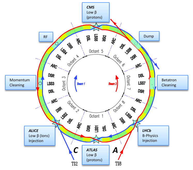
Figure 1: The general layout of the LHC [4]. The dispersion suppressors (DSL and DSR) are sections between the straight section and the regular arc. In this paper they are considered to be part of the arc, for simplicity. LSS denotes the Long Straight Section – roughly 500 m long parts of the ring without net bending. All insertions (experiments, cleaning, dump, RF) are located in the middle of these sections. Beams are injected through transfer lines TI2 and TI8. The ATLAS convention of labelling sides by ‘A’ and ‘C’ is indicated.

The LHC layout, shown in figure 1, comprises eight arcs, which are joined by Long Straight Sections (LSS) of slightly more than 250 m half-length. Each LSS houses an Interaction Region (IR) in its middle, the ATLAS detector being located in IR1. The LHC beam cleaning equipment is situated in IR3 (momentum cleaning) and IR7 (betatron cleaning), i.e. two octants away from ATLAS for beam-2 and beam-1, respectively. The role of the beam cleaning is to intercept the primary and secondary beam halo, but some protons escape, forming a tertiary halo. In order to intercept this component and to provide local protection against accidental beam losses, tertiary collimators (TCT) are placed about 150 m from the experiments on the incoming beams. The aperture settings of collimators, with respect to the nominal normalised emittance of 3.5 $\upmu{\rm m}$, are listed in table 1. It can be seen that the momentum cleaning collimators in IR3 are much more open than those of the betatron cleaning in IR7. Since most of the cleaning takes place in IR7, it has much more efficient absorbers than IR3 so that per intercepted proton there is more leakage of cleaning debris from the latter.

$\beta^{*}$	TCP in IR7 (in IR3)	TCS in IR7 (in IR3)	TCT in IR1,5 (in IR 2,8)
0.6 m	4.3 (12)	6.3 (15.6)	9.0 (12)
1000 m	2.0† (5.9†)	6.3 (15.6)	17 (26)

Table 1: Apertures of primary (TCP), secondary (TCS) and tertiary (TCT) collimators in units of nominal betatronic $\sigma$, corresponding to a normalised emittance of 3.5 $\upmu{\rm m}$ [5]. Settings for normal high-luminosity optics ($\beta^{*}=0.6$ m) and the special high-$\beta^{*}$ fill ($\beta^{*}=1000$ m), discussed in section 10.2, are given. ^†For the 1000 m optics, the given TCP settings varied and the values listed correspond to the tightest settings.

The inner triplet of quadrupoles, providing the final focus, operates at 1.9 K and extends from $z=23\,$m to $z=\,54$ m. It is equipped with a perforated beam-screen, operated at 20 K, in order to protect the superconducting coils from synchrotron radiation, electron cloud effects and resistive heating by the image currents of the passing beam. The perforation allows for residual gas to condense on the cold bore of the coils. This cryo-pumping effect is responsible for the very low pressure reached in the cold sections of the LHC [6].

The residual pressure close to the experiment is monitored by several vacuum gauges of Penning and ionisation types. The 2011 background analysis revealed that the BIB seen in ATLAS at small radius is correlated with the pressure measured at 22 m. Further gauges are at 58 m (on accelerator side of inner triplet), 150 m (close to the TCT) and $\sim$250 m (at exit of the arc) from the IP. All of these were considered in the analysis but finally only the 22 m and 58 m readings were found to show a correlation with the observed backgrounds. The gauge at 58 m is located in a short warm section without Non-Evaporative Getter coating [7]. Electron-cloud formation was discovered to be a problem in this region and already in 2011 solenoids were placed around the beam-pipe in order to suppress electron multipacting. The solenoids were found to be efficient and remained operational throughout 2012.

The inner triplet quadrupole absorber (TAS) is another machine element of importance for background formation. It is a 1.8 m long copper block located at $z=19\,$m from the interaction point (IP) with a 17 mm radius aperture for the beam. While the TAS provides a shielding effect against beam backgrounds, high-energy particles impinging on it can initiate showers that are sufficiently penetrating to partially leak through.

A few thousand beam loss monitors (BLM) are distributed all around the LHC ring in order to monitor beam losses and to initiate a protective beam dump in case of a severe anomaly. The time resolution of a BLM is limited by its electronics to about 40 $\upmu{\rm s}$, so it cannot be used to determine loss rates of individual bunches. Since the BLMs are located around very different machine elements, with different internal shielding, their response with respect to one lost proton is not uniform. Thus, without detailed response simulations, the BLMs cannot be used to compare the losses in two different locations. They serve mainly to give information about the time development of losses on a given accelerator element. The loss-rates on the TCT would be most interesting for background studies. Unfortunately, in this location, the BLMs are subject to intense debris from the collisions, so during physics operation they have no sensitivity to halo losses.

Another beam monitoring system is the Longitudinal Density Monitor (LDM), which is used to measure the population in each RF bucket by synchrotron light emission [8]. The system has sufficiently good time resolution and charge sensitivity to detect ghost charge in individual RF buckets with an intensity several orders of magnitude below the nominal bunch intensity of $\sim\!10^{11}$ protons/bunch. In 2012 the system was operational only in some LHC fills and elaborate calibration and background subtraction had to be developed in order to extract the signal.

The beam intensity is measured by two devices of which only one, the fast beam current transformer (FBCT), provides intensity information bunch by bunch. Where appropriate, the intensity values provided by the FBCT have been used to normalise backgrounds.

Normal data-taking happens in the STABLE BEAMS mode. This is preceded by phases called FLAT TOP, when beams have reached full energy, SQUEEZE, when the optics at the interaction points is changed to provide the low $\beta^{*}$ focusing for physics and ADJUST, during which the beams are brought into collision. Together FLAT-TOP and SQUEEZE last typically 20 minutes. During this time the beams remain separated, which provides particularly clean conditions for background monitoring.

2.2 The ATLAS detector

ATLAS is a general purpose detector at the LHC with almost $4\pi$ coverage. It is optimised to study proton-proton collisions at the highest possible energies, but has capabilities also for heavy-ion and very forward physics. The ATLAS inner detector is housed inside a solenoid which produces a 2 T axial field. It is surrounded by calorimeters and a muon spectrometer based on a toroidal magnet configuration. The calorimeters extend up to a pseudorapidity $|\eta|=4.9$, where $\eta=-\ln\tan(\theta/2)$, with $\theta$ being the polar angle with respect to the nominal LHC beam-line in the beam-2 direction. Charged particle tracks are measured by the inner detector in the range $|\eta|<2.5$. In the right-handed ATLAS coordinate system, with its origin at the nominal IP, the azimuthal angle $\phi$ is measured with respect to the $x$-axis, which points towards the centre of the LHC ring. As shown in figure 1, side A of ATLAS is defined as the side of the incoming, clockwise, LHC beam-1 while the side of the incoming beam-2 is labelled C. The coding of LHC machine elements uses letters L (left of IR, when viewed from ring centre) for ATLAS side A and, correspondingly, R for side C. The $z$-axis in the ATLAS coordinate system points from C to A, i.e. along the beam-2 direction. The most relevant ATLAS subdetectors for the analyses presented in this paper are the Beam Conditions Monitor (BCM) [10], LUCID, the calorimeters, and the Pixel detector.

The BCM detector consists of 4 diamond modules ($8\times 8\,{\rm mm}^{2}$ active area) on each side of the IP at a $z$-distance of 1.84 m from the IP and a mean radius of $r=5.5$ cm from the beam-line, corresponding to $|\eta|=4.2$. The modules on each side are arranged in a cross, i.e. two in the vertical plane and two in the horizontal plane. The individual modules will be referred to as Ax-, Cy+, etc. where the first letter refers to the side according to ATLAS convention, the second letter to the azimuth and the sign is according to the ATLAS coordinate system.

The LUCID detector was introduced as a dedicated luminosity monitor. It consists of 16 Cherenkov tubes per side, each connected to its own photomultiplier (PMT), situated in the forward region at a distance $z=18.3$ m from the IP, giving a pseudorapidity coverage of $5.6<|\eta|<6.0$. In 2012 LUCID was operated without gas in the tubes, most of the time. In this configuration, only the Cherenkov light from the quartz-window of a PMT was used for particle detection.

The Pixel detector consists of three barrel layers at mean radii of 50.5 mm, 88.5 mm and 122.5 mm. All layers have a half-length of 400 mm, giving an $|\eta|$-coverage out to 1.9 and 2.7 for the outermost and innermost layers, respectively. In each layer the modules are slightly tilted with respect to the tangent. The pixel size in the barrel modules is $r\phi\times z=50\times 400\,\upmu{\rm m}$. The full coverage, with three points per track, is extended to $|\eta|=2.5$ by three endcap pixel disks.

A high-granularity liquid-argon (LAr) electromagnetic calorimeter with lead as absorber material covers the pseudorapidity range $|\eta|<1.5$ in the barrel region. The half-length of the LAr barrel is 3.2 m and it extends from $r=1.5$ m to $r=2$ m. The hadronic calorimetry in the region $|\eta|<1.7$ is provided by a scintillator-tile calorimeter (TileCal), extending from $r=2.3$ m to $r=4.3$ m with a half-length of 8.4 m. Hadronic endcap calorimeters (HEC) based on LAr technology cover the range $1.5<|\eta|<3.2$. The absorber materials are iron and copper, respectively. The calorimetry coverage is extended by the Forward Calorimeter up to $|\eta|=4.9$. All calorimeters provide nanosecond timing resolution.

3 Non-collision backgrounds

The non-collision backgrounds (NCB) are defined to include CRB and BIB. The main sources of the latter are [1, 11]:

• Inelastic beam-gas events in the LSS or the adjacent arc. Simulations indicate that contributions from up to about 500 m away from the IP can be seen [12].

• Beam losses on limiting apertures. The contributions to the experiments come predominantly from losses on the TCTs, which in the normal optics are the smallest apertures in the vicinity of ATLAS.

• Elastic beam-gas scattering around the ring. According to simulations [12, 11], the scattered protons are intercepted by the beam cleaning insertions or the TCTs. In the latter case their effect adds to the halo losses on the TCTs.

Beam-gas events, within about $\pm$50 m from the IP, can spray secondary particles on the ATLAS inner detectors, but it is unlikely that they reach large radii and give signals in, e.g., the barrel calorimeters. The fake jets due to BIB, which are a major subject of this paper, are caused by high-energy muons produced as a consequence of proton interactions with residual gas or machine elements far enough from the IP to allow for the high-energy muons to reach the radii of the calorimeters. Radiative energy losses of these muons in calorimeter material, if large enough, are reconstructed as jets and can form a significant background to certain physics searches [13]. A characteristic feature of the high-energy muon component of BIB is that, due to the bending in the dipole magnets of the LHC, it is predominantly in the horizontal plane.

The CRB is entirely due to high-energy muons. These can penetrate the 60 m thick overburden and reach the experiment. Just like the BIB muons, the CRB muons can create fake jets in the calorimeters by radiative energy losses and thereby introduce backgrounds to physics searches [14].

A significant part of this paper is devoted to studies of ghost charge. The definition adopted here is to call ghost charge all protons outside the RF buckets housing nominally filled bunches. There are two different mechanisms which lead to ghost bunch formation.

• Ghost bunch formation in the injectors: Of particular interest are ghost bunches formed in the Proton Synchrotron (PS) during the generation of the LHC bunch structure. In the PS a complicated multiple splitting scheme [16] is applied on the bunches injected from the Booster (PSB). The result of this is to split a single PSB bunch into six bunches, separated by 50 ns. If any of the protons injected from the PSB do not fall into a PS bucket, the protons spilling over might be captured in an otherwise empty bucket and undergo the same splitting. In this case six ghost bunches with a 50 ns spacing will be formed. Similar spill-over can occur in the injection from the PS into the Super Proton Synchrotron (SPS). In this case ghost bunches with a 5 ns spacing can be formed. If the production mechanism is of significance in a given context, these bunches will be referred to as injected ghost bunches.

• De-bunching in the LHC: In the course of a fill, a small fraction of the protons develop large enough momentum deviations to leave their initial bucket [17]. These escaped protons can drift in the LHC for tens of minutes and complete several turns more than their starting bucket before being intercepted by the beam cleaning [17, 18]. Due to their relatively long lifetime these de-bunched protons can be assumed to be rather uniformly distributed. Some of the de-bunched charge can be re-captured by the RF forming ghost bunches all round the ring. Thus the de-bunched ghost charge maintains an imprint of the bucket structure.

4 Background monitoring methods

In the ATLAS first level (L1) trigger, the LHC bunches are grouped according to their different characteristics into bunch groups (BG). Two of these groups are of particular importance for beam background analysis: unpaired isolated and unpaired non-isolated. In the first of these groups the requirement is to have no bunch in the other beam within 150 ns, while the second group includes those unpaired bunches which fail to fulfil this isolation requirement. The timing of the central trigger is such that the collision time ($t=0$) of two filled bunches falls into the middle of the BCID. When reference to an empty BCID is made in this paper, it means any BCID without a bunch in either beam.

During each LHC fill ATLAS data-taking is subdivided into Luminosity Blocks (LB), typically 60 s in duration but some can be as short as 10 s. While recorded events carry an exact time-stamp, trigger rates and luminosity data are recorded only as averages over a LB.

4.1 Background monitoring with the BCM

Throughout LHC Run-1, the BCM was the primary device in ATLAS to monitor beam backgrounds. Gradually, the full capabilities and optimal usage of the detector were explored and allowed for refinement of some of the results obtained on 2011 data [1] and augmenting these with new studies. In this section some aspects relevant to the BCM data, taken in 2012, are presented in detail.

BCM time resolution

The time resolution of the BCM is measured to be of the order of 0.5 ns. In the readout the 25 ns duration of a BCID is subdivided into 64 bins, each 390.625 ps wide. For each recorded event, the entire vector of 64 bins is stored, allowing the exact arrival time and duration of the signal to be determined. The bins are aligned such that the nominal collision time falls into bin 27, i.e. about 2 ns before the centre of the readout interval. More details about the readout windows are given in appendix A.

BCM triggers and luminosity data

In 2012 the BCM detector provided two different L1 triggers:

• L1_BCM_AC_CA is a background-like ‘coincidence’, i.e. requires an early hit in upstream detectors associated with an in-time hit in downstream detectors. The window widths are the same as in 2011: the early window at $-6.25\,\pm\,2.73$ ns and the in-time window at $+6.25\,\pm\,2.73$ ns, where the IP-passage of the bunch is at 0.

• L1_BCM_Wide is a trigger designed to select collision events by requiring a coincidence of hits on both sides. Until the third technical stop (TS3) of the LHC in mid-September, the window setting of 2011 was used, i.e. the window was open from 0.39 ns until 8.19 ns following the collision. Since this alignment did not seem optimal for a nominal signal arrival at 6.1 ns, TS3 was used to realign it with the in-time window of the BCM_AC_CA trigger. A detailed discussion of the consequences of this realignment and reduction of window width is given in appendix A.

Another significant modification implemented during TS3 was to combine all four BCM modules per side of ATLAS into one read-out driver (ROD), where previously two independent RODs had each served a pair of modules. Consequently the L1_BCM_Wide rates recorded prior to TS3 have to be doubled to be comparable with post-TS3 trigger rates, as shown in appendix A .

The combination of all modules into a single ROD also affected the BCM_AC_CA rates, but the effect is less obvious. The correction factor for pre-TS3 rates, derived in appendix A, is 1.2.

The rates per BCID were recorded in a special monitoring database averaged over 300 s. For some of the per-BCID rate studies presented in this paper this integration time proved too long and recourse to the luminosity data from the BCM had to be made. These data, dedicated for luminosity measurement with the BCM, are available as LB-averages, i.e. with a typical time resolution of 60 s, for each BCID independently. As for the BCM triggers, the luminosity data are based on a hit in any of the four modules on one side. The time-window to accept events for the luminosity algorithms is 12.5 ns, starting at the nominal collision time. For the purpose of this paper only the single-side rates are relevant and will be denoted as BCM-TORx. By comparing BCM-TORx rates in colliding bunches, the difference in efficiency, including acceptance, between sides A and C was found to be $<$1%. Since those data are recorded independently for each side, it is not possible to reconstruct the background-like timing pattern. Consequently these data are most useful for unpaired bunches in conditions where the BIB is high compared to other signals. Such cases will be encountered in sections 10.1 and 10.2. Recourse to the BCM luminosity data will also be made in section 7.2 when describing a new method to disentangle ghost collisions from noise and BIB.

BCM data quality

A noise of unidentified origin appeared in A-side BCM modules on 27 October evening. The noise lasted until the morning of 26 November and constituted a significant increase in the level of random hits and will be clearly visible in many plots in this paper. The noise period has been excluded from analyses where it would have influenced the result. In trend plots over the year the period is included, but highlighted and in most cases should be ignored.

A few LHC fills, predominantly early in the year, were affected by various types of data quality problems, mostly loss of trigger synchronisation or beam intensity information. These fills have been removed from the analyses and the trend plots.

4.2 Using LUCID luminosity data in background analysis

The LUCID data are recorded by the luminosity data-acquisition software, independently of the ATLAS trigger and are available per BCID and LB, typically with very good statistics.

The LUCID detector is not as fast as the BCM and suffers more from long-lived collision debris, which will be discussed in section 6. Unlike in 2011, the 2012 operation had two specific cases where LUCID proved very useful to detect backgrounds. These were a normal fill with abnormally high background and the high-$\beta^{*}$ fill with very low luminosity and sparse bunch pattern, discussed in sections 10.1 and 10.2, respectively.

The use of LUCID in those special cases is made possible by its large distance from the IP, which allows the separation of the background hits from the luminosity signal. The usable signal comes from the background associated with the incoming bunch, observed in the upstream LUCID. The incoming bunch passes the upstream detector about 60 ns before the actual collision which means that the background from that bunch appears five BCIDs before the luminosity signal, twice the time-of-flight between the IP and LUCID. This is illustrated in figure 2, using data from the high-$\beta^{*}$ fill with very low luminosity and only two colliding bunches. The normal luminosity signal is seen in BCID 1886 and is of comparable size during high beam losses and in normal conditions. The background signal appears five BCID earlier and peaks in BCID 1881. In normal conditions it is much smaller than the luminosity peak, but during high losses it can become very prominent. Unlike the BCM-TORx signal, this early LUCID signal has practically no luminosity contamination even for paired bunches and lends itself very well to monitoring of the beam background of bunches with a long empty gap preceding them.

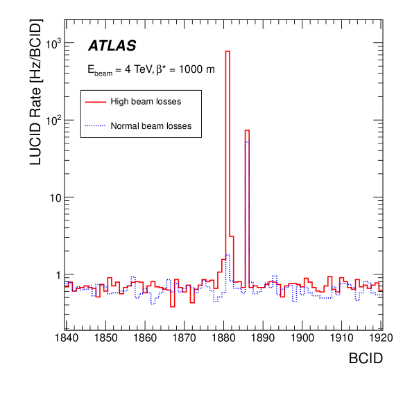
Figure 2: Background and luminosity signal seen by LUCID in the high-$\beta^{*}$ fill (discussed in section 10.2). Both data-sets average over three ATLAS luminosity blocks, i.e. about 180 s.

4.3 Using calorimeter jets in background analysis

In the analysis of 2011 backgrounds jets proved to be a useful tool to study characteristics of NCB [1]. A jet trigger L1_J10 was defined in the 2012 data-taking for unpaired bunches in order to select BIB events with fake jets. The L1_J10 trigger fires on a transverse energy deposition above 10 , calibrated at approximately the electromagnetic energy scale [19], in an $\eta$–$\phi$ region with a width of about $\Delta\eta\times\Delta\phi=0.8\times 0.8$ anywhere within $|\eta|<3.0$ and, with reduced efficiency, up to $|\eta|=3.2$. A similar trigger with a 30  transverse energy threshold, L1_J30, was defined for recording CRB data.

In order to suppress instrumental backgrounds that are not due to BIB or CRB, abrupt noise spikes are masked during the data reconstruction and efficiently removed by the standard data quality requirements [20].

For an offline analysis of the recorded data, the anti-$k_{t}$ jet algorithm [21] with a radius parameter $R=0.4$ is used to reconstruct jets from the energy deposits in the calorimeters. The inputs to this algorithm are topologically connected clusters of calorimeter cells [19], seeded by cells with energy significantly above the measured noise. These topological clusters are calibrated at the electromagnetic energy scale, which measures the energy deposited by electromagnetic showers in the calorimeter. The measured jet transverse momentum is corrected for detector effects, including the non-compensating character of the calorimeter, by weighting energy deposits arising from electromagnetic and hadronic showers differently. In addition, jets are corrected for contributions from pileup, as described in reference [19]. The minimum jet transverse momentum considered is 10 .

The jet time is defined as the weighted average of the time of the calorimeter cell energy deposits in the jet, weighted by the square of the cell energies. The calorimeter time is defined such that it is zero for the expected arrival of collision secondaries at the given location, with respect to the event time recorded by the trigger.

4.4 Pixel background tagger

In the course of the 2011 background analysis [1], an algorithm was developed to tag beam background events based on the presence of elongated clusters in the Pixel barrel layers. While collision products, emerging from events at the IP, create short clusters at central pseudorapidities, the clusters due to BIB, with trajectories almost parallel to the beam pipe, create long clusters at all $\eta$ in the Pixel barrel. At high $|\eta|$ the clusters from $pp$ collision products in the barrel modules also become long, so the tagging method has its best discrimination power below $|\eta|\sim 1.5$.

5 Data-taking Conditions

In 2012 the LHC collided protons at $\sqrt{s}=8\,$, i.e. with $4\,$ energy per beam. Except for some special fills, the bunch spacing was 50 ns which allowed for slightly fewer than 1400 bunches per beam. The typical bunch intensity at the start of a fill varied between $1.2\!-\!1.7\!\times\!10^{11}$ protons. Most of 2012 physics operation was at $\beta^{*}=0.6$ m. In order to avoid parasitic collisions a crossing half-angle of 145 $\upmu{\rm rad}$ between the two proton beams was used. The normalised emittance was typically around 2.5 $\upmu{\rm m}$ which is well below the nominal value of 3.5 $\upmu{\rm m}$.

The colliding bunches were grouped into trains with $2\!-\!4\times 36$ bunches, with a separation of 900 ns between the trains to allow for the injection kicker rise time. Within these long trains the 36 bunch sub-trains were separated by nine empty BCIDs.

Since backgrounds depend on beam conditions, they are expected to be different for various beam structures. The beam pattern of 2011, with 1331 colliding bunches, was used at the beginning of 2012 data-taking until instabilities of the unpaired bunches [22] required finding a different filling scheme. The intermediate solution was a 1377 colliding bunch pattern with only three unpaired bunches per beam, which were all non-isolated according to the ATLAS standard definition. In order to retain one bunch in the unpaired isolated group, which is used primarily for background monitoring, it was decided to relax the isolation requirement from 150 ns to 100 ns. Continuing instabilities led the LHC to introduce temporarily a fill pattern with 1380 colliding bunches, leaving none unpaired. During this period, lasting from 24 May until 5 June, there was no background monitoring capability. After optimisation of the LHC machine parameters, the unpaired bunches could be reintroduced and soon afterwards (from LHC fill 2734 onwards) an optimal fill pattern was implemented. This pattern with 1368 colliding bunches has a mini-train of six unpaired bunches per beam in the ideal location, immediately after the abort gap in odd BCIDs 1–11 and 13–23. In this pattern the first colliding train started in BCID 66 and the last colliding bunch before the abort gap was in BCID 3393. Initially the beam-1 mini-train was first, but at the end of the year (24 November, from LHC fill 3319 onwards) the trains were swapped in order to disentangle possible systematic beam-1/beam-2 differences and effects caused by the relative order of the unpaired trains.

Period	Colliding	Unpaired (non-)isolated per beam	Dates
1	1331	(40)9	18.4. – 19.5.
2	1377	(2)1	19.5. – 24.5. & 5.6. – 15.6.
—	1380	(0)0	24.5. – 5.6
3	1368	(3)3	15.6. – 17.9.
4	1368	(3)3	29.9. – 6.12.

Table 2: Periods with different numbers of colliding and unpaired bunches. Periods 3 and 4 are separated by TS3 during which changes to the BCM trigger logic were implemented. Since the pattern with 1380 colliding bunches had no unpaired bunches, background monitoring in that period was not possible.

All periods described above are listed in table 2. The period with 1368 colliding bunches is divided into pre-TS3 and post-TS3 periods because the BCM trigger rates are not directly comparable, as discussed in appendix A. In addition, there were several fills with special bunch structure early in 2012 and a few such fills appeared also later in the year. Many of these were dedicated fills, e.g. for van der Meer scans, high-luminosity or 25 ns tests. Since these fills do not share common characteristics, they are not included in the trend plots presented in this paper.

At the high beam intensities reached in 2012 and with 50 ns bunch spacing, outgassing from the beam pipe becomes a significant issue for the vacuum quality. Special scrubbing fills at $450\,$ beam energy but high intensity were used in early 2012 to condition the beam pipe surfaces. Despite these special fills some vacuum conditioning most likely continued throughout the first months of physics operation.

Characteristics	Dates
BCM
Before chromaticity changes	15.6. – 3.8.
From chromaticity changes until BCM Noise	10.8. – 27.10.
After BCM Noise	26.11. – 6.12.
Jets
Before chromaticity changes	15.6. – 3.8.
From chromaticity changes until unpaired swap	10.8. – 24.11.
After unpaired swap	25.11. – 6.12.

Table 3: Break-points, which had significant influence on rates or data quality for background monitoring based on BCM (top) and jets (bottom), during 2012 data taking with 1368 colliding bunches. Within a given period data from different fills should be comparable.

As will be seen, an event of significance for some analyses in this paper was when LHC changed chromaticity settings between 3–9 August. During this period, extending over several days, the LHC was optimising performance with different chromaticities and a switch of octupole polarities on 7 August.

All the break-points marking the important changes during the data-taking with 1368 colliding bunches, leading to significant changes in background rates or influencing the data quality, are summarised in Table 3. Periods 1 and 2 of Table 2 are not mentioned there since those early periods have very different bunch patterns and have to be treated separately. No particular events, aside from the pattern changes, were identified during those periods.

6 Afterglow

The term afterglow was introduced in the context of the ATLAS luminosity analysis [23] to describe signals caused by delayed tails of particle cascades following a $pp$ collision. The afterglow decreases rapidly over the first few BCIDs following a collision, but a long tail extends up to about 10 $\upmu{\rm s}$, as a result of which significant afterglow buildup is observed in colliding trains, with 50 ns bunch spacing. In the region of the long tail, more than $\sim$100 ns after the last paired bunch crossing, the afterglow hits appear without any time-structure and are thus indistinguishable from instrumental, or other, noise.

In the rapidly dropping part immediately after the collision the distinction between prompt signal and afterglow is somewhat ambiguous. A natural definition for the afterglow from $pp$ collisions is to consider as prompt all hits with a delay less than the BCID half-width of 12.5 ns, while the rest is being counted as afterglow.

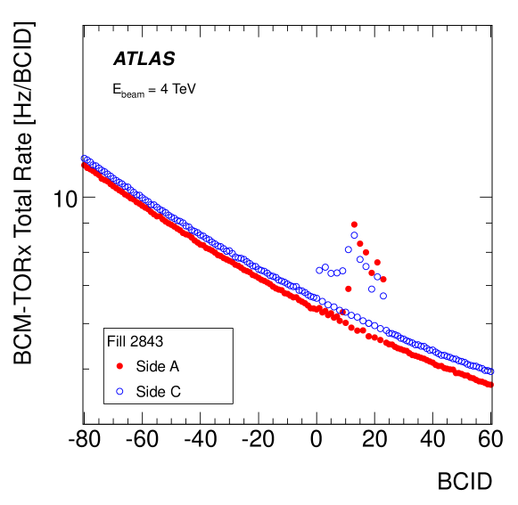
Figure 3: Afterglow distribution, as seen by the BCM-TORx algorithm, at the end of the abort gap and in the region of the unpaired bunches. The signals associated with the unpaired bunches are seen in odd BCIDs from 1 to 23. The asymmetry of the rate distribution in them will be discussed in section 7.2. For the purpose of plotting the BCID numbers in the abort gap have been re-mapped to negative values by BCID = BCID_true - 3564.

Figure 3 shows the afterglow tail created by the colliding trains before the abort gap in a normal physics fill and extending all the way to the unpaired bunches in odd BCIDs 1–23. Since the rates are much lower than one count per bunch crossing, the afterglow contribution to the unpaired bunches can be removed by subtracting the rate in the preceding BCID from that in the BCID occupied by the unpaired bunch.

In analogy to the afterglow following $pp$ collisions, there should be delayed debris from a BIB event, which will be referred to as afterglow_BIB. The component of the afterglow_BIB which arrives within the same BCID as the unpaired bunch is particularly significant for some observations to be discussed in this paper. This part has a very non-uniform, rapidly dropping, time distribution within the BCID and cannot be easily subtracted. The afterglow_BIB level is a small fraction of the primary beam-gas rate, i.e. the rate seen as in-time hits in the downstream modules. However, since the afterglow_BIB is correlated with the beam-gas events, there will be a bias towards primary beam-gas and afterglow_BIB signal to form a collision-like coincidence, i.e. provide real and apparent in-time hits on both sides of the IP. In order for this to happen the afterglow has to arrive at the upstream detectors with a delay corresponding to the time-of-flight between the two BCM detector arms, i.e. about $12.5\,$ns $\pm\Delta t$. Here, $\Delta t$ is the tolerance allowed by the coincidence trigger window. If the downstream signal is exactly in time, $\Delta t=2.7\,{\rm ns}$ for L1_BCM_Wide after TS3 and 6.3 ns for observing simultaneous BCM-TORx signals on both sides.

Since the afterglow_BIB signal is very small, the overwhelming afterglow from the collisions prevents extracting it from stable-beam data. However, around 20 minutes of data at the start of each fill is obtained during the FLAT-TOP and SQUEEZE phases, in which the full-energy beams are separated and so there is no large afterglow from collisions. Figure 4 shows the BCM-TORx rates for unpaired bunches and empty BCID around them, averaged over most fills with the 1368 colliding bunch structure. Only fills until the start of the BCM noise period are included. It is clearly seen that the background noise (BCIDs$<$1 and BCIDs$>$23) is low and BCID-independent.

In addition to the primary beam-gas signals, there are additional smaller signals in the upstream modules. These are the hits from afterglow_BIB. The afterglow_BIB signals are not easily identified in figure 4 because they are barely above the noise level, which is different for the two sides. Also, the primary beam-gas signals themselves disagree by about 28%, i.e. much more than the efficiency difference of the two sides. This discrepancy reflects a real difference in beam background, possibly due to systematically worse vacuum on side A. These arguments motivate processing the data by first subtracting the background noise and then rescaling one beam such that the primary BIB signals match. For each beam the noise level is determined as an average over 20 empty BCIDs preceding the first unpaired bunch. The rates in BCID 13–24 are multiplied by a factor of 1.28 in order to bring the primary BIB signals on the two sides into agreement.

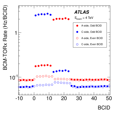
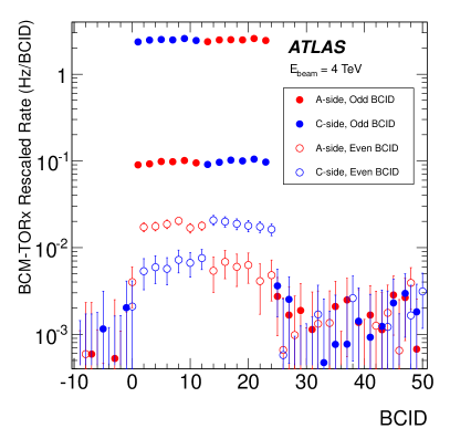
Figure 4: Single sided BCM-TORx rates of unpaired and empty bunches during periods with separated full energy beams before (a) and after (b) noise subtraction and rescaling to match the primary beam-background rates of both beams, as explained in the text. For clarity, signals in odd and even BCIDs are shown with different symbols. The unpaired bunches are all in odd BCIDs.

The rates after these adjustments are shown in figure 4, where two levels of signal rate in odd BCIDs on sides A and C are seen to match each other. The perfect agreement of the second level, around 0.1 Hz/BCID, after simply matching the primary BIB rates ($\sim$2.5 Hz/BCID) on the two sides, means that it is proportional to the primary BIB rate at a level of 3.9% thereof, which leaves little doubt about its interpretation as afterglow_BIB signals.

In figure 4 the factor 1.28 is applied also to the empty (even) BCIDs in the range 14–24 between beam-2 bunches. It is not evident if this is justified since the origin of the signals in them is not certain. A contribution from beam-1 ghost charge cannot be excluded. The statistical uncertainties on those points are large enough for the two sides to agree both with and without scaling.

In order to avoid confusion between afterglow_BIB, which is important only because of its correlation with BIB events, and the much more significant level of afterglow from $pp$ collisions, the latter will be referred to as afterglow_pp.

The excellent time resolution of the BCM signal and data acquisition system enabled the arrival time of the background to be measured precisely. By exploiting the fine time binning of the recorded BCM signal, the existence of an afterglow_BIB tail was verified and its shape was studied in detail. Figure 5 shows the time distributions in two BCM modules in events triggered by the L1_BCM_AC_CA trigger on unpaired isolated bunches of either beam. For beam-1 a pronounced early peak on the A-side is observed in figure 5, corresponding to the background associated with the incoming bunch. It is followed by a long tail, consistent with afterglow_BIB. Beam-1 exits on the C-side and correspondingly the peak appears around bin 43, i.e. ‘in-time’ with respect to the nominal collisions, again followed by a tail due to afterglow_BIB. In figure 5 similar structures are seen for beam-2, but on the opposite sides.

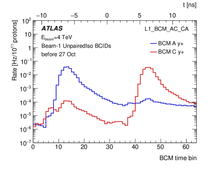
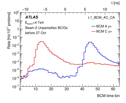
Figure 5: Response of the BCM $y+$ station in the BCIDs defined for beam-1 (a) and beam-2 (b) in the events triggered by L1_BCM_AC_CA_UNPAIRED_ISO. Data with 1368 colliding bunches until the BCM noise period are used.

However, there are also some entries consistent with early hits in downstream modules. A flat, or slowly falling, pedestal is expected from noise and afterglow causing random triggers. But instead clear peak-like structures are seen in figure 5, especially in unpaired BCIDs of beam-1. These can be attributed to ghost bunches in the other beam, but a detailed discussion is deferred to section 9.

7 Background monitoring

7.1 Beam-gas events

The analysis of 2011 background data revealed a clear correlation of the beam background as seen by the BCM and the residual gas pressure reported by the gauges at 22 m. Using the data from a dedicated test fill without electron-cloud suppression by the solenoids at 58 m, the contribution of the pressure at 58 m to the observed background was estimated to be 3–4 % [1].

In 2012 no such dedicated test was performed, but the contributions of various vacuum sections were estimated by fitting the background (${\rm BIB}_{\rm BCM}$) data with a simple 3-parameter fit:

$${\rm BIB}_{\rm BCM}=A(f\cdot p22+(1-f)\cdot p58)+b,$$ (1)

where $p22$ and $p58$ are the pressures measured at 22 m and 58 m, respectively, and $A$, $f$ and $b$ are free parameters. The constant $b$ is introduced to take into account any background not correlated with the two pressures included in the fit. Since ${\rm BIB}_{\rm BCM}$ is normalised by bunch intensity, the fit implies that also $b$ is assumed to be proportional to beam intensity, which is a valid assumption if $b$ is due to beam-gas further upstream. However, if a residual contribution comes from beam-halo losses or noise, it is not necessarily proportional to intensity.

The pressure values given by the three gauges, available at 22 m, were not always consistent. If information from an individual gauge was not received for a short time interval, the gap was bridged by using the last available value, provided it was in the same fill and not older than 10 minutes. Obviously erratic readings were rejected by requiring that the value was within a reasonable range ($10^{-11}$ – $10^{-6}$ mbar). The pressure was determined by first taking the average of the pair of readings closest to each other and including the value from the third gauge only if it did not deviate by more than a factor of three from this pair-average. Such a three-gauge average was accepted in 97% of luminosity blocks and in only 0.3% of cases a two-gauge average was used. The number of cases that all gauges deviated by more than a factor of three from each other negligible. In 2.7% of luminosity blocks no valid pressure data could be determined and the luminosity block was ignored.

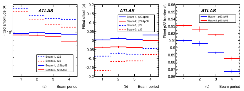
Figure 6: Parameters $A$ (a), $b$ (b) and $f$ (c), resulting from the fit of equation 1 to data in periods 1–4, as detailed in table 2.

Figure 6 shows the obtained fit parameters for the periods listed in table 2 using either $p22$ only, i.e. $f=1.0$, or a combination of $p22$ and $p58$ in Eq. 1. It can be seen that the value of $A$, which corresponds to the absolute normalisation, is systematically lower for beam-2, which implies that for the same measured pressure there is less background from beam-2 than beam-1. The difference varies over the year, but is roughly 20% during the operation with 1368 colliding bunches (periods 3 and 4). The two sides of ATLAS are symmetric, so there is no obvious explanation why the backgrounds should be different. However, this difference in the fitted $A$ is close to the 28% that was derived from figure 4.

Ideally, the offset $b$ should reflect how well the pressures alone describe ${\rm BIB}_{\rm BCM}$. If $b$ vanishes, it implies that there is no additional source contributing significantly, while $b>0$ means that not all sources are included in the fit. Using $p22$ only results in $b$-values which are negative by a significant amount. These have no obvious physical interpretation and indicate that a linear fit using a single pressure is insufficient to describe the data. Using both, $p22$ and $p58$, clearly improves the model and results in $b$-values more consistent with zero.

The fraction $f$ indicates how large a role $p22$ plays in explaining the observed background. The values gradually decrease during the year, but remain in a band of $90\pm 4$%, confirming the result for 2011 operation, that the background seen by the BCM is strongly correlated with the pressure at 22 m.

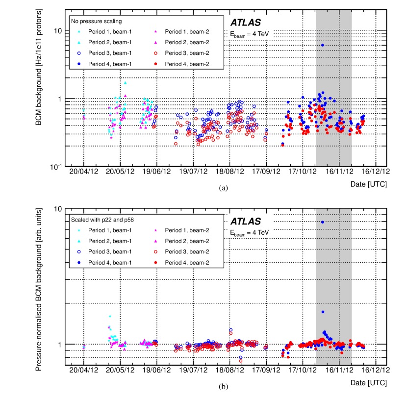
Figure 7: BCM background rate for both beams normalised by bunch intensity (a) and after an additional normalisation with the pressures at 22 m and 58 m (b) using Eq. 1 with the parameters as shown in figure 6. The shaded area indicates the period when the BCM was noisy.

Figure 7 shows the intensity normalised BCM backgrounds for both beams separately before and after scaling with the residual pressures using a fit with $p22$ and $p58$ and parameter values shown in figure 6. It should be remarked, however, that a similar plot using only $p22$ for scaling would be almost indistinguishable from figure 7(b). By construction, the scaling with equation 1 will result in an average of 1.0 in figure 7(b). The remarkable feature is that by this scaling the fill-to-fill scatter is almost entirely removed, despite the fact that the parameters are fitted over four long periods, covering most of the year.

The background estimates for beam-1 and beam-2, shown in figure 7(a), for the period with 1368 colliding bunches lead to a beam-1/beam-2 ratio of $1.21\pm 0.17$, which is perfectly consistent with the difference obtained before for the fitted parameter $A$. This ratio is also consistent with the factor 1.28 derived from non-colliding beam data in section 6, which suggests that vacuum conditions, i.e. beam-gas event rates, do not significantly change when beams are brought into collision. Since neither figure 4, nor figure 7(a), involves a pressure measurement, these good agreements suggest that the difference observed in parameter $A$ is not caused by different calibration of the gauges, but by a real difference in backgrounds. One possibility is that the pressure on side A has a different profile than that on side C and therefore the pressure gauges at 22 m do not have the same response in terms of average pressure in the region that contributes to the background.

7.2 Ghost collisions

The rate of ghost collisions, i.e. $pp$-collisions in encounters of unpaired and ghost bunches, can be estimated from the rate of events recorded by the L1_J10 and L1_BCM_Wide triggers in unpaired bunches. An independent method is to use the luminosity data from the BCM, which are recorded at high rate independently of the ATLAS trigger. In particular, the single-sided BCM event counting, BCM-TORx, as described in section 4.1 can be used. In the following, both methods will be presented and results compared.

Ghost collision rates from recorded events

From June 2012 onwards L1_BCM_Wide and L1_J10 were both run without prescale on unpaired isolated and unpaired non-isolated bunches. A significant fraction of the raw L1_BCM_Wide and L1_J10 trigger rates in unpaired bunches are due to accidental coincidences or, in the case of the latter, fake jets due to BIB muons. In this analysis ghost collisions are selected offline from the recorded event data by requiring the presence of a reconstructed vertex in a volume consistent with the luminous region and with at least two associated tracks. In order to estimate the rates correctly, the vertex reconstruction efficiency has to be known. A method for estimating this from data for L1_BCM_Wide will be presented. Luminosity blocks, or entire fills, that do not meet general data quality requirements are removed from the analysis.

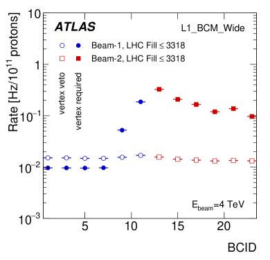
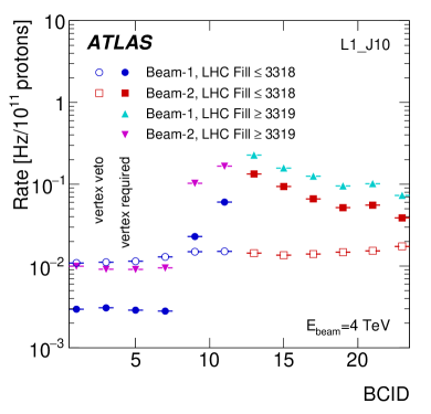
Figure 8: Left: rate of L1_BCM_Wide triggered events in unpaired BCIDs for the period prior to swapping the unpaired bunches. The solid symbols show the rate after vertex requirement and the open symbols with a vertex veto. Right: rate of L1_J10 triggered events in the same period, and after swapping the unpaired trains.

Figure 8 shows the L1_BCM_Wide rates for events with and without a reconstructed vertex. The asymmetry of the ghost collision rate is striking. As expected, the rate is much higher for lower isolation – but only for the first unpaired train, i.e. beam-1. For the second train, comprising unpaired bunches in beam-2, the rates remain high even for isolated bunches. This asymmetry arises from the beam extraction from the PS, where the kicker is timed to the start of the unpaired train, but will also extract any possible trailing ghost bunches. As a result the unpaired trains systematically have more intensity in trailing than heading injected ghost bunches. The L1_J10 rates shown in figure 8 confirm this shape. The plots also show that the unpaired isolated definition of having no bunch within 3 BCID in the other beam is adequate for the first train, while it includes a non-negligible tail of ghost collisions in the second train. This feature is preserved also after swapping the unpaired trains late in 2012, i.e. depends on the order of the trains and not on the beam.

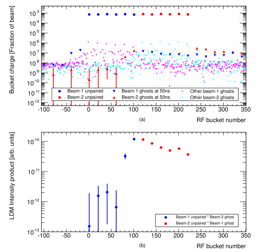
Figure 9: Charge in individual RF buckets (a) as measured by the LDM in LHC fill 3005. The buckets corresponding to the 50 ns beam structure are shown by the larger symbols. The signal of each bucket has been normalised by the sum of signals from all buckets of the beam. The product (b) of the bucket charges in beam-1 and beam-2.

The ghost collision rates seen in figure 8 are a product of ghost and unpaired bunch intensities in colliding RF buckets. These quantities can be directly measured by the LDM and the results for one of the fills when the system was operational are shown in figure 9. Figure 9(a) shows the charge in individual buckets and confirms the higher intensity of trailing injected ghost bunches and their 50 ns spacing. As explained in section 3, this is due to spill-over in the PSB to PS injection. Figure 9(b) shows the product of the bucket charges and largely confirms the shape seen in figure 8. The small differences, especially for bucket 101 (BCID 11), are likely to be explained by fill-to-fill differences, since figure 9 shows a single fill, while figure 8 is a long-term average. The point in RF-bucket 81 falls into the LDM trigger reset and had to be estimated from the value in bucket 101 using the ratio of the corresponding positions in front of other bunch-trains.

The rates with vertex veto, shown in figure 8, are almost BCID-independent, consistent with their origin being random coincidences of hits – or noise in the case of jets – which are distributed uniformly in time. However, a barely visible hump in the centre (around BCID 11) can be identified, which is due to real collisions where vertex reconstruction has failed. Assuming that the probability of fake vertex reconstruction and the vertex reconstruction inefficiency are both small, the latter can be estimated from the relative sizes of the small and the large peaks in figure 8. This yields an estimate of 1.1 % for the vertex reconstruction inefficiency. It must be emphasised, however, that this is the value with respect to collision events seen by the BCM and not a global inefficiency of ATLAS vertex reconstruction. Furthermore, a comparison of the flat tails in figure 8, taking into account this inefficiency, provides an estimate of 1.27 for the beam-1/beam-2 ratio of BIB, which is perfectly consistent with the factor 1.28 derived in section 6 and $1.20\pm 0.17$ found in section 7.

The ghost collision rate during 2012 operation is shown in figure 10, where it can be seen that the rate is rather constant until TS3 but rises steeply thereafter. L1_BCM_Wide and L1_J10 rates exhibit a similar rise, both in terms of shape and relative magnitude. Since the BCM and the calorimeters are totally independent and look at very different observables, it is not conceivable that the rise would be due to an increase of some random contribution. Thus, the identical rise must mean that the intensity of injected ghost bunches, colliding with the unpaired bunches, increased rapidly after TS3.

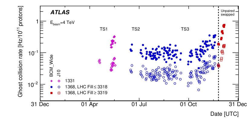
Figure 10: Ghost collision rate in unpaired bunches in the 2012 data, estimated from events triggered by L1_BCM_Wide and L1_J10 triggers. In both cases the presence of at least one reconstructed vertex is required. The early BCM points are not included, since the device was not properly timed in. The technical stops are indicated in the plot.

Ghost collision rates from luminosity data

The single-sided event rate, BCM-TORx, is composed of three contributions

$${\rm Rate}={\rm Collisions}+{\rm BIB}+{\rm Pedestal},$$ (2)

where the last term is defined to include both instrumental noise and afterglow_pp. As shown in figure 3 this pedestal can be estimated from the BCID before the unpaired bunch.

Prompt secondaries from upstream BIB events will not be counted in the upstream detector, since they arrive before the BCM-TORx window is open. A possible contribution of backscattering from beam-gas events to upstream detectors is strongly suppressed by timing and the good vacuum close to the IP. The only process, besides $pp$-collisions, which can give in-time hits in upstream detectors is the afterglow_BIB, discussed in section 6. From this argumentation, and Eq. 2, it follows that after pedestal subtraction, essentially all of the rate observed for unpaired bunches in the upstream BCM detector must be due to ghost collisions and afterglow_BIB, the latter being proportional to the primary BG signal seen in the downstream modules.

The procedure to separate the single-side BCM rate into its three components, and the results obtained, are illustrated in figure 11. In figure 11(a) the open symbols indicate that the raw BCM-TORx rate is dominated by the pedestal and the other contributions are barely visible. A clear structure, resembling figure 8 appears when the pedestal is subtracted, so that the data contain only beam-background and ghost collisions. The downstream modules are timed to see the primary BIB and ghost collision products emitted in the direction of the unpaired bunch, while the upstream modules see the ghost collision secondaries emitted in the direction of the ghost bunch and a contribution from afterglow_BIB. In figure 4 the latter was estimated to be a fraction $f=0.039$ of the primary BIB signal. Thus the rates seen in the upstream ($R_{u}$) and downstream ($R_{d}$) detectors can be written as:

$$R_{u}=fB+G$$ (3)

and

$$R_{d}=B+G,$$ (4)

where $B$ stands for the primary rate from BIB and $G$ for the rate from ghost collisions and the detection efficiencies are assumed to be identical on both sides. The equations can be solved to yield

$$B=\frac{R_{d}-R_{u}}{1-f}$$ (5)

and

$$G=\frac{R_{u}-fR_{d}}{1-f}.$$ (6)

It is worth to note that the value of $f$ is small and in the limit $f\rightarrow 0$ the equations simplify to $G=R_{u}$ and $B=R_{d}-R_{u}$, i.e. the upstream detector measures the ghost collision rate and the difference between downstream and upstream detectors gives the rate due to BIB. Figure 11(b) shows all the background components separated.

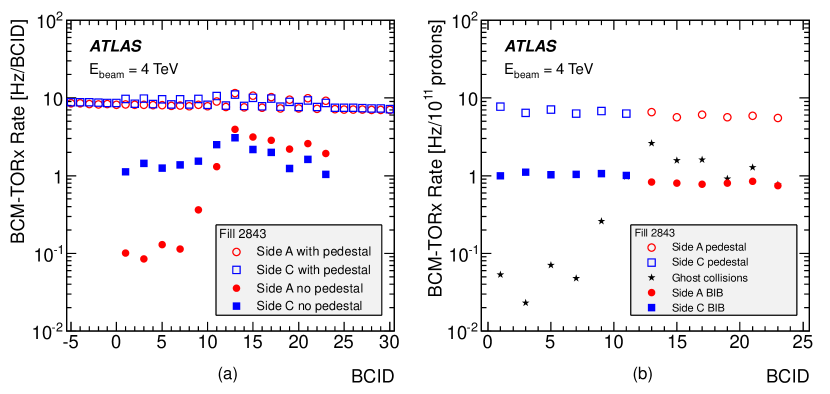
Figure 11: The procedure of separating the background components in unpaired bunches. The open symbols in plot (a) show the total single-sided rate seen by the BCM while the solid symbols show the data after subtraction of the background and restricted to the BCID-range of the unpaired punches. Plot (b) shows the three background components separated, as explained in the text.

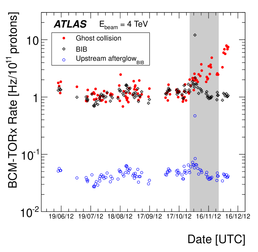
Figure 12: The BCM-TORx rate in unpaired bunches due to BIB, afterglow_BIB and ghost collisions for all 2012 fills with 1368 colliding bunches. Only the first 100 LB ($\sim 100$ minutes) of stable beams in each fill have been used in order to remove fill-length dependence.

Figure 12 compares the BCM-TORx rates, i.e. the components of Eqs. 3 and 4, due to ghost collisions ($G$), BIB ($B$) and afterglow_BIB ($fB$) for all fills in 2012 which had 1368 colliding bunches. It can be seen that for most of the year, beam-gas and ghost collisions, i.e. genuine luminosity, contribute about the same amount to the BCM-TORx rate in unpaired bunches, but at the very end of the year there is a steep rise in the ghost collision rate and it becomes the dominant contribution. This result implies that if the rate seen in unpaired bunches is used as background correction to a BCM-based luminosity measurement in a high-luminosity fill, a detailed decomposition, as described here, must be done in order to separate out the ghost collision contribution.

Having presented two different methods to monitor ghost collision rates, a comparison between the results remains to be done. The fake ghost collision triggers, i.e. coincidences without a real collision, are a sum of many independent contributions and therefore provide the most sensitive basis for comparison.

Assuming that $B$ in Eq. 5 and the pedestal are uncorrelated between sides A and C, the random coincidence rates can be obtained by simple multiplication. The rate of these fake ghost collisions should be the same as that obtained from the event-by-event analysis after applying a vertex veto. Since the pedestal is uniformly distributed in time, the different window widths of the BCM_Wide trigger and the luminosity trigger have to be taken into account, as detailed in appendix A.

The problematic component of the non-collision L1_BCM_Wide rate is the afterglow_BIB, because it does not fulfil the requirement of being uncorrelated with $B$ on the other side. Unfortunately figure 4 only determines the total afterglow_BIB rate to be about 3.9% of $B$ but does not give any information about the correlation between $B$ and afterglow_BIB signals, i.e. how often the latter coincides with the former.

If the L1_BCM_AC_CA triggered sample were an unbiased subset of BIB events giving a signal in the downstream detector, the correlation could be estimated as the fraction of L1_BCM_AC_CA triggered events, which are also triggered by L1_BCM_Wide, but have no vertex. However, the events selected by L1_BCM_AC_CA are likely to be biased towards higher multiplicities with respect to BIB events giving only downstream hits. A higher multiplicity will also imply a higher likelihood to obtain a L1_BCM_Wide trigger due to an associated afterglow_BIB hit. Thus the observed fraction of 1.3% should be considered an upper limit.

A better method to estimate the correlation is to require that the estimated rate agrees with that of events recorded by the L1_BCM_Wide trigger, after applying a vertex veto. The best match over all 2012 is obtained when 0.9% of the downstream beam-gas hits are assumed to be in coincidence with an upstream afterglow_BIB hit. Being slightly lower than the 1.3 %, this value is considered perfectly reasonable.

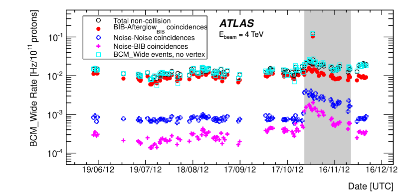
Figure 13: The total non-collision rate in the BCM_Wide trigger for 2012 LHC Fills with 1368 colliding bunches and the individual contributions to this rate. The open circles include a contribution of real ghost collisions due to the 1.1% vertex inefficiency. The jump in the pedestal-related components is due to the appearance of the BCM noise (shaded area), which then gradually decreased. Only the first 100 LB ($\sim 100$ minutes) of stable beams in each fill have been used in order to remove fill-length dependence due to the decreasing afterglow.

When this coincidence fraction of 0.9% is applied to all fills of 2012 with 1368 colliding bunches, the non-collision BCM_Wide rate estimates shown in figure 13 are obtained. The plot is consistent with the assumption that most of this rate comes from a coincidence formed by BIB and its associated afterglow_BIB. The open circles in figure 13 are the sum of the three other components shown with the addition of 1.1% of ghost collisions in order to take into account the vertex reconstruction inefficiency. Inclusion of this small fraction of ghost collisions is needed to describe the rise towards the end of the year. An agreement of the open circles and open squares is enforced on average by the matching of the data, as described above. This procedure, however, does not constrain agreement of the fill-to-fill fluctuations or the slight rise over the year. For both very good consistency between the two methods is observed.

8 Fake jets

Muons can emerge from the particle showers initiated by beam gas interactions or scattering of the beam halo protons at limiting apertures of the LHC. Such BIB muons, with energies potentially up to the range, may enter the ATLAS calorimeters and deposit energy which is then reconstructed as a fake jet. The simulations of BIB show that the high-energy muons leading to fake jets at radial distances of $R>1$ m, originate from the tertiary collimators or, in the case of beam-gas collisions, even further away [1, 11].

Nearly every physics analysis in ATLAS requires good quality jets with the pile-up contribution suppressed and non-collision backgrounds removed. In reference [1] various sets of jet cleaning criteria were proposed to identify NCB. Since then, these have been commonly used in ATLAS analyses. While calorimeter noise appears at a rate low enough to not significantly increase the trigger rate, calorimeter hot cells, BIB and CRB-muons may take up a significant fraction of the event recording bandwidth. The number of events triggered by a fake jet and entering a given analysis, strongly depends on the event topology considered. Single-jet selections are most likely to pick up a fake jet on top of minimum-bias collisions that happen during every crossing of two nominal bunches. Therefore, analyses with jets and missing transverse momentum () in the final state, such as the mono-jet analysis [13], crucially depend on an efficient jet-cleaning strategy. More complicated topologies will include NCB only if it is in combination with other hard collision products.

This section reports on the observation of fake jets due to BIB muons in unpaired bunches as well as the ones extracted from collision data by inverting the jet cleaning selection. In addition, the rates of fake jets due to CRB muons are compared to a dedicated Monte Carlo simulation. Finally the rates of fake jets due to BIB and CRB are compared as a function the $p_{\rm T}$ of the reconstructed jet.

8.1 Fake jets in unpaired bunches

Unpaired bunches provide a unique environment for studying fake jets due to BIB muons. For such analysis, the recorded events triggered by L1_J10 are selected from a dataset satisfying general data quality conditions, as described in section 4.3. Jets emerging from ghost collisions are efficiently suppressed by a vertex veto.

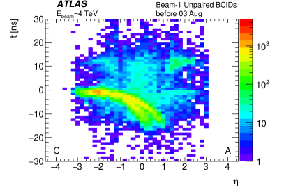
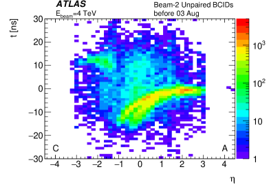
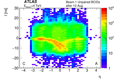
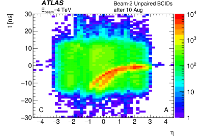
Figure 14: Jet times as a function of $\eta$ in unpaired BCID before 3 August (a,b) and after 10 August (c,d). The (a,c) and (b,d) show unpaired BCIDs for beam-1 and beam-2, respectively. Only fills with 1368 colliding bunches are considered. Negative $\eta$ corresponds to side C, i.e. outgoing beam-1.

Figure 14 shows the characteristic “banana”-shape signature in the $\eta$–$t$ plane of the distribution of fake jets due to BIB muons that traverse the detector from one side to the other. The curvature of the “banana” depends on the radial position in the calorimeter [1]. The larger curvature corresponds to the Tile calorimeter, the other tail is due to jets in the LAr calorimeter. The jet time reconstruction is adjusted such that ideally $t=0$ is found for all jets originating in a $pp$ collision. At higher $|\eta|$ on the downstream side a small residual offset of approximately $-1\,$ns is observed because the BIB muons travel parallel to the beam and therefore reach any given position in the calorimeters earlier than the collision products. The time-distributions are cut off around $\pm 12.5\,$ns due to the 25 ns acceptance of the trigger within a BCID.

The data in figure 14 are shown separately for periods before early August (a, b) and after mid-August (c, d). The motivation for this separation is related to the chromaticity changes of the LHC, which cause significant differences to the fake jet distributions in the $\eta$–$t$ plane:

• In data before early August the “banana” shapes are clearly distinguished against a low background. In addition a concentration of jets at $|\eta|\sim 2$ and $t\sim 10$ ns can be seen. These are caused by upstream fake jets in the following bunch which arrives 50 ns later, i.e. for the proper bunch crossing they would appear at $t\sim-40$ ns, but such an early arrival means that they fall into the trigger window two BCIDs earlier.

• After mid-August, most structures are masked by an almost uniform pedestal covering the entire area in the $\eta$–$t$ plane, where jets are reconstructed. An analysis of the azimuthal distribution of this pedestal revealed that it exhibits the characteristic $\phi$-structure of beam backgrounds [1], which suggests that it is not random noise or afterglow_pp, but real background. This suggests significantly higher levels of background from de-bunched ghost charge after the chromaticity changes, which will be further discussed in section 9.

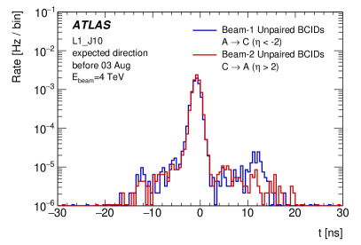
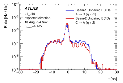
Figure 15: Jet times for fake jets at $|\eta|>2$ without a reconstructed vertex for the period before 3 August (a) and between 10 August and the swap of the unpaired trains (b). Only fills with 1368 colliding bunches are considered. The plots are normalised by the live-time, the rate is averaged over the six unpaired BCIDs per beam and the bin width is 0.5 ns.

The explanation for an almost uniform jet distribution in the $\eta$–$t$ plane comes from the fact that the de-bunched ghost charge is equally distributed among all RF buckets and not just the nominal one. In practice one expects a “banana” signature from the ghost bunch every 2.5 ns. The pedestal appears uniform because the jet times are smeared out at central $\eta$. But focusing on $|\eta|>2$ the timing signal of the outgoing beam background is sharp enough to resolve a detailed time structure of RF buckets, as shown in figure 15. A comparison of figures 15 and 15 illustrates the appearance of the uniform pedestal and the RF bucket structure which is characteristic of de-bunched ghost charge.

Another striking feature in figure 14, compared to figure 14, is the appearance of a pronounced opposite direction “banana” in the nominal RF bucket occupied by unpaired bunches of beam-1. This is due to background associated with beam-2 ghost bunches (ghost-BIB) and the reasons for the appearance after the chromaticity changes will be discussed in section 9. No such “banana” in beam-1 direction is observed in figure 14, nor in figure 14.

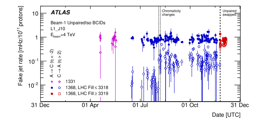
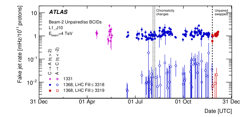
Figure 16: Rate of fake jets in the nominal RF buckets ($-2\,$ns $<t<0\,$ns) associated with beam-1 ($\eta<-2$) and beam-2 ($\eta>2$) are shown for the unpaired isolated bunches defined for beam-1 (a) and beam-2 (b). Each point corresponds to one LHC fill. Solid symbols represent jets with a timing consistent with the beam direction, while open symbols show jets with timing in the opposite direction. Events with jets at $4\,$ns $<t<6\,$ns are subtracted in order to correct for the pedestal. A vertex veto is applied to remove ghost collision contributions. The vertical lines indicate important changes in the beam conditions, as detailed in table 3.

Figure 16 shows the rate of fake jets at $|\eta|>2$ as a function of time, where contributions from beam-1 (beam-2) are expected at negative (positive) $\eta$. The contribution from the nominal RF bucket is enhanced by restricting the jet time window to $-2\,\textrm{ns}<t<0\,\textrm{ns}$ and subtracting the pedestal contribution, estimated from $4\,\textrm{ns}<t<6\,\textrm{ns}$ (see figure 15). Figure 16 also shows the rate of jets in the direction opposite to the unpaired bunch, which can be attributed to ghost-BIB. In figure 16 these ghost-BIB rates show a sudden jump in early August, when the LHC chromaticity change took place, consistent with the appearance of the opposite direction “banana” in figure 14. The opposite direction background in beam-1 unpaired bunch positions, shown in figure 16 remains at low level throughout the year with no evident jump in mid-August. A detailed discussion of these observations is deferred to section 9.2.

8.2 Non-collision backgrounds in colliding bunches

Fake jet rates can also be measured in the colliding bunches where they lead to events with balancing the transverse momentum of the fake jet, overlaid on top of minimum-bias interactions. Such events are recorded by triggers. In the following, the lowest unprescaled trigger available throughout 2012 with an $80\,$ threshold at L1 will be used together with an offline selection of $\MET>160\,$ and a requirement of a jet with $p_{\rm T}>120\,$ and $|\eta|<2.5$.

The missing transverse momentum is calculated from the vector sum of the measured muon momenta and reconstructed calorimeter-based objects (electrons, photons, taus, and jets), as well as calorimeter energy clusters within $|\eta|<4.9$ [24] that are not associated to any of these objects. Energy deposits reconstructed as tau leptons are calibrated at the jet energy scale.

Noise spikes are mostly suppressed by standard quality requirements at the data reconstruction stage, described in section 4.3. The remaining significant noise contributions are identified in the $\eta$–$\phi$ distribution of jets and the corresponding regions are masked in the offline analysis.

Multi-jet processes where a jet is mismeasured are efficiently suppressed by requiring a minimum azimuthal separation of $\Delta\phi(\textrm{jet},\MET)>0.5\,$rad between the missing transverse momentum direction and all jets with $p_{\rm T}>30\,$ and $|\eta|<4.5$.

The dominant Standard Model processes passing this selection are $Z\rightarrow\nu\nu$+jets and $W\rightarrow l\nu$+jets. Further processes involving top quarks and dibosons, that contribute to the total Standard Model expectation by less than approximately 10% over the whole $\MET$ spectrum, are neglected in this study. Figure 17 compares Monte Carlo (MC) simulations and recorded events in 2012 data, passing the selection described above. In the MC simulations the $Z\rightarrow\nu\nu$+jets and $W\rightarrow l\nu$+jets electroweak processes are generated using Sherpa 1.4.1 [25], including leading-order matrix elements for up to five partons in the final state and assuming massive $b$/$c$-quarks, with the CT10 [26] parton distribution functions. The Monte Carlo expectations are normalised to next-to-next-to-leading-order (NNLO) perturbative QCD predictions using DYNNLO [27, 28] and MSTW2008 NNLO parton distribution function set [29]. The generated events are interfaced with the GEANT4 [30] detector simulation.

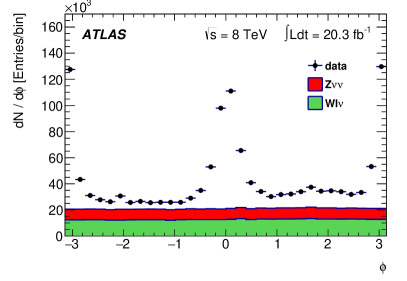
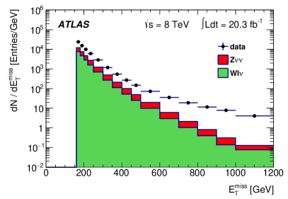
Figure 17: Distributions of the leading jet $\phi$ (a) and (b) in the events from colliding bunches triggered by the trigger with an offline requirement of $\MET>160\,$. Data is compared to the Standard Model expectation from the $Z\rightarrow\nu\nu$+jets and $W\rightarrow l\nu$+jets electroweak processes. Other $pp$ collision products, such as top and dibosons, that contribute to the total expectation by less than approximately 10% over the whole $\MET$ spectrum are not shown.

Approximately 1.4 million data events are selected from the full 2012 dataset, out of which more than half correspond to non-collision backgrounds. The azimuthal distribution of the leading jet, shown in figure 17, exhibits clear spikes at $\phi=0$ and $\pi$, that are characteristic for beam-induced backgrounds [1], on top of the uniform distribution from the $pp$ collision products described by the Monte Carlo simulation. Figure 17 shows that the spectrum of fake jets in the distribution is harder than the one expected from the electroweak processes.

The plots in figure 17 reveal that with a simple selection, based on jets and only, almost twice as many events were selected than predicted by Monte Carlo simulations. In the context of $pp$ collision data analyses, this illustrates how crucial it is to design an efficient jet cleaning strategy. In order to reduce this large NCB contribution to a sub-percent level, a suppression power of approximately $10^{3}$ is needed (see reference [1] for further discussion).

Fake jets due to noise or BIB muons have the common feature that there are usually no tracks connecting the measured calorimeter signal with the primary vertex. This is also true for fake jets induced by CRB, provided the path of the CRB-muon is not passing close to the IP. Furthermore, both noise and calorimeter deposits due to BIB muons often are contained in a single layer of the barrel calorimeter. These characteristics of NCB motivate use of the following quantities for the jet cleaning:

• Charged particle fraction, $f_{\textrm{ch}}$, which is the fraction of the total transverse momentum of a jet coming from tracks with $p_{\rm T}>500\,$.

• Maximum energy fraction in any calorimeter layer, $f_{\textrm{max}}$.

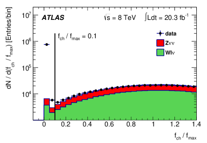
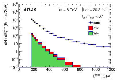
Figure 18: The distribution of the ratio $f_{\textrm{ch}}/f_{\textrm{max}}$ for leading jets in the events from colliding bunches triggered by the trigger with an offline requirement of $\MET>160\,$ (a). The value $f_{\textrm{ch}}/f_{\textrm{max}}=0.1$, used to separate NCB from $pp$ collision processes, is indicated by the black line. The distribution for the NCB events determined by the $f_{\textrm{ch}}/f_{\textrm{max}}<0.1$ selection (b). Data is compared to the Standard Model expectation from the $Z\rightarrow\nu\nu$+jets and $W\rightarrow l\nu$+jets electroweak processes. Other $pp$ collision products, such as top and dibosons, that contribute to the total expectation by less than approximately 10% over the whole $\MET$ spectrum are not shown.

The distribution of the ratio $f_{\textrm{ch}}/f_{\textrm{max}}$ for leading jets, shown in figure 18, suggests that $f_{\textrm{ch}}/f_{\textrm{max}}>0.1$ is an efficient cleaning selection. While for higher values the data are well described by the Monte Carlo simulation, NCB cause an excess at low values, which amounts to about two orders of magnitude with respect to the simulation. By requiring $f_{\textrm{ch}}/f_{\textrm{max}}<0.1$, a sample of fake jets can be extracted for which the Monte Carlo simulation predicts a 1% contamination from $pp$ collision processes. Figure 18 shows that the purity of BIB events becomes even higher with increasing .

Figure 19 shows the evolution of the NCB rate observed in the colliding bunches using this inverted cleaning selection. A gradual decrease of fake rates is observed in the early part of the year, possibly related to continued vacuum conditioning by beam scrubbing. The rates become stable after the June technical stop (TS2) where the fill pattern with 1368 colliding bunches was mostly used. The early drop is not observed in figure 16, but it should be noted that figure 19 requires much more energetic jets. The differences, therefore, could point at a different origin of the BIB generating the jets. As demonstrated in figure 14, the contribution from individual beams can be isolated at high $\eta$. Since the contribution from BIB in the selected fake jet sample dominates over CRB at low $\MET$ (see section 8.3), this allows studying the difference of BIB rates associated with the two beams. In figure 20 similar rates are observed in both beams after the April technical stop (TS1) while the beam-1 rate is significantly higher at the beginning of 2012 data-taking.

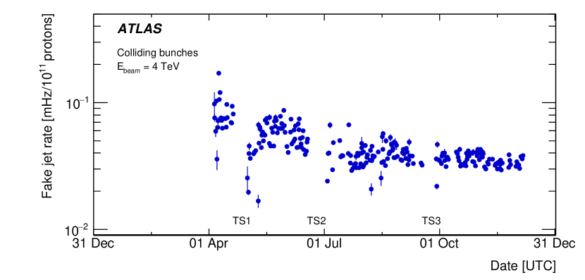
Figure 19: The rate of NCB in colliding bunches triggered by the trigger with an offline selection of $\MET>160\,$. The $\sim 1\%$ contamination of $pp$ collision products is not subtracted. Each point corresponds to one LHC fill. The technical stops are indicated in the plot.

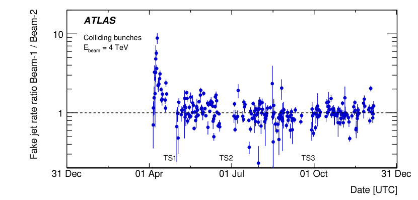
Figure 20: Evolution of the ratio of the NCB levels associated to beam-1 and beam-2 in the events triggered by the trigger with an offline selection of $\MET>160\,$ in colliding bunches. The beams are separated according to the leading jet $\eta$, where the beam-1 (beam-2) contribution is taken from $\eta<-1.2$ ($\eta>1.2$). Each point corresponds to one LHC fill. The technical stops are indicated in the plot.

8.3 Fake jets in cosmic-ray events

In analogy to BIB, CRB muons entering ATLAS can generate fake jets by radiative processes in the calorimeters. The rate and properties of such jets have been studied using two dedicated data-samples taken in November 2012 while the LHC machine was in cryogenics recovery, i.e. during which beams were not present in the LHC. The CRB data were recorded with all ATLAS detector sub-systems operational and a total live-time of 30.4 hours.

The fake jet properties are investigated in the data selected by a single-jet L1 trigger with a jet $p_{\rm T}$ threshold of 30 . An offline jet transverse momentum requirement of $p_{\rm T}>40\,$ ensured full trigger efficiency. The trigger was active in 3473 out of 3564 BCIDs and data rates quoted below are corrected for this 2.5% live-time inefficiency.

The rate of CRB muons decreases rapidly with energy [31]. Over most of the energy range bremsstrahlung is the most important radiative process that can result in a large local energy loss. The cross sections of all radiative processes increase slowly with muon energy. The bremsstrahlung spectrum follows roughly a $1/\nu$-dependence, where $\nu$ is the fraction of the muon energy transferred to the photon [32]. Most of the energy loss of muons is due to continuous processes and since they are effectively minimum ionising particles, they are expected to lose on average $\sim$40  when passing through the overburden from the surface to the ATLAS cavern. However the presence of the access shafts allows lower energy muons to reach ATLAS. Several samples of Monte Carlo simulated CRB muon events at the surface are therefore generated in different energy ranges, covering $50\,<E_{\mu}<100$ , and simulated with GEANT4. The samples are normalised to the differential CRB muon flux parametrised in reference [33].

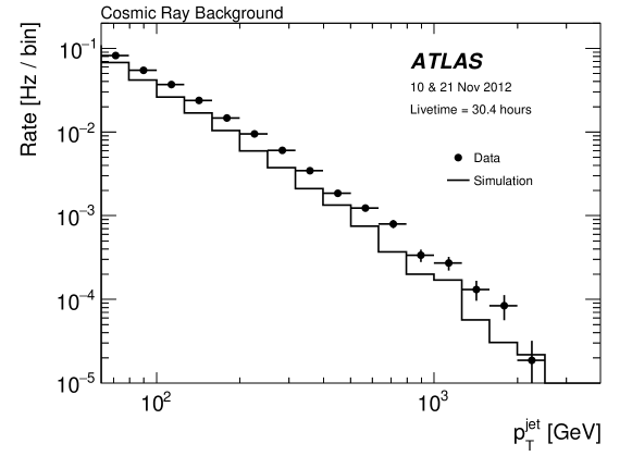
Figure 21: Distributions of the transverse momentum of the leading reconstructed jet in the selected events from the dedicated CRB data-taking. Data are compared to the CRB-muon Monte Carlo simulation.

The distributions of the apparent transverse momentum, calculated with respect to the nominal beamline, are shown in figure 21 for the leading reconstructed jets in selected events. The total rates in data and Monte Carlo agree to within $\sim$50%. While such a discrepancy would be considered large for simulation of $pp$-collisions, it is reasonably good agreement for this kind of simulation. The uncertainties in the shape and normalisation of the parametrisation of the muon flux at the surface are about 10%. More significant uncertainties are related to the muon transport through the overburden, i.e. the exact density and composition of the $\sim$60 m thick soil above the experiment. The principal message of figure 21 is, that the simulations describe well the spectrum of the CRB related fake jets up to the highest apparent $p_{\rm T}$-values.

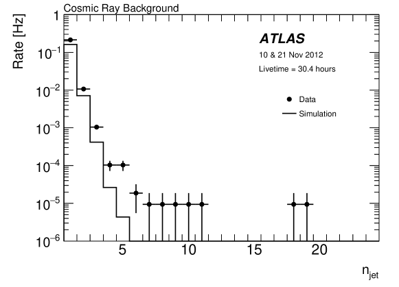
Figure 22: Distribution of the multiplicity of jets with $p_{\rm T}>10\,$ and $|\eta|<4.5$ in events containing at least one jet with $p_{\rm T}>40\,$, using the dedicated CRB data, compared to the CRB-muon Monte Carlo simulation.

Figure 22 shows the distribution of jet multiplicities ($n_{\rm jet}$) for selected events containing at least one jet with $p_{\rm T}>40\,$. The data and Monte Carlo distributions agree to within $\sim$ 30% for $n_{\rm jet}<3$, indicating that the Monte Carlo simulation of single CRB muons provides a reasonable representation of the data at low jet multiplicities. The deviation of the absolute normalisation is related to that observed in figure 21. For jet multiplicities above two, however, the number of selected data events significantly exceeds the Monte Carlo expectations. This is to be expected due to the presence of multiple-muon events in the data generated by extensive air showers [34, 35, 36], which are not modelled by the Monte Carlo generator.

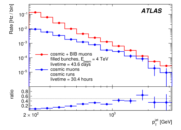
Figure 23: Distributions of the leading jet transverse momentum in the fake jet samples obtained from the colliding bunches and the dedicated CRB data. The ratio indicates the fraction of CRB in the NCB sample. Only the fills with 1368 colliding bunches are taken in the former case.

The fake jet rates from the dedicated CRB data are also directly compared to the rates of NCB obtained from the colliding bunches in section 8.2. For this, additional selection criteria are applied in the CRB data in order to ensure consistency of the fiducial volumes of the two samples. Therefore, the CRB data are further restricted to contain only leading jets in the tracker acceptance $|\eta|<2.5$ that pass the inverted cleaning selection $f_{\textrm{ch}}/f_{\textrm{max}}<0.1$ used to select the NCB events from the colliding bunches. Furthermore, the same kinematic and topological selection as in section 8.2 is imposed. A comparison of the rates is shown in figure 23 for jet $p_{\rm T}>200\,$. The higher jet $p_{\rm T}$ threshold is chosen in order to avoid turn-on effects caused by the $\MET$ selection in the CRB events where both the muon and the induced fake jet are reconstructed in such a way that the two objects weigh against each other in the $\MET$ calculation. The NCB rate from the colliding bunches is corrected for the live-time of the 2012 data-taking with 1368 colliding bunches. As in the case of the rate from the CRB data, the rate is scaled up such that it corresponds to all 3564 BCIDs being filled with a nominal bunch. As stated in section 8.2, the noise contribution in the NCB rate is suppressed, i.e. the dominant components are fake jets from BIB and CRB. The plot shows that the fake jet rate from BIB is 10 times higher than from CRB at $p_{\rm T}\sim 200\,$ but the difference gradually decreases with increasing $p_{\rm T}$. Beyond $p_{\rm T}\sim 1\,$, the CRB fake jets contribute at a similar level as BIB jets, although the CRB dataset becomes statistically limited there, preventing a firm statement.

9 BIB from ghost charge

Although the intensity of ghost bunches is very low, they still can produce BIB, just like nominal bunches. When other contributions are sufficiently suppressed by suitable selection, those small BIB signals can be seen both by the BCM and as fake jets. This section will describe several observations made on those ghost-BIB signals.

9.1 BCM background from ghost charge

In section 7 it was shown that the L1_BCM_AC_CA background for unpaired bunches is dominated by beam-gas. If this were true also for ghost bunches, then the BIB rate from them should scale with intensity.

It was already alluded that the small early peaks in downstream modules, seen in figure 5, can be attributed to BIB from ghost bunches in the opposite beam. However, the relative heights of those peaks with respect to the peaks from the unpaired bunches appear too high with respect to typical injected ghost bunch intensities, which according to figure 9 are at least a factor $10^{3}$ lower than those of unpaired bunches.

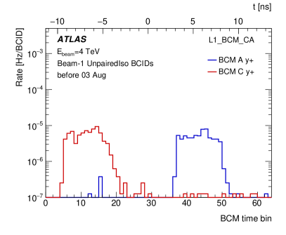
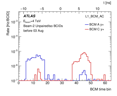
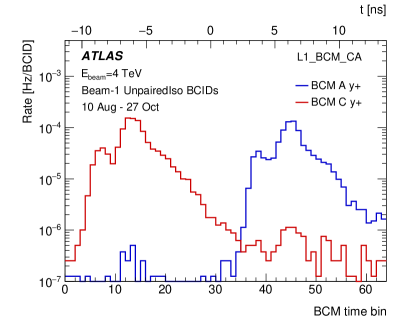
Figure 24: Hits in the individual BCM stations in the events triggered by L1_BCM_CA_UNPAIRED_ISO for beam-1 BCIDs (a, c) and L1_BCM_AC_UNPAIRED_ISO for beam-2 BCIDs (b, d), i.e. in all cases opposite to the unpaired bunch direction. The plots (a) and (b) show data before 3 August while (c) and (d) show data from 10 August until the onset of the BCM noise. Only fills with 1368 colliding bunches are considered.

The ghost-BIB signals can be extracted from figure 5 by considering only the events which have a BCM background trigger in the direction opposite to the unpaired bunch. The rates after this selection are shown in figure 24 for both beams. The data are divided into periods before and after the LHC chromaticity changes.

In the plots corresponding to fills before the chromaticity changes the opposite direction signals are distributed almost uniformly in the trigger window, with only a slight hint of a peak structure. This suggests that most of the rate is due to random coincidences of the pedestal. However, from 10 August onwards, clear peaks are seen, especially in events triggered by L1_BCM_CA, i.e. in beam-2 direction. The early and in-time peaks have very similar size and shape, indicating that the peaks are due to genuine background tracks and not accidental coincidences of noise or afterglow_pp. Furthermore, sub-peaks can be distinguished, 2.5 ns (6 bins) before the main peak. This corresponds to the spacing of the RF buckets in the LHC, and further confirms that these peaks are related to ghost bunches.

After mid-August the ghost-BIB is much larger for beam 2, i.e. in beam 1 unpaired positions. This seems to be in conflict with figure 8, which indicates that the intensity of injected ghost bunches (colliding with unpaired bunches of beam 2) is higher in beam 1.

The main peak seen in figure 24 after 10 August is located in the bucket paired with the unpaired bunch in beam-1, i.e. it should be probed by the collision rate of figure 8. The BCID-dependence of the rate, obtained by this collision probing, is consistent with the product of the bunch intensity data from the LDM for fill 3005 (26 August), shown in figure 9(b). Thus both the collision probing and LDM show more ghost charge in beam-1, while the BIB rates in the direction opposite to the unpaired bunches indicate more background from beam-2 ghost bunches.

This apparent paradox can be resolved by postulating that the ghost-BIB is dominated by cleaning debris and not by beam-gas interactions. Under this assumption the asymmetry of the LHC, with respect to beam cleaning insertions, plays an important role in explaining the observations. The momentum cleaning, located in IR3, is only two octants away from ATLAS along beam-2, but 6 octants along beam-1. In addition beam-1 has to pass both IR5 (CMS) and IR7 with its very tight betatron collimation. Thus, debris from momentum cleaning in IR3 is much more likely to make it to ATLAS in beam-2 than in beam-1.

Since the IR3 collimators are at very relaxed settings with respect to the normal momentum spread [37], protons contained in a normal bunch will not be intercepted in IR3. Protons de-bunched in the LHC itself, i.e. having escaped their original buckets and drifting in the ring can develop large enough a momentum offset to reach IR3 collimator jaws. As explained in section 3 this de-bunched ghost charge is rather uniformly distributed in the entire ring and therefore the contribution from IR3 debris to the BIB is roughly the same for all RF buckets, including those filled with a nominal bunch. A nominal bunch has at least 3 orders of magnitude higher intensity than a ghost bunch and since the beam-gas rate is proportional to intensity, the role of IR3 debris for nominal bunches is negligible compared to close-by beam-gas scattering. For the low-intensity ghost bunches, however, the small component of IR3 debris can constitute the dominant background.

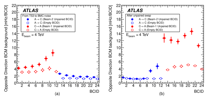
Figure 25: L1_BCM_AC (L1_BCM_CA) trigger rates per BCID from ghost-BIB before and after the swap of the unpaired trains. The BCM noise period has been excluded. From each fill the first five hours of stable beams have been considered. Fills shorter than that are not included. The mean values correspond to the average of several fills and the error bars indicate the RMS of the mean.

The swapping of the unpaired trains at the end of 2012 $pp$-operation provides a good means to test this hypothesis. The systematic tendency for higher intensity in trailing than heading injected ghost bunches implies that after the swap the intensity of injected beam-2 ghost bunches (L1_BCM_CA triggers) in beam-1 unpaired locations should be higher than before the swap. A comparison of per-BCID rates between mid-August and the onset of the BCM noise, and after the swap of unpaired trains is shown in figure 25. The data clearly indicate that even when the beam-1 train is first, there is more BIB from injected beam-2 ghost bunches than from beam-1, consistent with figure 24. After the swap of the unpaired trains the BIB from injected beam-1 ghost bunches is very low, while there is a large increase for beam-2, as expected.

Figure 26 shows the BCM background rates due to ghost bunches for all 2012 fills with 1368 colliding bunches. A sudden increase of background from beam-2 ghosts is seen, coincident with the chromaticity changes in early August [38], while no rise is seen in the beam-1 direction. At the same time, the fill-to-fill scatter increases significantly. Since chromaticity settings might affect how tight the momentum cleaning in IR3 is, this observation further supports the interpretation that the excess background, attributed to ghost bunches, originates from IR3.

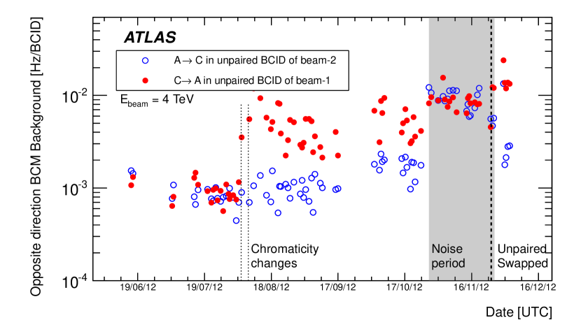
Figure 26: Evolution of the opposite direction BCM background for both beams throughout 2012. Only ghost bunches in BCIDs with an unpaired bunch in the other beam are considered. The plot is restricted to fills with the 1368 colliding bunches pattern, which all have the same configuration of 6+6 unpaired bunches. Only the first five hours of stable beams are considered and shorter fills are ignored. Data in the period between 27 October and 26 November suffer from the BCM noise and should be ignored.

9.2 Fake jets from ghost bunches

The rates in the C$\rightarrow$A direction in figure 26 have a clear similarity to the corresponding fake jet rates due to BIB muons in the C$\rightarrow$A direction, observed in figure 16. This strongly suggests that the jump in early August, which manifests itself in both background observables, has the same origin.

The fake jet rates due to the ghost bunch in the colliding bucket can be extracted from the events without any vertex by selecting jets with time $-2\,\textrm{ns}<t<0\,\textrm{ns}$ at $\eta<-2$ and $\eta>2$ for beam-1 and beam-2, respectively.

Figure 27 shows the rates obtained with this selection and averaged over fills before and after swapping of the unpaired train. The similarity with figure 25 provides further evidence that the sources of the background are the same or at least strongly correlated.

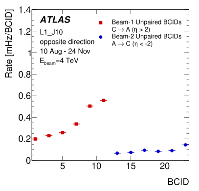
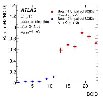
Figure 27: Rate of fake jets associated with ghost-BIB from the opposite beam after mid-August (a) and after the swap of the unpaired trains (b).

The timing distributions for fake jets in the direction of the unpaired bunches at $|\eta|>2$ are shown in figure 15 for data before early August and those after mid-August. Two peaks can be observed in figure 15 with the larger one at $t\sim 0$, corresponding to BIB from the unpaired bunch. The large peak has equal size for both beams, which follows naturally from the very similar pressure distributions on both sides, if the fake jets are entirely due to beam-gas events. The beam cleaning, however, is asymmetric with respect to the two beams, so figure 15 implies that either the beam-halo contribution to fake jets from unpaired bunches is negligible or halo losses of unpaired bunches are also very similar on the two sides.

In figure 15 as well a prominent peak from the unpaired bunches is observed at $t\sim 0$. Its size is the same as in figure 15, which implies that there is no change in the BIB from unpaired bunches. Unlike in figure 15, several smaller peaks are observed in figure 15, especially for beam-2. These peaks reflect the 2.5 ns time-structure of the LHC RF, which is consistent with them being due to ghost charge produced by de-bunching in the LHC. The level of these peaks, however, is only a factor 20–50 below the main peak, which is much less than the intensity difference (at least 3 orders of magnitude) between nominal and ghost bunches. This observation, that ghost bunches produce more background per unit intensity than nominal ones, provides further evidence that their losses are dominated by beam cleaning and not beam-gas interactions.

Figure 28 shows the timing distribution of fake jets in the direction opposite to the unpaired bunch, i.e. corresponding to ghost-BIB from the other beam. Like in figure 15, smaller peaks reflect the RF structure and indicate that the ghost charge is distributed among all buckets. It should be noted that there is no central peak in the $A\rightarrow C$ direction, just an almost uniform pedestal. This is consistent with the assumption that there is negligible fake jet production due to beam-1 ghost bunches and the observed rate is due to the smeared-out incoming beam-2 contribution where individual buckets cannot be resolved. In the $C\rightarrow A$ direction, the side-peaks are clearly visible, but the absolute level is similar to the other direction. The reason is that in both directions the rate is dominated by beam-2 ghost-BIB, but only in the $C\rightarrow A$ direction, i.e. downstream, is the time-spread small enough to resolve individual buckets (see figure 14). A comparison of the pedestals, i.e. the rates for $|t|>4$ ns, reveals that their levels are almost identical in figures 15 and 28. This is consistent with the pedestal being dominated by losses of the debunched ghost charge, which mostly are smeared out in time.

In figure 28 the peak in the nominal position, at $t\sim 0$, is larger than the other peaks. While it is established that the injectors generate more intense injected ghost bunches in the nominal RF buckets, it is also assumed that those bunches would not be sufficiently off-momentum to reach IR3 cleaning. It is possible, however, that those low-intensity injected ghost bunches develop larger off-momentum tails than nominal ones. Another observation that can be made in figure 28 is that the side-peaks in the beam-2 (C$\rightarrow$A) direction are higher for earlier arrival, $t<0$, than for $t>0$. This might be related to a preferred direction of de-bunching from the injected ghost bunch in the $t=0$ bucket: de-bunching is predominantly due to energy loss, as a result of which the particle moves to a slightly smaller radius and arrives earlier on subsequent turns.

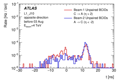
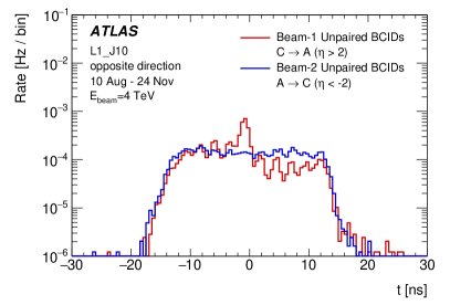
Figure 28: Jet times in the direction opposite to the unpaired bunch for fake jets at $|\eta|>2$ without a reconstructed vertex for the period before 3 August (a) and between 10 August and the swap of the unpaired bunches (b). Only fills with 1368 colliding bunches are considered. The plots are normalised by the live-time, the rate is averaged over the six unpaired BCIDs per beam and the bin width is 0.5 ns.

These observations of fake jets caused by de-bunched ghost charge, distributed all around the ring, imply that some specific physics analyses, in particular searches for long-lived heavy particles, must consider the presence of fake jet background due to BIB in all RF buckets. An example of an analysis, properly accounting for the possible presence of such backgrounds, can be found in reference [14].

9.3 Ghost bunches in the abort gap

It was argued before that the de-bunched ghost charge, the source of beam-2 ghost-BIB, is spread uniformly over the ring. This implies that the effect should be visible also in BCIDs, which are not paired with an unpaired bunch in the other beam. An observation of the beam-2 excess in such BCIDs would also exclude any accidental coincidences involving the unpaired bunch. Such an excess in the beam-2 (C$\rightarrow$A) direction can, indeed, be seen in the rates shown for empty bunches in figure 25, but the cleanest possible sample of empty bunches can be found in the abort gap.

Figure 29 shows the background rates due to ghost-BIB as a function of BCID. It is evident that prior to the chromaticity changes both beams produce very similar levels of BIB, dominated by accidental background-like coincidences from afterglow_pp or noise. The gently falling slope is explained by the decreasing afterglow_pp following colliding trains before the abort gap. The situation is entirely different after mid-August: while the same smooth slope is observed for beam-1, the BIB from beam-2 reveals a periodic structure of humps. As indicated by the small error bars – which include the effect of fill-to-fill differences – the pattern of the humps is the same for all fills.

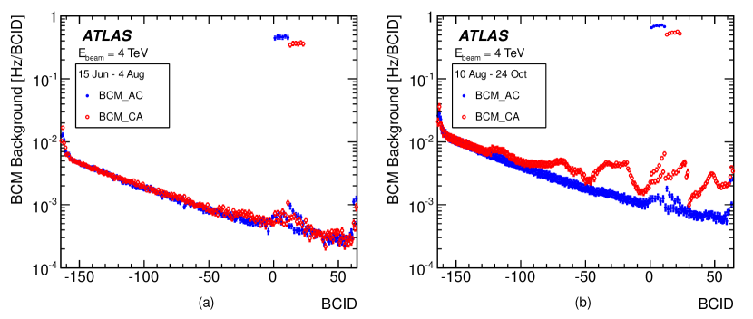
Figure 29: L1_BCM_AC (beam-1) and L1_BCM_CA (beam-2) background rates in the abort gap region. The points correspond to the average over all fills with the 1368 colliding bunch pattern, using the first five hours of stable beams and the error bars show the RMS of this average, thus reflecting any fill-to-fill variation. Fills shorter than five hours are not considered. Data shown are averages over periods before (a) and after (b) the LHC chromaticity changes. For plotting, the BCIDs in the abort gap have been re-mapped to negative values by BCID = BCID_true - 3564. The high rates just above BCID=0 correspond to the unpaired bunches.

The presence of the humps in the fake jet rates cannot be verified since the fake jet analysis is based on recorded data and, due to the lack of a dedicated jet trigger in the abort gap, suitable data were not recorded in 2012.

An obvious question is if, and how, the humps evolve during a fill. Since the rate is very low, there is not enough statistics to study the time-dependence for a single BCID in a given fill. Only an integration over longer time and many fills provides enough data to clearly see the structures.

An additional complication is that the random background from afterglow_pp masks the humps, especially at the start of the abort gap and early in the fill when the luminosity is high. This contribution, however, can be subtracted if it is assumed that the rate is fully random and caused by noise and afterglow_pp only. For this, the luminosity data have been used taking the product of the BCM-TORx rates of both sides as an estimate for the random pedestal coincidences. Window-width and efficiency corrections are not performed, instead the data are matched in the region of BCID 3400 to 3425 (shown as $-164$ to $-139$ in figure 29). The method reproduces very well the hump-free slope for beam-1 which gives confidence that it is a valid estimate of the random background.

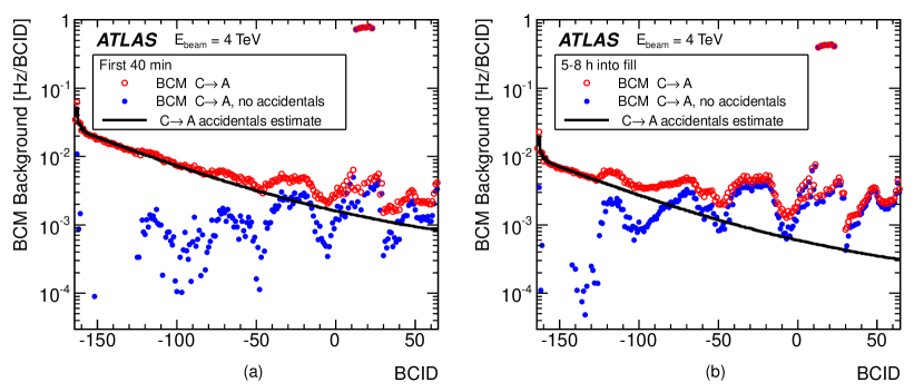
Figure 30: L1_BCM_CA (beam-2) background rates in the abort gap region for two time-ranges during stable beams. The open circles show the total data. The line represents an estimate of the random coincidence rate, as explained in the text. The solid circles show the data with the random rate subtracted. The fills used for plot (b) are a subset of those used for plot (a). Only fills between mid-August and the onset of the BCM noise have been considered. For plotting, the BCIDs in the abort gap have been re-mapped to negative values by BCID = BCID_true - 3564.

Figure 30 shows a comparison of beam-2 ghost-BIB for the first 40 minutes of STABLE BEAMS and for the time between 5–8 h into STABLE BEAMS mode, using all available fills (of which there were more for the 40 minutes plot). The rate after random background subtraction reveals that the humps remain in the same position and their magnitude shows only a slight sign of increase with time. The decrease of the random background in the course of the fill causes the humps to show up more clearly.

In the second half of 2012 $pp$ operation, an abort-gap cleaning method [39] was exercised in several fills. The principle of abort gap cleaning is that excitations are introduced by the transverse damper system of the LHC. Figure 31 shows how BIB rates in different BCID-ranges of the abort-gap react to the cleaning in fill 3067. The cleaning was switched on and off several times during the fill. The BCID ranges are shown in figure 31, which gives per-BCID rates averaged over the periods indicated in figure 31. The solid black curve in figure 31 shows the estimated contribution from random coincidences. This has been subtracted in figure 31.

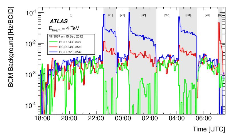
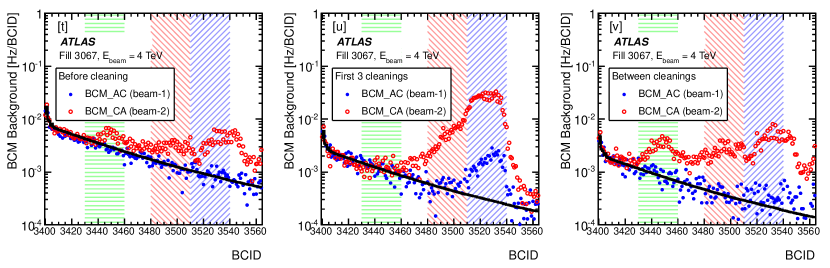
Figure 31: Time development (a) of the beam-2 hump sizes in the abort gap in a fill where abort gap cleaning was repeatedly active (shaded areas). The random coincidence background has been subtracted. The BCID-ranges corresponding to the three histograms are indicated in figure (b) where the background in the abort gap for both beams is shown. The data labelled [u] and [v] have been averaged over the periods indicated in (a), i.e. [u] shows an average over [u1]-[u3] of figure (a), and correspondingly for [v]. The hatched areas in figure (b) correspond to the three histograms, i.e. BCID-ranges, shown in figure (a). The curve indicates the estimated random coincidence background.

Figures 31 and 31 show that as soon as the cleaning is switched on a large hump develops in the latter part of the abort gap while the hump in the early part is strongly suppressed. This suggest that the gap is filling up from the “right” (in figure 31), i.e. off-momentum particles tend to move faster and arrive earlier. When the cleaning is switched off, a reduction of BIB rates is seen for all BCID ranges shown in figure 31, but only in the first bin (1 luminosity block, i.e. typically 60 s) following the cleaning. Thereafter the BIB rates return to their pre-cleaning levels. This indicates that the time-scale to repopulate the abort gap is of the order of one minute, which is in good agreement with the estimate presented in reference [17].

The last cleaning period seen in figure 31 shows a different behaviour. It appears that the excitation affects a different BCID range. Unfortunately the period is too short to obtain enough statistics in order to include it in figure 31.

The cleaning was active for both beams simultaneously. In figure 31 also the BIB rates from beam-1 are shown and it can be seen that, when the cleaning is active, losses are significant enough for a visible hump to develop also for beam-1.

Finally, it should be emphasised that figures 29 – 31 show a quantity that depends on the loss rate of protons in the abort gap, not the abort gap population itself. This is also the reason why the humps increase when the cleaning is switched on.

10 Backgrounds in special fills

During 2012 operation three fills with special conditions exhibited backgrounds which motivated detailed studies. The first was a normal physics fill with exceptionally high background in beam-1. Studies of this fill provide insights into the reconditioning of the vacuum following an accidental local gas release.

The second case is a dedicated high-$\beta^{*}$ fill with very intense periodic beam cleaning. The low beam intensity and luminosity of this fill resulted in strongly reduced beam-gas rates and afterglow. At the same time the losses in the beam cleaning insertions were temporarily very high. In these particular conditions the correlation between beam cleaning and backgrounds in ATLAS could be studied in detail. The results obtained provide interesting insights and suggest similar studies for the normal optics in LHC Run-2.

The third fill to be discussed is a test with a 25 ns bunch spacing, performed at the end of 2012 proton operation. The backgrounds observed during this short test establish a reference point for LHC Run-2, in which a 25 ns bunch spacing is the baseline.

10.1 High background fill

In LHC fill 3252 abnormally high BIB levels from beam-1 were observed in ATLAS for the first 90 minutes of stable beams. During this time the background gradually decreased from about a 40-fold excess back to almost the normal level. At the same time no excess was seen in beam-2 backgrounds.

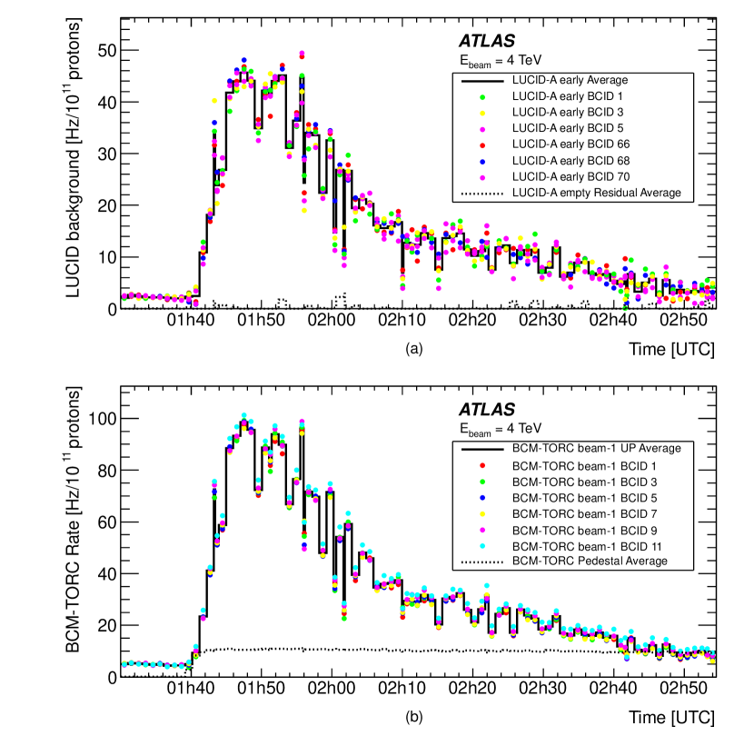
Figure 32: Beam-1 background as a function of time at the start of stable beams in LHC fill 3252, as seen by LUCID (a) and BCM (b). The lines show the averages over BCIDs, while the symbols show individual BCIDs. The bins correspond to ATLAS luminosity blocks, the widths of which varied from 10 s to the nominal 60 s. The dotted histograms are normalised per BCID, since there is no applicable bunch intensity.

The large background was seen by all inner detectors which were capable of resolving it from the debris from $pp$ collisions. Due to their $\sim$40 $\upmu{\rm s}$ integration time, the BLMs close to ATLAS were all dominated by $pp$ collision products and unable to resolve an excess of this size. Monitors in the cleaning insertions showed no structure with similar magnitude and temporal behaviour as the observed background, neither did vacuum gauges in IR1.

Figure 32 shows the detailed time-structure of the background, extracted from the single-sided luminosity data of BCM and using the incoming bunch signal of LUCID, as described in section 4.2. The LUCID method allows for monitoring of the background associated with the first three unpaired bunches of beam-1, and the first three paired bunches of the first train, i.e. bunches in BCIDs 66, 68 and 70. For all other bunches the LUCID signal overlaps with the overwhelming luminosity signal from bunch-bunch or bunch-ghost collisions.

At the A-side of LUCID the background signal from the first colliding bunches appears in BCIDs 61, 63 and 65. The pedestal level for these was estimated as an average over the empty BCIDs 57, 58 and 59. For the first unpaired bunches, the background signal appears in BCIDs 3559, 3561 and 3563, for which the pedestal is evaluated from BCIDs 3556–3558. In both cases the pedestal was found to be about three times larger than the background signal. However, since the pedestal is dominated by afterglow from trains several $\upmu{\rm s}$ earlier, it is very constant and could be subtracted in order to extract the signal. Thereafter the remaining signal is normalised by the bunch intensity. In order to estimate the uncertainty introduced by this method, the subtraction was applied also on BCIDs 60, 62 and 64, where no signal is expected. The result is shown by the dotted line in the upper plot of figure 32. The level, consistent with 0, indicates that contributions other than the beam background are efficiently removed by the pedestal subtraction.

With the BCM-TORx rates the unpaired bunches can be monitored but the rates include a contribution from ghost collisions. As shown in figure 3, the unpaired bunch signals are on top of a smoothly dropping background, which is removed by subtracting the rate in the preceding BCID. This pedestal estimate is indicated by the dotted line in the lower plot of figure 32. The remaining beam background signal is normalised by the bunch intensity.

The data from the two independent detectors exhibit a similar spiky time structure, which is clearly beyond statistical fluctuation. All bunches follow the same structure.

The origin of the high background could be attributed to an incident a few hours earlier: a quench of the inner triplet on side A of ATLAS had warmed up the beam-pipe and desorbed some gas from the cold bore. This event resulted in a pressure surge at vacuum gauges on the IP-side of the triplet ($p22$) and a slower increase in the gauge on the other side ($p58$), indicating that gas was distributed throughout the entire triplet length and certainly part of it was absorbed on the beam screen.

The inner triplet and its beam-screen are exposed to a significant heat-load from $pp$ collision debris, thus, at the beginning of the next fill, the beam-screen was scrubbed by the secondaries created in the collisions. This led to a pressure increase within the triplet, but since the beam pipe was now cold again, there was sufficient cryo-pumping that the gas did not diffuse to the gauges. Therefore, normal pressure levels were reported, while the actual pressure within the triplet must have been significantly above normal.

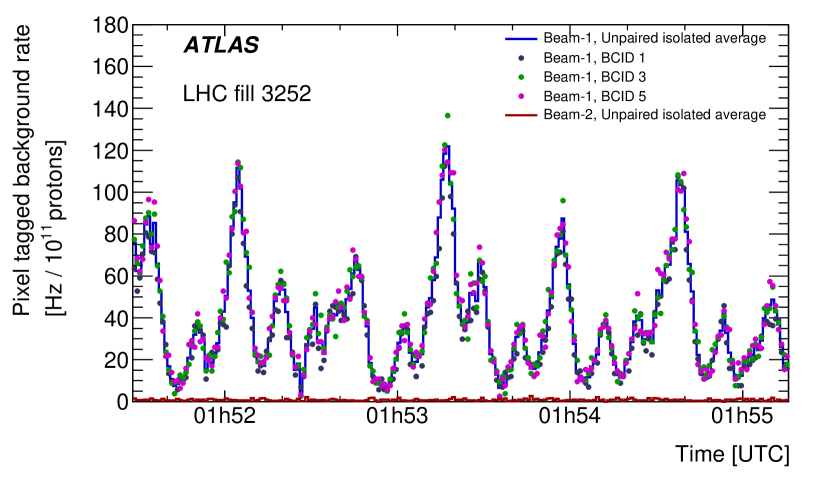
Figure 33: Background rate measured with the Pixel tagging method over 4 minutes during the period of highest rate. For beam-1 the average and the three unpaired isolated BCIDs are shown separately. For beam-2, with normal background, only the average is shown.

A third method to observe the background is provided by the Pixel detector using the background tagging tool developed in reference [1] and described in section 4.4. Unlike the luminosity data of BCM and LUCID, used for figure 32, the Pixel-tagged events are not sensitive to afterglow. The overall shape of beam-1 background seen by this method is perfectly consistent with figure 32, but since the tagged events have exact time-stamps, it is possible to significantly improve the time resolution. Figure 33 shows the time-dependence of the background over four minutes close to the maximum and a clear substructure is resolved. All unpaired isolated BCIDs exhibit a consistent periodic fluctuation with a frequency of the order of 0.1 Hz and significant amplitude. The temperature of the beam-screen is actively controlled and, indeed, the frequency of the background oscillations is very similar to the temperature fluctuations measured at the inlet of the beam screen cooling loop, suggesting that the rate of outgasing is strongly coupled to the beam screen temperature.

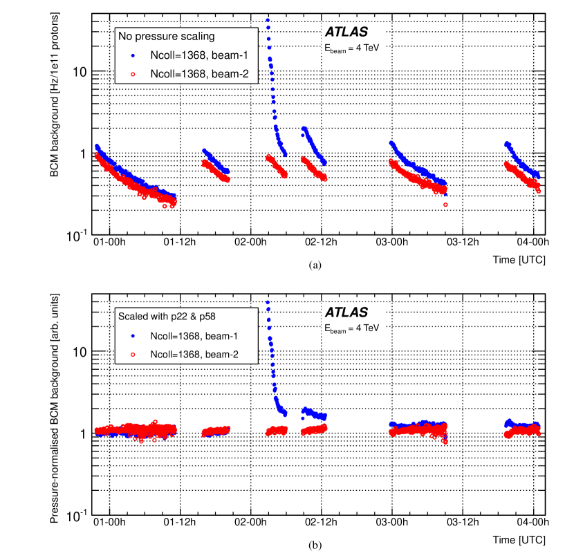
Figure 34: BCM_AC (beam-1) and BCM_CA (beam-2) backgrounds in the high-background fill and a few fills before and after. Unlike the luminosity data in figure 32, these triggers have negligible background contamination, but suffer from a time-resolution of only 300 s. Rates are shown before (a) and after (b) normalisation with the residual pressure. The high-background fill, 3252, is seen as the large excess in the middle of the plots.

In figure 34(b) the pressure scaling, derived in section 7.1, is applied to the rates, but has no reducing effect on the excess. This indicates that the additional background originates from a source that has no correlation with the pressure at 22 m. The scaling also reveals that even the next fills are affected, indicating that the scrubbing of the contaminated beam screen continues into several subsequent fills. In fact a close examination of figure 7(b) reveals that the scrubbing continues for about one week until the level of beam-1 background has dropped to the same level as of beam-2. This observation, made in figure 7, demonstrates that the pressure scaling significantly increases the sensitivity to any backgrounds not correlated with the 22 m pressure. This enables the detection of much smaller additional effects than without the pressure scaling.

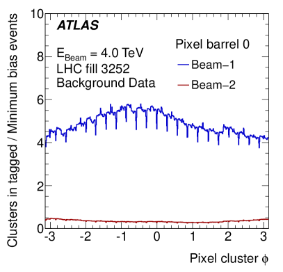
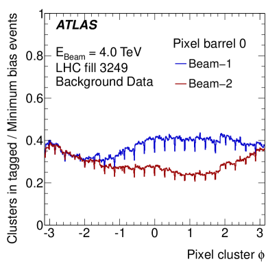
Figure 35: Azimuthal distribution of clusters in events tagged as background during the high-background phase in fill 3252 (a) and during the normal background fill 3249 (b). Rates have been normalised by minimum-bias events in the same fill to compensate for inefficiencies and overlaps of individual modules. Taking into account the very different vertical scale on the two plots – the histograms for beam-2 are in fact almost identical in the two fills. The small dips reflect a residual effect of the module overlaps which have different effects for tracks from the IP and from upstream BIB events.

The Pixel-based background tagger can be used to extract a detailed azimuthal dependence of the background in order to compare it with that of a normal fill. Efficiency differences of individual Pixel modules lead to a rather non-uniform azimuthal distribution of cluster rates even for minimum-bias events, which produce secondaries uniformly in $\phi$. In order to compensate for this and extract the azimuthal asymmetry of the BIB, the rates of clusters in events tagged as BIB have been normalised by the cluster rates of minimum bias events in the same fill. The results for the innermost layer of the Pixel detector are shown in figure 35. The very high rate of beam-1 background in fill 3252 is again illustrated by the difference of the level of beam-1 and beam-2 backgrounds seen in figure 35. The more interesting aspect, however, is that the azimuthal distribution is different from that seen in figure 35, which represents a normal fill. This indicates that the source distribution along the $z$-axis must be different in the two cases such that the secondaries traverse different magnet configurations. As argued before, in the high-background fill the beam-gas events must be localised in the inner triplet. In section 7 it is established that the background seen by the BCM correlates with the pressure at 22 m, i.e. the IP-end of the triplet, but this does not exclude the possibility of contributions from more distant locations, as long as they also correlate with the 22 m pressure. It is worth noting that the integral of the beam-1 histogram in figure 35 is found to be 29 % larger than that of beam-2. This difference is consistent with the 28 % found in sections 6 and 7 for the beam-1/beam-2 ratio of the BCM backgrounds. This agreement, and the observation of a different azimuthal distribution, support the assumption formulated at the end of section 7 that the background of beam-1 has either an additional contribution or originates from a different pressure distribution than that of beam-2.

10.2 Background in high-$\beta^{*}$ fills

LHC fill 3216, with $\beta^{*}$=1000 m, had a very low interaction rate, of the order of 0.005 $pp$ collisions per bunch crossing, and a sparse bunch pattern with only three nominal intensity bunches per beam, two colliding in BCIDs 101 and 1886 and one unpaired in BCID 901 and 992 for beam-1 and beam-2, respectively. Because the forward detectors, ALFA [40] and TOTEM [41, 42], approached the beam with their roman pots to a distance of only 3.0 nominal $\sigma$, the collimators in IR7 were temporarily moved as close as 2.0 nominal $\sigma$ in order to clean the immediate surroundings of the beam core. Around the same time IR3 collimators were closed to 5.9 $\sigma$ while TCTs in IR1 and IR5 were retracted to 17 $\sigma$ throughout the fill. These and other collimator settings are summarised in table 1. This tight cleaning resulted in very large beam losses over short durations of time. Against the very low luminosity background, these loss-spikes provided a particularly clean environment to study the relationship between proton losses at the primary collimators and background seen in ATLAS. It has to be emphasised, however, that the LHC optics was very different from nominal so these studies provide interesting insights, but do not allow conclusions for normal operating conditions.

Unfortunately, the time-resolution of 300 s, at which the per-BCID L1_BCM_AC_CA rates were recorded in 2012, is too coarse with respect to the duration of the loss peaks during cleaning. The very low luminosity and sparse bunch pattern, however, resulted in negligible afterglow, allowing the use of BCM luminosity data from one side of the detector only. For paired bunches this method suffers from the rate due to luminosity which, although very low, prevents from seeing small background spikes. For the unpaired bunch the sensitivity to background is about an order of magnitude better.

An even cleaner background measurement was obtained from the LUCID detector, using the signal of the incoming beam in the upstream detector, as described in section 4.2. As will be seen, a comparison between the two detectors is very useful, since in some cases it confirms real background while in others it uncovers mechanisms that result in wrong association of spikes to bunches.

Figure 36: Background seen by BCM (a, b) and LUCID (c, d) in the high-$\beta^{*}$ LHC fill 3216 in the paired (101, 1886) and unpaired (901, 992) bunches. Plots (a) and (c) show the hit rates from beam-1, while plots (b) and (d) show those from beam-2. Plots (e) and (f) give the corresponding bunch intensity loss rates for beam-1 and beam-2, respectively.

Figures 36(a–d) shows the observed beam-1 and beam-2 backgrounds as seen by BCM and LUCID while figures 36(e–f) indicate the loss in beam intensities. It can be seen that, especially in beam-2, large backgrounds are observed already at 20:15 UTC, about 10 minutes before any appreciable beam intensity loss is seen. A detailed analysis of BLM readings in the cleaning insertions, summarised in figure 37 together with the relevant collimator positions, reveals that the observed intensity losses are caused by IR7 collimators closing between 20:30 and 20:40 UTC (figure 37(c–d)). Collimators in IR3 (figure 37(a–b)), however, close already at 20:15 UTC and while they cause no visible intensity loss in figure 36(e) or (f) their movement and local losses seen in IR3 BLMs correlate perfectly with beam-2 background increase seen in ATLAS (figure 36(b) and (d)). This leads to the interpretation that ATLAS backgrounds from beam-2 are much more sensitive to losses in IR3 than those in IR7. This is not too surprising given that, for beam-2, IR3 is only two octants away from ATLAS.

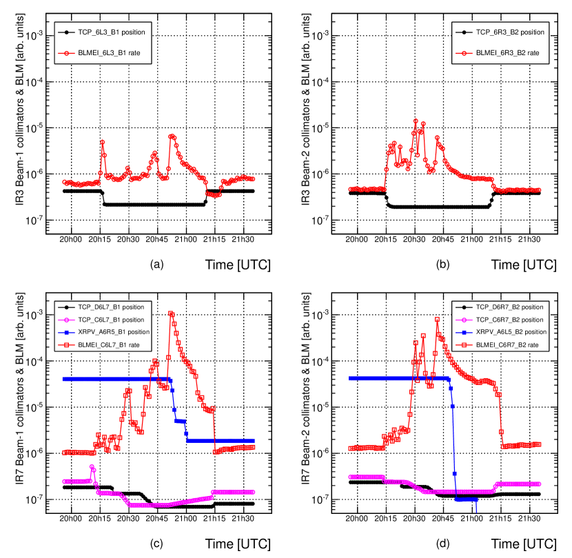
Figure 37: Loss rates (BLMEI_6x3, BLMEI_C6x7) and collimator positions (TCP_6x3, TCP_C6x7 & TCP_D6x7) in IR3 (a, b) and in IR7 (c, d). Also shown in plots (c) and (d) are the positions of some roman pots (XRPV_A6x5) in IR5. In the instrument codes the “x” stands for either “R” or “L”, depending on the side of the experiment, as defined in section 2.1. For all quantities the vertical unit is arbitrary. Only the relative loss rates are significant and the collimator positions only indicate the times of change.

One interesting feature is that none of the BLMs between IR3 and IR1 record any excess loss during the background-spike. Unlike in normal low-$\beta^{*}$ optics, in this high-$\beta^{*}$ configuration the TAS in the experimental area is a limiting aperture, reaching closer to the beam envelope than any other element between IR3 and IR1. Simulations confirm that the debris produced by protons scattering on IR3 collimators can make it all the way to the TAS in IR1 [43].

The fact that ATLAS is more sensitive to IR3 for beam-2 due to the relative vicinity might be taken to suggest that, by symmetry, there should be more sensitivity to IR7 for beam-1. This, however, is not supported by a comparison of figure 36 with figure 37. In the figure 36(e) an intensity loss exceeding $10^{8}$ p/s can be seen for BCID 901 of beam-1 at 20:50 UTC. A double spike of equal magnitude is seen in figure 36(f) at 20:30 for all bunches of beam-2. Despite the similar intensity loss, a comparison of figures 36(c) and 36(d) reveals that the observed background spike in beam-2 is a factor 30 larger than in beam-1. Interestingly, figure 37(b) indicates that the IR3 collimators on beam-2 do not move at 20:30 UTC when the largest beam-2 intensity losses are observed. Figure 37(d) confirms that the beam-2 losses at 20:30 UTC are caused by IR7 collimators closing – and at the same time large losses are recorded by the BLMs in IR7. The reason that also in this case beam-2 gives in ATLAS larger backgrounds than beam-1 is that some protons scattered in IR7 get intercepted in IR3, which according to table 1 is the second tightest aperture in the ring. This cross-talk from IR7 to IR3 is confirmed by a comparison of figures 37(b) and (c) where a clear correlation of loss rates seen by the BLMs is observed, especially for the double peak at 20:30–20:35 UTC.

The observation that more background is seen from IR3 than IR7, even if the related intensity loss is much less, is explained by a higher efficiency of the secondary collimators and absorbers in IR7 compared to IR3. This has the effect that a smaller fraction of the protons scattered by the primary collimators actually escape IR7 than IR3 [43].

Figure 36 reveals several other interesting features:

• All bunches seem to behave differently with respect to collimation. This is seen, especially, in figure 36(b) (and also 36(d)) where backgrounds from individual beam-2 bunches, especially BCID 101 and 992, differ by up to two orders of magnitude between 20:15 UTC and 20:30 UTC. Since these backgrounds originate from IR3, it suggests that the off-momentum tails of the bunches differ significantly from each other.

• Pronounced background (figure 36(c)) and intensity loss (figure 36(e)) peaks are seen at 20:50 UTC for BCID 901 of beam-1, but a comparison with figure 37(c) reveals that it is not related to collimators closing, but rather to a roman pot that was moving closer to the beam in IR5. It is not understood why only the unpaired bunch is affected.

• Figure 36(a) shows that the BCM observes a significant double-peak in background at 20:30 UTC for BCID 992 in the beam-1 direction, although BCID 992 actually is an unpaired bunch of beam-2. No trace of such a peak is seen by LUCID.

Concerning the last of these observations, a comparison with beam-2 backgrounds, shown in figure 36(b), reveals that the shape and time-alignment of the apparent background spikes in beam-1 match the larger spikes seen in beam-2. This observation is consistent with interpreting the beam-1 excess as afterglow from beam-2 halo impinging on the TAS, i.e. an effect similar to afterglow_BIB, discussed in section 7.2, except that here the interactions happen on the TAS and not with residual gas. This confusion of the two beams does not appear in LUCID, where the signal from the upstream detector is used which means that the time-window for the incoming beam-1 bunch is more than 120 ns before the passage of the beam-2 bunch.

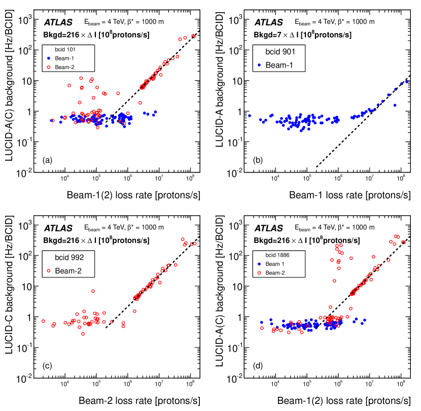
Figure 38: Correlation between beam loss rate and the background rates measured by LUCID in the two paired BCIDs 101 (a) and 1886 (d) and two unpaired BCIDs 901 for beam-1 (b) and 992 for beam-2 (c). The data-points falling on the horizontal at small loss rates represent the normal beam-gas and noise level. The points on the diagonal are associated to large losses due to cleaning in IR7. The dashed line is not a fit to the data, but just gives an indication of the slope. Especially in BCID 1886 some large background is seen also for small beam intensity loss. This is due to cleaning in IR3.

Figure 38 shows the correlation between the bunch intensity loss rate and the BIB rate observed by LUCID. The dashed lines in the plots are only to guide the eye, but they indicate that for a given beam the correlation is the same for each BCID, while it differs for the two beams. In particular, a comparison of figure 38(b) with the other three plots of figure 38 confirms that the ratio between background and beam loss is about a factor of 30 smaller for beam-1 than for beam-2. A value, perfectly consistent with that derived above from height-differences of individual peaks in figure 36.

The large group of outlier points with high background $(\sim\!10^{2}$ Hz/BCID) but moderate loss rate $(\sim\!10^{6})$ protons/s, seen in figure 38(d) for BCID 1886 in beam-2 direction, corresponds to the high background seen in figure 36(d) between 20:15 and 20:25 UTC. At this time IR7 collimators were still open, so it seems evident that this background is due to scraping away off-momentum tails when the IR3 collimators close.

The background seen by the BCM was found to exhibit very similar behaviour to that observed in figure 38.

In conclusion, it is observed that at least in the 1000 m optics ATLAS is much more sensitive to losses in IR3 than in IR7. In fact the sensitivity is larger to beam-2 losses in IR7, a fraction of which leak to IR3 and from there to ATLAS, than to direct debris from beam-1 losses in IR7. This suggests that protons leaking out from IR7 are not intercepted to a significant degree by ATLAS (beam-1) or CMS (beam-2), but predominantly by IR3.

Finally, it should be remarked that despite the very different optics, the results in section 9 suggest that this larger sensitivity to IR3 losses could be present also in normal high-luminosity optics; as discussed in section 9 ghost-BIB is observed only in beam-2 and attributed to losses of ghost charge in IR3. Even during abort-gap cleaning, which should increase losses in IR7, the ATLAS backgrounds in beam-2 increased more. These indications together with the results obtained in this high-$\beta^{*}$ fill suggest that similar comparisons between cleaning losses and ATLAS backgrounds could be done in LHC Run-2 by recording background data during dedicated loss-map studies of the LHC.

10.3 Backgrounds during 25 ns operation

At the end of the 2012 $pp$ running the LHC operated for a few fills with a 25 ns bunch separation. The bunch pattern included 12 isolated bunches per beam, which were isolated by 88 BCIDs, i.e. much more than during 50 ns operation.

Figure 39 compares the L1_BCM_AC_CA rates in the unpaired isolated bunches for the 25 ns and 50 ns operation. The observed beam-gas rates for beam-1 are at a similar level in both cases. Unlike in the 50 ns operation, where the beam-1 rate was about 25% higher than that of beam-2, the 25 ns operation exhibits an opposite trend with the background rate from beam-2 being approximately 5% higher than that from beam-1.

Figure 39: Beam-gas rate per BCID in the events triggered by L1_AC_CA_UNPAIRED_ISO in the data with 50 ns (downward triangles) and 25 ns (upward triangles) bunch spacing. The BCID values corresponding to the unpaired bunches in the 50 ns (25 ns) data are indicated by the bottom (top) $x$-axis. For the 50 ns data only LHC fills with 1368 colliding bunches taken before the September technical stop are considered. Only the first well isolated unpaired bunches are shown for the bunch pattern used in the 25 ns fill.

11 Conclusions

A detailed analysis of beam-induced (BIB) and cosmic-ray backgrounds (CRB) in the ATLAS detector during the 2012 operation has been presented. The principal methods to monitor backgrounds in ATLAS rely on the existence of unpaired bunches in the fill pattern. The BIB rates associated with these are observed by the Beam Conditions Monitor (BCM) and fake jets with $p_{\rm T}>10$  in the calorimeters.

The observation, made already in 2011 background data that beam backgrounds seen by the BCM are strongly correlated with the residual pressure 22 m from the interaction point, is re-established and further elaborated. In particular, it is shown that a scaling of the BCM background with a linear combination of the pressures around the inner triplet results in a very constant rate throughout 2012. Any deviations from this constant level are sensitive indications of abnormal beam-losses.

The background data collected in 2012 benefited from an optimised bunch pattern with dedicated unpaired bunches, well separated from the colliding ones. Largely due to these cleaner conditions, the analysis of 2012 background data revealed features, related to ghost charge, which were not seen in the 2011 analysis. The most noteworthy observation is the high sensitivity of ATLAS to off-momentum ghost charge being lost in IR3. The debris from these cleaning losses is seen both by the BCM and as fake jets in the calorimeters. An analysis of these rates revealed a significant jump of BIB from beam-2 ghost charge in early August, coincident with the LHC changing chromaticities. BIB, due to ghost charge losses, could be observed in the $3\,\mu$s long abort gap and for beam-2 was found to exhibit an unexpected hump-structure following the chromaticity changes, but not before. During periods of dedicated abort gap cleaning by the LHC these losses increased. Immediately after the cleaning a reduction of background was observed, but only for the order of one minute. This suggests that the abort gap is filled by de-bunched beam with a time constant of the order of one minute.

BIB from ghost charge can also be observed in form of fake jets. This analysis benefits from the excellent time resolution of the ATLAS calorimeters, which allows use of the jet time to determine the direction of the BIB muon producing the fake jet.

Further analyses of the fake jet data show that after an initial decrease in early 2012 the rates remained constant throughout most of the year. Fake-jet data were also collected during dedicated CRB data-taking and the energy and multiplicity distributions of the reconstructed jets compare well with Monte Carlo results. After proper normalisation, the rates of fake jet rates due to BIB and CRB could be compared, showing that beyond $p_{\rm T}\sim 1\,$ the rates are similar, while at $p_{\rm T}\sim 200$ , the CRB-muons produce only 10% of the total fake jet rate.

Two LHC fills of particular interest were subject of more detailed investigation. One fill, with an abnormally high background in beam-1, revealed that an earlier quench of the inner triplet had caused adsorption of residual gas on the beam-screen. At the start of the next fill the collision debris hitting the beam screen caused desorption of this gas, which resulted in the observed background excess. The evolution of the background excess as a function of time provided information about the cleaning of the beam screen by the collision debris.

Another fill of interest is the one with high $\beta^{*}$ for total cross-section measurements by the ALFA and TOTEM detectors, characterised by a sparse bunch pattern and very low luminosity. Since ALFA and TOTEM approached with their detectors very close to the beam, the halo was periodically cleaned down to two nominal $\sigma$. During these cleaning periods significant fractions of the beam intensity were lost. At the same time background spikes were observed in ATLAS, establishing a correlation between cleaning losses and BIB in ATLAS, although only for this very special optics configuration.

The experience gained and observations made during this analysis allows for further improvements and better targeting of background monitoring methods and analysis tools for LHC Run-2. In particular monitoring of BIB from ghost charge was shown to provide useful insights. The results presented in this paper indicate that with the new analysis methods ATLAS can resolve low enough levels of BIB to facilitate participation in dedicated loss-map measurements of the accelerator in Run-2. Such measurements promise to grant further insights into sources of background and should allow better predictions of background levels for different collimator configurations.

On the physics side, an improved understanding of the properties of BIB and CRB provides the basis for further optimisation of background rejection techniques. With the 25ns bunch spacing and higher collision energies in LHC Run-2, such improved background rejection will be crucial in order to enhance sensitivity to beyond the Standard Model phenomena in various channels, such as unconventional signatures of non-prompt decays, as well as measurements involving high $p_{\rm T}$ jets.

Appendix A BCM trigger configurations in 2012

Until TS3, in mid-September, the BCM trigger was provided by the same read-out driver (ROD) as in 2011, called BCM PRO with the L1_BCM_Wide trigger window in bins 28–48. During TS3 the trigger was moved to use a new BCM DEV ROD with the L1_BCM_Wide window re-aligned to bins 36–50, i.e. the same as the in-time window of L1_BCM_AC_CA. Table 4 summarises the windows of the BCM level-1 and luminosity triggers.

Trigger	Type	Early window	In-time Window	comment
L1_BCM_AC_CA	Early & in-time	$-6.25\,\pm\,2.73$	$+6.25\,\pm\,2.73$	All 2012
L1_BCM_Wide	A&C coincidence	—	$+4.29\,\pm\,3.90$	Before TS3
L1_BCM_Wide	A&C coincidence	—	$+6.25\,\pm\,2.73$	After TS3
BCM_TORx	Single side A or C	—	$+6.25\,\pm\,6.25$	All 2012

Table 4: Summary of triggers used and their time windows (ns) with respect to the nominal collision time. The BCM_TORx is not a L1 trigger item, but the count rate provided for luminosity determination, which is used for some analyses of this paper.

An additional feature was that the collision-time in BCM DEV was shifted by roughly 6 bins with respect to BCM PRO. While triggers after TS3 were given by BCM DEV, the data used for the analysis of this paper was extracted from BCM PRO throughout 2012. The consequence is that in the data after TS3 the trigger windows appear shifted to bins 42–56 and 10–24.

The time distributions of the events before and after TS3 are illustrated in figure 40. Prior to TS3 a sharp lower edge in bin 28 is seen, corresponding to the start of the trigger window. The upper edge is after bin 48 and appears to cut the tail of the signal. After TS3 the lower edge is well aligned with the rising signal and thus not visible in the plot. The upper edge is seen after bin 56, which is far in the signal tail. This suggests that the signal is better contained in the trigger window after TS3. The impact on the efficiency cannot be exactly quantified, but is at most 10% (based on the size of the tail apparently cut off in the left plot). Since the effect cannot be quantified accurately, no correction has been explicitly applied, but an implicit accounting for it is described below.

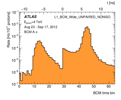
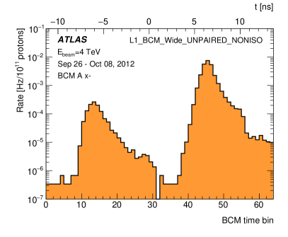
Figure 40: Response of the BCM $x-$ station on side A in the events triggered by L1_BCM_Wide_UNPAIRED_NONISO before (a) and after (b) the September technical stop.

A major difference between the two RODs is that the trigger in the old BCM PRO was treating the horizontal and vertical BCM modules independently - like two independent detectors, while the trigger in BCM DEV combined all modules together, which has a significant effect on the trigger acceptance.

Assuming that back-to-back correlations between the secondaries produced in minimum-bias $pp$ collision events are negligible, the BCM-Wide rate after the trigger change should increase by exactly a factor of two: if the (small) probability to produce a hit on one side in horizontal modules is denoted by $p$, then the probability for a coincidence is approximately $p^{2}$. Since the vertical modules have independently the same probability, the total is $2p^{2}$. After combining the modules in the BCM DEV, the probability for a hit on one side is $2p$ and the probability for coincidence is $4p^{2}$.

In order to verify that back-to-back correlations are negligible, and also to assess the possible efficiency impact of the trigger window re-alignment, the ratio between L1_BCM_Wide and L1_J10 rates before and after TS3 were compared. The result is shown in figure 41. Since no other changes to the system were made and beam conditions were comparable, the difference in this ratio allows to quantify the shift. Averaging the ratios before and after TS3, respectively, they are found to differ by a factor of $1.985\pm 0.021$. This confirms that a factor of two has to be applied to L1_BCM_Wide rates before TS3, in order to compensate for the effect of the trigger change.

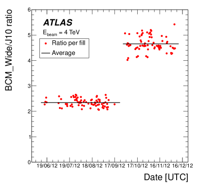
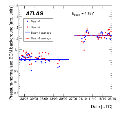
Figure 41: Ratio between BCM_Wide and J10 trigger rates before and after TS3 (a) and trend of BCM_AC_CA rates after scaling with the 22 m pressure (b).

It is more complicated to estimate the effect of the change on the BIB trigger L1_BCM_AC_CA, since it is designed to trigger on a correlation between early an in-time hits and there is no information how often such hits are produced by the same particle traversing upstream and downstream modules in the same azimuth. Any cross-talk between horizontal and vertical modules, e.g. by two different secondaries from the same event, would lead to an increase of the trigger rate in BCM DEV. The upper limit of the increase is a factor of 2, corresponding to fully uncorrelated hits in the modules. Unlike for the collision-dominated L1_BCM_Wide, there is no other rate to which the BCM background trigger could be compared. The raw L1_BCM_AC_CA data, even after bunch intensity normalisation, are found to have a scatter much larger than the effect of the trigger change. The method employed to reduce this scatter by taking into account the vacuum conditions is described in section 7.1. The normalization with the residual pressure produces a reasonably flat distribution before and after TS3, and allows deriving the change in L1_BCM_AC_CA rate to be a factor of $1.22\pm 0.01$ for beam-1 and $1.19\pm 0.01$ for beam-2. This is illustrated in figure 41. For simplicity a unique factor of 1.2 was applied to L1_BCM_AC_CA rates prior to TS3 for both beams.

In section 7.2 rates extracted from the luminosity data are compared to L1_BCM_Wide trigger rates. When doing this, the different window widths shown in table 4 have to be taken into account. Figure 40 indicates that the signal from collisions or in-time BIB (figure 5) is almost fully contained in the L1_BCM_Wide window – and of course in the wider BCM-TORx. The count rates for hits distributed randomly in time, e.g. afterglow_pp and noise, depend on the width of the windows and if these rates are to be compared an appropriate correction has to be applied. The BCM-TORx rates correspond to an acceptance window of 12.5 ns width, while the BCM_Wide window is only 5.1 ns wide, which implies that a correction factor of 0.41 has to be applied to pedestal hits distributed uniformly in time. Since no correction is needed for in-time BIB, the correction factor for random BIB+pedestal coincidences amounts to this 0.41. Pedestal+pedestal coincidences have to be corrected by $0.41^{2}=0.17$ when comparing rates derived from BCM-TORx to L1_BCM_Wide rates.

References

- [1] ATLAS Collaboration “Characterisation and mitigation of beam-induced backgrounds observed in the ATLAS detector during the 2011 proton-proton run” In JINST 8, 2013, pp. P07004 DOI: 10.1088/1748-0221/8/07/P07004
- [2] Lyndon R Evans and Philip Bryant “LHC Machine” This report is an abridged version of the LHC Design Report (CERN-2004-003) In J. Instrum. 3, 2008, pp. S08001. 164 p URL: https://cds.cern.ch/record/1129806
- [3] ATLAS Collaboration “The ATLAS Experiment at the CERN Large Hadron Collider” In JINST 3, 2008, pp. S08003 DOI: 10.1088/1748-0221/3/08/S08003
- [4] Oliver Sim Brüning et al. “LHC Design Report” Geneva: CERN, 2004 URL: https://cds.cern.ch/record/782076
- [5] R. Bruce “Simulations and measurements of beam loss patterns at the CERN Large Hadron Collider” In Phys. Rev. ST Accel. Beams 17, 2014, pp. 081004 DOI: 10.1103/PhysRevSTAB.17.081004
- [6] B Angerth et al. “The cold vacuum system of the Large Hadron Collider”, 1994, pp. 4 p URL: https://cds.cern.ch/record/268268
- [7] Cristoforo Benvenuti, P Chiggiato, F Cicora and V Ruzinov “Decreasing surface outgassing by thin film getter coatings” In Vacuum 50.1-2, 1998, pp. 57–63 URL: https://cds.cern.ch/record/364588
- [8] A. Jeff et al. “Longitudinal density monitor for the LHC” In Phys. Rev. ST Accel. Beams 15, 2012, pp. 032803 DOI: 10.1103/PhysRevSTAB.15.032803
- [9] Helmut Wiedemann “Particle Accelerator Physics”, Graduate Texts in Physics Berlin, Germany: Springer, 2015 DOI: 10.1007/978-3-319-18317-6
- [10] V. Cindro “The ATLAS beam conditions monitor” In JINST 3, 2008, pp. P02004 DOI: 10.1088/1748-0221/3/02/P02004
- [11] R. Bruce “Sources of machine-induced background in the ATLAS and CMS detectors at the CERN Large Hadron Collider” In Nucl. Instrum. Meth. A729, 2013, pp. 825–840 DOI: 10.1016/j.nima.2013.08.058
- [12] A I Drozhdin, N V Mokhov and S I Striganov “Beam Losses and Background Loads on Collider Detectors Due to Beam-Gas Interactions in the LHC”, 2010 URL: https://cds.cern.ch/record/1370157
- [13] ATLAS Collaboration “Search for new phenomena in final states with an energetic jet and large missing transverse momentum in pp collisions at 8 TeV with the ATLAS detector” [Erratum: Eur. Phys. J.C75,no.9,408(2015)] In Eur. Phys. J. C75.7, 2015, pp. 299 DOI: 10.1140/epjc/s10052-015-3517-3, 10.1140/epjc/s10052-015-3639-7
- [14] ATLAS Collaboration “Search for long-lived stopped R-hadrons decaying out-of-time with pp collisions using the ATLAS detector” In Phys. Rev. D88.11, 2013, pp. 112003 DOI: 10.1103/PhysRevD.88.112003
- [15] ATLAS Collaboration “Improved luminosity determination in pp collisions at sqrt(s) = 7 TeV using the ATLAS detector at the LHC” In Eur. Phys. J. C73.8, 2013, pp. 2518 DOI: 10.1140/epjc/s10052-013-2518-3
- [16] F Blas et al. “Conversion of the PS complex as LHC proton pre-injector”, 1997, pp. 3 p URL: https://cds.cern.ch/record/328735
- [17] Stéphane David Fartoukh, Jean Bernard Jeanneret and Elena Shaposhnikova “LHC Abort Gap Filling by Proton Beam” revised version submitted on 2004-09-23 11:55:00, 2004, pp. 4 p URL: https://cds.cern.ch/record/790609
- [18] Elena Shaposhnikova, pivate communication
- [19] ATLAS Collaboration “Jet energy measurement and its systematic uncertainty in proton-proton collisions at TeV with the ATLAS detector” In Eur. Phys. J. C75, 2015, pp. 17 DOI: 10.1140/epjc/s10052-014-3190-y
- [20] ATLAS Collaboration “Monitoring and data quality assessment of the ATLAS liquid argon calorimeter” In JINST 9, 2014, pp. P07024 DOI: 10.1088/1748-0221/9/07/P07024
- [21] Matteo Cacciari, Gavin P. Salam and Gregory Soyez “The Anti-k(t) jet clustering algorithm” In JHEP 04, 2008, pp. 063 DOI: 10.1088/1126-6708/2008/04/063
- [22] E Metral “Review of the instabilities observed during the 2012 run and actions taken”, unpublished, 2012 URL: http://indico.cern.ch/event/211614/session/5/contribution/17/attachments/332063/463333/Evian_Dec2012-EM_Final.pdf
- [23] ATLAS Collaboration “Luminosity Determination in Collisions at TeV Using the ATLAS Detector at the LHC” In Eur. Phys. J. C71, 2011, pp. 1630 DOI: 10.1140/epjc/s10052-011-1630-5
- [24] ATLAS Collaboration “Performance of Missing Transverse Momentum Reconstruction in Proton-Proton Collisions at 7 TeV with ATLAS” In Eur. Phys. J. C72, 2012, pp. 1844 DOI: 10.1140/epjc/s10052-011-1844-6
- [25] T. Gleisberg et al. “Event generation with SHERPA 1.1” In JHEP 02, 2009, pp. 007 DOI: 10.1088/1126-6708/2009/02/007
- [26] Hung-Liang Lai et al. “New parton distributions for collider physics” In Phys. Rev. D82, 2010, pp. 074024 DOI: 10.1103/PhysRevD.82.074024
- [27] Stefano Catani and Massimiliano Grazzini “An NNLO subtraction formalism in hadron collisions and its application to Higgs boson production at the LHC” In Phys. Rev. Lett. 98, 2007, pp. 222002 DOI: 10.1103/PhysRevLett.98.222002
- [28] Stefano Catani et al. “Vector boson production at hadron colliders: a fully exclusive QCD calculation at NNLO” In Phys. Rev. Lett. 103, 2009, pp. 082001 DOI: 10.1103/PhysRevLett.103.082001
- [29] A. D. Martin, W. J. Stirling, R. S. Thorne and G. Watt “Parton distributions for the LHC” In Eur. Phys. J. C63, 2009, pp. 189–285 DOI: 10.1140/epjc/s10052-009-1072-5
- [30] S. Agostinelli “GEANT4: A Simulation toolkit” In Nucl. Instrum. Meth. A506, 2003, pp. 250–303 DOI: 10.1016/S0168-9002(03)01368-8
- [31] T. K. Gaisser “Cosmic rays and particle physics” In Cambridge, UK: Univ. Pr. (1990) 279 p, 1990 URL: http://www.cambridge.org/uk/catalogue/catalogue.asp?isbn=0521326672
- [32] S. R. Kelner, R. P. Kokoulin and A. A. Petrukhin “Bremsstrahlung from muons scattered by atomic electrons” [Yad. Fiz.60,657(1997)] In Phys. Atom. Nucl. 60, 1997, pp. 576–583
- [33] A. Dar “Atmospheric Neutrinos, Astrophysical Neutrinos and Proton Decay Experiments” [,101(1983)] In Fourth Workshop on Grand Unification Philadelphia, Pennsylvania., April 21-23, 1983 51, 1983, pp. 227 DOI: 10.1103/PhysRevLett.51.227
- [34] L3 Collaboration “Measurement of the atmospheric muon spectrum from 20-GeV to 3000-GeV” In Phys. Lett. B598, 2004, pp. 15–32 DOI: 10.1016/j.physletb.2004.08.003
- [35] V. Avati et al. “Cosmic multi-muon events observed in the underground CERN-LEP tunnel with the ALEPH experiment” In Astropart. Phys. 19, 2003, pp. 513–523 DOI: 10.1016/S0927-6505(02)00247-5
- [36] DELPHI Collaboration “Study of multi-muon bundles in cosmic ray showers detected with the DELPHI detector at LEP” In Astropart. Phys. 28, 2007, pp. 273–286 DOI: 10.1016/j.astropartphys.2007.06.001
- [37] B Salvachua et al. “Estimate of Warm Magnets Lifetime in the Betatron and Momentum Cleaning Insertions of the LHC”, 2013, pp. 3 p URL: https://cds.cern.ch/record/1574597
- [38] E Metral et al. “Summary of the 2-day internal review of LHC performance limitations (linked to transverse collective effects) during run I (CERN, 25-26/09/2013)”, 2014 URL: https://cds.cern.ch/record/1645854
- [39] Malika Meddahi “LHC Abort Gap Monitoring and Cleaning” In Proceedings, 1st International Particle Accelerator Conference (IPAC’10) C100523, 2010, pp. MOPEC009
- [40] ATLAS Collaboration “Measurement of the total cross section from elastic scattering in pp collisions at TeV with the ATLAS detector” In Nucl. Phys. B889, 2014, pp. 486–548 DOI: 10.1016/j.nuclphysb.2014.10.019
- [41] TOTEM Collaboration “The TOTEM experiment at the CERN Large Hadron Collider” In JINST 3, 2008, pp. S08007 DOI: 10.1088/1748-0221/3/08/S08007
- [42] TOTEM Collaboration “Performance of the TOTEM Detectors at the LHC” In Int. J. Mod. Phys. A28, 2013, pp. 1330046 DOI: 10.1142/S0217751X13300469
- [43] Roderik Bruce “SixTrack Simulations of Beam Cleaning During High-beta Operation in the LHC” In Proceedings, 6th International Particle Accelerator Conference (IPAC 2015), 2015, pp. TUPTY027 URL: http://accelconf.web.cern.ch/AccelConf/IPAC2015/papers/tupty027.pdf
The ATLAS Collaboration
G. Aad, B. Abbott, J. Abdallah, O. Abdinov, B. Abeloos, R. Aben, M. Abolins, O.S. AbouZeid, N.L. Abraham, H. Abramowicz, H. Abreu, R. Abreu, Y. Abulaiti, B.S. Acharya,a, L. Adamczyk, D.L. Adams, J. Adelman, S. Adomeit, T. Adye, A.A. Affolder, T. Agatonovic-Jovin, J. Agricola, J.A. Aguilar-Saavedra, S.P. Ahlen, F. Ahmadov,b, G. Aielli, H. Akerstedt, T.P.A. Åkesson, A.V. Akimov, G.L. Alberghi, J. Albert, S. Albrand, M.J. Alconada Verzini, M. Aleksa, I.N. Aleksandrov, C. Alexa, G. Alexander, T. Alexopoulos, M. Alhroob, M. Aliev, G. Alimonti, J. Alison, S.P. Alkire, B.M.M. Allbrooke, B.W. Allen, P.P. Allport, A. Aloisio, A. Alonso, F. Alonso, C. Alpigiani, B. Alvarez Gonzalez, D. Álvarez Piqueras, M.G. Alviggi, B.T. Amadio, K. Amako, Y. Amaral Coutinho, C. Amelung, D. Amidei, S.P. Amor Dos Santos, A. Amorim, S. Amoroso, N. Amram, G. Amundsen, C. Anastopoulos, L.S. Ancu, N. Andari, T. Andeen, C.F. Anders, G. Anders, J.K. Anders, K.J. Anderson, A. Andreazza, V. Andrei, S. Angelidakis, I. Angelozzi, P. Anger, A. Angerami, F. Anghinolfi, A.V. Anisenkov,c, N. Anjos, A. Annovi, M. Antonelli, A. Antonov, J. Antos, F. Anulli, M. Aoki, L. Aperio Bella, G. Arabidze, Y. Arai, J.P. Araque, A.T.H. Arce, F.A. Arduh, G. Arduinid, J-F. Arguin, S. Argyropoulos, M. Arik, A.J. Armbruster, L.J. Armitage, O. Arnaez, H. Arnold, M. Arratia, O. Arslan, A. Artamonov, G. Artoni, S. Artz, S. Asai, N. Asbah, A. Ashkenazi, B. Åsman, L. Asquith, K. Assamagan, R. Astalos, M. Atkinson, N.B. Atlay, K. Augsten, G. Avolio, B. Axen, M.K. Ayoub, G. Azuelos,e, M.A. Baak, A.E. Baas, M.J. Baca, H. Bachacou, K. Bachas, M. Backes, M. Backhaus, P. Bagiacchi, P. Bagnaia, Y. Bai, J.T. Baines, O.K. Baker, E.M. Baldin,c, P. Balek, T. Balestri, F. Balli, W.K. Balunas, E. Banas, Sw. Banerjee,f, A.A.E. Bannoura, L. Barak, E.L. Barberio, D. Barberis, M. Barbero, T. Barillari, T. Barklow, N. Barlow, S.L. Barnes, B.M. Barnett, R.M. Barnett, Z. Barnovska, A. Baroncelli, G. Barone, A.J. Barr, L. Barranco Navarro, F. Barreiro, J. Barreiro Guimarães da Costa, R. Bartoldus, A.E. Barton, P. Bartos, A. Basalaev, A. Bassalat, A. Basye, R.L. Bates, S.J. Batista, J.R. Batley, M. Battaglia, M. Bauce, F. Bauer, H.S. Bawa,g, J.B. Beacham, M.D. Beattie, T. Beau, P.H. Beauchemin, P. Bechtle, H.P. Beck,h, K. Becker, M. Becker, M. Beckingham, C. Becot, A.J. Beddall, A. Beddall, V.A. Bednyakov, M. Bedognetti, C.P. Bee, L.J. Beemster, T.A. Beermann, M. Begel, J.K. Behr, C. Belanger-Champagne, A.S. Bell, G. Bella, L. Bellagamba, A. Bellerive, M. Bellomo, K. Belotskiy, O. Beltramello, N.L. Belyaev, O. Benary, D. Benchekroun, M. Bender, K. Bendtz, N. Benekos, Y. Benhammou, E. Benhar Noccioli, J. Benitez, J.A. Benitez Garcia, D.P. Benjamin, J.R. Bensinger, S. Bentvelsen, L. Beresford, M. Beretta, D. Berge, E. Bergeaas Kuutmann, N. Berger, F. Berghaus, J. Beringer, S. Berlendis, N.R. Bernard, C. Bernius, F.U. Bernlochner, T. Berry, P. Berta, C. Bertella, G. Bertoli, F. Bertolucci, I.A. Bertram, C. Bertsche, D. Bertsche, G.J. Besjes, O. Bessidskaia Bylund, M. Bessner, N. Besson, C. Betancourt, S. Bethke, A.J. Bevan, W. Bhimji, R.M. Bianchi, L. Bianchini, M. Bianco, O. Biebel, D. Biedermann, R. Bielski, N.V. Biesuz, M. Biglietti, J. Bilbao De Mendizabal, H. Bilokon, M. Bindi, S. Binet, A. Bingul, C. Bini, S. Biondi, D.M. Bjergaard, C.W. Black, J.E. Black, K.M. Black, D. Blackburn, R.E. Blair, J.-B. Blanchard, J.E. Blanco, T. Blazek, I. Bloch, C. Blocker, W. Blum,∗, U. Blumenschein, S. Blunier, G.J. Bobbink, V.S. Bobrovnikov,c, S.S. Bocchetta, A. Bocci, C. Bock, M. Boehler, D. Boerner, J.A. Bogaerts, D. Bogavac, A.G. Bogdanchikov, C. Bohm, V. Boisvert, T. Bold, V. Boldea, A.S. Boldyrev, M. Bomben, M. Bona, M. Boonekamp, A. Borisov, G. Borissov, J. Bortfeldt, D. Bortoletto, V. Bortolotto, K. Bos, D. Boscherini, M. Bosman, J.D. Bossio Sola, J. Boudreau, J. Bouffard, E.V. Bouhova-Thacker, D. Boumediene, C. Bourdarios, S.K. Boutle, A. Boveia, J. Boyd, I.R. Boyko, J. Bracinik, A. Brandt, G. Brandt, O. Brandt, U. Bratzler, B. Brau, J.E. Brau, H.M. Braun,∗, W.D. Breaden Madden, K. Brendlinger, A.J. Brennan, L. Brenner, R. Brenner, S. Bressler, T.M. Bristow, D. Britton, D. Britzger, F.M. Brochu, I. Brock, R. Brock, G. Brooijmans, T. Brooks, W.K. Brooks, J. Brosamer, E. Brost, J.H Broughton, R. Bruce, P.A. Bruckman de Renstrom, D. Bruncko, R. Bruneliere, A. Bruni, G. Bruni, BH Brunt, M. Bruschi, N. Bruscino, P. Bryant, L. Bryngemark, T. Buanes, Q. Buat, P. Buchholz, A.G. Buckley, I.A. Budagov, F. Buehrer, M.K. Bugge, O. Bulekov, D. Bullock, H. Burckhart, S. Burdin, C.D. Burgard, B. Burghgrave, K. Burka, S. Burke, I. Burmeister, E. Busato, D. Büscher, V. Büscher, P. Bussey, J.M. Butler, A.I. Butt, C.M. Buttar, J.M. Butterworth, P. Butti, W. Buttinger, A. Buzatu, A.R. Buzykaev,c, S. Cabrera Urbán, D. Caforio, V.M. Cairo, O. Cakir, N. Calace, P. Calafiura, A. Calandri, G. Calderini, P. Calfayan, L.P. Caloba, D. Calvet, S. Calvet, T.P. Calvet, R. Camacho Toro, S. Camarda, P. Camarri, D. Cameron, R. Caminal Armadans, C. Camincher, S. Campana, M. Campanelli, A. Campoverde, V. Canale, A. Canepa, M. Cano Bret, J. Cantero, R. Cantrill, T. Cao, M.D.M. Capeans Garrido, I. Caprini, M. Caprini, M. Capua, R. Caputo, R.M. Carbone, R. Cardarelli, F. Cardillo, T. Carli, G. Carlino, L. Carminati, S. Caron, E. Carquin, G.D. Carrillo-Montoya, J.R. Carter, J. Carvalho, D. Casadei, M.P. Casado,i, M. Casolino, D.W. Casper, E. Castaneda-Miranda, A. Castelli, V. Castillo Gimenez, N.F. Castro,j, A. Catinaccio, J.R. Catmore, A. Cattai, J. Caudron, V. Cavaliere, E. Cavallaro, D. Cavalli, M. Cavalli-Sforza, V. Cavasinni, F. Ceradini, L. Cerda Alberich, B.C. Cerio, A.S. Cerqueira, A. Cerri, L. Cerrito, F. Cerutti, M. Cerv, A. Cervelli, S.A. Cetin, A. Chafaq, D. Chakraborty, I. Chalupkova, S.K. Chan, Y.L. Chan, P. Chang, J.D. Chapman, D.G. Charlton, A. Chatterjee, C.C. Chau, C.A. Chavez Barajas, S. Che, S. Cheatham, A. Chegwidden, S. Chekanov, S.V. Chekulaev, G.A. Chelkov,k, M.A. Chelstowska, C. Chen, H. Chen, K. Chen, S. Chen, S. Chen, X. Chen, Y. Chen, H.C. Cheng, H.J Cheng, Y. Cheng, A. Cheplakov, E. Cheremushkina, R. Cherkaoui El Moursli, V. Chernyatin,∗, E. Cheu, L. Chevalier, V. Chiarella, G. Chiarelli, G. Chiodini, A.S. Chisholm, A. Chitan, M.V. Chizhov, K. Choi, A.R. Chomont, S. Chouridou, B.K.B. Chow, V. Christodoulou, D. Chromek-Burckhart, J. Chudoba, A.J. Chuinard, J.J. Chwastowski, L. Chytka, G. Ciapetti, A.K. Ciftci, D. Cinca, V. Cindro, I.A. Cioara, A. Ciocio, F. Cirotto, Z.H. Citron, M. Ciubancan, A. Clark, B.L. Clark, M.R. Clark, P.J. Clark, R.N. Clarke, C. Clement, Y. Coadou, M. Cobal, A. Coccaro, J. Cochran, L. Coffey, L. Colasurdo, B. Cole, S. Cole, A.P. Colijn, J. Collot, T. Colombo, G. Compostella, P. Conde Muiño, E. Coniavitis, S.H. Connell, I.A. Connelly, V. Consorti, S. Constantinescu, C. Conta, G. Conti, F. Conventi,l, M. Cooke, B.D. Cooper, A.M. Cooper-Sarkar, T. Cornelissen, M. Corradi, F. Corriveau,m, A. Corso-Radu, A. Cortes-Gonzalez, G. Cortiana, G. Costa, M.J. Costa, D. Costanzo, G. Cottin, G. Cowan, B.E. Cox, K. Cranmer, S.J. Crawley, G. Cree, S. Crépé-Renaudin, F. Crescioli, W.A. Cribbs, M. Crispin Ortuzar, M. Cristinziani, V. Croft, G. Crosetti, T. Cuhadar Donszelmann, J. Cummings, M. Curatolo, J. Cúth, C. Cuthbert, H. Czirr, P. Czodrowski, S. D’Auria, M. D’Onofrio, M.J. Da Cunha Sargedas De Sousa, C. Da Via, W. Dabrowski, T. Dai, O. Dale, F. Dallaire, C. Dallapiccola, M. Dam, J.R. Dandoy, N.P. Dang, A.C. Daniells, N.S. Dann, M. Danninger, M. Dano Hoffmann, V. Dao, G. Darbo, S. Darmora, J. Dassoulas, A. Dattagupta, W. Davey, C. David, T. Davidek, M. Davies, P. Davison, Y. Davygora, E. Dawe, I. Dawson, R.K. Daya-Ishmukhametova, K. De, R. de Asmundis, A. De Benedetti, S. De Castro, S. De Cecco, N. De Groot, P. de Jong, H. De la Torre, F. De Lorenzi, D. De Pedis, A. De Salvo, U. De Sanctis, A. De Santo, J.B. De Vivie De Regie, W.J. Dearnaley, R. Debbe, C. Debenedetti, D.V. Dedovich, I. Deigaard, J. Del Peso, T. Del Prete, D. Delgove, F. Deliot, C.M. Delitzsch, M. Deliyergiyev, A. Dell’Acqua, L. Dell’Asta, M. Dell’Orso, M. Della Pietra,l, D. della Volpe, M. Delmastro, P.A. Delsart, C. Deluca, D.A. DeMarco, S. Demers, M. Demichev, A. Demilly, S.P. Denisov, D. Denysiuk, D. Derendarz, J.E. Derkaoui, F. Derue, P. Dervan, K. Desch, C. Deterre, K. Dette, P.O. Deviveiros, A. Dewhurst, S. Dhaliwal, A. Di Ciaccio, L. Di Ciaccio, W.K. Di Clemente, C. Di Donato, A. Di Girolamo, B. Di Girolamo, B. Di Micco, R. Di Nardo, A. Di Simone, R. Di Sipio, D. Di Valentino, C. Diaconu, M. Diamond, F.A. Dias, M.A. Diaz, E.B. Diehl, J. Dietrich, S. Diglio, A. Dimitrievska, J. Dingfelder, P. Dita, S. Dita, F. Dittus, F. Djama, T. Djobava, J.I. Djuvsland, M.A.B. do Vale, D. Dobos, M. Dobre, C. Doglioni, T. Dohmae, J. Dolejsi, Z. Dolezal, B.A. Dolgoshein,∗, M. Donadelli, S. Donati, P. Dondero, J. Donini, J. Dopke, A. Doria, M.T. Dova, A.T. Doyle, E. Drechsler, M. Dris, Y. Du, J. Duarte-Campderros, E. Duchovni, G. Duckeck, O.A. Ducu, D. Duda, A. Dudarev, L. Duflot, L. Duguid, M. Dührssen, M. Dunford, H. Duran Yildiz, M. Düren, A. Durglishvili, D. Duschinger, B. Dutta, M. Dyndal, C. Eckardt, K.M. Ecker, R.C. Edgar, W. Edson, N.C. Edwards, T. Eifert, G. Eigen, K. Einsweiler, T. Ekelof, M. El Kacimi, V. Ellajosyula, M. Ellert, S. Elles, F. Ellinghaus, A.A. Elliot, N. Ellis, J. Elmsheuser, M. Elsing, D. Emeliyanov, Y. Enari, O.C. Endner, M. Endo, J.S. Ennis, J. Erdmann, A. Ereditato, G. Ernis, J. Ernst, M. Ernst, S. Errede, E. Ertel, M. Escalier, H. Esch, C. Escobar, B. Esposito, A.I. Etienvre, E. Etzion, H. Evans, A. Ezhilov, F. Fabbri, L. Fabbri, G. Facini, R.M. Fakhrutdinov, S. Falciano, R.J. Falla, J. Faltova, Y. Fang, M. Fanti, A. Farbin, A. Farilla, C. Farina, T. Farooque, S. Farrell, S.M. Farrington, P. Farthouat, F. Fassi, P. Fassnacht, D. Fassouliotis, M. Faucci Giannelli, A. Favareto, W.J. Fawcett, L. Fayard, O.L. Fedin,n, W. Fedorko, S. Feigl, L. Feligioni, C. Feng, E.J. Feng, H. Feng, A.B. Fenyuk, L. Feremenga, P. Fernandez Martinez, S. Fernandez Perez, J. Ferrando, A. Ferrari, P. Ferrari, R. Ferrari, D.E. Ferreira de Lima, A. Ferrer, D. Ferrere, C. Ferretti, A. Ferretto Parodi, F. Fiedler, A. Filipčič, M. Filipuzzi, F. Filthaut, M. Fincke-Keeler, K.D. Finelli, M.C.N. Fiolhais, L. Fiorini, A. Firan, A. Fischer, C. Fischer, J. Fischer, W.C. Fisher, N. Flaschel, I. Fleck, P. Fleischmann, G.T. Fletcher, G. Fletcher, R.R.M. Fletcher, T. Flick, A. Floderus, L.R. Flores Castillo, M.J. Flowerdew, G.T. Forcolin, A. Formica, A. Forti, A.G. Foster, D. Fournier, H. Fox, S. Fracchia, P. Francavilla, M. Franchini, D. Francis, L. Franconi, M. Franklin, M. Frate, M. Fraternali, D. Freeborn, S.M. Fressard-Batraneanu, F. Friedrich, D. Froidevaux, J.A. Frost, C. Fukunaga, E. Fullana Torregrosa, T. Fusayasu, J. Fuster, C. Gabaldon, O. Gabizon, A. Gabrielli, A. Gabrielli, G.P. Gach, S. Gadatsch, S. Gadomski, G. Gagliardi, L.G. Gagnon, P. Gagnon, C. Galea, B. Galhardo, E.J. Gallas, B.J. Gallop, P. Gallus, G. Galster, K.K. Gan, J. Gao, Y. Gao, Y.S. Gao,g, F.M. Garay Walls, C. García, J.E. García Navarro, M. Garcia-Sciveres, R.W. Gardner, N. Garelli, V. Garonne, A. Gascon Bravo, C. Gatti, A. Gaudiello, G. Gaudio, B. Gaur, L. Gauthier, I.L. Gavrilenko, C. Gay, G. Gaycken, E.N. Gazis, Z. Gecse, C.N.P. Gee, Ch. Geich-Gimbel, M.P. Geisler, C. Gemme, M.H. Genest, C. Geng,o, S. Gentile, S. George, D. Gerbaudo, A. Gershon, S. Ghasemi, H. Ghazlane, M. Ghneimat, B. Giacobbe, S. Giagu, P. Giannetti, B. Gibbard, S.M. Gibson, M. Gignac, M. Gilchriese, T.P.S. Gillam, D. Gillberg, G. Gilles, D.M. Gingrich,e, N. Giokaris, M.P. Giordani, F.M. Giorgi, F.M. Giorgi, P.F. Giraud, P. Giromini, D. Giugni, F. Giuli, C. Giuliani, M. Giulini, B.K. Gjelsten, S. Gkaitatzis, I. Gkialas, E.L. Gkougkousis, L.K. Gladilin, C. Glasman, J. Glatzer, P.C.F. Glaysher, A. Glazov, M. Goblirsch-Kolb, J. Godlewski, S. Goldfarb, T. Golling, D. Golubkov, A. Gomes, R. Gonçalo, J. Goncalves Pinto Firmino Da Costa, L. Gonella, A. Gongadze, S. González de la Hoz, G. Gonzalez Parra, S. Gonzalez-Sevilla, L. Goossens, P.A. Gorbounov, H.A. Gordon, I. Gorelov, B. Gorini, E. Gorini, A. Gorišek, E. Gornicki, A.T. Goshaw, C. Gössling, M.I. Gostkin, C.R. Goudet, D. Goujdami, A.G. Goussiou, N. Govender, E. Gozani, L. Graber, I. Grabowska-Bold, P.O.J. Gradin, P. Grafström, J. Gramling, E. Gramstad, S. Grancagnolo, V. Gratchev, H.M. Gray, E. Graziani, Z.D. Greenwood,p, C. Grefe, K. Gregersen, I.M. Gregor, P. Grenier, K. Grevtsov, J. Griffiths, A.A. Grillo, K. Grimm, S. Grinstein,q, Ph. Gris, J.-F. Grivaz, S. Groh, J.P. Grohs, E. Gross, J. Grosse-Knetter, G.C. Grossi, Z.J. Grout, L. Guan, W. Guan, J. Guenther, F. Guescini, D. Guest, O. Gueta, E. Guido, T. Guillemin, S. Guindon, U. Gul, C. Gumpert, J. Guo, Y. Guo,o, S. Gupta, G. Gustavino, P. Gutierrez, N.G. Gutierrez Ortiz, C. Gutschow, C. Guyot, C. Gwenlan, C.B. Gwilliam, A. Haas, C. Haber, H.K. Hadavand, N. Haddad, A. Hadef, P. Haefner, S. Hageböck, Z. Hajduk, H. Hakobyan,∗, M. Haleem, J. Haley, D. Hall, G. Halladjian, G.D. Hallewell, K. Hamacher, P. Hamal, K. Hamano, A. Hamilton, G.N. Hamity, P.G. Hamnett, L. Han, K. Hanagaki,r, K. Hanawa, M. Hance, B. Haney, P. Hanke, R. Hanna, J.B. Hansen, J.D. Hansen, M.C. Hansen, P.H. Hansen, K. Hara, A.S. Hard, T. Harenberg, F. Hariri, S. Harkusha, R.D. Harrington, P.F. Harrison, F. Hartjes, M. Hasegawa, Y. Hasegawa, A. Hasib, S. Hassani, S. Haug, R. Hauser, L. Hauswald, M. Havranek, C.M. Hawkes, R.J. Hawkings, A.D. Hawkins, D. Hayden, C.P. Hays, J.M. Hays, H.S. Hayward, S.J. Haywood, S.J. Head, T. Heck, V. Hedberg, L. Heelan, S. Heim, T. Heim, B. Heinemann, J.J. Heinrich, L. Heinrich, C. Heinz, J. Hejbal, L. Helary, S. Hellman, C. Helsens, J. Henderson, R.C.W. Henderson, Y. Heng, S. Henkelmann, A.M. Henriques Correia, S. Henrot-Versille, G.H. Herbert, Y. Hernández Jiménez, G. Herten, R. Hertenberger, L. Hervas, G.G. Hesketh, N.P. Hessey, J.W. Hetherly, R. Hickling, E. Higón-Rodriguez, E. Hill, J.C. Hill, K.H. Hiller, S.J. Hillier, I. Hinchliffe, E. Hines, R.R. Hinman, M. Hirose, D. Hirschbuehl, J. Hobbs, N. Hod, M.C. Hodgkinson, P. Hodgson, A. Hoecker, M.R. Hoeferkamp, F. Hoenig, M. Hohlfeld, D. Hohn, T.R. Holmes, M. Homann, T.M. Hong, B.H. Hooberman, W.H. Hopkins, Y. Horii, A.J. Horton, J-Y. Hostachy, S. Hou, A. Hoummada, J. Howard, J. Howarth, M. Hrabovsky, I. Hristova, J. Hrivnac, T. Hryn’ova, A. Hrynevich, C. Hsu, P.J. Hsu,s, S.-C. Hsu, D. Hu, Q. Hu, Y. Huang, Z. Hubacek, F. Hubaut, F. Huegging, T.B. Huffman, E.W. Hughes, G. Hughes, M. Huhtinen, T.A. Hülsing, N. Huseynov,b, J. Huston, J. Huth, G. Iacobucci, G. Iakovidis, I. Ibragimov, L. Iconomidou-Fayard, E. Ideal, Z. Idrissi, P. Iengo, O. Igonkina, T. Iizawa, Y. Ikegami, M. Ikeno, Y. Ilchenko,t, D. Iliadis, N. Ilic, T. Ince, G. Introzzi, P. Ioannou,∗, M. Iodice, K. Iordanidou, V. Ippolito, A. Irles Quiles, C. Isaksson, M. Ishino, M. Ishitsuka, R. Ishmukhametov, C. Issever, S. Istin, F. Ito, J.M. Iturbe Ponce, R. Iuppa, J. Ivarsson, W. Iwanski, H. Iwasaki, J.M. Izen, V. Izzo, S. Jabbar, B. Jackson, M. Jackson, P. Jackson, V. Jain, K.B. Jakobi, K. Jakobs, S. Jakobsen, T. Jakoubek, D.O. Jamin, D.K. Jana, E. Jansen, R. Jansky, J. Janssen, M. Janus, G. Jarlskog, N. Javadov,b, T. Javůrek, F. Jeanneau, L. Jeanty, J. Jejelava,u, G.-Y. Jeng, D. Jennens, P. Jenni,d, J. Jentzsch, C. Jeske, S. Jézéquel, H. Ji, J. Jia, H. Jiang, Y. Jiang, S. Jiggins, J. Jimenez Pena, S. Jin, A. Jinaru, O. Jinnouchi, P. Johansson, K.A. Johns, W.J. Johnson, K. Jon-And, G. Jones, R.W.L. Jones, S. Jones, T.J. Jones, J. Jongmanns, P.M. Jorge, J. Jovicevic, X. Ju, A. Juste Rozas,q, M.K. Köhler, A. Kaczmarska, M. Kado, H. Kagan, M. Kagan, S.J. Kahn, E. Kajomovitz, C.W. Kalderon, A. Kaluza, S. Kama, A. Kamenshchikov, N. Kanaya, S. Kaneti, V.A. Kantserov, J. Kanzaki, B. Kaplan, L.S. Kaplan, A. Kapliy, D. Kar, K. Karakostas, A. Karamaoun, N. Karastathis, M.J. Kareem, E. Karentzos, M. Karnevskiy, S.N. Karpov, Z.M. Karpova, K. Karthik, V. Kartvelishvili, A.N. Karyukhin, K. Kasahara, L. Kashif, R.D. Kass, A. Kastanas, Y. Kataoka, C. Kato, A. Katre, J. Katzy, K. Kawagoe, T. Kawamoto, G. Kawamura, S. Kazama, V.F. Kazanin,c, R. Keeler, R. Kehoe, J.S. Keller, J.J. Kempster, K Kentaro, H. Keoshkerian, O. Kepka, B.P. Kerševan, S. Kersten, R.A. Keyes, F. Khalil-zada, H. Khandanyan, A. Khanov, A.G. Kharlamov,c, T.J. Khoo, V. Khovanskiy, E. Khramov, J. Khubua,v, S. Kido, H.Y. Kim, S.H. Kim, Y.K. Kim, N. Kimura, O.M. Kind, B.T. King, M. King, S.B. King, J. Kirk, A.E. Kiryunin, T. Kishimoto, D. Kisielewska, F. Kiss, K. Kiuchi, O. Kivernyk, E. Kladiva, M.H. Klein, M. Klein, U. Klein, K. Kleinknecht, P. Klimek, A. Klimentov, R. Klingenberg, J.A. Klinger, T. Klioutchnikova, E.-E. Kluge, P. Kluit, S. Kluth, J. Knapik, E. Kneringer, E.B.F.G. Knoops, A. Knue, A. Kobayashi, D. Kobayashi, T. Kobayashi, M. Kobel, M. Kocian, P. Kodys, T. Koffas, E. Koffeman, L.A. Kogan, T. Koi, H. Kolanoski, M. Kolb, I. Koletsou, A.A. Komar,∗, Y. Komori, T. Kondo, N. Kondrashova, K. Köneke, A.C. König, T. Kono,w, R. Konoplich,x, N. Konstantinidis, R. Kopeliansky, S. Koperny, L. Köpke, A.K. Kopp, K. Korcyl, K. Kordas, A. Korn, A.A. Korol,c, I. Korolkov, E.V. Korolkova, O. Kortner, S. Kortner, T. Kosek, V.V. Kostyukhin, A. Kotwal, A. Kourkoumeli-Charalampidi, C. Kourkoumelis, V. Kouskoura, A. Koutsman, A.B. Kowalewska, R. Kowalewski, T.Z. Kowalski, W. Kozanecki, A.S. Kozhin, V.A. Kramarenko, G. Kramberger, D. Krasnopevtsev, M.W. Krasny, A. Krasznahorkay, J.K. Kraus, A. Kravchenko, M. Kretz, J. Kretzschmar, K. Kreutzfeldt, P. Krieger, K. Krizka, K. Kroeninger, H. Kroha, J. Kroll, J. Kroseberg, J. Krstic, U. Kruchonak, H. Krüger, N. Krumnack, A. Kruse, M.C. Kruse, M. Kruskal, T. Kubota, H. Kucuk, S. Kuday, J.T. Kuechler, S. Kuehn, A. Kugel, F. Kuger, A. Kuhl, T. Kuhl, V. Kukhtin, R. Kukla, Y. Kulchitsky, S. Kuleshov, M. Kuna, T. Kunigo, A. Kupco, H. Kurashige, Y.A. Kurochkin, V. Kus, E.S. Kuwertz, M. Kuze, J. Kvita, T. Kwan, D. Kyriazopoulos, A. La Rosa, J.L. La Rosa Navarro, L. La Rotonda, C. Lacasta, F. Lacava, J. Lacey, H. Lacker, D. Lacour, V.R. Lacuesta, E. Ladygin, R. Lafaye, B. Laforge, T. Lagouri, S. Lai, S. Lammers, W. Lampl, E. Lançon, U. Landgraf, M.P.J. Landon, V.S. Lang, J.C. Lange, A.J. Lankford, F. Lanni, K. Lantzsch, A. Lanza, S. Laplace, C. Lapoire, J.F. Laporte, T. Lari, F. Lasagni Manghi, M. Lassnig, P. Laurelli, W. Lavrijsen, A.T. Law, P. Laycock, T. Lazovich, M. Lazzaroni, O. Le Dortz, E. Le Guirriec, E. Le Menedeu, E.P. Le Quilleuc, M. LeBlanc, T. LeCompte, F. Ledroit-Guillon, C.A. Lee, S.C. Lee, L. Lee, G. Lefebvre, M. Lefebvre, F. Legger, C. Leggett, A. Lehan, G. Lehmann Miotto, X. Lei, W.A. Leight, A. Leisos,y, A.G. Leister, M.A.L. Leite, R. Leitner, D. Lellouch, B. Lemmer, K.J.C. Leney, T. Lenz, B. Lenzi, R. Leone, S. Leone, C. Leonidopoulos, S. Leontsinis, G. Lerner, C. Leroy, A.A.J. Lesage, C.G. Lester, M. Levchenko, J. Levêque, D. Levin, L.J. Levinson, M. Levy, A.M. Leyko, M. Leyton, B. Li,o, H. Li, H.L. Li, L. Li, L. Li, Q. Li, S. Li, X. Li, Y. Li, Z. Liang, H. Liao, B. Liberti, A. Liblong, P. Lichard, K. Lie, J. Liebal, W. Liebig, C. Limbach, A. Limosani, S.C. Lin,z, T.H. Lin, B.E. Lindquist, E. Lipeles, A. Lipniacka, M. Lisovyi, T.M. Liss, D. Lissauer, A. Lister, A.M. Litke, B. Liu,aa, D. Liu, H. Liu, H. Liu, J. Liu, J.B. Liu, K. Liu, L. Liu, M. Liu, M. Liu, Y.L. Liu, Y. Liu, M. Livan, A. Lleres, J. Llorente Merino, S.L. Lloyd, F. Lo Sterzo, E. Lobodzinska, P. Loch, W.S. Lockman, F.K. Loebinger, A.E. Loevschall-Jensen, K.M. Loew, A. Loginov, T. Lohse, K. Lohwasser, M. Lokajicek, B.A. Long, J.D. Long, R.E. Long, L. Longo, K.A. Looper, L. Lopes, D. Lopez Mateos, B. Lopez Paredes, I. Lopez Paz, A. Lopez Solis, J. Lorenz, N. Lorenzo Martinez, M. Losada, P.J. Lösel, X. Lou, A. Lounis, J. Love, P.A. Love, H. Lu, N. Lu, H.J. Lubatti, C. Luci, A. Lucotte, C. Luedtke, F. Luehring, W. Lukas, L. Luminari, O. Lundberg, B. Lund-Jensen, D. Lynn, R. Lysak, E. Lytken, V. Lyubushkin, H. Ma, L.L. Ma, Y. Ma, G. Maccarrone, A. Macchiolo, C.M. Macdonald, B. Maček, J. Machado Miguens, D. Madaffari, R. Madar, H.J. Maddocks, W.F. Mader, A. Madsen, J. Maeda, S. Maeland, T. Maeno, A. Maevskiy, E. Magradze, J. Mahlstedt, C. Maiani, C. Maidantchik, A.A. Maier, T. Maier, A. Maio, S. Majewski, Y. Makida, N. Makovec, B. Malaescu, Pa. Malecki, V.P. Maleev, F. Malek, U. Mallik, D. Malon, C. Malone, S. Maltezos, S. Malyukov, J. Mamuzic, G. Mancini, B. Mandelli, L. Mandelli, I. Mandić, J. Maneira, L. Manhaes de Andrade Filho, J. Manjarres Ramos, A. Mann, B. Mansoulie, R. Mantifel, M. Mantoani, S. Manzoni, L. Mapelli, G. Marceca, L. March, G. Marchiori, M. Marcisovsky, M. Marjanovic, D.E. Marley, F. Marroquim, S.P. Marsden, Z. Marshall, L.F. Marti, S. Marti-Garcia, B. Martin, T.A. Martin, V.J. Martin, B. Martin dit Latour, M. Martinez,q, S. Martin-Haugh, V.S. Martoiu, A.C. Martyniuk, M. Marx, F. Marzano, A. Marzin, L. Masetti, T. Mashimo, R. Mashinistov, J. Masik, A.L. Maslennikov,c, I. Massa, L. Massa, P. Mastrandrea, A. Mastroberardino, T. Masubuchi, P. Mättig, J. Mattmann, J. Maurer, S.J. Maxfield, D.A. Maximov,c, R. Mazini, S.M. Mazza, N.C. Mc Fadden, G. Mc Goldrick, S.P. Mc Kee, A. McCarn, R.L. McCarthy, T.G. McCarthy, L.I. McClymont, K.W. McFarlane,∗, J.A. Mcfayden, G. Mchedlidze, S.J. McMahon, R.A. McPherson,m, M. Medinnis, S. Meehan, S. Mehlhase, A. Mehta, K. Meier, C. Meineck, B. Meirose, B.R. Mellado Garcia, F. Meloni, A. Mengarelli, S. Menke, E. Meoni, K.M. Mercurio, S. Mergelmeyer, P. Mermod, L. Merola, C. Meroni, F.S. Merritt, A. Messina, J. Metcalfe, A.S. Mete, C. Meyer, C. Meyer, J-P. Meyer, J. Meyer, H. Meyer Zu Theenhausen, R.P. Middleton, S. Miglioranzi, L. Mijović, G. Mikenberg, M. Mikestikova, M. Mikuž, M. Milesi, A. Milic, D.W. Miller, C. Mills, A. Milov, D.A. Milstead, A.A. Minaenko, Y. Minami, I.A. Minashvili, A.I. Mincer, B. Mindur, M. Mineev, Y. Ming, L.M. Mir, K.P. Mistry, T. Mitani, J. Mitrevski, V.A. Mitsou, A. Miucci, P.S. Miyagawa, J.U. Mjörnmark, T. Moa, K. Mochizuki, S. Mohapatra, W. Mohr, S. Molander, R. Moles-Valls, R. Monden, M.C. Mondragon, K. Mönig, J. Monk, E. Monnier, A. Montalbano, J. Montejo Berlingen, F. Monticelli, S. Monzani, R.W. Moore, N. Morange, D. Moreno, M. Moreno Llácer, P. Morettini, D. Mori, T. Mori, M. Morii, M. Morinaga, V. Morisbak, S. Moritz, A.K. Morley, G. Mornacchi, J.D. Morris, S.S. Mortensen, L. Morvaj, M. Mosidze, J. Moss, K. Motohashi, R. Mount, E. Mountricha, S.V. Mouraviev,∗, E.J.W. Moyse, S. Muanza, R.D. Mudd, F. Mueller, J. Mueller, R.S.P. Mueller, T. Mueller, D. Muenstermann, P. Mullen, G.A. Mullier, F.J. Munoz Sanchez, J.A. Murillo Quijada, W.J. Murray, H. Musheghyan, M. Muskinja, A.G. Myagkov,ab, M. Myska, B.P. Nachman, O. Nackenhorst, J. Nadal, K. Nagai, R. Nagai,w, K. Nagano, Y. Nagasaka, K. Nagata, M. Nagel, E. Nagy, A.M. Nairz, Y. Nakahama, K. Nakamura, T. Nakamura, I. Nakano, H. Namasivayam, R.F. Naranjo Garcia, R. Narayan, D.I. Narrias Villar, I. Naryshkin, T. Naumann, G. Navarro, R. Nayyar, H.A. Neal, P.Yu. Nechaeva, T.J. Neep, P.D. Nef, A. Negri, M. Negrini, S. Nektarijevic, C. Nellist, A. Nelson, S. Nemecek, P. Nemethy, A.A. Nepomuceno, M. Nessi,ac, M.S. Neubauer, M. Neumann, R.M. Neves, P. Nevski, P.R. Newman, D.H. Nguyen, R.B. Nickerson, R. Nicolaidou, B. Nicquevert, J. Nielsen, A. Nikiforov, V. Nikolaenko,ab, I. Nikolic-Audit, K. Nikolopoulos, J.K. Nilsen, P. Nilsson, Y. Ninomiya, A. Nisati, R. Nisius, T. Nobe, L. Nodulman, M. Nomachi, I. Nomidis, T. Nooney, S. Norberg, M. Nordberg, N. Norjoharuddeen, O. Novgorodova, S. Nowak, M. Nozaki, L. Nozka, K. Ntekas, E. Nurse, F. Nuti, F. O’grady, D.C. O’Neil, A.A. O’Rourke, V. O’Shea, F.G. Oakham,e, H. Oberlack, T. Obermann, J. Ocariz, A. Ochi, I. Ochoa, J.P. Ochoa-Ricoux, S. Oda, S. Odaka, H. Ogren, A. Oh, S.H. Oh, C.C. Ohm, H. Ohman, H. Oide, H. Okawa, Y. Okumura, T. Okuyama, A. Olariu, L.F. Oleiro Seabra, S.A. Olivares Pino, D. Oliveira Damazio, A. Olszewski, J. Olszowska, A. Onofre, K. Onogi, P.U.E. Onyisi,t, C.J. Oram, M.J. Oreglia, Y. Oren, D. Orestano, N. Orlando, R.S. Orr, B. Osculati, R. Ospanov, G. Otero y Garzon, H. Otono, M. Ouchrif, F. Ould-Saada, A. Ouraou, K.P. Oussoren, Q. Ouyang, A. Ovcharova, M. Owen, R.E. Owen, V.E. Ozcan, N. Ozturk, K. Pachal, A. Pacheco Pages, C. Padilla Aranda, M. Pagáčová, S. Pagan Griso, F. Paige, P. Pais, K. Pajchel, G. Palacino, S. Palestini, M. Palka, D. Pallin, M. Palmd, A. Palma, E.St. Panagiotopoulou, C.E. Pandini, J.G. Panduro Vazquez, P. Pani, S. Panitkin, D. Pantea, L. Paolozzi, Th.D. Papadopoulou, K. Papageorgiou, A. Paramonov, D. Paredes Hernandez, A.J. Parker, M.A. Parker, K.A. Parker, F. Parodi, J.A. Parsons, U. Parzefall, V.R. Pascuzzi, E. Pasqualucci, S. Passaggio, F. Pastore,∗, Fr. Pastore, G. Pásztor,ad, S. Pataraia, N.D. Patel, J.R. Pater, T. Pauly, J. Pearce, B. Pearson, L.E. Pedersen, M. Pedersen, S. Pedraza Lopez, R. Pedro, S.V. Peleganchuk,c, D. Pelikan, O. Penc, C. Peng, H. Peng, J. Penwell, B.S. Peralva, M.M. Perego, D.V. Perepelitsa, E. Perez Codina, L. Perini, H. Pernegger, S. Perrella, R. Peschke, V.D. Peshekhonov, K. Peters, R.F.Y. Peters, B.A. Petersen, T.C. Petersen, E. Petit, A. Petridis, C. Petridou, P. Petroff, E. Petrolo, M. Petrov, F. Petrucci, N.E. Pettersson, A. Peyaud, R. Pezoa, P.W. Phillips, G. Piacquadio, E. Pianori, A. Picazio, E. Piccaro, M. Piccinini, M.A. Pickering, R. Piegaia, J.E. Pilcher, A.D. Pilkington, A.W.J. Pin, J. Pina, M. Pinamonti,ae, J.L. Pinfold, A. Pingel, S. Pires, H. Pirumov, M. Pitt, L. Plazak, M.-A. Pleier, V. Pleskot, E. Plotnikova, P. Plucinski, D. Pluth, R. Poettgen, L. Poggioli, D. Pohl, G. Polesello, A. Poley, A. Policicchio, R. Polifka, A. Polini, C.S. Pollard, V. Polychronakos, K. Pommès, L. Pontecorvo, B.G. Pope, G.A. Popeneciu, D.S. Popovic, A. Poppleton, S. Pospisil, K. Potamianos, I.N. Potrap, C.J. Potter, C.T. Potter, G. Poulard, J. Poveda, V. Pozdnyakov, M.E. Pozo Astigarraga, P. Pralavorio, A. Pranko, S. Prell, D. Price, L.E. Price, M. Primavera, S. Prince, M. Proissl, K. Prokofiev, F. Prokoshin, S. Protopopescu, J. Proudfoot, M. Przybycien, D. Puddu, D. Puldon, M. Purohit,af, P. Puzo, J. Qian, G. Qin, Y. Qin, A. Quadt, W.B. Quayle, M. Queitsch-Maitland, D. Quilty, S. Raddum, V. Radeka, V. Radescu, S.K. Radhakrishnan, P. Radloff, P. Rados, F. Ragusa, G. Rahal, J.A. Raine, S. Rajagopalan, M. Rammensee, C. Rangel-Smith, M.G. Ratti, F. Rauscher, S. Rave, T. Ravenscroft, M. Raymond, A.L. Read, N.P. Readioff, D.M. Rebuzzi, A. Redelbach, G. Redlinger, R. Reece, K. Reeves, L. Rehnisch, J. Reichert, H. Reisin, C. Rembser, H. Ren, M. Rescigno, S. Resconi, O.L. Rezanova,c, P. Reznicek, R. Rezvani, R. Richter, S. Richter, E. Richter-Was, O. Ricken, M. Ridel, P. Rieck, C.J. Riegel, J. Rieger, O. Rifki, M. Rijssenbeek, A. Rimoldi, L. Rinaldi, B. Ristić, E. Ritsch, I. Riu, F. Rizatdinova, E. Rizvi, C. Rizzi, S.H. Robertson,m, A. Robichaud-Veronneau, D. Robinson, J.E.M. Robinson, A. Robson, C. Roda, Y. Rodina, A. Rodriguez Perez, D. Rodriguez Rodriguez, S. Roe, C.S. Rogan, O. Røhne, A. Romaniouk, M. Romano, S.M. Romano Saez, E. Romero Adam, N. Rompotis, M. Ronzani, L. Roos, E. Ros, S. Rosati, K. Rosbach, P. Rose, O. Rosenthal, V. Rossetti, E. Rossi, L.P. Rossi, J.H.N. Rosten, R. Rosten, M. Rotaru, I. Roth, J. Rothberg, D. Rousseau, C.R. Royon, A. Rozanov, Y. Rozen, X. Ruan, F. Rubbo, I. Rubinskiy, V.I. Rud, M.S. Rudolph, F. Rühr, A. Ruiz-Martinez, Z. Rurikova, N.A. Rusakovich, A. Ruschke, H.L. Russell, J.P. Rutherfoord, N. Ruthmann, Y.F. Ryabov, M. Rybar, G. Rybkin, S. Ryu, A. Ryzhov, A.F. Saavedra, G. Sabato, S. Sacerdoti, H.F-W. Sadrozinski, R. Sadykov, F. Safai Tehrani, P. Saha, M. Sahinsoy, M. Saimpert, T. Saito, H. Sakamoto, Y. Sakurai, G. Salamanna, A. Salamon, J.E. Salazar Loyola, D. Salek, P.H. Sales De Bruin, D. Salihagic, A. Salnikov, J. Salt, D. Salvatore, F. Salvatore, A. Salvucci, A. Salzburger, D. Sammel, D. Sampsonidis, A. Sanchez, J. Sánchez, V. Sanchez Martinez, H. Sandaker, R.L. Sandbach, H.G. Sander, M.P. Sanders, M. Sandhoff, C. Sandoval, R. Sandstroem, D.P.C. Sankey, M. Sannino, A. Sansoni, C. Santoni, R. Santonico, H. Santos, I. Santoyo Castillo, K. Sapp, A. Sapronov, J.G. Saraiva, B. Sarrazin, O. Sasaki, Y. Sasaki, K. Sato, G. Sauvage,∗, E. Sauvan, G. Savage, P. Savard,e, C. Sawyer, L. Sawyer,p, J. Saxon, C. Sbarra, A. Sbrizzi, T. Scanlon, D.A. Scannicchio, M. Scarcella, V. Scarfone, J. Schaarschmidt, P. Schacht, D. Schaefer, R. Schaefer, J. Schaeffer, S. Schaepe, S. Schaetzel, U. Schäfer, A.C. Schaffer, D. Schaile, R.D. Schamberger, V. Scharf, V.A. Schegelsky, D. Scheirich, M. Schernau, C. Schiavi, C. Schillo, M. Schioppa, S. Schlenker, K. Schmieden, C. Schmitt, S. Schmitt, S. Schmitz, B. Schneider, Y.J. Schnellbach, U. Schnoor, L. Schoeffel, A. Schoening, B.D. Schoenrock, E. Schopf, A.L.S. Schorlemmer, M. Schott, J. Schovancova, S. Schramm, M. Schreyer, N. Schuh, M.J. Schultens, H.-C. Schultz-Coulon, H. Schulz, M. Schumacher, B.A. Schumm, Ph. Schune, C. Schwanenberger, A. Schwartzman, T.A. Schwarz, Ph. Schwegler, H. Schweiger, Ph. Schwemling, R. Schwienhorst, J. Schwindling, T. Schwindt, G. Sciolla, F. Scuri, F. Scutti, J. Searcy, P. Seema, S.C. Seidel, A. Seiden, F. Seifert, J.M. Seixas, G. Sekhniaidze, K. Sekhon, S.J. Sekula, D.M. Seliverstov,∗, N. Semprini-Cesari, C. Serfon, L. Serin, L. Serkin, M. Sessa, R. Seuster, H. Severini, T. Sfiligoj, F. Sforza, A. Sfyrla, E. Shabalina, N.W. Shaikh, L.Y. Shan, R. Shang, J.T. Shank, M. Shapiro, P.B. Shatalov, K. Shaw, S.M. Shaw, A. Shcherbakova, C.Y. Shehu, P. Sherwood, L. Shi,ag, S. Shimizu, C.O. Shimmin, M. Shimojima, M. Shiyakova,ah, A. Shmeleva, D. Shoaleh Saadi, M.J. Shochet, S. Shojaii, S. Shrestha, E. Shulga, M.A. Shupe, P. Sicho, P.E. Sidebo, O. Sidiropoulou, D. Sidorov, A. Sidoti, F. Siegert, Dj. Sijacki, J. Silva, S.B. Silverstein, V. Simak, O. Simard, Lj. Simic, S. Simion, E. Simioni, B. Simmons, D. Simon, M. Simon, P. Sinervo, N.B. Sinev, M. Sioli, G. Siragusa, S.Yu. Sivoklokov, J. Sjölin, T.B. Sjursen, M.B. Skinner, H.P. Skottowe, P. Skubic, M. Slater, T. Slavicek, M. Slawinska, K. Sliwa, R. Slovak, V. Smakhtin, B.H. Smart, L. Smestad, S.Yu. Smirnov, Y. Smirnov, L.N. Smirnova,ai, O. Smirnova, M.N.K. Smith, R.W. Smith, M. Smizanska, K. Smolek, A.A. Snesarev, G. Snidero, S. Snyder, R. Sobie,m, F. Socher, A. Soffer, D.A. Soh,ag, G. Sokhrannyi, C.A. Solans Sanchez, M. Solar, E.Yu. Soldatov, U. Soldevila, A.A. Solodkov, A. Soloshenko, O.V. Solovyanov, V. Solovyev, P. Sommer, H. Son, H.Y. Song,aj, A. Sood, A. Sopczak, V. Sopko, V. Sorin, D. Sosa, C.L. Sotiropoulou, R. Soualah, A.M. Soukharev,c, D. South, B.C. Sowden, S. Spagnolo, M. Spalla, M. Spangenberg, F. Spanò, D. Sperlich, F. Spettel, R. Spighi, G. Spigo, L.A. Spiller, M. Spousta, R.D. St. Denis,∗, A. Stabile, J. Stahlman, R. Stamen, S. Stamm, E. Stanecka, R.W. Stanek, C. Stanescu, M. Stanescu-Bellu, M.M. Stanitzki, S. Stapnes, E.A. Starchenko, G.H. Stark, J. Stark, P. Staroba, P. Starovoitov, S. Stärz, R. Staszewski, P. Steinberg, B. Stelzer, H.J. Stelzer, O. Stelzer-Chilton, H. Stenzel, G.A. Stewart, J.A. Stillings, M.C. Stockton, M. Stoebe, G. Stoicea, P. Stolte, S. Stonjek, A.R. Stradling, A. Straessner, M.E. Stramaglia, J. Strandberg, S. Strandberg, A. Strandlie, M. Strauss, P. Strizenec, R. Ströhmer, D.M. Strom, R. Stroynowski, A. Strubig, S.A. Stucci, B. Stugu, N.A. Styles, D. Su, J. Su, R. Subramaniam, S. Suchek, Y. Sugaya, M. Suk, V.V. Sulin, S. Sultansoy, T. Sumida, S. Sun, X. Sun, J.E. Sundermann, K. Suruliz, G. Susinno, M.R. Sutton, S. Suzuki, M. Svatos, M. Swiatlowski, I. Sykora, T. Sykora, D. Ta, C. Taccini, K. Tackmann, J. Taenzer, A. Taffard, R. Tafirout, N. Taiblum, H. Takai, R. Takashima, H. Takeda, T. Takeshita, Y. Takubo, M. Talby, A.A. Talyshev,c, J.Y.C. Tam, K.G. Tan, J. Tanaka, R. Tanaka, S. Tanaka, B.B. Tannenwald, S. Tapia Araya, S. Tapprogge, S. Tarem, G.F. Tartarelli, P. Tas, M. Tasevsky, T. Tashiro, E. Tassi, A. Tavares Delgado, Y. Tayalati, A.C. Taylor, G.N. Taylor, P.T.E. Taylor, W. Taylor, F.A. Teischinger, P. Teixeira-Dias, K.K. Temming, D. Temple, H. Ten Kate, P.K. Teng, J.J. Teoh, F. Tepel, S. Terada, K. Terashi, J. Terron, S. Terzo, M. Testa, R.J. Teuscher,m, T. Theveneaux-Pelzer, J.P. Thomas, J. Thomas-Wilsker, E.N. Thompson, P.D. Thompson, R.J. Thompson, A.S. Thompson, L.A. Thomsen, E. Thomson, M. Thomson, M.J. Tibbetts, R.E. Ticse Torres, V.O. Tikhomirov,ak, Yu.A. Tikhonov,c, S. Timoshenko, P. Tipton, S. Tisserant, K. Todome, T. Todorov,∗, S. Todorova-Nova, J. Tojo, S. Tokár, K. Tokushuku, E. Tolley, L. Tomlinson, M. Tomoto, L. Tompkins,al, K. Toms, B. Tong, E. Torrence, H. Torres, E. Torró Pastor, J. Toth,am, F. Touchard, D.R. Tovey, T. Trefzger, A. Tricoli, I.M. Trigger, S. Trincaz-Duvoid, M.F. Tripiana, W. Trischuk, B. Trocmé, A. Trofymov, C. Troncon, M. Trottier-McDonald, M. Trovatelli, L. Truong, M. Trzebinski, A. Trzupek, J.C-L. Tseng, P.V. Tsiareshka, G. Tsipolitis, N. Tsirintanis, S. Tsiskaridze, V. Tsiskaridze, E.G. Tskhadadze, K.M. Tsui, I.I. Tsukerman, V. Tsulaia, S. Tsuno, D. Tsybychev, A. Tudorache, V. Tudorache, A.N. Tuna, S.A. Tupputi, S. Turchikhin,ai, D. Turecek, D. Turgeman, R. Turra, A.J. Turvey, P.M. Tuts, M. Tyndel, G. Ucchielli, I. Ueda, R. Ueno, M. Ughetto, F. Ukegawa, G. Unal, A. Undrus, G. Unel, F.C. Ungaro, Y. Unno, C. Unverdorben, J. Urban, P. Urquijo, P. Urrejola, G. Usai, A. Usanova, L. Vacavant, V. Vacek, B. Vachon, C. Valderanis, E. Valdes Santurio, N. Valencic, S. Valentinetti, A. Valero, L. Valery, S. Valkar, S. Vallecorsa, J.A. Valls Ferrer, W. Van Den Wollenberg, P.C. Van Der Deijl, R. van der Geer, H. van der Graaf, N. van Eldik, P. van Gemmeren, J. Van Nieuwkoop, I. van Vulpen, M.C. van Woerden, M. Vanadia, W. Vandelli, R. Vanguri, A. Vaniachine, P. Vankov, G. Vardanyan, R. Vari, E.W. Varnes, T. Varol, D. Varouchas, A. Vartapetian, K.E. Varvell, J.G. Vasquez, F. Vazeille, T. Vazquez Schroeder, J. Veatch, L.M. Veloce, F. Veloso, S. Veneziano, A. Ventura, M. Venturi, N. Venturi, A. Venturini, V. Vercesi, M. Verducci, W. Verkerke, J.C. Vermeulen, A. Vest,an, M.C. Vetterli,e, O. Viazlo, I. Vichou, T. Vickey, O.E. Vickey Boeriu, G.H.A. Viehhauser, S. Viel, L. Vigani, R. Vigne, M. Villa, M. Villaplana Perez, E. Vilucchi, M.G. Vincter, V.B. Vinogradov, C. Vittori, I. Vivarelli, S. Vlachos, M. Vlasak, M. Vogel, P. Vokac, G. Volpi, M. Volpi, H. von der Schmitt, E. von Toerne, V. Vorobel, K. Vorobev, M. Vos, R. Voss, J.H. Vossebeld, N. Vranjes, M. Vranjes Milosavljevic, V. Vrba, M. Vreeswijk, R. Vuillermet, I. Vukotic, Z. Vykydal, P. Wagner, W. Wagner, H. Wahlberg, S. Wahrmund, J. Wakabayashi, J. Walder, R. Walker, W. Walkowiak, V. Wallangen, C. Wang, C. Wang, F. Wang, H. Wang, H. Wang, J. Wang, J. Wang, K. Wang, R. Wang, S.M. Wang, T. Wang, T. Wang, X. Wang, C. Wanotayaroj, A. Warburton, C.P. Ward, D.R. Wardrope, A. Washbrook, P.M. Watkins, A.T. Watson, I.J. Watson, M.F. Watson, G. Watts, S. Watts, B.M. Waugh, S. Webb, M.S. Weber, S.W. Weber, J.S. Webster, A.R. Weidberg, B. Weinert, J. Weingarten, C. Weiser, H. Weits, P.S. Wells, T. Wenaus, T. Wengler, S. Wenig, N. Wermes, M. Werner, P. Werner, M. Wessels, J. Wetter, K. Whalen, N.L. Whallon, A.M. Wharton, A. White, M.J. White, R. White, S. White, D. Whiteson, F.J. Wickens, W. Wiedenmann, M. Wielers, P. Wienemann, C. Wiglesworth, L.A.M. Wiik-Fuchs, A. Wildauer, F. Wilk, H.G. Wilkens, H.H. Williams, S. Williams, C. Willis, S. Willocq, J.A. Wilson, I. Wingerter-Seez, F. Winklmeier, O.J. Winston, B.T. Winter, M. Wittgen, J. Wittkowski, S.J. Wollstadt, M.W. Wolter, H. Wolters, B.K. Wosiek, J. Wotschack, M.J. Woudstra, K.W. Wozniak, M. Wu, M. Wu, S.L. Wu, X. Wu, Y. Wu, T.R. Wyatt, B.M. Wynne, S. Xella, D. Xu, L. Xu, B. Yabsley, S. Yacoob, R. Yakabe, D. Yamaguchi, Y. Yamaguchi, A. Yamamoto, S. Yamamoto, T. Yamanaka, K. Yamauchi, Y. Yamazaki, Z. Yan, H. Yang, H. Yang, Y. Yang, Z. Yang, W-M. Yao, Y.C. Yap, Y. Yasu, E. Yatsenko, K.H. Yau Wong, J. Ye, S. Ye, I. Yeletskikh, A.L. Yen, E. Yildirim, K. Yorita, R. Yoshida, K. Yoshihara, C. Young, C.J.S. Young, S. Youssef, D.R. Yu, J. Yu, J.M. Yu, J. Yu, L. Yuan, S.P.Y. Yuen, I. Yusuff,ao, B. Zabinski, R. Zaidan, A.M. Zaitsev,ab, N. Zakharchuk, J. Zalieckas, A. Zaman, S. Zambito, L. Zanello, D. Zanzi, C. Zeitnitz, M. Zeman, A. Zemla, J.C. Zeng, Q. Zeng, K. Zengel, O. Zenin, T. Ženiš, D. Zerwas, D. Zhang, F. Zhang, G. Zhang,aj, H. Zhang, J. Zhang, L. Zhang, R. Zhang, R. Zhang,ap, X. Zhang, Z. Zhang, X. Zhao, Y. Zhao, Z. Zhao, A. Zhemchugov, J. Zhong, B. Zhou, C. Zhou, L. Zhou, L. Zhou, M. Zhou, N. Zhou, C.G. Zhu, H. Zhu, J. Zhu, Y. Zhu, X. Zhuang, K. Zhukov, A. Zibell, D. Zieminska, N.I. Zimine, C. Zimmermann, S. Zimmermann, Z. Zinonos, M. Zinser, M. Ziolkowski, L. Živković, G. Zobernig, A. Zoccoli, M. zur Nedden, G. Zurzolo, L. Zwalinski.
1 Department of Physics, University of Adelaide, Adelaide, Australia
2 Physics Department, SUNY Albany, Albany NY, United States of America
3 Department of Physics, University of Alberta, Edmonton AB, Canada
4 (a) Department of Physics, Ankara University, Ankara; (b) Istanbul Aydin University, Istanbul; (c) Division of Physics, TOBB University of Economics and Technology, Ankara, Turkey
5 LAPP, CNRS/IN2P3 and Université Savoie Mont Blanc, Annecy-le-Vieux, France
6 High Energy Physics Division, Argonne National Laboratory, Argonne IL, United States of America
7 Department of Physics, University of Arizona, Tucson AZ, United States of America
8 Department of Physics, The University of Texas at Arlington, Arlington TX, United States of America
9 Physics Department, University of Athens, Athens, Greece
10 Physics Department, National Technical University of Athens, Zografou, Greece
11 Department of Physics, The University of Texas at Austin, Austin TX, United States of America
12 Institute of Physics, Azerbaijan Academy of Sciences, Baku, Azerbaijan
13 Institut de Física d’Altes Energies (IFAE), The Barcelona Institute of Science and Technology, Barcelona, Spain, Spain
14 Institute of Physics, University of Belgrade, Belgrade, Serbia
15 Department for Physics and Technology, University of Bergen, Bergen, Norway
16 Physics Division, Lawrence Berkeley National Laboratory and University of California, Berkeley CA, United States of America
17 Department of Physics, Humboldt University, Berlin, Germany
18 Albert Einstein Center for Fundamental Physics and Laboratory for High Energy Physics, University of Bern, Bern, Switzerland
19 School of Physics and Astronomy, University of Birmingham, Birmingham, United Kingdom
20 (a) Department of Physics, Bogazici University, Istanbul; (b) Department of Physics Engineering, Gaziantep University, Gaziantep; (d) Istanbul Bilgi University, Faculty of Engineering and Natural Sciences, Istanbul,Turkey; (e) Bahcesehir University, Faculty of Engineering and Natural Sciences, Istanbul, Turkey, Turkey
21 Centro de Investigaciones, Universidad Antonio Narino, Bogota, Colombia
22 (a) INFN Sezione di Bologna; (b) Dipartimento di Fisica e Astronomia, Università di Bologna, Bologna, Italy
23 Physikalisches Institut, University of Bonn, Bonn, Germany
24 Department of Physics, Boston University, Boston MA, United States of America
25 Department of Physics, Brandeis University, Waltham MA, United States of America
26 (a) Universidade Federal do Rio De Janeiro COPPE/EE/IF, Rio de Janeiro; (b) Electrical Circuits Department, Federal University of Juiz de Fora (UFJF), Juiz de Fora; (c) Federal University of Sao Joao del Rei (UFSJ), Sao Joao del Rei; (d) Instituto de Fisica, Universidade de Sao Paulo, Sao Paulo, Brazil
27 Physics Department, Brookhaven National Laboratory, Upton NY, United States of America
28 (a) Transilvania University of Brasov, Brasov, Romania; (b) National Institute of Physics and Nuclear Engineering, Bucharest; (c) National Institute for Research and Development of Isotopic and Molecular Technologies, Physics Department, Cluj Napoca; (d) University Politehnica Bucharest, Bucharest; (e) West University in Timisoara, Timisoara, Romania
29 Departamento de Física, Universidad de Buenos Aires, Buenos Aires, Argentina
30 Cavendish Laboratory, University of Cambridge, Cambridge, United Kingdom
31 Department of Physics, Carleton University, Ottawa ON, Canada
32 CERN, Geneva, Switzerland
33 Enrico Fermi Institute, University of Chicago, Chicago IL, United States of America
34 (a) Departamento de Física, Pontificia Universidad Católica de Chile, Santiago; (b) Departamento de Física, Universidad Técnica Federico Santa María, Valparaíso, Chile
35 (a) Institute of High Energy Physics, Chinese Academy of Sciences, Beijing; (b) Department of Modern Physics, University of Science and Technology of China, Anhui; (c) Department of Physics, Nanjing University, Jiangsu; (d) School of Physics, Shandong University, Shandong; (e) Department of Physics and Astronomy, Shanghai Key Laboratory for Particle Physics and Cosmology, Shanghai Jiao Tong University, Shanghai; (also affiliated with PKU-CHEP); (f) Physics Department, Tsinghua University, Beijing 100084, China
36 Laboratoire de Physique Corpusculaire, Clermont Université and Université Blaise Pascal and CNRS/IN2P3, Clermont-Ferrand, France
37 Nevis Laboratory, Columbia University, Irvington NY, United States of America
38 Niels Bohr Institute, University of Copenhagen, Kobenhavn, Denmark
39 (a) INFN Gruppo Collegato di Cosenza, Laboratori Nazionali di Frascati; (b) Dipartimento di Fisica, Università della Calabria, Rende, Italy
40 (a) AGH University of Science and Technology, Faculty of Physics and Applied Computer Science, Krakow; (b) Marian Smoluchowski Institute of Physics, Jagiellonian University, Krakow, Poland
41 Institute of Nuclear Physics Polish Academy of Sciences, Krakow, Poland
42 Physics Department, Southern Methodist University, Dallas TX, United States of America
43 Physics Department, University of Texas at Dallas, Richardson TX, United States of America
44 DESY, Hamburg and Zeuthen, Germany
45 Institut für Experimentelle Physik IV, Technische Universität Dortmund, Dortmund, Germany
46 Institut für Kern- und Teilchenphysik, Technische Universität Dresden, Dresden, Germany
47 Department of Physics, Duke University, Durham NC, United States of America
48 SUPA - School of Physics and Astronomy, University of Edinburgh, Edinburgh, United Kingdom
49 INFN Laboratori Nazionali di Frascati, Frascati, Italy
50 Fakultät für Mathematik und Physik, Albert-Ludwigs-Universität, Freiburg, Germany
51 Section de Physique, Université de Genève, Geneva, Switzerland
52 (a) INFN Sezione di Genova; (b) Dipartimento di Fisica, Università di Genova, Genova, Italy
53 (a) E. Andronikashvili Institute of Physics, Iv. Javakhishvili Tbilisi State University, Tbilisi; (b) High Energy Physics Institute, Tbilisi State University, Tbilisi, Georgia
54 II Physikalisches Institut, Justus-Liebig-Universität Giessen, Giessen, Germany
55 SUPA - School of Physics and Astronomy, University of Glasgow, Glasgow, United Kingdom
56 II Physikalisches Institut, Georg-August-Universität, Göttingen, Germany
57 Laboratoire de Physique Subatomique et de Cosmologie, Université Grenoble-Alpes, CNRS/IN2P3, Grenoble, France
58 Department of Physics, Hampton University, Hampton VA, United States of America
59 Laboratory for Particle Physics and Cosmology, Harvard University, Cambridge MA, United States of America
60 (a) Kirchhoff-Institut für Physik, Ruprecht-Karls-Universität Heidelberg, Heidelberg; (b) Physikalisches Institut, Ruprecht-Karls-Universität Heidelberg, Heidelberg; (c) ZITI Institut für technische Informatik, Ruprecht-Karls-Universität Heidelberg, Mannheim, Germany
61 Faculty of Applied Information Science, Hiroshima Institute of Technology, Hiroshima, Japan
62 (a) Department of Physics, The Chinese University of Hong Kong, Shatin, N.T., Hong Kong; (b) Department of Physics, The University of Hong Kong, Hong Kong; (c) Department of Physics, The Hong Kong University of Science and Technology, Clear Water Bay, Kowloon, Hong Kong, China
63 Department of Physics, Indiana University, Bloomington IN, United States of America
64 Institut für Astro- und Teilchenphysik, Leopold-Franzens-Universität, Innsbruck, Austria
65 University of Iowa, Iowa City IA, United States of America
66 Department of Physics and Astronomy, Iowa State University, Ames IA, United States of America
67 Joint Institute for Nuclear Research, JINR Dubna, Dubna, Russia
68 KEK, High Energy Accelerator Research Organization, Tsukuba, Japan
69 Graduate School of Science, Kobe University, Kobe, Japan
70 Faculty of Science, Kyoto University, Kyoto, Japan
71 Kyoto University of Education, Kyoto, Japan
72 Department of Physics, Kyushu University, Fukuoka, Japan
73 Instituto de Física La Plata, Universidad Nacional de La Plata and CONICET, La Plata, Argentina
74 Physics Department, Lancaster University, Lancaster, United Kingdom
75 (a) INFN Sezione di Lecce; (b) Dipartimento di Matematica e Fisica, Università del Salento, Lecce, Italy
76 Oliver Lodge Laboratory, University of Liverpool, Liverpool, United Kingdom
77 Department of Physics, Jožef Stefan Institute and University of Ljubljana, Ljubljana, Slovenia
78 School of Physics and Astronomy, Queen Mary University of London, London, United Kingdom
79 Department of Physics, Royal Holloway University of London, Surrey, United Kingdom
80 Department of Physics and Astronomy, University College London, London, United Kingdom
81 Louisiana Tech University, Ruston LA, United States of America
82 Laboratoire de Physique Nucléaire et de Hautes Energies, UPMC and Université Paris-Diderot and CNRS/IN2P3, Paris, France
83 Fysiska institutionen, Lunds universitet, Lund, Sweden
84 Departamento de Fisica Teorica C-15, Universidad Autonoma de Madrid, Madrid, Spain
85 Institut für Physik, Universität Mainz, Mainz, Germany
86 School of Physics and Astronomy, University of Manchester, Manchester, United Kingdom
87 CPPM, Aix-Marseille Université and CNRS/IN2P3, Marseille, France
88 Department of Physics, University of Massachusetts, Amherst MA, United States of America
89 Department of Physics, McGill University, Montreal QC, Canada
90 School of Physics, University of Melbourne, Victoria, Australia
91 Department of Physics, The University of Michigan, Ann Arbor MI, United States of America
92 Department of Physics and Astronomy, Michigan State University, East Lansing MI, United States of America
93 (a) INFN Sezione di Milano; (b) Dipartimento di Fisica, Università di Milano, Milano, Italy
94 B.I. Stepanov Institute of Physics, National Academy of Sciences of Belarus, Minsk, Republic of Belarus
95 National Scientific and Educational Centre for Particle and High Energy Physics, Minsk, Republic of Belarus
96 Group of Particle Physics, University of Montreal, Montreal QC, Canada
97 P.N. Lebedev Physical Institute of the Russian Academy of Sciences, Moscow, Russia
98 Institute for Theoretical and Experimental Physics (ITEP), Moscow, Russia
99 National Research Nuclear University MEPhI, Moscow, Russia
100 D.V. Skobeltsyn Institute of Nuclear Physics, M.V. Lomonosov Moscow State University, Moscow, Russia
101 Fakultät für Physik, Ludwig-Maximilians-Universität München, München, Germany
102 Max-Planck-Institut für Physik (Werner-Heisenberg-Institut), München, Germany
103 Nagasaki Institute of Applied Science, Nagasaki, Japan
104 Graduate School of Science and Kobayashi-Maskawa Institute, Nagoya University, Nagoya, Japan
105 (a) INFN Sezione di Napoli; (b) Dipartimento di Fisica, Università di Napoli, Napoli, Italy
106 Department of Physics and Astronomy, University of New Mexico, Albuquerque NM, United States of America
107 Institute for Mathematics, Astrophysics and Particle Physics, Radboud University Nijmegen/Nikhef, Nijmegen, Netherlands
108 Nikhef National Institute for Subatomic Physics and University of Amsterdam, Amsterdam, Netherlands
109 Department of Physics, Northern Illinois University, DeKalb IL, United States of America
110 Budker Institute of Nuclear Physics, SB RAS, Novosibirsk, Russia
111 Department of Physics, New York University, New York NY, United States of America
112 Ohio State University, Columbus OH, United States of America
113 Faculty of Science, Okayama University, Okayama, Japan
114 Homer L. Dodge Department of Physics and Astronomy, University of Oklahoma, Norman OK, United States of America
115 Department of Physics, Oklahoma State University, Stillwater OK, United States of America
116 Palacký University, RCPTM, Olomouc, Czech Republic
117 Center for High Energy Physics, University of Oregon, Eugene OR, United States of America
118 LAL, Univ. Paris-Sud, CNRS/IN2P3, Université Paris-Saclay, Orsay, France
119 Graduate School of Science, Osaka University, Osaka, Japan
120 Department of Physics, University of Oslo, Oslo, Norway
121 Department of Physics, Oxford University, Oxford, United Kingdom
122 (a) INFN Sezione di Pavia; (b) Dipartimento di Fisica, Università di Pavia, Pavia, Italy
123 Department of Physics, University of Pennsylvania, Philadelphia PA, United States of America
124 National Research Centre "Kurchatov Institute" B.P.Konstantinov Petersburg Nuclear Physics Institute, St. Petersburg, Russia
125 (a) INFN Sezione di Pisa; (b) Dipartimento di Fisica E. Fermi, Università di Pisa, Pisa, Italy
126 Department of Physics and Astronomy, University of Pittsburgh, Pittsburgh PA, United States of America
127 (a) Laboratório de Instrumentação e Física Experimental de Partículas - LIP, Lisboa; (b) Faculdade de Ciências, Universidade de Lisboa, Lisboa; (c) Department of Physics, University of Coimbra, Coimbra; (d) Centro de Física Nuclear da Universidade de Lisboa, Lisboa; (e) Departamento de Fisica, Universidade do Minho, Braga; (f) Departamento de Fisica Teorica y del Cosmos and CAFPE, Universidad de Granada, Granada (Spain); (g) Dep Fisica and CEFITEC of Faculdade de Ciencias e Tecnologia, Universidade Nova de Lisboa, Caparica, Portugal
128 Institute of Physics, Academy of Sciences of the Czech Republic, Praha, Czech Republic
129 Czech Technical University in Prague, Praha, Czech Republic
130 Faculty of Mathematics and Physics, Charles University in Prague, Praha, Czech Republic
131 State Research Center Institute for High Energy Physics (Protvino), NRC KI, Russia
132 Particle Physics Department, Rutherford Appleton Laboratory, Didcot, United Kingdom
133 (a) INFN Sezione di Roma; (b) Dipartimento di Fisica, Sapienza Università di Roma, Roma, Italy
134 (a) INFN Sezione di Roma Tor Vergata; (b) Dipartimento di Fisica, Università di Roma Tor Vergata, Roma, Italy
135 (a) INFN Sezione di Roma Tre; (b) Dipartimento di Matematica e Fisica, Università Roma Tre, Roma, Italy
136 (a) Faculté des Sciences Ain Chock, Réseau Universitaire de Physique des Hautes Energies - Université Hassan II, Casablanca; (b) Centre National de l’Energie des Sciences Techniques Nucleaires, Rabat; (c) Faculté des Sciences Semlalia, Université Cadi Ayyad, LPHEA-Marrakech; (d) Faculté des Sciences, Université Mohamed Premier and LPTPM, Oujda; (e) Faculté des sciences, Université Mohammed V, Rabat, Morocco
137 DSM/IRFU (Institut de Recherches sur les Lois Fondamentales de l’Univers), CEA Saclay (Commissariat à l’Energie Atomique et aux Energies Alternatives), Gif-sur-Yvette, France
138 Santa Cruz Institute for Particle Physics, University of California Santa Cruz, Santa Cruz CA, United States of America
139 Department of Physics, University of Washington, Seattle WA, United States of America
140 Department of Physics and Astronomy, University of Sheffield, Sheffield, United Kingdom
141 Department of Physics, Shinshu University, Nagano, Japan
142 Fachbereich Physik, Universität Siegen, Siegen, Germany
143 Department of Physics, Simon Fraser University, Burnaby BC, Canada
144 SLAC National Accelerator Laboratory, Stanford CA, United States of America
145 (a) Faculty of Mathematics, Physics & Informatics, Comenius University, Bratislava; (b) Department of Subnuclear Physics, Institute of Experimental Physics of the Slovak Academy of Sciences, Kosice, Slovak Republic
146 (a) Department of Physics, University of Cape Town, Cape Town; (b) Department of Physics, University of Johannesburg, Johannesburg; (c) School of Physics, University of the Witwatersrand, Johannesburg, South Africa
147 (a) Department of Physics, Stockholm University; (b) The Oskar Klein Centre, Stockholm, Sweden
148 Physics Department, Royal Institute of Technology, Stockholm, Sweden
149 Departments of Physics & Astronomy and Chemistry, Stony Brook University, Stony Brook NY, United States of America
150 Department of Physics and Astronomy, University of Sussex, Brighton, United Kingdom
151 School of Physics, University of Sydney, Sydney, Australia
152 Institute of Physics, Academia Sinica, Taipei, Taiwan
153 Department of Physics, Technion: Israel Institute of Technology, Haifa, Israel
154 Raymond and Beverly Sackler School of Physics and Astronomy, Tel Aviv University, Tel Aviv, Israel
155 Department of Physics, Aristotle University of Thessaloniki, Thessaloniki, Greece
156 International Center for Elementary Particle Physics and Department of Physics, The University of Tokyo, Tokyo, Japan
157 Graduate School of Science and Technology, Tokyo Metropolitan University, Tokyo, Japan
158 Department of Physics, Tokyo Institute of Technology, Tokyo, Japan
159 Department of Physics, University of Toronto, Toronto ON, Canada
160 (a) TRIUMF, Vancouver BC; (b) Department of Physics and Astronomy, York University, Toronto ON, Canada
161 Faculty of Pure and Applied Sciences, and Center for Integrated Research in Fundamental Science and Engineering, University of Tsukuba, Tsukuba, Japan
162 Department of Physics and Astronomy, Tufts University, Medford MA, United States of America
163 Department of Physics and Astronomy, University of California Irvine, Irvine CA, United States of America
164 (a) INFN Gruppo Collegato di Udine, Sezione di Trieste, Udine; (b) ICTP, Trieste; (c) Dipartimento di Chimica, Fisica e Ambiente, Università di Udine, Udine, Italy
165 Department of Physics and Astronomy, University of Uppsala, Uppsala, Sweden
166 Department of Physics, University of Illinois, Urbana IL, United States of America
167 Instituto de Fisica Corpuscular (IFIC) and Departamento de Fisica Atomica, Molecular y Nuclear and Departamento de Ingeniería Electrónica and Instituto de Microelectrónica de Barcelona (IMB-CNM), University of Valencia and CSIC, Valencia, Spain
168 Department of Physics, University of British Columbia, Vancouver BC, Canada
169 Department of Physics and Astronomy, University of Victoria, Victoria BC, Canada
170 Department of Physics, University of Warwick, Coventry, United Kingdom
171 Waseda University, Tokyo, Japan
172 Department of Particle Physics, The Weizmann Institute of Science, Rehovot, Israel
173 Department of Physics, University of Wisconsin, Madison WI, United States of America
174 Fakultät für Physik und Astronomie, Julius-Maximilians-Universität, Würzburg, Germany
175 Fakultät für Mathematik und Naturwissenschaften, Fachgruppe Physik, Bergische Universität Wuppertal, Wuppertal, Germany
176 Department of Physics, Yale University, New Haven CT, United States of America
177 Yerevan Physics Institute, Yerevan, Armenia
178 Centre de Calcul de l’Institut National de Physique Nucléaire et de Physique des Particules (IN2P3), Villeurbanne, France
a Also at Department of Physics, King’s College London, London, United Kingdom
b Also at Institute of Physics, Azerbaijan Academy of Sciences, Baku, Azerbaijan
c Also at Novosibirsk State University, Novosibirsk, Russia
d Associated at CERN, Geneva, Switzerland
e Also at TRIUMF, Vancouver BC, Canada
f Also at Department of Physics & Astronomy, University of Louisville, Louisville, KY, United States of America
g Also at Department of Physics, California State University, Fresno CA, United States of America
h Also at Department of Physics, University of Fribourg, Fribourg, Switzerland
i Also at Departament de Fisica de la Universitat Autonoma de Barcelona, Barcelona, Spain
j Also at Departamento de Fisica e Astronomia, Faculdade de Ciencias, Universidade do Porto, Portugal
k Also at Tomsk State University, Tomsk, Russia
l Also at Universita di Napoli Parthenope, Napoli, Italy
m Also at Institute of Particle Physics (IPP), Canada
n Also at Department of Physics, St. Petersburg State Polytechnical University, St. Petersburg, Russia
o Also at Department of Physics, The University of Michigan, Ann Arbor MI, United States of America
p Also at Louisiana Tech University, Ruston LA, United States of America
q Also at Institucio Catalana de Recerca i Estudis Avancats, ICREA, Barcelona, Spain
r Also at Graduate School of Science, Osaka University, Osaka, Japan
s Also at Department of Physics, National Tsing Hua University, Taiwan
t Also at Department of Physics, The University of Texas at Austin, Austin TX, United States of America
u Also at Institute of Theoretical Physics, Ilia State University, Tbilisi, Georgia
v Also at Georgian Technical University (GTU),Tbilisi, Georgia
w Also at Ochadai Academic Production, Ochanomizu University, Tokyo, Japan
x Also at Manhattan College, New York NY, United States of America
y Also at Hellenic Open University, Patras, Greece
z Also at Academia Sinica Grid Computing, Institute of Physics, Academia Sinica, Taipei, Taiwan
aa Also at School of Physics, Shandong University, Shandong, China
ab Also at Moscow Institute of Physics and Technology State University, Dolgoprudny, Russia
ac Also at Section de Physique, Université de Genève, Geneva, Switzerland
ad Also at Eotvos Lorand University, Budapest, Hungary
ae Also at International School for Advanced Studies (SISSA), Trieste, Italy
af Also at Department of Physics and Astronomy, University of South Carolina, Columbia SC, United States of America
ag Also at School of Physics and Engineering, Sun Yat-sen University, Guangzhou, China
ah Also at Institute for Nuclear Research and Nuclear Energy (INRNE) of the Bulgarian Academy of Sciences, Sofia, Bulgaria
ai Also at Faculty of Physics, M.V.Lomonosov Moscow State University, Moscow, Russia
aj Also at Institute of Physics, Academia Sinica, Taipei, Taiwan
ak Also at National Research Nuclear University MEPhI, Moscow, Russia
al Also at Department of Physics, Stanford University, Stanford CA, United States of America
am Also at Institute for Particle and Nuclear Physics, Wigner Research Centre for Physics, Budapest, Hungary
an Also at Flensburg University of Applied Sciences, Flensburg, Germany
ao Also at University of Malaya, Department of Physics, Kuala Lumpur, Malaysia
ap Also at CPPM, Aix-Marseille Université and CNRS/IN2P3, Marseille, France
∗ Deceased