Computing GIT-fans with symmetry and
the Mori chamber decomposition of $\overline{M}_{0,6}$

Abstract.

We propose an algorithm to compute the GIT-fan for torus actions on affine varieties with symmetries. The algorithm combines computational techniques from commutative algebra, convex geometry and group theory. We have implemented our algorithm in the Singular library gitfan.lib. Using our implementation, we compute the Mori chamber decomposition of $\operatorname{Mov}(\overline{M}_{0,6})$.

1. Introduction

Dolgachev/Hu [10] and Thaddeus [18] assigned to an algebraic variety with the action of an algebraic group the GIT-fan, a polyhedral fan enumerating the GIT-quotients in the sense of Mumford [16]. The case of the action of an algebraic torus $H$ on an affine variety $X$ has been treated by Berchtold/Hausen [3]. Based on their construction, an algorithm to compute the GIT-fan in this setting has been proposed in [15]. Note that this setting is essential for many applications, since the torus case can be used to investigate the GIT-variation of the action of a connected reductive group $G$, see [2].

In many important examples, $X$ is symmetric under the action of a finite group which either is known directly from its geometry or can be computed, e.g., using [13]. A prominent instance is the Deligne-Mumford compactification $\overline{M}_{0,6}$ of the moduli space of $6$-pointed stable curves of genus zero, which has a natural action of the symmetric group $S_{6}$. In this paper, we address two main problems:

• to develop an efficient algorithm computing GIT-fans, which makes use of symmetries, and

• to determine the Mori chamber decomposition of the cone of movable divisor classes of $\overline{M}_{0,6}$.

We first describe an algorithm that determines the GIT-fan by computing exactly one representative in each orbit of maximal cones. Each cone is represented by a single integer. The algorithm relies on Gröbner basis techniques, convex geometry and actions of finite symmetry groups. It demonstrates the strength of cross-boarder methods in computer algebra, and the efficiency of the algorithms implemented in all involved areas. The algorithm is also suitable for parallel computations. We provide an implementation in the library gitfan.lib [6] for the computer algebra system Singular [9]. The implementation is an interesting use case for the current efforts to connect different Open Source computer algebra systems, see [5, Sec. 2.4].

We then turn to $\overline{M}_{0,6}$, which is known to be a Mori dream space, that is, its Cox ring $\operatorname{Cox}(\overline{M}_{0,6})$ is finitely generated, see [14]. Castravet [8] has determined generators for $\operatorname{Cox}(\overline{M}_{0,6})$ and Bernal Guillén [4] the relations as well as an explicit description of the symmetry group action. An interesting open problem is the computation of the Mori chamber decomposition of the cone of movable divisor classes $\operatorname{Mov}(\overline{M}_{0,6})\subseteq\operatorname{Eff}(\overline{M}_{0,6})$, see [12] for a description of these cones in terms of generators. This fan is the decomposition of $\operatorname{Mov}(\overline{M}_{0,6})$ into chambers of the GIT-fan of the action of the characteristic torus on its total coordinate space; it characterizes the birational geometry of $\overline{M}_{0,6}$. In Section 6, we solve the mentioned problem and obtain the following result.

Theorem 1.1.

The Mori chamber decomposition of $\operatorname{Mov}(\overline{M}_{0,6})$ is a (pure) $16$-dimensional fan with $176\,512\,180$ maximal cones and $296\,387$ rays. The set of maximal cones decomposes into $249\,604$ orbits of $S_{6}$, the set of rays into $9\,218$ orbits. For the maximal cones, the number of orbits of a given cardinality is as follows:

cardinality $$1$$

no. of orbits

The complete data of the fan including vectors in the relative interior of each maximal cone is available at [7].

This problem is computationally challenging both due to the complexity of the input, the resulting fan and the intermediate data to be handled in the course of the computation. Hence, aside from the theoretical importance, it is a meaningful benchmark for the symmetric GIT-fan algorithm.

This paper is structured as follows. In Section 2, we introduce our notation and recall the algorithm of [15] for computing GIT-fans; this will be our starting-point for developing an algorithm computing GIT-fans with symmetries. In Section 3, we present an efficient test for monomial containment. The test is a key ingredient to the GIT-fan algorithm, but is also relevant in a broader sense, for example, for computing tropical varieties. We give timings, which illustrate that our method is outperforming the known methods by far. In Section 4, we describe the symmetric GIT-fan algorithm as well as implementation details. It is followed by two explicit example computations in Section 5. Finally, in Section 6, we apply this algorithm to compute the Mori chamber decomposition of the moving cone of $\overline{M}_{0,6}$.

Acknowledgements. We would like to thank Jürgen Hausen for turning our interest to the subject. We also thank Hans Schönemann for helpful discussions, and the Singular-group of the University of Kaiserslautern for providing resources for the computation. We further thank Antonio Laface and Diane Maclagan for helpful and interesting discussions.

2. Computing GIT-Fans

In this section, we recall from [15, 1, 3] the setting and an algorithm to compute GIT-fans. Moreover, we fix our notation. This section serves as a starting point for our advanced algorithm described in the subsequent sections.

We work in the following setting. Let $\mathbb{K}$ be an algebraically closed field of characteristic zero. Consider an affine variety $X\subseteq\mathbb{K}^{r}$ over $\mathbb{K}$, acted on effectively by an algebraic torus $H:=(\mathbb{K}^{*})^{k}$ where $k\in\mathbb{Z}_{\geq 1}$. We assume that $X$ is given as a zero set $X=V(\mathfrak{a})\subseteq\mathbb{K}^{r}$ of a monomial-free ideal $\mathfrak{a}\subseteq\mathbb{K}[T_{1},\ldots,T_{r}]$. Note that the $H$-action on $X$ can be encoded in an integral matrix $Q\in\mathbb{Z}^{k\times r}$ of full rank. Denoting the columns of $Q$ by $q_{1},\ldots,q_{r}$, the ideal $\mathfrak{a}\subseteq\mathbb{K}[T_{1},\ldots,T_{r}]$ is homogeneous with respect to the $\mathbb{Z}^{k}$-grading

$$\deg(T_{1})\,=\,q_{1},\,\quad\ldots,\quad\deg(T_{r})\,=\,q_{r}.$$

The GIT-fan of the $H$-action on $X$ is a pure, $k$-dimensional polyhedral fan $\Lambda(\mathfrak{a},Q)$ in $\mathbb{Q}^{k}$ with support $\mathrm{cone}(q_{1},\ldots,q_{r})$. The cones of the GIT-fan $\Lambda(\mathfrak{a},Q)$ are called GIT-cones. They enumerate the sets of semistable points $X^{\mathrm{ss}}(w)\subseteq X$ that admit a good quotient by $H$ with quasi-projective quotient space $X^{\mathrm{ss}}(w){/\!\!/}H$ and that satisfy a certain maximality condition, see [1, Section 1.4] and [3] for details.

The GIT-fan can be computed by Algorithm 2.1 from [15]. To describe this approach, we use the following notation. Given an $r$-tuple $z=(z_{1},\ldots,z_{r})$ and a face $\gamma_{0}\preceq\gamma$ of the positive orthant $\gamma:=\mathbb{Q}^{r}_{\geq 0}$, define the restriction $z_{\gamma_{0}}$ via

$$(z_{\gamma_{0}})_{i}\ :=\ \begin{cases}z_{i},&e_{i}\in\gamma_{0},\\ 0,&e_{i}\notin\gamma_{0},\end{cases}\qquad 1\leq i\leq r.$$

If the ideal $\mathfrak{a}$ is generated by $g_{1},\ldots,g_{s}\in\mathbb{K}[T_{1},\ldots,T_{r}]$ we write $\mathfrak{a}_{\gamma_{0}}\subseteq\mathbb{K}[T_{\gamma_{0}}]$ for the ideal generated by $g_{1}(T_{\gamma_{0}}),\ldots,g_{s}(T_{\gamma_{0}})$, where $T=(T_{1},\ldots,T_{r})$. We call a face $\gamma_{0}\preceq\gamma$ an $\mathfrak{a}$-face if the corresponding torus orbit meets the variety, that is,

$$X\cap\mathbb{T}_{\gamma_{0}}\,\neq\,\emptyset\qquad\text{where}\qquad\mathbb{T}_{\gamma_{0}}\,:=\,(\mathbb{K}^{*})^{r}\cdot(1,\ldots,1)_{\gamma_{0}}.$$

Projecting an $\mathfrak{a}$-face $\gamma_{0}\preceq\gamma$ to $\mathbb{Q}^{k}$ via $Q$ yields the orbit cone $Q(\gamma_{0})\subseteq\mathbb{Q}^{k}$. Writing $\Omega$ for the (finite) set of all orbit cones, the GIT-cones are the polyhedral cones

$$\lambda_{\Omega}(w)\ :=\ \bigcap_{\begin{subarray}{c}\vartheta\in\Omega\\ w\in\vartheta^{\circ}\end{subarray}}\vartheta\ \subseteq\ \mathbb{Q}^{k}\qquad\text{where}\ w\in Q(\gamma).$$

In the following, by an interior facet of a full-dimensional cone $\lambda\subseteq Q(\gamma)$, we mean a facet $\eta\preceq\lambda$ such that $\eta$ meets the relative interior $Q(\gamma)^{\circ}$ non-trivially. Moreover, we denote by $\ominus$ the symmetric difference in the first component, that is, given two subsets $A,B\subseteq M\times N$ of sets $M$ and $N$ we set

$$A\ominus B\,:=\,\{(\eta,\lambda)\in A\cup B\mid\eta\in\pi_{M}(A)\text{ xor }\eta\in\pi_{M}(B)\},$$

where $\pi_{M}\colon M\times N\rightarrow M$ is the projection onto the first component. We are now ready to state the algorithm to compute the GIT-fan $\Lambda(\mathfrak{a},Q)$.

Algorithm 2.1 (Compute the GIT-fan).

0:  An ideal $\mathfrak{a}\subseteq\mathbb{K}[T_{1},\ldots,T_{r}]$ and a matrix $Q\in\mathbb{Z}^{k\times r}$ of full rank such that $\mathfrak{a}$ is homogeneous with respect to the multigrading given by $Q$.

0:  The set of maximal cones of $\Lambda(\mathfrak{a},Q)$.

1:  $\mathcal{A}:=\{\hskip 2.84526pt\}$

2:  for all faces $\gamma_{0}\preceq\mathbb{Q}_{\geq 0}^{r}$ do

3:     if  $\gamma_{0}$ is an $\mathfrak{a}$-face as verified by Algorithm 2.2  then

4:        $\mathcal{A}:=\mathcal{A}\cup\{\gamma_{0}\}$

5:  $\Omega:=\left\{Q(\gamma_{0})\mid\gamma_{0}\in\mathcal{A}\right\}$

6:  Choose a vector $w_{0}\in Q(\gamma)^{\circ}$ such that $\dim(\lambda_{\Omega}(w_{0}))=k$.

7:  Initialize $\mathcal{C}:=\{\lambda(w_{0})\}$ and $\mathcal{F}:=\{(\tau,\lambda_{\Omega}(w_{0}))\mid\tau\preceq\lambda(w_{0})\text{ interior facet}\}$.

8:  while there is $(\eta,\lambda)\in\mathcal{F}$ do

9:     Find $w\in Q(\gamma)^{\circ}$ such that $\lambda_{\Omega}(w)\cap\lambda=\eta$.

10:     $\mathcal{C}:=\mathcal{C}\cup\{\lambda_{\Omega}(w)\}$

11:     $\mathcal{F}:=\mathcal{F}\ominus\{(\tau,\lambda_{\Omega}(w))\mid\tau\preceq\lambda_{\Omega}(w)\text{ interior facet}\}$

12:  return  $\mathcal{C}$

Algorithm 2.2 ($\mathfrak{a}$-face test).

0:  Generators $g_{1},\ldots,g_{s}$ for an ideal $\mathfrak{a}\subseteq\mathbb{K}[T_{1},\ldots,T_{r}]$, and a face $\gamma_{0}\preceq\gamma$.

0:  true if $\gamma_{0}$ is an $\mathfrak{a}$-face, false else.

1:  return  $1\notin\mathfrak{a}_{\gamma_{0}}:(\prod_{e_{i}\in\gamma_{0}}T_{i})^{\infty}$

Algorithm 2.1 will be our starting-point for developing an efficient method for computing GIT-fans with symmetry in Section 4. Algorithm 2.2 is an ad-hoc algorithm for determining $\mathfrak{a}$-faces. How to improve its performance will be discussed in the next section.

Remark 2.3.

1. Note that in Algorithm 2.2, instead of computing the saturation, one can also perform the radical membership test $\prod_{e_{i}\in\gamma_{0}}T_{i}\in\sqrt{\mathfrak{a}_{\gamma_{0}}}$. Both approaches require Gröbner basis computations.

2. In Line 9 of Algorithm 2.1, we find $w$ by adding an appropriate small positive multiple of an outer normal of $\lambda$ at $\eta$ to a vector in the relative interior $\eta^{\circ}$.

3. Closure computation

The first bottle-neck in Algorithm 2.1 is the computation of the $\mathfrak{a}$-faces using Algorithm 2.2. In this section, we present a fast algorithm for the saturation of an ideal at a union of coordinate hyperplanes. Geometrically, this process corresponds to computing the closure $\overline{X}\subseteq\mathbb{K}^{n}$ of a given subvariety $X\subseteq(\mathbb{K}^{*})^{n}$. In particular, this algorithm gives an efficient monomial containment test, which is superior to the standard approaches using the Rabinowitsch trick or saturation. We first present the algorithm and then illustrate its efficiency by providing a series of timings.

In this section, we have no assumptions on the field $\mathbb{K}$. Consider an ideal $I\subseteq R:=\mathbb{K}[Y_{1},\ldots,Y_{n}]$. We describe an algorithm for computing $I:\left(Y_{1}\cdots Y_{m}\right)^{\infty}$, where $m\leq n$. A key ingredient is the following generalization of [17, Lemma 12.1]. Denote by $\operatorname{LM}_{>}(f)$ the leading monomial of a polynomial $f\in R$ with respect to a monomial ordering $>$.

Proposition 3.1.

Let $>$ be a monomial ordering on $R$ and $\mathcal{G}$ a Gröbner basis of $I$. Suppose that for all $f\in\mathcal{G}$ we have

$$Y_{m}\mid f\quad\Longleftrightarrow\quad Y_{m}\mid\operatorname{LM}_{>}(f).$$

Then

$$\left\{f\in\mathcal{G}\mid Y_{m}\text{ does not divide }f\right\}\cup\left\{\frac{f}{Y_{m}}\;|\;f\in\mathcal{G}\text{, }Y_{m}\text{ divides }f\right\}$$

is a Gröbner basis of the ideal quotient $I:Y_{m}$, and

$$\left\{\frac{f}{Y_{m}^{i}}\;|\;f\in\mathcal{G}\text{ and }i\geq 0\text{ maximal such that }Y_{m}^{i}\mid f\right\}$$

is a Gröbner basis for the saturated ideal $I:Y_{m}^{\infty}$.

Proof.

Immediate generalization of the proof of [17, Lemma 12.1]. ∎

Remark 3.2.

Consider the setting of Proposition 3.1.

1. If $I$ is weighted homogeneous with respect to the weight vector $w\in\mathbb{Q}^{n}$ with $w_{i}>0$ for all $i$, then we can use a $w$-weighted degree ordering $>_{w}$ with a negative reverse lexicographical tie-breaker ordering

   $$\qquad Y^{\alpha}>_{\text{rs}}Y^{\beta}\;\;:\Longleftrightarrow\;\;\alpha_{n}=\beta_{n},\;\ldots,\;\alpha_{i+1}=\beta_{i+1}\text{ and }\alpha_{i}<\beta_{i}\text{ for some }n\geq i\geq 1.$$

2. In particular, if $\mathcal{G}$ is homogeneous with respect to the standard grading, then we can use the graded reverse lexicographic term ordering, see [17, Lemma 12.1].

3. Proposition 3.1 is also correct in the setting of local orderings and standard bases. In this case, the assumption of the proposition is always satisfied for the negative reverse lexicographical ordering.

The following algorithm computes the saturation of a weighted homogeneous ideal at the product of the first $m$ variables using Proposition 3.1 and a modified Buchberger’s algorithm. The modification lowers the degrees of the computed Gröbner basis elements, thereby leading to an earlier stabilization of intermediate leading ideals and, hence, earlier termination of the algorithm.

Algorithm 3.3 (Saturation at a product of variables).

0:  A set of $w$-homogeneous generators $\mathcal{G}\subseteq I$ of an ideal $I\subseteq R=\mathbb{K}[Y_{1},\ldots,Y_{n}]$ for some weight vector $w\in\mathbb{Z}^{n}_{>0}$, an integer $m\leq n$. 

0:  A Gröbner basis for the saturation $I:(Y_{1}\cdots Y_{m})^{\infty}$ with respect to the $w$-weighted negative reverse lexicographical ordering as in Remark 3.2.

1:  for $i=1,\ldots,m$ do

2:     Let $>_{w}$ be the $w$-weighted degree ordering with the negative reverse lexicographical tie-breaker $>_{\text{rs}}$ such that

$$Y_{1}>_{\text{rs}}\ldots>_{\text{rs}}Y_{i-1}>_{\text{rs}}Y_{i+1}>_{\text{rs}}\ldots>_{\text{rs}}Y_{n}>_{\text{rs}}Y_{i}.\vspace{-0mm}$$

Apply Buchberger’s algorithm to $\mathcal{G}$ with the following modification:

3:     repeat

4:        $\mathcal{H}:=\mathcal{G}$

5:        for all $f,g\in\mathcal{H}$ do

6:           $r:=\operatorname*{NF}_{>_{w}}(\operatorname*{spoly}_{>_{w}}(f,g),\mathcal{H})$

7:           if $r\neq 0$ then

8:              $r:=r/(Y_{1}^{\alpha_{1}}\cdots Y_{m}^{\alpha_{m}})$, where $\alpha_{j}$ is maximal such that $Y_{j}^{\alpha_{j}}\mid r$.

9:              $\mathcal{G}:=\mathcal{G}\cup\{r\}$

10:     until $\mathcal{G}=\mathcal{H}$

11:  return  $\mathcal{G}$

Proof.

Termination follows by the Noetherian property since in Line 9 the lead ideal of $\left\langle\mathcal{G}\right\rangle$ strictly increases.

Denote by $\mathcal{G}_{i}$ the Gröbner basis after step $i$ and by $I_{i}$ the ideal generated by it. Because none of the elements of $\mathcal{G}_{i}$ is divisible by $Y_{i}$ and due to the choice of the monomial ordering, Proposition 3.1 implies that $I_{i}$ is saturated with respect to $Y_{i}$. Therefore, we have

$$\underbrace{I:Y_{1}^{\infty}}_{\subseteq I_{2}}:Y_{2}^{\infty}:\ldots:Y_{m}^{\infty}\subseteq\underbrace{I_{2}:Y_{2}^{\infty}}_{\subseteq I_{3}}:\ldots:Y_{m}^{\infty}\subseteq\ldots\subseteq\underbrace{I_{m-1}:Y_{m}^{\infty}}_{\subseteq I_{m}}\subseteq I_{m}.$$

The claim follows from the fact that for all $1\leq i\leq m$ we have

$$I:Y_{1}^{\infty}:\ldots:Y_{i}^{\infty}\,\subseteq\,I_{i}=\langle\mathcal{G}_{i}\rangle\,\subseteq\,I:(Y_{1}\cdots Y_{m})^{\infty}.\qed$$

With regard to timings, we compare Algorithm 3.3 as implemented in the Singular library gitfan.lib with other standard methods for computing saturations. Here we consider the ad-hoc algorithm given by Proposition 3.1, the computation of saturations by iterated ideal quotients (SAT). We also give timings for the use of the trick of Rabinowitsch to determine monomial containment (RA). All algorithms are implemented in Singular. To improve the performance, the implementations of Algorithm 3.3 and Proposition 3.1 use a parallel computation strategy to heuristically determine an ordering of the variables for the iterated saturation. All other algorithms are implemented in a sequential way. The timings are in seconds on an AMD Opteron 6174 machine with 48 cores, $2.2$ GHz, and $128$ GB of RAM.

As an example, we consider the ideal $\mathfrak{a}\subseteq R=\mathbb{Q}[y_{1234},\ldots,z_{156}]$ obtained from Algorithm 6.3. It has $225$ generators in $40$ variables. Timings for the ideal $\mathfrak{a}_{J}:=\mathfrak{a}_{\mathrm{cone}(e_{j}\mid j\in J)}$, as defined in Section 2, are given in Table 1. In the cases marked by a star, the computation did not finish within one day.

$\{1,\ldots,40\}\backslash J$	$40-|J|$	$\mathfrak{a}$-face	Alg. 3.3	Prop. 3.1	SAT	RA
$\{3,4,5,7,\ldots,15\}$	28	no	1	761	44	70
$\{9,11,12,13,15\}$	$35$	no	1	57200	13400	40300
$\{11,12,13,15\}$	$36$	no	1	44100	9140	38500
$\{9,11,14,15\}$	$36$	yes	48	$\ast$	$\ast$	$\ast$
$\{9,11,15\}$	$37$	yes	920	$\ast$	$\ast$	$\ast$
$\{9,11,13\}$	$37$	no	1	31400	7610	24300

Table 1. Timings for computing the closure.

4. Computing GIT-Fans with Symmetry

As in Section 2, we consider an ideal $\mathfrak{a}\subseteq\mathbb{K}[T_{1},\ldots,T_{r}]$ that is homogeneous with respect to the $\mathbb{Z}^{k}$-grading on $\mathbb{K}[T_{1},\ldots,T_{r}]$ given by assigning to $T_{i}$ the $i$-th column of an integral $(k\times r)$-matrix $Q$ as its degree; this encodes the action of $H=(\mathbb{K}^{*})^{k}$ on $X=V(\mathfrak{a})\subseteq\mathbb{K}^{r}$. In this section, we provide an efficient algorithm to compute the GIT-fan $\Lambda(\mathfrak{a},Q)$ if symmetries of the input are known. By symmetries, we mean the following.

Definition 4.1.

A symmetry group of the action of $H$ on $X$ is a subgroup $G$ of the symmetric group $S_{r}$ such that there are group actions

$$\begin{array}[c]{rclcllcl}G&\times&\mathbb{K}[T_{1},\ldots,T_{r}]&\rightarrow&\mathbb{K}[T_{1},\ldots,T_{r}],&(\sigma,T_{j})&\mapsto&\sigma(T_{j})\ :=\ c_{\sigma,j}\cdot T_{\sigma(j)}\\ G&\times&\mathbb{Q}^{r}&\rightarrow&\mathbb{Q}^{r},&(\sigma,e_{j})&\mapsto&\sigma(e_{j})\ :=\ e_{\sigma(j)}\\ G&\times&\mathbb{Q}^{k}&\rightarrow&\mathbb{Q}^{k},&(\sigma,v)&\mapsto&A_{\sigma}\cdot v\end{array}$$

with $A_{\sigma}\in\mathrm{\operatorname{GL}}(k,\mathbb{Q})$ and $c_{\sigma}\in(\mathbb{K}^{*})^{r}$ such that $G\cdot\mathfrak{a}=\mathfrak{a}$ holds and for each $\sigma\in G$ the following diagram is commutative:

Note that the existence of such a linear map $A_{\sigma}$ is equivalent to $\sigma\ker(Q)$ being a subset of the kernel $\ker(Q)$. Note also that for the graded components $\mathfrak{a}_{w}$, where $w\in\mathbb{Z}^{k}$, we have $\sigma\cdot\mathfrak{a}_{w}=\mathfrak{a}_{A_{\sigma}w}$ for all $\sigma\in G$.

Remark 4.2.

Symmetries of a homogeneous ideal as in Definition 4.1 can be computed with the methods of [13].

From now on, we fix a symmetry group $G$ for the $H$-action on $X\subseteq\mathbb{K}^{r}$. Our goal is to modify Algorithm 2.1 such that it can exploit the symmetries given by $G$.

The first improvement to Algorithm 2.1 concerns the representation of GIT-cones: we will encode them in a binary number, such that the representation is compatible with the group action. This binary number, in turn, can be interpreted as an integer. This yields a total ordering on the set of GIT-cones. In conjunction with the easily computable representation, this allows for an efficient test for membership of a given GIT-cone in a set of GIT-cones. Such a representation is also called a perfect hash function.

Construction 4.3 (Encoding GIT-cones as integers).

Let the setting be as above, i.e., denote by $\Omega$ the set of orbit cones and by $\Lambda(\mathfrak{a},Q)$ the GIT-fan. Consider the map $h_{\Omega}$ and the action of $G$ on $\left\{0,1\right\}^{\Omega}$ given by

$$h_{\Omega}\colon\Lambda(\mathfrak{a},Q)\,\to\,\left\{0,1\right\}^{\Omega}\text{,\quad\quad}\lambda\,\mapsto\,\left[\footnotesize\begin{tabular}[c]{l}$\Omega\rightarrow\left\{0,1\right\}$\\ $\vartheta\mapsto\begin{cases}1&\lambda\subseteq\vartheta\\ 0&\lambda\nsubseteqq\vartheta\end{cases}$\end{tabular}\right],$$

$$G\times\left\{0,1\right\}^{\Omega}\,\to\,\left\{0,1\right\}^{\Omega}\text{,\quad\quad}(g,b)\,\mapsto\,\left[\footnotesize\begin{tabular}[c]{l}$\Omega\rightarrow\left\{0,1\right\}$\\ $\vartheta\mapsto b(g^{-1}\cdot\vartheta)$\end{tabular}\right].$$

Then the map $h_{\Omega}$ is injective. Moreover, for all $g\in G$ and GIT-cones $\lambda\in\Lambda(\mathfrak{a},Q)$, we have $g\cdot h_{\Omega}(\lambda)\ =\ h_{\Omega}(g\cdot\lambda)$.

Proof.

Any element of $\Lambda(\mathfrak{a},Q)$ is of the form $\lambda_{\Omega}(w)\$where$\ w\in Q(\gamma)$, that is, it is the intersection of all elements of $\Omega$ that contain $w$. This implies that $h_{\Omega}$ is injective. Compatibility with the group action follows immediately, since

$$g\cdot h_{\Omega}(\lambda)=\left[\footnotesize\begin{tabular}[c]{l}$\Omega\rightarrow\left\{0,1\right\}$\\ $\vartheta\mapsto\begin{cases}1&\lambda\subseteq g^{-1}\cdot\vartheta\\ 0&\lambda\nsubseteqq g^{-1}\cdot\vartheta\end{cases}$\end{tabular}\right]\,=\,h_{\Omega}(g\cdot\lambda)\text{.}\qed$$

Remark 4.4.

Consider Construction 4.3.

1. With respect to the practical implementation, recall that any binary number determines a unique integer via its $2$-adic representation. We test membership in a given set of GIT-cones by a binary search in an ordered list of integers representing the set. To insert elements we use insertion sort.

2. Our approach is more efficient than representing maximal cones in terms of the sum of the rays, since, in the GIT-fan algorithm, cones are naturally given in their representation in terms of half-spaces and hyperplanes, and computation of the representation in terms of rays by double description is expensive. Note also, that in our representation, the group action is given by permutation of bits, whereas the action on the sum of rays requires a matrix multiplication.

We now state our refined, symmetric GIT-fan Algorithm 4.5. When computing the $\mathfrak{a}$-faces, the algorithm considers a distinct set of representatives of the orbits of the faces of $\gamma$ with regard to the action of the symmetry group. For the individual tests, the efficient saturation computation as described in Algorithm 3.3 is applied. For computing the GIT-cones of maximal dimension, the algorithm works with a reduced set of orbit cones. With regard to the symmetry group action, it computes exactly one cone per orbit of GIT-cones, traversing facets only if necessary. The cones are represented via Construction 4.3. In the following, we write $\Omega(k)$ for the full-dimensional orbit cones.

Algorithm 4.5 (Computing symmetric GIT-fans).

0:  A monomial-free ideal $\mathfrak{a}\subseteq\mathbb{K}[T_{1},\ldots,T_{r}]$ and a matrix $Q\in\mathbb{Z}^{k\times r}$ of full rank such that $\mathfrak{a}$ is homogeneous with respect to the multigrading given by $Q$, and a symmetry group $G$ of the action of $H=(\mathbb{K}^{*})^{k}$ on $X=V(\mathfrak{a})$ given by $Q$.

0:  A system of distinct representatives of the orbits of the $G$-action on $\Lambda(\mathfrak{a},Q)(k)$.

1:  $\mathcal{A}:=\{\hskip 2.84526pt\}$

2:  $\mathcal{S}:=$ system of distinct representatives of the orbits of the $G$-action on $\operatorname{faces}(\gamma)$

3:  for all $\gamma_{0}\in\mathcal{S}$ do

4:     if $\gamma_{0}$ is an $\mathfrak{a}$-face as verified by Algorithm 2.2 using Algorithm 3.3 then

5:        $\mathcal{A}:=\mathcal{A}\cup\{\gamma_{0}\}$

6:  $\Omega:=\bigcup_{\gamma_{0}\in\mathcal{A}}G\cdot Q(\gamma_{0})$

7:  $\Omega:=$ set of minimal elements of $\Omega(k)$

8:  Choose $w_{0}\in Q(\gamma)$ such that $\dim(\lambda_{\Omega}(w_{0}))=k$.

9:  $\mathcal{C}:=\{\lambda_{\Omega}(w_{0})\}$

10:  $\mathcal{H}:=\{h_{\Omega}(\lambda_{\Omega}(w_{0}))\}$

11:  $\mathcal{F}:=\{(\eta,v)\mid\eta\preceq\lambda_{\Omega}(w_{0})\text{ interior facet, }v\in\lambda_{\Omega}(w_{0})^{\vee}\text{ its inner normal vector}\}$

12:  while there is $(\eta,v)\in\mathcal{F}$ do

13:     Find $w\in Q(\gamma)$ such that $\eta\preceq\lambda_{\Omega}(w)$ is a facet and $-v\in\lambda_{\Omega}(w)^{\vee}$.

14:     if $G\cdot h_{\Omega}(\lambda_{\Omega}(w))\cap\mathcal{H}=\emptyset$ then

15:        $\mathcal{C}:=\mathcal{C}\cup\{\lambda_{\Omega}(w)\}$

16:        $\mathcal{H}:=\mathcal{H}\cup\{h_{\Omega}(\lambda_{\Omega}(w))\}$

17:        $\mathcal{F}:=\mathcal{F}\ominus\{(\tilde{\eta},\tilde{v})\mid\tilde{\eta}\preceq\lambda_{\Omega}(w)\text{ interior facet, }\tilde{v}\in\lambda_{\Omega}(w)^{\vee}\text{ its inner normal vector}\}$

18:     else

19:        $\mathcal{F}:=\mathcal{F}\setminus\{(\eta,v)\}$

20:  return  $\mathcal{C}$

Examples for the use of Algorithm 4.5 are given in Section 5. We turn to the proof of Algorithm 4.5. A first step is to show that the reduction of the set of orbit cones (see Line 7) and therefore also of the set of $\mathfrak{a}$-faces does not change the resulting GIT-fan, that is, we have to show that it suffices to consider the minimal orbit cones.

We call $Q(\gamma_{0})\in\Omega(k)$, where $\gamma_{0}\preceq\gamma$ is an $\mathfrak{a}$-face, a minimal orbit cone if for each full-dimensional cone $Q(\gamma_{1})\neq Q(\gamma_{0})$, where $\gamma_{1}\preceq\gamma$ is an $\mathfrak{a}$-face, we have $Q(\gamma_{1})\not\subseteq Q(\gamma_{0})$.

Lemma 4.6.

For the computation of the GIT-fan $\Lambda(\mathfrak{a},Q)$, it suffices to consider the set $\Omega(k)_{\rm min}$ of minimal full-dimensional orbit cones, that is, given $w\in Q(\gamma)^{\circ}$, we have

$$\lambda(w)\ =\ \bigcap_{\begin{subarray}{c}\vartheta\in\Omega(k)_{\rm min},\\ w\in\vartheta\end{subarray}}\vartheta.$$

Proof.

See [15] for the fact that $\Omega$ can be replaced by $\Omega(k)$ in the computation of $\lambda(w)$. For the minimality, assume for some $w\in\gamma^{\circ}$, there was a cone $\tau\in\Omega(k)\setminus\Omega(k)_{\rm min}$ with $w\in\tau^{\circ}$ such that

$$\lambda^{+}\ :=\ \tau\cap\bigcap_{\vartheta\in\Omega(k)_{\rm min},\ w\in\vartheta}\vartheta\ \subsetneq\ \bigcap_{\vartheta\in\Omega(k)_{\rm min},\ w\in\vartheta}\vartheta\ =:\ \lambda_{0}.$$

We may further assume that the GIT-cone $\lambda(w)$ is of full dimension and that $\lambda^{+}=\lambda(w)$. Then there is a facet $\eta\preceq\tau$ with $\eta^{\circ}\cap\lambda_{0}^{\circ}\neq\emptyset$.

Choosing a supporting hyperplane $H(\eta)$ for $\eta$ such that $\lambda^{+}\subseteq H(\eta)^{+}$, where by $H(\eta)^{+}$ we denote the positive halfspace defined by $H(\eta)$. We see that there is

$$w^{-}\ \in\ H(\eta)^{-}\cap\lambda_{0}^{\circ}\ \subseteq\ \lambda_{0}^{\circ}\setminus\lambda^{+}.$$

Since $\eta\in\Omega$ by [3] and the GIT-fan $\Lambda(\mathfrak{a},Q)$ is a fan constructed as the coarsest common refinement of all elements of $\Omega$, the cone $\eta\in\Omega$ is a union of GIT-cones $\lambda(w_{1}),\ldots,\lambda(w_{s})$ of codimension at least one. Since also $\lambda(w^{-})$ must be a full-dimensional GIT-cone, there must be $\tau^{\prime}\in\Omega$ with

$$(\tau^{\prime})^{\circ}\cap\tau^{\circ}\ =\ \emptyset\qquad\text{and}\qquad\tau^{\prime}\cap\tau\ =\ \eta.$$

We can choose $\tau^{\prime}$ minimal with this property and arrive at $\tau^{\prime}\in\Omega(k)_{\rm min}$. Then $\lambda^{+}\subsetneq\lambda_{0}$ cannot be a subset, a contradiction. ∎

Lemma 4.7.

In the above setting, let $\gamma_{0}\preceq\gamma$ be a face and let $\sigma\in G$. Then $\gamma_{0}$ is an $\mathfrak{a}$-face if and only if $\sigma(\gamma_{0})$ is an $\mathfrak{a}$-face.

Proof.

Write $z_{\gamma_{0}}$ for the $\gamma_{0}$-restriction of $z:=(1,\ldots,1)\in\mathbb{K}^{r}$ as in Section 2. With $\mathbb{T}:=(\mathbb{K}^{*})^{r}$, we have

$$\gamma_{0}\text{ is an $\mathfrak{a}$-face}\quad \ \Longleftrightarrow\quad V(\mathfrak{a})\cap(\mathbb{T}^{r}\cdot z_{\gamma_{0}})\ \neq\ \emptyset$$

$$\ \Longleftrightarrow\quad\sigma\left(V(\mathfrak{a})\right)\cap\sigma(\mathbb{T}^{r}\cdot z_{\gamma_{0}})\ \neq\ \emptyset$$

$$\ \Longleftrightarrow\quad V(\mathfrak{a})\cap(\mathbb{T}^{r}\cdot z_{\sigma(\gamma_{0})})\ \neq\ \emptyset$$

$$\ \Longleftrightarrow\quad\sigma(\gamma_{0})\text{ is an $\mathfrak{a}$-face.}\qed$$

Proof of Algorithm 4.5.

Before we start with the proof of correctness of the output, note first that by Lemma 4.7, the set $G\cdot\mathcal{A}$, with $\mathcal{A}$ as constructed in Lines 1 through 5, is indeed the set of $\mathfrak{a}$-faces. Taking into account the induced action on the set of orbit cones, $\Omega$ as constructed in Step 6 is indeed the set of orbit cones. Hence, by Lemma 4.6, restricting to the minimal orbit cones of maximal dimension in Step 7 will not change the GIT-cones $\lambda_{\Omega}(w)$ computed in the remainder of the algorithm.

For correctness, we first show that $\mathcal{C}$ is a list of representatives for the orbits of the maximal cones of the GIT-fan, that is, we have $G\cdot\mathcal{C}=\Lambda(\mathfrak{a},Q)(k)$.

For the inclusion “$\subseteq$”, note that $\mathcal{C}\subseteq\Lambda(\mathfrak{a},Q)(k)$ by correctness of Algorithm 2.1. Moreover, given $\sigma\cdot\lambda_{\Omega}(w)\in G\cdot\mathcal{C}$ for some $\lambda_{\Omega}(w)\in\mathcal{C}$, we have

$$\sigma\cdot\lambda_{\Omega}(w)\,=\,A_{\sigma}\cdot\bigcap_{\begin{subarray}{c}\theta\in\Omega,\\ w\in\theta\end{subarray}}\theta\,=\,A_{\sigma}\cdot\!\!\bigcap_{\begin{subarray}{c}\theta\in\Omega,\\ A_{\sigma}^{-1}\cdot w\in\theta\end{subarray}}A_{\sigma}^{-1}\cdot\theta\,=\,\bigcap_{\begin{subarray}{c}\theta\in\Omega,\\ A_{\sigma}^{-1}\cdot w\in\theta\end{subarray}}\theta\,=\,\lambda_{\Omega}(\sigma^{-1}\cdot w)$$

where the second equality holds because the $A_{\sigma}$ are linear isomorphisms permuting elements of $\Omega$, and the final inclusion again follows from the correctness of Algorithm 2.1. In particular, $\sigma\cdot\lambda_{\Omega}(w)$ is an element of $\Lambda(\mathfrak{a},Q)$.

We now prove the inclusion “$\supseteq$”. Consider $\lambda\in\Lambda(\mathfrak{a},Q)(k)$. Let $\lambda_{0}$ denote the starting cone of Algorithm 4.5. Define

$$d(\lambda)\,:=\,\min\left\{n\in\mathbb{N}\;|\;\begin{array}[]{c}\text{there are }\lambda_{n}:=\lambda,\lambda_{n-1},\ldots,\lambda_{1}\in\Lambda(\mathfrak{a},Q)(k)\text{ such that}\\ \lambda_{i}\cap\lambda_{i-1}\text{ is a facet of both $\lambda_{i}$ and $\lambda_{i-1}$ for }i=1,\ldots,n\end{array}\right\}.$$

Observe that such a chain of maximal GIT-cones always exists, so that $d(\lambda)$ is well-defined. We now do an induction on $d(\lambda)$ to prove that $\lambda\in G\cdot\mathcal{C}$, see Figure 1.

Figure 1. Group action on maximal GIT-cones.

If $d(\lambda)=0$, then $\lambda=\lambda_{0}$ and $\lambda\in\mathcal{C}\subseteq G\cdot\mathcal{C}$ by construction. So suppose $n:=d(\lambda)>0$. Let $\lambda_{n}:=\lambda,\lambda_{n-1},\ldots,\lambda_{1}\in\Lambda(\mathfrak{a},Q)(k)$ be such that $\lambda_{i}\cap\lambda_{i-1}$ is a facet of both for $i=1,\ldots,n$. By induction, $\lambda_{n-1}\in G\cdot\mathcal{C}$. This means that there exists a $\lambda_{n-1}^{\prime}\in\mathcal{C}$ such that $\lambda_{n-1}=\sigma\cdot\lambda_{n-1}^{\prime}$ for some $\sigma\in G$. Setting $\eta:=\lambda_{n}\cap\lambda_{n-1}$, the image $\eta^{\prime}:=\sigma^{-1}\cdot\eta$ is an interior facet of $\lambda_{n-1}^{\prime}$ so that $(\eta^{\prime},v^{\prime})\in\mathcal{F}$ for a vector $v^{\prime}\in(\lambda_{n-1}^{\prime})^{\vee}$ at some step of the iteration.

Take $\lambda_{n}^{\prime}\in\Lambda(\mathfrak{a},Q)(k)$ with $\lambda_{n-1}^{\prime}\cap\lambda_{n}^{\prime}=\eta^{\prime}$. By Steps 14 and 15, we then have $\theta\cdot\lambda_{n}^{\prime}\in\mathcal{C}$ for some $\theta\in G$, possibly $\theta=e$. Hence, we obtain

$$\lambda_{n}=\sigma\cdot\lambda_{n}^{\prime}\in G\cdot\mathcal{C},$$

as both sides of the equation are maximal cones of a polyhedral fan $\Lambda(\mathfrak{a},Q)$ intersecting another maximal cone $\lambda_{n-1}$ in the same facet $\eta$. Having shown $G\cdot\mathcal{C}=\Lambda(\mathfrak{a},Q)(k)$, Steps 14 and 15 imply that $\mathcal{C}$ is a distinct system of representatives, finishing our proof for correctness.

For the termination, note that in each iteration of Steps 12 through 19 we either obtain a new GIT-cone $\lambda_{\Omega}(w)\in\mathcal{C}$, of which there are only finitely many, or the cardinality of the finite set $\mathcal{F}$ decreases by one. Hence the algorithm eventually terminates. ∎

We close this section with a series of remarks concerning the efficiency of Algorithm 4.5 and sketching further improvements.

Remark 4.8.

Instead of applying direct inclusion tests between orbit cones, Line 7 can also be realized in a more efficient way by making use of the $G$-action: with $\mathfrak{a}$-faces $\gamma_{i}\preceq\gamma$, we write

$$G\cdot\gamma_{0}\,\sqsubseteq\,G\cdot\gamma_{1}\quad:\Longleftrightarrow\quad\text{for each $\gamma_{3}\in(G\cdot\gamma_{1})$ there is $\gamma_{2}\in(G\cdot\gamma_{0})$ with $\gamma_{2}\preceq\gamma_{3}$}.$$

Defining

$$\Omega_{1}\ :=\!\!\!\!\bigcup_{\begin{subarray}{c}G\cdot\gamma_{1}\text{ min.~{}w.r.t.~{}$\sqsubseteq$}\\ \text{$\gamma_{1}$ $\mathfrak{a}$-face, $Q(\gamma_{1})\in\Omega(k)$}\end{subarray}}\!\!\!\!\!\!Q(G\cdot\gamma_{1}),\quad\qquad\Omega_{2}\ :=\ \{\vartheta\in\Omega_{1}\mid\ \vartheta\text{ minimal w.r.t.}\,\subseteq\},$$

it then suffices to consider either one of the $\Omega_{i}$ instead of $\Omega$ in Line 7 of Algorithm 4.5 since $\Omega(k)_{\rm min}\subseteq\Omega_{i}$ for both $i$. Hence, Lemma 4.6 applies as well. Note that $\Omega_{1}$ might be bigger than $\Omega(k)_{\rm min}$ but has the advantage that one can do the tests directly on the $\mathfrak{a}$-faces.

Remark 4.9.

For the implementation of the algorithm it is not necessary to compute the rays of the GIT-cones, we only use the descriptions in terms of half-spaces and hyperplanes.

Remark 4.10 (Parallel computing).

The computations in the loop in Line 3 are independent, hence can be performed in parallel. A further improvement of the performance can be obtained by using a parallel approach to the fan-traversal.

Remark 4.11.

An improvement of the memory usage can be achieved by the following strategy: Instead of listing the open facets in $\mathcal{F}$, we keep track of the maximal cones with open facets. For each such cone, we compute all its neighbouring cones in one iteration.

5. Examples

In this section, we present two basic examples for Algorithm 4.5 and explain how they can be computed using our Singular-implementation [6].

Example 5.1.

Consider the polynomial ring $\mathbb{K}[T_{1},\ldots,T_{4}]$ with the $\mathbb{Z}^{2}$-grading $\deg(T_{j})=q_{j}$ given by the columns

$$Q\ =\ \left[q_{1},\ldots,q_{4}\right]\ =\ \left[\mbox{\footnotesize$\begin{array}[c]{rrrr}1&-1&-1&1\\ 1&1&-1&-1\end{array}$}\right].$$

Moreover, consider the principal ideal $\mathfrak{a}\subseteq\mathbb{K}[T_{1},\ldots,T_{4}]$ generated by $g:=T_{1}T_{3}-T_{2}T_{4}$. A symmetry group $G$ for the graded algebra $\mathbb{K}[T_{1},\ldots,T_{4}]/\mathfrak{a}$ is then the symmetry group of the square

$$G\, =\,D_{4}$$

$$=\,\left\langle(1,2)(3,4),(1,2,3,4)\right\rangle$$

$$\leq\ S_{4}$$

Write the canonical basis vectors $e_{1},e_{2}\in\mathbb{Z}^{2}$ as $e_{1}=-(q_{2}+q_{3})/2$ and $e_{2}=(q_{1}+q_{2})/2$. The action of $G$ on $\mathbb{Q}^{2}$, in the sense of Definition 4.1, is then given by

$$A_{(1,2)(3,4)}\ =\ \left[\mbox{\footnotesize$\begin{array}[]{rr}-1&0\\ 0&1\end{array}$}\right],\qquad A_{(1,2,3,4)}\ =\ \left[\mbox{\footnotesize$\begin{array}[]{rr}0&-1\\ 1&0\end{array}$}\right]\ \in\ \mathrm{GL}(2,\mathbb{Z}).$$

The action of $G$ decomposes the set of faces of the positive orthant $\mathbb{Q}_{\geq 0}^{4}$ into the disjoint union

$$\{\gamma_{0}\}\ \cup\ (G\cdot\gamma_{1})\ \cup\ (G\cdot\gamma_{2})\ \cup\ (G\cdot\gamma_{2}^{\prime})\ \cup\ (G\cdot\gamma_{3})\ \cup\ \{\gamma_{4}\}$$

where the cones $\gamma_{i}$, the size of their orbits, and the corresponding generators $g(T_{\gamma_{i}})$ in the sense of Section 2 are as follows:

$$\gamma$$

        

Hence, the set of $\mathfrak{a}$-faces is given by the union $\{\gamma_{0}\}\cup(G\cdot\gamma_{1})\cup(G\cdot\gamma_{2})\cup\{\gamma_{4}\}$. Projecting the representatives of the respective orbits yields

$$Q(\gamma_{0})\ =\ \mathrm{cone}(0),\qquad Q(\gamma_{1})\ =\ \mathrm{cone}\left(\mbox{\footnotesize$\left[\begin{array}[]{r}1\\ 1\end{array}\right]$}\right),$$

$$Q(\gamma_{2})\ =\ \mathrm{cone}\left(\mbox{\footnotesize$\left[\begin{array}[]{r}1\\ 1\end{array}\right],\left[\begin{array}[]{r}-1\\ 1\end{array}\right]$}\right),\qquad Q(\gamma_{4})\ =\ \mathbb{Q}^{2}.$$

We choose the weight vector $w_{0}:=(0,1)\in\mathbb{Z}^{2}$ and compute the corresponding GIT-cone $\lambda(w_{0})=Q(\gamma_{2})$. By applying $A_{(1,2,3,4)}$ successively, we obtain the remaining three maximal cones of the GIT-fan $\Lambda(\mathfrak{a},Q)$ as depicted in the following figure:

Using our implementation of Algorithm 4.5 in the Singular library gitfan.lib we can compute the GIT-fan up to symmetry using the command GITfan(a, Q, G), where a, Q and G stand for the ideal $\mathfrak{a}$, the matrix $Q$, and the symmetry group $G\subseteq S_{r}$, respectively.

As a second example, we compute the Mori chamber decomposition of $\overline{M}_{0,5}$, thereby reproducing results of Arzhantsev/Hausen [2, Example 8.5], Bernal [4], and Dolgachev/Hu [10, 3.3.24] by making use of our symmetric GIT-fan algorithm.

Example 5.2.

The Cox ring of $\overline{M}_{0,5}$ is isomorphic to the coordinate ring $R=\mathbb{K}[T_{1},\ldots,T_{10}]/\mathfrak{a}$ of the affine cone over the Grassmannian $\mathbb{G}(2,5)$ where the ideal $\mathfrak{a}$ is generated by the Plücker relations

$$T_{5}T_{10}-T_{6}T_{9}+T_{7}T_{8},$$

$$T_{1}T_{9}-T_{2}T_{7}+T_{4}T_{5},$$

$$T_{1}T_{8}-T_{2}T_{6}+T_{3}T_{5},$$

$$T_{1}T_{10}-T_{3}T_{7}+T_{4}T_{6},$$

$$T_{2}T_{10}-T_{3}T_{9}+T_{4}T_{8}$$

$$Q:=\left[\mbox{\footnotesize$\begin{array}[]{rrrrrrrrrr}1&1&1&1&0&0&0&0&0&0\\ 1&0&0&0&1&1&1&0&0&0\\ 0&1&1&0&0&0&-1&1&0&0\\ 0&1&0&1&0&-1&0&0&1&0\\ 0&0&1&1&-1&0&0&0&0&1\end{array}$}\right]$$

and the $i$-th column of the matrix $Q$ is the degree $\deg(T_{i})\in\mathbb{Z}^{5}$; this determines the $\mathbb{Z}^{5}$-grading of $R$. Using, e.g., [13, Example 5.5], we observe that there is an $S_{5}$-symmetry for the $H\cong(\mathbb{K}^{*})^{5}$-action on $V(\mathfrak{a})$ where the symmetry group $S_{5}\cong G\subseteq S_{10}$ is generated by

$$(2,3)(5,6)(9,10),\qquad(1,5,9,10,3)(2,7,8,4,6)\quad\in\quad S_{10}.$$

On the Cox ring, $10$ of the $120$ elements of $G$ act by permutation of variables, whereas the remaining ones permute variables with a sign change.

We now apply Algorithm 4.5 with input $\mathfrak{a}$, $Q$ and $G$ and obtain the following results: By making use of the $S_{5}$-action, the number monomial containment tests via Algorithm 2.2 can be reduced from $2^{10}=1024$ to $34$. The set of $\mathfrak{a}$-faces consists of $172$ elements and decomposes into $14$ orbits of lengths

$$1,\quad 1,\quad 5,\quad 5,\quad 10,\quad 10,\quad 10,\quad 10,\quad 10,\quad 15,\quad 15,\quad 20,\quad 30,\quad 30.$$

Projecting them via $Q$ yields the set $\Omega$ of $82$ orbit cones, amongst which $36$ are five-dimensional. The set $\Omega(5)$ decomposes into the four $G$-orbits $G\cdot\vartheta_{i}$ with

$$\vartheta_{1}\,:=\,{\rm cone}\left[\mbox{\tiny$\begin{array}[]{rrrrrrrrrr}1&1&1&1&0&0&0&0&0&0\\ 0&0&1&0&0&1&1&1&0&0\\ 0&1&0&1&1&0&0&-1&0&0\\ 1&1&0&0&0&-1&0&0&1&0\\ 1&0&0&1&0&0&-1&0&0&1\end{array}$}\right],$$

$$\vartheta_{2}\,:=\,{\rm cone}\left[\mbox{\tiny$\begin{array}[]{rrrrrrr}1&1&1&0&0&0&1\\ 0&0&0&1&1&1&1\\ 1&1&0&-1&0&0&0\\ 0&1&1&0&0&-1&0\\ 1&0&1&0&-1&0&0\end{array}$}\right],\quad\vartheta_{3}\,:=\,{\rm cone}\left[\mbox{\tiny$\begin{array}[]{rrrrrrrrr}1&1&1&1&0&0&0&0&0\\ 0&0&1&0&1&1&1&0&0\\ 1&0&0&1&0&-1&0&0&1\\ 0&1&0&1&0&0&-1&1&0\\ 1&1&0&0&-1&0&0&0&0\end{array}$}\right],$$

$$\vartheta_{4}\,:=\,{\rm cone}\left[\mbox{\tiny$\begin{array}[]{rrrrrrrr}1&1&0&0&0&0&1&1\\ 0&1&1&0&1&0&0&0\\ 1&0&-1&0&0&1&1&0\\ 1&0&0&1&-1&0&0&1\\ 0&0&0&0&0&0&1&1\end{array}$}\right]$$

of respective lengths $1$, $10$, $10$, and $15$. Using Algorithm 4.5, we find that there are six orbits $G\cdot\lambda_{i}$ of maximal GIT-cones with respective orbit lengths

$$1,\qquad 5,\qquad 10,\qquad 10,\qquad 20,\qquad 30.$$

This is in accordance with [4, Section 4.2]. Figure 2 shows the adjacency graph of the GIT-fan $\Lambda(\mathfrak{a},Q)$, that is, the vertices represent the maximal cones and they are connected by an edge if and only if the corresponding GIT-cones share a common facet. Different colors represent different orbits. Moreover, the figure shows the adjacency graph of the orbits. Explicitly, the GIT-cones $\lambda_{i}$ representing the orbits are given as follows:

$$\begin{array}[]{rclrcl}\lambda_{1}&:=&{\rm cone}\left[\mbox{\tiny$\begin{array}[]{rrrrrrrrrr}1&1&1&2&1&1&1&1&1&0\\ 1&1&2&1&1&1&1&1&0&1\\ 0&1&0&1&1&1&0&0&1&0\\ 1&1&0&1&0&0&1&0&1&0\\ 0&0&0&1&0&1&1&1&1&0\end{array}$}\right],&\lambda_{2}&:=&{\rm cone}\left[\mbox{\tiny$\begin{array}[]{rrrrr}0&1&0&1&0\\ 0&1&0&0&1\\ 0&1&1&1&0\\ 1&1&0&1&0\\ 0&0&0&0&-1\end{array}$}\right],\\[22.76219pt] \lambda_{3}&:=&{\rm cone}\left[\mbox{\tiny$\begin{array}[]{rrrrrr}1&1&1&1&0&0\\ 1&2&1&1&1&1\\ 1&0&1&0&0&0\\ 0&0&1&1&0&0\\ 0&0&0&0&0&-1\end{array}$}\right],&\lambda_{4}&:=&{\rm cone}\left[\mbox{\tiny$\begin{array}[]{rrrrr}0&0&0&1&0\\ 0&1&1&1&1\\ 0&0&-1&0&0\\ 1&0&0&1&0\\ 0&0&0&0&-1\end{array}$}\right],\\[22.76219pt] \lambda_{5}&:=&{\rm cone}\left[\mbox{\tiny$\begin{array}[]{rrrrr}0&0&0&1&0\\ 0&1&0&1&1\\ 0&0&1&1&0\\ 1&0&0&1&0\\ 0&0&0&0&-1\end{array}$}\right],&\lambda_{6}&:=&{\rm cone}\left[\mbox{\tiny$\begin{array}[]{rrrrr}0&0&1&1&0\\ 0&1&1&1&1\\ 0&0&1&0&0\\ 1&0&1&1&0\\ 0&0&0&0&-1\end{array}$}\right].\end{array}$$

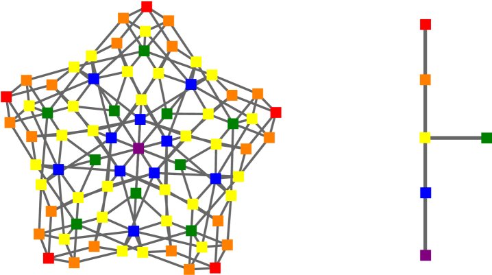
Figure 2. Adjacency graph of the maximal cones of the GIT-fan of $\mathbb{G}(2,5)$ and of their orbits under the $S_{5}$-action.

6. The Mori chamber decomposition of $\operatorname{Mov}(\overline{M}_{0,6})$

In this section, we give a computational proof of Theorem 1.1, that is, we determine the Mori chamber decomposition of the cone of movable divisor classes $\operatorname{Mov}(\overline{M}_{0,6})$ using Algorithm 4.5. The input for the algorithm is the presentation of the Cox ring of $\overline{M}_{0,6}$ in terms of generators and relations determined by Bernal in [4, Theorem 5.4.1] together with the natural $S_{6}$-action thereon. We summarize how to obtain this data in Construction 6.1 and Algorithm 6.3.

Construction 6.1 ($S_{6}$-action on the polynomial ring, see [4, Chapter 5.3]).

Consider the effectively $\mathbb{Z}^{16}$-graded polynomial ring $R$ with $40$ variables

$$R :=\mathbb{K}[y_{1234},y_{1235},y_{1236},y_{1324},y_{1325},y_{1326},y_{1423},y_{1425},y_{1426},y_{1523},y_{1524},y_{1526},y_{1623},$$

$$\phantom{=\mathbb{K}[}\ y_{1624},y_{1625},x_{12},x_{13},x_{14},x_{15},x_{16},x_{23},x_{24},x_{25},x_{26},x_{34},x_{35},x_{36},x_{45},x_{46},x_{56},$$

$$\phantom{=\mathbb{K}\ [}z_{123},z_{124},z_{125},z_{126},z_{134},z_{135},z_{136},z_{145},z_{146},z_{156}]$$

where the grading is given by providing the degrees of the generators $y_{abij}$, $x_{kl}$, $z_{mno}$ as columns of the integral $16\times 40$ matrix

$Q:=$ $\left[\begin{array}[c]{rrrrrrrrrrrrrrr}1&1&1&1&1&1&1&1&1&1&1&1&1&1&1\\ 1&1&1&1&1&1&1&1&1&1&1&1&1&1&1\\ 1&1&1&1&1&1&1&1&1&1&1&1&1&1&1\\ 1&1&1&1&1&1&1&1&1&1&1&1&1&1&1\\ 1&1&1&1&1&1&1&1&1&1&1&1&1&1&1\\ 1&1&1&1&1&1&1&1&1&1&1&1&1&1&1\\ 0&0&0&0&0&0&0&-1&-1&0&-1&-1&0&-1&-1\\ 0&0&0&0&-1&-1&0&0&0&-1&0&-1&-1&0&-1\\ 0&0&0&-1&0&-1&-1&0&-1&0&0&0&-1&-1&0\\ 0&0&0&-1&-1&0&-1&-1&0&-1&-1&0&0&0&0\\ 0&-1&-1&0&0&0&0&0&0&-1&-1&0&-1&-1&0\\ -1&0&-1&0&0&0&-1&-1&0&0&0&0&-1&0&-1\\ -1&-1&0&0&0&0&-1&0&-1&-1&0&-1&0&0&0\\ -1&-1&0&-1&-1&0&0&0&0&0&0&0&0&-1&-1\\ -1&0&-1&-1&0&-1&0&0&0&0&-1&-1&0&0&0\\ 0&-1&-1&0&-1&-1&0&-1&-1&0&0&0&0&0&0\end{array}\begin{array}[c]{|rrrrrrrrrrrrrrr}1&1&1&1&1&0&0&0&0&0&0&0&0&0&0\\ 1&0&0&0&0&1&1&1&1&0&0&0&0&0&0\\ 0&1&0&0&0&1&0&0&0&1&1&1&0&0&0\\ 0&0&1&0&0&0&1&0&0&1&0&0&1&1&0\\ 0&0&0&1&0&0&0&1&0&0&1&0&1&0&1\\ 0&0&0&0&1&0&0&0&1&0&0&1&0&1&1\\ -1&-1&0&0&0&-1&0&0&0&0&0&0&0&0&0\\ -1&0&-1&0&0&0&-1&0&0&0&0&0&0&0&0\\ -1&0&0&-1&0&0&0&-1&0&0&0&0&0&0&0\\ -1&0&0&0&-1&0&0&0&-1&0&0&0&0&0&0\\ 0&-1&-1&0&0&0&0&0&0&-1&0&0&0&0&0\\ 0&-1&0&-1&0&0&0&0&0&0&-1&0&0&0&0\\ 0&-1&0&0&-1&0&0&0&0&0&0&-1&0&0&0\\ 0&0&-1&-1&0&0&0&0&0&0&0&0&-1&0&0\\ 0&0&-1&0&-1&0&0&0&0&0&0&0&0&-1&0\\ 0&0&0&-1&-1&0&0&0&0&0&0&0&0&0&-1\end{array}\begin{array}[c]{|c}\\ \\ 0_{6\times 10}\\ \\ \\ \\ \hline\cr\\ \\ \\ \\ \\ E_{10}\\ \\ \\ \\ \\ \end{array}\right]$

where we denote by $E_{10}$ the $10\times 10$ unit matrix and by $0_{6\times 10}$ the $6\times 10$ zero matrix. Moreover, consider the subgroup $G\subseteq S_{40}$ isomorphic to $S_{6}$ generated by the permutations

$$\sigma_{1} =(4,7)(5,10)(6,13)(8,11)(9,14)(12,15)(17,21)(18,22)(19,23)(20,24)(35,40)(36,39)(37,38),$$

$$\sigma_{2} =(1,4)(2,5)(3,6)(8,9)(11,12)(14,15)(16,17)(22,25)(23,26)(24,27)(32,35)(33,36)(34,37),$$

$$\sigma_{3} =(2,3)(4,7)(5,8)(6,9)(10,11)(13,14)(17,18)(21,22)(26,28)(27,29)(31,32)(36,38)(37,39),$$

$$\sigma_{4} =(1,2)(4,5)(7,10)(8,11)(9,12)(14,15)(18,19)(22,23)(25,26)(29,30)(32,33)(35,36)(39,40),$$

$$\sigma_{5} =(2,3)(5,6)(8,9)(10,13)(11,14)(12,15)(19,20)(23,24)(26,27)(28,29)(33,34)(36,37)(38,39).$$

We then have an action of $G$ on $R$

$$G\times R\,\to\,R,\qquad\sigma_{i}\cdot T_{j}\,:=\,c_{\sigma_{i},j}T_{\sigma(j)}$$

where $T_{j}$ denotes the $j$-th variable of $R$ and the constants $c_{\sigma_{i},j}$ are the entries of the following vectors $c_{\sigma_{i}}\in(\mathbb{K}^{*})^{40}$:

$$c_{\sigma_{1}}$$ ,

,

,

,

.

Here, we write $a^{b}$ for the $b$-fold repetition of $a$.

From the data given by Construction 6.1, Algorithm 6.3 determines an explicit presentation $R/I$ of the Cox ring $\operatorname{Cox}(\overline{M}_{0,6})$.

Proposition 6.2 (Cox ring of $\overline{M}_{0,6}$).

See [4, Chapter 5.4]. In the setting of Construction 6.1, the Cox ring of $\overline{M}_{0,6}$ is isomorphic to $R/\mathfrak{a}$ where

$$\mathfrak{a}\,:=\,(I_{1}+G\cdot I_{2}):(y_{1234}\cdots z_{156})^{\infty},$$

the $\mathbb{Z}^{16}$-degrees of the variables are the respective columns of the matrix $Q$ and the ideals $I_{1},I_{2}\subseteq R$ are defined as follows:

$$I_{1}\ :=\ \langle x_{ij}x_{kl}z_{ijn}z_{kln}-x_{ik}x_{jl}z_{ikn}z_{jln}+x_{il}x_{jk}z_{iln}z_{jkn}\mid\,(i,j,k,l,m,n)\in\mathcal{M}\rangle,$$

$$\mathcal{M}\ :=\ \{ \left(1,2,3,4,5,6\right),\left(1,2,3,5,4,6\right),\left(1,2,3,6,4,5\right),$$

$$\hskip 28.45274pt\left(1,2,4,5,3,6\right),\left(1,2,4,6,3,5\right),\left(1,2,5,6,3,4\right)\},$$

$$I_{2}\ \hphantom{:}=\ \langle z_{126}y_{1423}-x_{13}x_{25}x_{46}z_{123}z_{134}z_{146}+x_{15}x_{24}x_{36}z_{124}z_{145}z_{156},$$

$$z_{126}y_{1425}+x_{13}x_{24}x_{56}z_{124}z_{134}z_{136}-x_{15}x_{23}x_{46}z_{125}z_{145}z_{146},$$

$$z_{125}y_{1426}-x_{13}x_{24}x_{56}z_{124}z_{134}z_{135}-x_{16}x_{23}x_{45}z_{126}z_{145}z_{146},$$

$$z_{126}y_{1523}-x_{13}x_{24}x_{56}z_{123}z_{135}z_{156}+x_{14}x_{25}x_{36}z_{125}z_{145}z_{146},$$

$$z_{126}y_{1524}+x_{13}x_{25}x_{46}z_{125}z_{135}z_{136}-x_{14}x_{23}x_{56}z_{124}z_{145}z_{156},$$

$$z_{124}y_{1526}-x_{13}x_{25}x_{46}z_{125}z_{134}z_{135}+x_{16}x_{23}x_{45}z_{126}z_{145}z_{156},$$

$$z_{125}y_{1623}+x_{13}x_{24}x_{56}z_{123}z_{136}z_{156}+x_{14}x_{26}x_{35}z_{126}z_{145}z_{146},$$

$$z_{125}y_{1624}+x_{13}x_{26}x_{45}z_{126}z_{135}z_{136}+x_{14}x_{23}x_{56}z_{124}z_{146}z_{156},$$

$$z_{135}y_{1625}+x_{12}x_{36}x_{45}z_{125}z_{126}z_{136}-x_{14}x_{23}x_{56}z_{134}z_{146}z_{156},$$

$$x_{12}y_{1234}+x_{13}x_{14}x_{25}x_{26}(z_{134})^{2}-x_{15}x_{16}x_{23}x_{24}(z_{156})^{2},$$

$$x_{12}y_{1235}+x_{13}x_{15}x_{24}x_{26}(z_{135})^{2}-x_{14}x_{16}x_{23}x_{25}(z_{146})^{2},$$

$$x_{12}y_{1236}-x_{13}x_{16}x_{24}x_{25}(z_{136})^{2}+x_{14}x_{15}x_{23}x_{26}(z_{145})^{2},$$

$$x_{13}y_{1324}+x_{12}x_{14}x_{35}x_{36}(z_{124})^{2}+x_{15}x_{16}x_{23}x_{34}(z_{156})^{2},$$

$$x_{13}y_{1325}+x_{12}x_{15}x_{34}x_{36}(z_{125})^{2}+x_{14}x_{16}x_{23}x_{35}(z_{146})^{2},$$

$$x_{13}y_{1326}+x_{12}x_{16}x_{34}x_{35}(z_{126})^{2}+x_{14}x_{15}x_{23}x_{36}(z_{145})^{2}\rangle.$$

Remark 6.3.

In order to make the computation of generators for the ideal $\mathfrak{a}\subseteq R$ in Proposition 6.2 feasible, Bernal [4] proposes to compute the saturation in two steps: saturate the ideals $I_{1}$ and $I_{2}$ separately before saturating their sum.

We can now directly use the results from the previous sections to compute the Mori chamber decomposition of $\overline{M}_{0,6}$. To simplify the computation, we restrict to cones lying within the moving cone $\operatorname{Mov}(\overline{M}_{0,6})$, i.e., the $16$-dimensional polyhedral cone

$$\operatorname{Mov}(\overline{M}_{0,6})\ =\ \bigcap_{i=1}^{40}\operatorname{cone}(q_{j}\mid j\neq i)\ \subseteq\ \operatorname{Eff}(\overline{M}_{0,6})\ \subseteq\ \mathbb{Q}^{16}$$

where the $q_{i}\in\mathbb{Z}^{16}$ are the columns of the degree matrix $Q$ from Construction 6.1 and the cone $\operatorname{Eff}(\overline{M}_{0,6})$ of effective divisor classes equals $\operatorname{cone}(q_{1},\ldots,q_{r})$. The cone $\operatorname{Mov}(\overline{M}_{0,6})$ has $110$ facets and $128\,745$ rays. It contains the cone $\operatorname{SAmple}(\overline{M}_{0,6})$ of semiample divisor classes.

Remark 6.4.

Recall from [1, Section 3.4] that the moving cone encodes the interesting part of Mori chamber decomposition in the following sense: let $D$ be an effective divisor and let $\lambda$ be the GIT-cone of the Mori chamber decomposition with $[D]\in\lambda^{\circ}$. Setting $X:=\overline{M}_{0,6}$, we obtain a birational map

$$\varphi_{D}\colon X\to X(D)\ :=\ \operatorname{Proj}\left(\Gamma\left(X,\mathcal{A}(D)\right)\right),\qquad\mathcal{A}(D)\ :=\ \bigoplus_{n\in\mathbb{Z}_{\geq 0}}\mathcal{O}_{X}(nD).$$

Then the map $\varphi_{D}$ is a small quasimodification, i.e., an isomorphism between open subsets of codimension at least two, if and only if $[D]\in\operatorname{Mov}(\overline{M}_{0,6})^{\circ}$, a morphism if and only if $[D]\in\operatorname{SAmple}(\overline{M}_{0,6})$ and an isomorphism if and only if $[D]\in\operatorname{Ample}(\overline{M}_{0,6})$.

We are in the process of investigating the feasibility of the computation of the full Mori chamber decomposition.

Computational proof of Theorem 1.1.

This is an application of Algorithm 4.5: as input we use the ideal of relations $\mathfrak{a}\subseteq\mathbb{K}[y,x,z]$ of the Cox ring of $\overline{M}_{0,6}$ as given in Proposition 6.2 together with the corresponding grading matrix $Q$ as well as the symmetry group $G$ from Construction 6.1. To restrict our computation to the cone of movable divisor classes $\sigma:=\operatorname{Mov}(\overline{M}_{0,6})$, we change Algorithm 4.5 slightly by redefining the notion of an interior facet to stand for facets $\eta\preceq\lambda$ of GIT-cones $\lambda$ that meet $\sigma^{\circ}$ non-trivially. This yields the Mori chamber decomposition of $\sigma$.

A distinct set of representatives of the maximal cones and the group action can be found in [7]. The numerical properties stated in the theorem can easily be derived from this data by the corresponding functions provided in gitfan.lib. ∎

We immediately retrieve the following statement on the cone of semiample divisor classes; compare also [11, Section 6].

Corollary 6.5.

The Mori cone of $\overline{M}_{0,6}$ is the polyhedral cone in $\mathbb{Q}^{16}$ generated by the $65$ rays in Table 2. The semiample cone of $\overline{M}_{0,6}$ (which is the dual of the Mori cone) has exactly $65$ facets and $3190$ rays.

Proof.

By definition, the semiample cone is contained in the moving cone. By Theorem 1.1, there is exactly one orbit of GIT-cones of length one. Its unique element is, hence, the semiample cone. ∎

-2 1 0 0 1 -1 1 0 0 0 0 1 1 0 0 0 -2 1 0 1 0 -1 1 0 0 0 1 0 1 0 0 0 -2 1 1 0 0 -1 1 0 0 0 1 1 0 0 0 0 -2 1 1 1 1 -1 0 0 0 0 0 0 0 0 0 0 -1 0 0 0 0 -1 1 0 0 1 0 1 0 0 0 0 -1 0 0 0 0 -1 1 0 0 1 1 0 0 0 0 0 -1 0 0 0 0 -1 1 0 1 0 0 0 1 0 0 0 -1 0 0 0 0 -1 1 0 1 0 1 0 0 0 0 0 -1 0 0 0 0 -1 1 1 0 0 0 0 1 0 0 0 -1 0 0 0 0 -1 1 1 0 0 0 1 0 0 0 0 -1 0 0 0 1 -1 1 0 1 1 0 0 0 0 0 0 -1 0 0 0 1 0 0 0 0 0 0 0 0 0 0 -1 -1 0 0 1 0 -1 1 1 0 1 0 0 0 0 0 0 -1 0 0 1 0 0 0 0 0 0 0 0 0 0 -1 0 -1 0 1 0 0 -1 1 1 1 0 0 0 0 0 0 0 -1 0 1 0 0 0 0 0 0 0 0 0 0 -1 0 0 -1 1 0 0 0 -1 1 0 0 0 0 0 1 0 0 1 -1 1 0 0 0 -1 1 0 0 0 0 0 1 0 1 0 -1 1 0 0 0 -1 1 0 0 0 0 1 0 0 0 1 -1 1 0 0 0 -1 1 0 0 0 0 1 0 1 0 0 -1 1 0 0 0 -1 1 0 0 0 1 0 0 0 1 0 -1 1 0 0 0 -1 1 0 0 0 1 0 0 1 0 0 -1 1 0 0 1 -1 1 0 0 0 0 0 0 1 1 0 -1 1 0 0 1 0 0 -1 0 0 0 0 0 0 0 0 -1 1 0 1 0 -1 1 0 0 0 0 0 0 1 0 1 -1 1 0 1 0 0 0 0 -1 0 0 0 0 0 0 0 -1 1 1 0 0 -1 1 0 0 0 0 0 0 0 1 1 -1 1 1 0 0 0 0 0 0 -1 0 0 0 0 0 0 0 0 -1 0 0 -1 1 0 0 0 0 0 1 1 0 0 0 0 -1 0 0 -1 1 0 0 1 0 0 0 1 0 0 0 0 -1 0 0 -1 1 0 0 1 0 0 1 0 0 0 0 0 -1 0 0 0 1 0 0 0 0 0 0 1 0 0 0 0 -1 0 0 0 1 0 0 0 0 0 1 0 0 0

0 0 -1 0 0 0 1 0 0 1 0 0 0 0 0 0 0 0 0 -1 0 -1 1 0 0 0 0 1 0 0 1 0 0 0 0 -1 0 -1 1 0 1 0 0 0 0 0 1 0 0 0 0 -1 0 -1 1 0 1 0 0 1 0 0 0 0 0 0 0 -1 0 0 1 0 0 0 0 0 0 0 1 0 0 0 0 -1 0 0 1 0 0 0 0 1 0 0 0 0 0 0 0 -1 0 0 1 0 1 0 0 0 0 0 0 0 0 0 0 0 -1 -1 1 0 0 0 1 0 0 0 0 1 0 0 0 0 -1 -1 1 1 0 0 0 0 0 0 0 1 0 0 0 0 -1 -1 1 1 0 0 1 0 0 0 0 0 0 0 0 0 -1 0 1 0 0 0 0 0 0 0 0 1 0 0 0 0 -1 0 1 0 0 0 1 0 0 0 0 0 0 0 0 0 -1 0 1 1 0 0 0 0 0 0 0 0 0 0 0 0 0 -1 0 0 0 0 0 0 0 0 0 0 0 0 0 0 0 -1 1 0 0 1 0 0 0 0 0 1 0 0 0 0 0 -1 1 0 0 1 0 0 0 0 1 0 0 0 0 0 0 -1 1 0 1 0 0 0 0 0 0 1 0 0 0 0 0 -1 1 0 1 0 0 0 0 1 0 0 0 0 0 0 0 -1 1 1 0 0 0 0 0 0 1 0 0 0 0 0 0 -1 1 1 0 0 0 0 0 1 0 0 0 0 0 0 0 0 0 -1 0 0 0 0 0 0 0 0 0 0 0 0 0 0 0 0 -1 0 0 0 0 0 0 0 0 0 0 0 0 0 0 0 0 -1 0 0 0 0 0 0 0 0 0 0 0 0 0 0 0 0 -1 0 0 0 0 0 0 0 0 0 0 0 0 0 0 0 0 -1 0 0 0 0 0 0 0 0 0 0 0 0 0 0 0 0 -1 0 0 0 0 0 0 0 0 0 0 0 0 0 0 0 0 -1 0 0 0 0 0 0 0 0 0 0 0 0 0 0 0 0 -1 0 0 0 0 0 0 0 0 0 0 0 0 0 0 0 0 -1 0 0 0 0 1 0 0 0 0 0 -1 0 0 0 0 0 0 0 0 1 0 0 0 0 0 0 0 -1 0 0 0 0 0 0 1 0 0 0 0 0 0 0 0 0 -1 0 0 0

Table 2. Extremal rays of the Mori cone of $\overline{M}_{0,6}$, specified as rows.

Remark 6.6.

The set of minimal orbit cones of dimension $16$ intersected with the moving cone is the union of two distinct orbits consisting of $45$ elements each.

Remark 6.7.

As suggested by Diane Maclagan, one may expect that the restriction of the GIT-fan to $\operatorname{Mov}(\overline{M}_{0,6})$ can also be obtained by restricting to the subring

$$\mathbb{K}[x_{12},x_{13},x_{14},x_{15},x_{16},x_{23},x_{24},x_{25},x_{26},x_{34},x_{35},x_{36},x_{45},x_{46},x_{56},$$

$$\phantom{\mathbb{K}\ [}z_{123},z_{124},z_{125},z_{126},z_{134},z_{135},z_{136},z_{145},z_{146},z_{156}]$$

of $R$, i.e., by eliminating the variables corresponding to the Keel-Vermeire divisors from the ideal $\mathfrak{a}$ (constructed in Proposition 6.2). The corresponding computation shows that the set of minimal orbit cones of dimension $16$ intersected with the moving cone is the union of three distinct orbits, two of length $45$, which agree with those mentioned in Remark 6.6, and one of length $15$. Each cone in the orbit of length $15$ is the intersection of three cones in one of the orbits of length $45$, hence, the resulting Mori chamber decomposition of $\operatorname{Mov}(\overline{M}_{0,6})$ agrees with that in Theorem 1.1.

Remark 6.8.

The computations for the proof of Theorem 1.1 took approximately $8$ days, about one week for obtaining the $\mathfrak{a}$-faces (with a parallel computation on 16 cores) and one day for deriving the GIT-cones (by a parallel fan traversal on $16$ cores). Making use of the group action of $G$, representing GIT-cones via the hash function of Construction 4.3, and applying Algorithm 3.3 for the monomial containment tests turned out to be crucial for finishing the computation.

References

• [1] I. Arzhantsev, U. Derenthal, J. Hausen, and A. Laface. Cox rings, volume 144 of Cambridge Studies in Advanced Mathematics. Cambridge University Press, Cambridge, 2014.
• [2] I. V. Arzhantsev and J. Hausen. Geometric invariant theory via Cox rings. J. Pure Appl. Algebra, 213(1):154–172, 2009.
• [3] F. Berchtold and J. Hausen. GIT equivalence beyond the ample cone. Michigan Math. J., 54(3):483–515, 2006.
• [4] M. M. Bernal Guillén. Relations in the Cox Ring of $\overline{M}_{0,6}$. PhD thesis, University of Warwick, 2012.
• [5] J. Böhm, W. Decker, S. Keicher, and Y. Ren. Current challenges in developing open source computer algebra systems. In Mathematical aspects of computer and information sciences. 6th international conference, MACIS 2015, Berlin, Germany, November 11–13, 2015. Revised selected papers, pages 3–24. Cham: Springer, 2016.
• [6] J. Böhm, S. Keicher, and Y. Ren. gitfan.lib – A Singular library for computing the GIT fan, 2016. Available in the Singular distribution, https://github.com/Singular/Sources.
• [7] J. Böhm, S. Keicher, and Y. Ren. The Mori Chamber Decomposition of the Movable Cone of $\overline{M}_{0,6}$, 2016. Online data available at http://www.mathematik.uni-kl.de/~boehm/gitfan.
• [8] A.-M. Castravet. The Cox ring of $\overline{M}_{0,6}$. Trans. Amer. Math. Soc., 361(7):3851–3878, 2009.
• [9] W. Decker, G.-M. Greuel, G. Pfister, and H. Schönemann. Singular 4-0-2 — A computer algebra system for polynomial computations. http://www.singular.uni-kl.de, 2014.
• [10] I. V. Dolgachev and Y. Hu. Variation of geometric invariant theory quotients. Inst. Hautes Études Sci. Publ. Math., (87):5–56, 1998. With an appendix by Nicolas Ressayre.
• [11] A. Gibney and D. Maclagan. Lower and upper bounds for nef cones. Int. Math. Res. Not. IMRN, (14):3224–3255, 2012.
• [12] B. Hassett and Y. Tschinkel. On the effective cone of the moduli space of pointed rational curves. In Topology and geometry: commemorating SISTAG, volume 314 of Contemp. Math., pages 83–96. Amer. Math. Soc., Providence, RI, 2002.
• [13] J. Hausen, S. Keicher, and R. Wolf. Computing automorphisms of Mori dream spaces. 2015. Preprint. See arXiv:1511.05059.
• [14] Y. Hu and S. Keel. Mori dream spaces and GIT. Michigan Math. J., 48:331–348, 2000. Dedicated to William Fulton on the occasion of his 60th birthday.
• [15] S. Keicher. Computing the GIT-fan. Internat. J. Algebra Comput., 22(7):1250064, 11, 2012.
• [16] D. Mumford, J. Fogarty, and F. Kirwan. Geometric invariant theory, volume 34 of Ergebnisse der Mathematik und ihrer Grenzgebiete (2) [Results in Mathematics and Related Areas (2)]. Springer-Verlag, Berlin, third edition, 1994.
• [17] B. Sturmfels. Gröbner bases and convex polytopes, volume 8 of University Lecture Series. American Mathematical Society, Providence, RI, 1996.
• [18] M. Thaddeus. Geometric invariant theory and flips. J. Amer. Math. Soc., 9(3):691–723, 1996.