March 2016

We investigated regular black holes with fuzzy sources in three and four dimensions. The density distributions of such fuzzy sources are inspired by noncommutative geometry and given by Gaussian or generalized Gaussian functions. We utilized mass functions to give a physical interpretation of the horizon formation condition for the black holes. In particular, we investigated three-dimensional BTZ-like black holes and four-dimensional Schwarzschild-like black holes in detail, and found that the number of horizons is related to the spacetime dimensions, and the existence of a void in the vicinity of the center of the spacetime is significant, rather than noncommutativity. As an application, we considered a three-dimensional black hole with the fuzzy disc which is a disc-shaped region known in the context of noncommutative geometry as a source. We also analyzed a four-dimensional black hole with a source whose density distribution is an extension of the fuzzy disc, and investigated the horizon formation condition for it.

1 Introduction

Quantum features of spacetime have been discussed for a long time and there have been so many trials to depict their physics. Instead of enthusiastic studies, we still do not know which manner can be the most natural criterion to quantize a spacetime. Consequently, our starting point is to investigate such a phenomenon that definitely appears when a spacetime is consistently quantized. Spacetime noncommutativity is one of such features, even though there might be diverse ways to impose noncommutativity[1, 2, 3, 4, 5]. We can naively expect that noncommutativity makes various changes in the structures of spacetimes, in particular, black hole spacetimes and the very early universe.

In this context, the authors of [6] investigated a four-dimensional spacetime with a source inspired by noncommutative geometry. As a consequence of noncommutativity, they proposed a source that has a Gaussian distribution $e^{-r^{2}/(2\theta)}$ instead of a delta function $\delta^{(3)}(\mbox{\boldmath$r$})$ since we have to abandon a picture of zero size object like a point particle and should replace it by something smeared. Here $\theta$ is a noncommutative parameter that represents spacetime noncommutativity, e.g., $[x,y]=i\theta$ in a two-dimensional space. They found that there can exist a black hole with such a source at its center. It is a regular black hole in the sense that the curvature singularity at the center is resolved since the matter source is diffused by noncommutativity. What we want to focus on here about the black hole in [6] is that it can have two horizons as long as an appropriate condition is satisfied, even though it is not charged, nor does it have an angular momentum. The existence of a black hole with two horizons means that there would be an extreme black hole where two horizons coincide and there would appear a remnant after the Hawking radiation starting from a non-extreme black hole. This may change a story of the black hole evaporation. Inspired by this fascinating scenario, a lot of works on black holes with such Gaussian sources have been done so far [7, 8, 9, 10, 11, 12, 13, 14, 15].

One more thing we want to note is that there is always a solution for any density distribution because the corresponding energy-momentum tensor of anisotropic fluid compensates for a consistent solution to exist. This is another reason that many authors have been able to consider these noncommutative geometry inspired black holes, which also has been referred in the context of another type of regular black holes [16, 17, 18].

It is thereby natural that this research has been extended to three-dimensional black holes. Though a three-dimensional spacetime is intrinsically different from a four-dimensional spacetime, as is well known, there exists the BTZ black hole in a three-dimensional spacetime with a negative cosmological constant. The authors of [19, 20, 21, 22, 23] analyzed three-dimensional black holes with Gaussian sources which have similar structures to the BTZ black hole, in the sense that the spacetimes are asymptotically anti de Sitter, but at the same time, there are de Sitter cores around the centers on the contrary to the BTZ black hole. As we will see later, there is no black hole with two horizons due to the core [23]. Motivated by this fact, the authors of [23] and [24] introduced generalized Gaussian sources whose density distributions are proportional to $re^{-r^{2}/(2\theta)}$ and $r^{2}e^{-r^{2}/(2\theta)}$, respectively. The change of sources makes a black hole have two horizons as long as an appropriate condition is satisfied.

The aim of this paper is to clarify what is physically essential for a spacetime with such a fuzzy source to have a horizon. In particular, we are interested in how noncommutativity changes the number of horizons. Here we want to move away from the specifics and consider general properties. To this end, we utilize a mass function that denotes the mass within a given radius. Such a mass function determines the condition for a spacetime to have a horizon, since the necessary mass that must be included within the horizon radius is automatically determined, once the radius of a black hole is given.

In the rest of this paper, we will investigate the existence of horizons and the number of them for a three-dimensional black hole with a source described by a generalized Gaussian $r^{n}e^{-r^{2}/(2\theta)}$, using a mass function and a characteristic function which denotes the horizon formation condition. In order to do so, we will solve the Einstein equation with anisotropic fluid corresponding to the source and the negative cosmological constant. Also, we will see that, for a three-dimensional black hole, the existence of a void around its center is crucial to have two horizons. We use a toy model whose density distribution is not related to noncommutativity to check our statement.

Since the characteristic function we will propose here to judge the horizon formation is intuitive and graphically versatile, we can apply it to various cases. In fact, we consider a three-dimensional black hole with a source whose density distribution is originally motivated by the fuzzy disc in noncommutative geometry. The fuzzy disc is a disc-shaped region in a two-dimensional Moyal plane and its corresponding function is a sum of density distributions represented by the generalized Gaussian functions. We will also investigate an extension of the density distribution of the fuzzy disc type and a black hole around it in a four-dimensional spacetime.

This paper is organized as follows. In Sec.2, we show how a mass function is used to determine the horizon formation condition, using the Reissner-Nortstrøm black hole as an example, and we apply the same manner to the four-dimensional black hole argued in [6]. In Sec.3, we will analyze three-dimensional black holes with fuzzy sources whose density distributions are given by the generalized Gaussian functions. We will investigate the characteristic function for the horizon formation condition in detail, and will see what is essential for a horizon to be formed. In Sec.4, noncommutative geometry inspired black holes with sources motivated from the fuzzy disc are considered. Sec.5 is devoted to conclusion and discussion. We also refer a black hole spacetime with multi-horizon and the fuzzy annulus as its source.

2 Mass function and horizon formation condition

The existence of a black hole, in other words, the existence of a horizon, depends on how much mass is condensed in a given region. Even if there is a large amount of mass, but it is too diffused, a black hole horizon can not be formed. Since the sources we will treat in this paper are smeared by replacing the delta function to the Gaussian functions, how much mass exists within a given radius is essential for a spacetime to have a horizon. A mass function is intuitively useful to express such a necessary mass.

2.1 Reissner-Nortstrøm black hole and horizon formation condition

In order to judge when a horizon is formed for a noncommutative geometry inspired black hole, we can utilize a mass function. It is the profile of the mass distribution that is calculated by the volume integration of a density. It also can be regarded as an effective mass that is obtained by an analogue to the Schwarzschild mass. For example, let us consider the Reissner-Nortstrøm (RN) solution. In $G=c=1$ unit, the line element of the four-dimensional RN black hole is given by

$$ds^{2}=-\left(1-\frac{2M}{r}+\frac{Q^{2}}{r^{2}}\right)dt^{2}+\left(1-\frac{2M}{r}+\frac{Q^{2}}{r^{2}}\right)^{-1}dr^{2}+r^{2}d\Omega_{(2)}^{2},$$ (2.1)

where $M$ is the total mass in the spacetime, and $Q$ is the electric charge of the black hole. The existence of a horizon is determined by the divergent behavior of the $(rr)$-component of the metric. In other words, the number of roots for the equation

$$f(r)=1-\frac{2M}{r}+\frac{Q^{2}}{r^{2}}=0,$$ (2.2)

corresponds to the number of the horizons. If $M>|Q|$, the RN metric describes the black hole spacetime with two horizons. They are located at $r_{\pm}=M\pm\sqrt{M^{2}-Q^{2}}$. If $M=|Q|$, there is a special type of a black hole with one horizon. This is an extreme RN black hole in which $r_{+}$ and $r_{-}$ coincide. If $M<|Q|$, there is no black hole, but a naked singularity that does not have a horizon.

We can graphically clarify if a horizon exists or not by introducing a mass function. The mass function $m(r)$ for the RN black hole is defined as

$$m(r)=M-\frac{Q^{2}}{2r}.$$ (2.3)

Using $m(r)$, the line element of the RN black hole is rewritten as

$$ds^{2}=-\left(1-\frac{2m(r)}{r}\right)dt^{2}+\left(1-\frac{2m(r)}{r}\right)^{-1}dr^{2}+r^{2}d\Omega_{(2)}^{2},$$ (2.4)

which can be regarded as the line element of the Schwarzschild black hole with the effective mass $m(r)$. Eq.(2.2) is also rewritten as

$$f(r)=1-\frac{2m(r)}{r}=0,$$ (2.5)

which gives the horizon formation condition.

One of the advantages of this perspective is that it enables us to understand why an infalling observer can avoid hitting the singularity at the center of the RN black hole. Actually, inside the inner horizon ($0\leq r\leq r_{-}$), the mass function is always negative, which makes the gravitational force effectively repulsive there [25].

Another advantage of introducing the mass function, which will become more significant in the following analyses in this paper, is that it makes us possible to argue the horizon formation condition based on the analogue of a well-known black hole. Though there is no geometrical basis to define a mass function, we can choose a simpler and more useful one for a spacetime we want to consider. Clearly, for four-dimensional regular black holes, we can use the Schwarzschild black hole as such. The Schwarzschild horizon depends on its mass as

$$r_{h}=2M,$$ (2.6)

which means that if there is a Schwarzschild black hole with radius $r_{h}$, the total mass $M_{h}=r_{h}/2$ must be included within radius $r_{h}$. More precisely, if a mass included inside a sphere of radius $r_{h}$ is equal to or larger than $r_{h}/2$, a black hole is formed.

Applying this idea to the RN case, we can interpret the horizon formation condition using the mass function as the existence of $r_{h}$ that satisfies

$$m(r_{h})\geq M_{h}=\frac{r_{h}}{2}.$$ (2.7)

This condition states that once a horizon radius is given, the total mass that must be included within the radius will be determined automatically. Of course, this condition obviously coincide with $f(r)=0$, but our point of view is physically more apparent. For the RN case, the condition for a horizon to be formed can be rewritten as

$$M-\frac{Q^{2}}{2r_{h}}\geq\frac{r_{h}}{2}\quad\Leftrightarrow\quad\frac{1}{M}\leq\frac{2r_{h}}{r_{h}^{2}+Q^{2}}.$$ (2.8)

The existence of a horizon is determined by the number of intersections between the following characteristic function

$$h(x)=\displaystyle\frac{2x}{x^{2}+q^{2}},$$ (2.9)

and the constant function that represents the value of $L/M$. Here $L$ is a typical length of this spacetime, which is introduced to define dimensionless parameters $L/M$, $x\equiv r_{h}/L$ and $q\equiv Q/L$. Now the condition (2.8) is translated to

$$\frac{L}{M}\leq h(x)=\displaystyle\frac{2x}{x^{2}+q^{2}}.$$ (2.10)

The profile of $h(x)$ is shown in Fig.1.

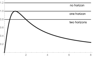
Figure 1: Plot of $h(x)$ with $q=1$ defined in (2.9). The horizontal lines denote the values of $L/M$. The number of intersections corresponds to the numbers of horizons.

By the way, we are writing the condition for the inverse of mass $1/M$, not for $M$. This is because $h(x)$ does not diverge both around $x=0$ and for $x\to\infty$, which makes it simpler to analyze the behavior of the horizon formation condition around $x=0$ and $x\to\infty$. This usage of the mass function have not been seen in the previous works.

The characteristic function $h(x)$ takes its maximum value $1/q$ at $x=q$. $L/M$ must therefore be equal to or smaller than $1/q$ in order that at least one horizon exists. When $M=Q\ (\Leftrightarrow L/M=1/q)$, there is one horizon, which corresponds to the extreme black hole. For $M>Q$, there are two horizons. These facts on the RN black hole are well known.

We will investigate the horizon formation conditions for various sources in the same manner in the rest of this paper. As mentioned before, there is no generally natural definition of a mass function for an arbitrary spacetime, and we can use an suitable form for a spacetime we want to consider. In fact, we will consider an analogue of the BTZ black hole to define a mass function in three dimensions, on the contrary to the Schwarzschild black hole in four dimensions.

2.2 Horizon formation condition for a four-dimensional noncommutative geometry inspired Schwarzschild black hole

We want to apply the method in the previous subsection to investigate the horizon formation condition for a four-dimensional regular black hole inspired by noncommutative geometry considered in [6]. The density distribution of the source of the black hole has a Gaussian shape $\rho(r)\propto e^{-r^{2}/(2\theta)}$. Here $\theta$ is a noncommutative parameter that defines the canonical commutation relation between space coordinates as

$$[x,y]=i\theta.$$ (2.11)

When this relation is imposed to a space, we can naively expect that there is no ‘zero-size’ object. For example, a source of the delta function type would be smeared and fuzzy. Then one of the simplest realizations is to replace the delta function to a Gaussian function

$$\delta^{(3)}(\mbox{\boldmath$r$})\to\exp\left(-\frac{r^{2}}{2\theta}\right).$$ (2.12)

The authors of [6] made use of the fact that for any density distribution, there exist the corresponding solution for the Einstein equation because of compensating by an appropriate component of the energy-momentum tensor of anisotropic fluid. In [6], the tangential pressure $T_{\phi\phi}$ plays the role. This has been extend to various black holes, e.g., charged [7], rotating [11, 12], or lower-dimensional [14] and higher-dimensional ones [26], and so on. The reference [13] is a review of noncommutative geometry inspired black holes written by one of the authors of [6].

The solution shown in [6] is given by

$$ds^{2}=-\left(1-\frac{2m_{4d}(r)}{r}\right)dt^{2}+\left(1-\frac{2m_{4d}(r)}{r}\right)^{-1}dr^{2}+r^{2}\left(d\theta^{2}+\sin^{2}\theta d\phi^{2}\right),$$ (2.13)

where

$$m_{4d}(r) = 4\pi\int_{0}^{r}dr^{\prime}r^{\prime 2}\rho_{4d}(r^{\prime})=4\pi\int_{0}^{r}dr^{\prime}r^{\prime 2}\frac{M}{(2\pi\theta)^{3/2}}\exp\left(-\frac{r^{\prime 2}}{2\theta}\right)$$ (2.14)

$$= \frac{2M}{\sqrt{\pi}}\gamma\left(\frac{3}{2},\frac{r^{2}}{2\theta}\right),$$

is the mass function for this system. $\gamma(a,x)$ is the lower incomplete gamma function related to the upper incomplete gamma function as

$$\gamma(a,x)=\Gamma(a)-\Gamma(a,x).$$ (2.17)

The normalization is determined by $m_{4d}(r=\infty)=M$, which gives the total mass in the whole space.

Repeating the same argument for the RN black hole, we can interpret the horizon formation condition as the existence of $r_{h}$ that satisfies

$$m_{4d}(r_{h})\geq M_{h}=\frac{r_{h}}{2}\quad\Leftrightarrow\quad\frac{2M}{\sqrt{\pi}}\gamma\left(\frac{3}{2},\frac{r^{2}}{2\theta}\right)\geq\frac{r_{h}}{2}.$$ (2.18)

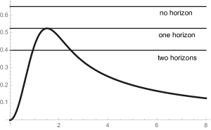
Figure 2: Plot of $h_{4d}(x)$. The horizontal lines denote the values of $\sqrt{2\theta}/M$. $h_{4d}(x)$ takes the maximum value $h_{4d}^{*}=0.525$ at $x=1.51$. When $M>\sqrt{2\theta}/h_{4d}^{*}$, there are two horizons. When $M=\sqrt{2\theta}/h_{4d}^{*}$, there is one horizon, which corresponds to the extreme black hole. When $M<\sqrt{2\theta}/h_{4d}^{*}$, there is no horizon, which means that no black hole is formed but a regular lump of mass like a star exists.

Introducing a dimensionless parameter $x=r_{h}/\sqrt{2\theta}$, the condition is interpreted as the existence of $x$ that satisfies

$$h_{4d}(x)\equiv\frac{2\gamma\left(\frac{3}{2},x^{2}\right)}{\sqrt{\pi}x}\geq\frac{\sqrt{2\theta}}{M}.$$ (2.19)

The plot of $h_{4d}(x)$ is shown in Fig.2. $h_{4d}(x)$ takes the maximum value $\thickapprox 0.525$ at $x=1.51$, which means that the extreme black hole exists when

$$M\thickapprox\frac{\sqrt{2\theta}}{0.525}.$$ (2.20)

For $M$ which is larger than $\sqrt{2\theta}/0.525$, there is a black hole with two horizons. This result coincides with [6], multiplying two to $\theta$ to replace the noncommutative parameter used in [6].

3 Three-dimensional black hole with fuzzy source

3.1 Three-dimensional rotating regular black hole with anisotropic fluid

We can easily extend the analysis in the previous section to three-dimensional cases. To begin with, let us show that there is a black hole which corresponds to any density distribution $\rho(r)$ also in three dimensions.

	$n$	$Q$	$J$	$\Lambda$
Rahaman et al. [19]	$\quad\ \quad 0\quad\ \quad$	$\quad\ \quad 0\quad\ \quad$	$\quad\ \quad 0\quad\ \quad$	$\quad\ \quad<0\quad\ \quad$
Tejeiro & Larranaga [20]	0	0		$<0$
Tejeiro & Larranaga [21]	0	$\propto e^{-r^{2}/(4\theta)}$	0	$<0$
Rahaman et al [22]	0	$\propto r^{n+2}$	0	$<0$
Myung & Yoon [23]	0, 1	0	0	$<0$
Liang, Liu & Zhu [24]	2	0		$<0$
Park [27]	$n$	0	0	$>0$

Table 1: Three-dimensional black holes with fuzzy sources

As summarized in Table.1, various types of three-dimensional, noncommutative geometry inspired black holes have been proposed so far. All of them were modifications of the BTZ black hole by replacing densities of the delta function type to the Gaussian type

$$\rho(r)\propto e^{-\frac{r^{2}}{2\theta}},$$ (3.1)

or the generalized Gaussian type

$$\rho(r)\propto r^{n}e^{-\frac{r^{2}}{2\theta}}\quad(n\geq 1).$$ (3.2)

To consider a concrete spacetime, we first derive a three-dimensional, circular symmetric solution of the Einstein equation with the negative cosmological constant

$$G_{\mbox{}\ \nu}^{\mu}=8\pi T_{\mbox{}\ \nu}^{\mu}+\Lambda\delta_{\mbox{}\ \nu}^{\mu}.$$ (3.3)

$\Lambda$ is the cosmological constant which is related to the curvature length $\ell$ as $\Lambda=-1/\ell^{2}$. In this paper we use $c=G_{3}=1$ unit, where $G_{3}$ is the three-dimensional gravitational constant.

We want to consider a circular symmetric spacetime described by the following metric

$$ds^{2}=-f(r)dt^{2}+f^{-1}(r)dr^{2}+r^{2}\left[d\phi+N_{\phi}(r)dt\right]^{2}.$$ (3.4)

The spacetime denoted by this metric has an angular momentum that is similar to the BTZ black hole. For the energy-momentum tensor $T_{\mbox{}\ \nu}^{\mu}$, we impose the following ansatz

$$T_{\mbox{}\ t}^{t}=-\rho(r),\quad T_{\mbox{}\ r}^{r}=p_{r}(r),\quad T_{\mbox{}\ \phi}^{\phi}=p_{\phi}(r)$$

$$T_{\mbox{}\ t}^{\phi}=\sigma_{a}(r),\quad T_{\mbox{}\ \phi}^{t}=\sigma_{b}(r),\quad\mbox{others are zero}.$$ (3.6)

When we consider a rotating solution, i.e., $N_{\phi}\neq 0$, the energy-momentum tensor can be no longer diagonal. In fact, we can not set $T_{\mbox{}\ t}^{\phi}=\sigma_{a}(r)=0$ to solve the equations of motion consistently, though $\sigma_{b}$ can be zero as we will see explicitly. This point is not referred in [20] and [24] though the existence of the $(\phi,t)$-component of the energy-momentum tensor does not affect their conclusions. Since $T_{\phi t}$ and $T_{t\phi}$ must be same, we find that $\sigma_{a}$ and $\sigma_{b}$ obey

$$\sigma_{a}=\left(-\frac{f}{r^{2}}+N_{\phi}^{2}\right)\sigma_{b}+N_{\phi}(p_{\phi}+\rho),$$ (3.7)

which can be used to check the consistency.

Now we find that the Einstein equation $G_{\mbox{}\ \nu}^{\mu}=8\pi T_{\mbox{}\ \nu}^{\mu}+\Lambda\delta_{\mbox{}\ \nu}^{\mu}$ reduces to

$$2f^{\prime}+r^{2}[rN_{\phi}^{\prime 2}+2N_{\phi}(3N_{\phi}^{\prime}+rN_{\phi}^{\prime\prime})] = 4r\left(-8\pi\rho+\frac{1}{\ell^{2}}\right),$$ (3.8)

$$2f^{\prime}+r^{3}N_{\phi}^{\prime 2} = 4r\left(8\pi p_{r}+\frac{1}{\ell^{2}}\right),$$ (3.9)

$$-3r^{2}N_{\phi}^{\prime 2}+2f^{\prime\prime}-2N_{\phi}(3N_{\phi}^{\prime}+rN_{\phi}^{\prime\prime}) = 4\left(8\pi p_{\phi}+\frac{1}{\ell^{2}}\right),$$ (3.10)

$$r(3N_{\phi}^{\prime}+rN_{\phi}^{\prime\prime}) = 16\pi\sigma_{b}$$ (3.11)

$$N_{\phi}(f^{\prime}+2r^{3}N_{\phi}^{\prime 2}-rf^{\prime\prime})+(f+r^{2}N_{\phi}^{2})(3N_{\phi}^{\prime}+rN_{\phi}^{\prime\prime}) = -16\pi r\sigma_{a}$$ (3.12)

They are $(t,t),(rr),(\phi\phi),(t,\phi)$ and $(\phi,t)$-components of the Einstein equation, respectively. The prime denotes the derivative with respect to $r$. Besides them, we have to consider the covariant conservation of the energy-momentum tensor $T_{\mbox{}\ \mbox{}\ ;\nu}^{\mu\nu}=0$. For $\mu=r$, it gives a non-trivial equation

$$r\left\{f^{\prime}(p_{r}+\rho)+r^{2}N_{\phi}^{\prime}(\sigma_{a}-N_{\phi}^{2}\sigma_{b})+N_{\phi}\left[\sigma_{b}f^{\prime}-r^{2}(p_{r}+\rho)N_{\phi}^{\prime}\right]\right\}\\ +f(2p_{r}-2p_{\phi}-2N_{\phi}\sigma_{b}-r\sigma_{b}N_{\phi}^{\prime}+2rp^{\prime}_{r})=0.$$ (3.13)

There are six equations (3.8)-(3.13) and one condition (3.7) for the symmetry of the energy-momentum tensor to determine five unknown functions $f,N_{\phi},\sigma_{a},\sigma_{b},p_{r}$ and $p_{\phi}$. In deriving solutions, we will put an ansatz to reduce the totally seven equations into six. The redundant equation among the rest six equations is due to the Bianchi identity.

When we impose a simple ansatz $\sigma_{b}=0$, Eq.(3.11) can easily be integrated as

$$N_{\phi}(r)=-\frac{J}{2r^{2}},$$ (3.14)

which coincides with the BTZ case. $J$ corresponds to the angular momentum of a black hole. Substituting this into the other equations, we see that all the other unknown functions $f,\sigma_{a},p_{r}$ and $p_{\phi}$ are determined as the functions of the energy density $\rho$

$$f(r) = -16\pi\int_{0}^{r}dr^{\prime}\ r^{\prime}\rho(r^{\prime})+\frac{r^{2}}{\ell^{2}}+\frac{J^{2}}{4r^{2}},$$ (3.15)

$$= -8m(r)+\frac{r^{2}}{\ell^{2}}+\frac{J^{2}}{4r^{2}}$$

$$\sigma_{a}(r) = \frac{J}{2r}\rho^{\prime}(r)$$ (3.16)

$$p_{r}(r) = -\rho(r),$$ (3.17)

$$p_{\phi}(r) = -(r\rho(r))^{\prime},$$ (3.18)

where we set an integration constant in $f(r)$ to zero for this solution to coincide with the BTZ black hole for a large $r$. $m(r)$ is the mass function for a given density $\rho$, which is defined by

$$m(r)=2\pi\int dr^{\prime}r^{\prime}\rho(r^{\prime}).$$ (3.19)

The Ricci scalar for this solution in terms of $f$ and $N_{\phi}$ is

$$R=-f^{\prime\prime}(r)-\frac{2}{r}f^{\prime}(r)+\frac{1}{2}r^{2}N_{\phi}^{2}(r).$$ (3.20)

Substituting (3.15) and (3.14) to (3.20), we obtain

$$R=16\pi(3\rho(r)+r\rho^{\prime}(r))-\frac{6}{\ell^{2}}+\frac{J^{2}}{8r^{2}}.$$ (3.21)

The energy-momentum tensor with lower indices is given by

$$(T_{\mu\nu})=\left(\begin{array}[]{ccc}T_{tt}&T_{tr}&T_{t\phi}\\ T_{rt}&T_{rr}&T_{r\phi}\\ T_{\phi t}&T_{\phi r}&T_{\phi\phi}\end{array}\right)=\left(\begin{array}[]{ccc}f\rho+\displaystyle\frac{J}{2}(r\rho)^{\prime}&0&\displaystyle\frac{J}{2}(r\rho)^{\prime}\\ 0&\displaystyle-\frac{\rho}{f}&0\\ \displaystyle\frac{J}{2}(r\rho)^{\prime}&0&-r^{2}(r\rho)^{\prime}\end{array}\right),$$ (3.22)

which is diagonal only for $J=0$ as mentioned before.

3.2 Generalized non-Gaussian sources in three dimensions

We investigate spacetimes with various sources that appear in the context of noncommutative geometry. As an instructive example, let us first see the spacetime with the generalized Gaussian source, $\rho\propto r^{n}e^{-r^{2}/(2\theta)}$. To be more concrete, we consider the following density distribution described by the generalized Gaussian function

$$\rho_{n}(r)=\frac{M}{2\pi\theta(2\theta)^{\frac{n}{2}}\Gamma\left(\frac{n}{2}+1\right)}r^{n}e^{-\frac{r^{2}}{2\theta}}.$$ (3.23)

The corresponding mass function is

$$m_{n}(r) = 2\pi\int_{0}^{r}r^{\prime}\rho(r^{\prime})dr^{\prime}=\frac{M}{\Gamma\left(\frac{n}{2}+1\right)}\gamma\left(\frac{n}{2}+1,\frac{r^{2}}{2\theta}\right)$$ (3.24)

$$= M\left[1-\frac{\Gamma\left(\frac{n}{2}+1,\frac{r^{2}}{2\theta}\right)}{\Gamma\left(\frac{n}{2}+1\right)}\right].$$

Similar to the four-dimensional case, the mass function is normalized as $m_{n}(\infty)=M$ using $\Gamma(\frac{n}{2}+1,\infty)=\Gamma(\frac{n}{2}+1)$. The ratio of $M$ to the noncommutative parameter $\sqrt{2\theta}$ determines the horizon formation condition.

3.3 Black holes with a generalized Gaussian source and physical interpretation of their horizons

Hereafter we set $J=0$ for simplicity, but the essence of our analysis does not depend on it and we can extend this to the case with nonzero $J$. Putting the density distribution (3.23) to (3.18) and setting $J=0$, we obtain

$$ds^{2}=-f_{n}(r)dt^{2}+f_{n}^{-1}(r)dr^{2}+r^{2}d\phi^{2},$$ (3.25)

where

$$f_{n}(r) = -8m_{n}(r)+\frac{r^{2}}{\ell^{2}}$$ (3.26)

$$= \frac{M}{\Gamma(n+1)}\left[\gamma\left(n+1,\frac{r^{2}}{2\theta}\right)+\frac{r^{2}}{2\theta}\gamma\left(n,\frac{r^{2}}{2\theta}\right)\right]+\frac{r^{2}}{\ell^{2}},$$

$$p_{nr}(r) = -\rho_{n}(r)$$ (3.27)

$$= -\frac{M}{2\pi\theta(2\theta)^{\frac{n}{2}}\Gamma\left(\frac{n}{2}+1\right)}r^{n}e^{-\frac{r^{2}}{2\theta}},$$

$$p_{n\phi}(r) = -(r\rho_{n}(r))^{\prime}$$ (3.28)

$$= -\frac{M}{2\pi\theta(2\theta)^{\frac{n}{2}}\Gamma\left(\frac{n}{2}+1\right)}\left(n+1-\frac{r^{2}}{\theta}\right)r^{n}e^{-\frac{r^{2}}{2\theta}}.$$

In order to obtain the physical interpretation of the three-dimensional spacetime described above, let us go back to see the BTZ black hole spacetime. The non-rotating BTZ solution is represented by the following line element

$$ds^{2}=-\left(-8M+\frac{r^{2}}{\ell^{2}}\right)dt^{2}+\left(-8M+\frac{r^{2}}{\ell^{2}}\right)^{-1}dr^{2}+r^{2}d\phi^{2}.$$ (3.29)

The horizon radius is given by

$$r_{h}=\sqrt{8M\ell^{2}},$$ (3.30)

which is determined by $g_{tt}=g_{rr}^{-1}=0$.

As shown in the previous sections, we can see this equation as the condition for the mass that is necessary for a horizon with radius $r_{h}$ to be formed. In this case

$$M=\frac{r_{h}^{2}}{8\ell^{2}},$$ (3.31)

is the necessary mass inside a circle with radius $r_{h}$ for the BTZ black hole to have the horizon. We use this condition to judge whether the three-dimensional black hole with the generalized Gaussian source can have a horizon or not.

For the spacetime described by (3.25)-(3.28), the mass function is calculated as (3.24). The horizon formation condition is thereby interpreted as the existence of $r_{h}$ that satisfies

$$m_{n}(r_{h})=M\left[1-\frac{\Gamma\left(\frac{n}{2}+1,\frac{r_{h}^{2}}{2\theta}\right)}{\Gamma\left(\frac{n}{2}+1\right)}\right]\geq\frac{r_{h}^{2}}{8\ell^{2}},$$ (3.32)

or equivalently, the existence of $x$ that satisfies

$$h_{n}(x) \equiv \frac{1}{x^{2}}\left[1-\frac{\Gamma\left(\frac{n}{2}+1,x^{2}\right)}{\Gamma\left(\frac{n}{2}+1\right)}\right]=\frac{1}{x^{2}}\frac{\gamma\left(\frac{n}{2}+1,x^{2}\right)}{\Gamma\left(\frac{n}{2}+1\right)}$$ (3.33)

$$\geq \frac{(\sqrt{2\theta})^{2}}{8M\ell^{2}},$$

where $x=r_{h}/\sqrt{2\theta}$ as before. The maximum value of $h_{n}(x)$ determines the existence of a horizon.

The behavior of the characteristic function $h_{n}(x)$ is very simple because it is just the multiplication of $x^{-2}$ and the incomplete Gamma function. $h_{n}(x)$ asymptotically approaches to zero when $x\to\infty$ since the upper incomplete gamma function $\Gamma(a,x^{2})$ approaches $\Gamma(a)$ for $x\to\infty$. However, note that there is a difference between $n=0$ and $n\geq 1$ in the behaviors of $h_{n}(x)$ around $x=0$. Using the expansion of the upper incomplete gamma function

$$\Gamma(a,t)=\Gamma(a)+t^{a}\left(-\frac{1}{a}+\frac{t}{a+1}-\frac{t^{2}}{2(a+2)}+\cdots\right),$$ (3.34)

we find that $h_{n}(x)$ behaves around $x=0$ as

$$h_{n}(x)=\frac{x^{n}}{\Gamma\left(\frac{n}{2}+2\right)}+O\left(x^{n+2}\right).$$ (3.35)

Therefore we obtain

$$h_{n}(0)=\begin{cases}0&(n=0),\\ 1&(n\geq 1).\end{cases}$$ (3.36)

Also, $x^{-2}$ is a monotonically decreasing function and diverges at $x=0$, on the contrary to the lower incomplete gamma function $\gamma(a,t)$, which is monotonically increasing and asymptotically approaches to constant. Taking the behaviors of both functions around $x=0$ into consideration, we find that $h_{0}(x)$ is monotonically decreasing with $h_{0}(0)=1$, and $h_{n}(x)$ for $n\geq 1$ has an extremum at a finite $x$ with $h_{n}(0)=0$. In both cases, $h_{n}(x)$ asymptotically approaches to zero for $x\to 0$. Their behaviors are compared in Fig.3.

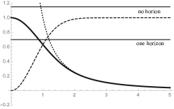
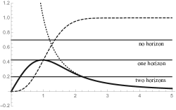
Figure 3: Profiles of $h_{0}(x)$ (left) and $h_{1}(x)$ (right). The horizontal lines denote the values of $(\sqrt{2\theta})^{2}/8M\ell^{2}$. $h_{1}(x)$ is chosen as a typical example for $n\geq 1$. For comparison, $x^{-2}$ and $\gamma(n/2+1,x^{2})/\Gamma(n/2+1)$ are plotted in the dashed and the dotted curves, respectively.

If the dimensionless constant $(\sqrt{2\theta})^{2}/8M\ell^{2}$ is smaller than the maximum value of $h_{n}(x)$, there exist a horizon. For $n=0$, since $0\leq h_{0}(x)<1$, a horizon is formed when

$$0<\frac{(\sqrt{2\theta})^{2}}{8M\ell^{2}}<1.$$ (3.37)

If $8M\ell^{2}/(\sqrt{2\theta})^{2}=1$, there is a “black hole” at $r=0$ whose radius is zero. So this condition can be read as there must be enough mass within a radius for a horizon to be formed compared with the noncommutative parameter $\theta$ which determines how much the mass is diffused and is leaked out of the radius . This is a reasonable claim.

For $n\geq 1$, the horizon formation condition is given by

$$0<h_{n}^{*}\leq 1\quad\Leftrightarrow\quad M\geq\frac{(\sqrt{2\theta})^{2}}{8h_{n}^{*}\ell^{2}}=M_{*},$$ (3.39)

where $h_{n}^{*}$ is the maximum value of $h_{n}(x)$. When $M>M_{*}$, there are two horizons. The existence of two horizons is one of the peculiar features for $n\geq 1$. If $M=M_{*}$, it is extremal and there exist the black hole with one horizon, whose Hawking temperature is zero. We can expect that, starting from a state with $M>M_{*}$, the mass $M$ will decrease by the Hawking radiation to the extremal. The existence of the extremal state means that there will be a remnant after the Hawking radiation even for such a uncharged, non-rotating black hole. One more difference between $n=0$ and $n\geq 1$ is about the energy conditions they satisfy. As mentioned in [6] where the four-dimensional case with $n=0$ is considered, the strong energy condition is violated for the energy-momentum tensor given in [6], but the weak energy condition is satisfied. In the three-dimensional cases, the weak energy condition is satisfied in the whole spacetime only for $n=0$. For $n\geq 1$, the weak energy condition ($\rho\geq 0$ and $\rho+p_{i}\geq 0$) is translated to

$$\rho_{n}\geq 0,\quad\rho_{n}+p_{nr}\geq 0,\quad\rho_{n}+p_{n\phi}\geq 0.$$ (3.40)

We can explicitly check that the first and second condition are always satisfied. The third one is rewritten as

$$\rho_{n}+p_{\phi}\propto r^{n}\left(r^{2}-n\theta\right)e^{-\frac{r^{2}}{2\theta}}\geq 0.$$ (3.41)

Therefore $\rho_{n}+p_{n\phi}$ is not necessarily positive in the whole space. We leave the detail analysis and physical meaning of it for a sequent paper.

Although the existence of the black holes with two horizons for $n\geq 1$ naively appears that the noncommutativity works as a repulsive force in the vicinity of the centers of the black holes just like the RN case, it is not completely true. In fact, in the three-dimensional case we have seen above, there is no black hole with two horizons for $n=0$. This was pointed out in [23] and the authors analyzed the difference of the behaviors for $n=0$ and $n=1$.

Actually, the regularity in the whole space is realized because of the fuzziness of the source. This can be understood by the Ricci scalar at $r=0$. Using (3.21), we can calculate the Ricci scalar at the center of the spacetime as

$$R|_{r=0} = \begin{cases}\displaystyle\frac{6}{\ell^{2}}\left(-1+\frac{8M\ell^{2}}{(\sqrt{2\theta})^{2}}\right)&(n=0),\vspace{0.3cm}\\ \displaystyle-\frac{6}{\ell^{2}}&(n\geq 1).\end{cases}$$ (3.42)

For $n\geq 1$, the Ricci scalar becomes a negative constant at $r=0$, which is consistent with the fact the mass function with $n\geq 1$ is zero at $r=0$ and the negative cosmological constant $\Lambda=-1/\ell^{2}$ is dominant there. For $n=0$, there are three cases depending on the value of $8M\ell^{2}/(\sqrt{2\theta})^{2}$. To be more concrete, we find

$$R|_{r=0}=\frac{8M\ell^{2}}{(\sqrt{2\theta})^{2}}\begin{cases}>1&:\mbox{de Sitter},\\ =1&:\mbox{flat},\\ <1&:\mbox{anti de Sitter}.\end{cases}$$ (3.43)

As shown in (3.37), when a horizon is formed, $8M\ell^{2}/(\sqrt{2\theta})^{2}$ is always larger than 1. There is a de Sitter core in the center of the spacetime, which is similar to the four-dimensional case [6].

It is true that in four dimensions, there exist a black hole with two horizons even for $n=0$ as long as the mass is large enough. To understand the difference between the three- and the four-dimensional cases, we have to compare the characteristic functions for their horizon formation conditions. In the four-dimensional case, the condition is shown in (2.19). The essential part of the characteristic function is given by

$$h_{4d}(x)\sim\frac{1}{x}\gamma\left(\frac{n+3}{2},x^{2}\right),$$ (3.44)

for an arbitrary $n$, where $\sim$ denotes that we are extracting the relevant term. On the contrary, in the three-dimensional case, the counterpart is given by

$$h_{n}(x)\sim\frac{1}{x^{2}}\gamma\left(\frac{n+1}{2},x^{2}\right).$$ (3.45)

The essential difference is the power of $x$ in front of the lower incomplete gamma function that controls the behavior around $x=0$. It is clearly originated from the difference of dimensions and intrinsic structures due to them that appears in $g_{tt}=g_{rr}^{-1}$ rather than noncommutativity.

To see it more clearly, let us consider a simple toy model in three dimensions whose density is given by

$$\rho(r)=\begin{cases}\displaystyle\frac{3M}{2\pi R^{3}}r&(0\leq r\leq R),\vspace{0.3cm}\\ 0&(R<r),\end{cases}$$ (3.46)

where $R$ is a characteristic scale of length of the system. The profile of $\rho(r)$ is shown in Fig.4. The mass function for this density is

$$m(r)=2\pi\int_{0}^{r}dr^{\prime}r^{\prime}\rho(r^{\prime})=\begin{cases}\displaystyle M\left(\frac{r}{R}\right)^{3}&(0\leq r\leq R),\\ M&(R<r).\end{cases}$$ (3.47)

Note that this model is not realistic in the sense that there is a gap the density and the mass function at $r=R$, however, it is not crucial in the following argument on the existence of a horizon. Actually, though we can consider a density that is smooth at $r=R$ and has an almost same profile as this toy model, it would not give an essential improvement to understand the horizon formation condition.

Then repeating the same argument for the three-dimensional black hole with the generalized Gaussian source, we find that the horizon formation condition is given by

$$\frac{R^{2}}{8M\ell^{2}}\leq h_{toy}(y)\equiv\begin{cases}\displaystyle y&(0<y\leq 1),\vspace{0.3cm}\\ \displaystyle\frac{1}{y^{2}}&(1\leq y),\end{cases}$$

where $y$ is a dimensionless parameter defined by $y=r_{h}/R$. The characteristic function for the horizon formation condition is shown in Fig.4.

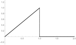
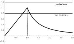
Figure 4: Plots of the toy density (left) and the characteristic function $h_{toy}(y)$ (right).

The extreme case corresponds to $y=1\ \Leftrightarrow\ R=\sqrt{8M\ell^{2}}$. For $R<\sqrt{8M\ell^{2}}$, there are two horizons. This existence of two horizons, in particular the existence of the inner horizon in this case, is a resultant of the void of the mass distribution around the center. This implies that there might exist a black hole with two horizons as long as there is a void around the center and enough mass is condensed in a given region, even if the spacetime noncommutativity does not work directly.

4 Regular black hole and fuzzy disc

4.1 Fuzzy disc as a source of a three-dimensional black hole

The analysis so far can be applied to other type of sources inspired from noncommutative geometry in three dimensions. In [29], we considered the fuzzy disc, which is a disc-shaped region in a two-dimensional Moyal plane [30, 31, 32]. A Moyal plane is a flat space defined by noncommutative coordinates satisfying the commutation relation $[x,y]=i\theta$. The algebra of functions on this noncommutative plane is an operator algebra $\hat{\cal A}$ generated by $\hat{x}$ and $\hat{y}$, acting on a Hilbert space ${\cal H}=l^{2}={\rm span}\{\left|\,{0}\,\right\rangle,\left|\,{1}\,\right\rangle,\cdots\}$. Here $\left|\,{n}\,\right\rangle$ is an eigenstate of “the number operator”

$$\hat{N}\left|\,{n}\,\right\rangle=n\left|\,{n}\,\right\rangle,\quad\hat{N}\equiv\hat{a}^{\dagger}\hat{a},$$ (4.1)

defined by the creation and the annihilation operators, $\hat{a}=(\hat{x}+i\hat{y})/\sqrt{2\theta},\ \hat{a}^{\dagger}=(\hat{x}-i\hat{y})\sqrt{2\theta}$, respectively.

The fuzzy disc is defined by using an operator algebra $\hat{\cal A}$ on a Moyal plane by restricting to $N\times N$ matrices in the number basis. It is obtained by the projection $\hat{\cal A}_{N}=\hat{P}_{N}\hat{\cal A}\hat{P}_{N}$ through the rank $N$ projection operator,

$$\hat{P}_{\scriptscriptstyle N}=\sum_{n=0}^{N-1}\hat{p}_{n}=\hat{p}_{0}+\cdots+\hat{p}_{\scriptscriptstyle N-1},$$ (4.2)

where

$$\hat{p}_{n}=\left|\,{n}\,\right\rangle\left\langle\,{n}\,\right|\quad(n=0,1,\cdots).$$ (4.3)

Instead of working with the operators, one can switch to the corresponding functions called symbols by means of the Weyl-Wigner correspondence. The symbol map based on this correspondence associates an operator $\hat{f}$ with a function $f$ as

$$f(z,\overline{z})=\left\langle\,{z}\,\right|\hat{f}\left|\,{z}\,\right\rangle,$$ (4.4)

where $z=re^{i\phi}$ and $\left|\,{z}\,\right\rangle$ is a coherent state defined by

$$\hat{a}\left|\,{z}\,\right\rangle=\frac{z}{\sqrt{2\theta}}\left|\,{z}\,\right\rangle.$$ (4.5)

Then, the corresponding function to the projection operator $\hat{p}_{n}$ is given by

$$p_{n}(r)=\left\langle\left.\,{z}\,\right|\,{n}\,\right\rangle\left\langle\left.\,{n}\,\right|\,{z}\,\right\rangle=e^{-\frac{r^{2}}{2\theta}}\frac{r^{2n}}{n!(2\theta)^{n}},$$ (4.6)

which is one of the realizations of the density distribution described by the generalized Gaussian function in the context of noncommutative geometry. Here we used

$$\left\langle\left.\,{z}\,\right|\,{n}\,\right\rangle=e^{-\frac{r^{2}}{4\theta}}\frac{\overline{z}^{n}}{\sqrt{n!(2\theta)^{n}}},\quad\left\langle\left.\,{n}\,\right|\,{z}\,\right\rangle=e^{-\frac{r^{2}}{4\theta}}\frac{z^{n}}{\sqrt{n!(2\theta)^{n}}}.$$ (4.7)

One can obtain the corresponding function for the fuzzy disc as well. Since the fuzzy disc is a sum of the $N$ projection operators from $n=0$ to $n=N-1$, the corresponding function for the fuzzy disc is given by

$$P_{\scriptscriptstyle N}(r)=\sum_{n=0}^{N-1}e^{-\frac{r^{2}}{2\theta}}\frac{r^{2n}}{n!(2\theta)^{n}}=\frac{\Gamma(N,\frac{r^{2}}{2\theta})}{\Gamma(N)}.$$ (4.8)

This function is roughly a radial step function that picks up a disc-shaped region around the origin $r=0$ with radius $R=\sqrt{2N\theta}$. On more details of how to find the corresponding function to an operator, one can find in [29].

We now use the fuzzy disc as a source for a noncommutative inspired black hole in three dimensions. As a density motivated by the fuzzy disc (4.8), we consider a spacetimes with a density distribution

$$\rho_{\scriptscriptstyle N}^{\scriptscriptstyle FD}(r)=\frac{M}{2\pi\theta N}P_{\scriptscriptstyle N}(r)=\frac{M}{2\pi\theta}\frac{\Gamma(N,\frac{r^{2}}{2\theta})}{\Gamma(N+1)}.$$ (4.9)

The density distributions (that is, the shapes of the fuzzy discs) and the mass functions $m_{\scriptstyle N}^{\scriptscriptstyle FD}(r)$ for $N=1,2,3$ are shown in Fig.5 and Fig.6, respectively. They are normalized as

$$m_{\scriptscriptstyle N}^{\scriptscriptstyle FD}(\infty)=2\pi\int_{0}^{\infty}dr^{\prime}r^{\prime}\rho_{N}(r)=M,$$ (4.10)

as before.

Since the radius of the fuzzy disc is almost $\sqrt{2N\theta}$, the radii are about $0.44,0.63,0.77$ for $N=1,2,3$ and $\theta=0.1$. The edge of the fuzzy disc becomes shaper as $N\to\infty$ with $N\theta=$ fixed. In Fig.7, we draw $N=100$ and $N=1000$ with $N\theta=1$ cases, respectively.

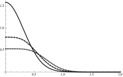
Figure 5: Plot of the density functions of the fuzzy disc type for $N=1$ (solid), $N=2$ (dashed) and $N=3$ (dotted). Here we set $M=1$ and $\theta=0.1$.

We can see that their radii are almost $\sqrt{2N\theta}\simeq 1.4$ in Fig.7.

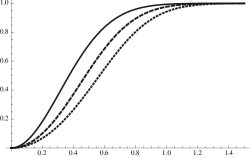
Figure 6: Plot of the mass functions corresponding to the fuzzy disc type source for $N=1$ (solid), $N=2$ (dashed) and $N=3$ (dotted). Here $M=1$ and $\theta=0.1$.

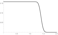
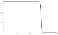
Figure 7: Plot of the density function for $N=100$ (left) and $N=1000$ (right) with $N\theta=1$. Their radii are $\simeq\sqrt{2N\theta}$.

Using the mass function

$$m_{\scriptscriptstyle N}^{\scriptscriptstyle FD}(r) = 2\pi\int_{0}^{r}dr^{\prime}r^{\prime}\rho_{N}(r^{\prime})$$ (4.11)

$$= \frac{M}{\Gamma(N+1)}\left[\gamma\left(N+1,\frac{r^{2}}{2\theta}\right)+\frac{r^{2}}{2\theta}\Gamma\left(N,\frac{r^{2}}{2\theta}\right)\right],$$ (4.12)

we explicitly write the horizon formation condition for the fuzzy disc as

$$m_{\scriptscriptstyle N}^{\scriptscriptstyle FD}(r_{h})\geq\frac{r_{h}^{2}}{8M\ell^{2}}.$$ (4.13)

Introducing $x=r_{h}/\sqrt{2\theta}$, this condition is rewritten as

$$h_{\scriptscriptstyle N}^{\scriptscriptstyle FD}(x)=\frac{1}{x^{2}}\left[1-\frac{\Gamma(N+1,x^{2})}{\Gamma(N+1)}\right]+\frac{\Gamma(N,x^{2})}{\Gamma(N+1)}\geq\frac{(\sqrt{2\theta})^{2}}{8M\ell^{2}}.$$ (4.14)

The profiles of $h_{\scriptscriptstyle N}^{\scriptscriptstyle FD}(x)$ for $N=1,2,3$ are shown in Fig.8.

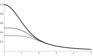
Figure 8: Plot of $h_{\scriptscriptstyle N}^{\scriptscriptstyle FD}(x)$ for $N=1$ (solid), $N=2$ (dashed) and $N=3$ (dotted).

Here $N$ denotes how many annuli are summed. The fuzzy disc with $N=1$ is constituted of $\left|\,{0}\,\right\rangle\left\langle\,{0}\,\right|$ only, and the fuzzy disc with $N=2$ is the sum of two annuli that corresponds to $\left|\,{0}\,\right\rangle\left\langle\,{0}\,\right|+\left|\,{1}\,\right\rangle\left\langle\,{1}\,\right|$, …, and so on.

If we choose an appropriate $(\sqrt{2\theta})^{2}/(8M\ell^{2})$, there can exist a black hole. For any $N$, as the characteristic function $h_{\scriptscriptstyle N}^{\scriptscriptstyle FD}(x)$ is monotonically decreasing, we find

$$\begin{cases}M\geq\displaystyle\frac{(\sqrt{2\theta})^{2}}{8h_{\scriptscriptstyle N}^{*}\ell^{2}}&:\mbox{one horizon},\vspace{0.5cm}\\ M<\displaystyle\frac{(\sqrt{2\theta})^{2}}{8h_{\scriptscriptstyle N}^{*}\ell^{2}}&:\mbox{no horizon},\end{cases}$$ (4.15)

where $h_{\scriptscriptstyle N}^{*}$ is the maximum of $h_{\scriptscriptstyle N}^{\scriptscriptstyle FD}(x)$.

The Ricci scalar of this spacetime is positive at $r=0$ for any $N$, which means that there is a de Sitter core there. This is same as the three-dimensional black hole with $\rho_{0}(r)\propto e^{-r^{2}/(2\theta)}$ as its source. Since the fuzzy disc source does not have a void in its center, its shape is similar to that described by $\rho_{0}(r)$. So this is reasonable.

4.2 Extension to a four-dimensional black hole

It is interesting to extend this fuzzy disc source to a four-dimensional spacetime. This extension corresponds to the source that is a sum of the thick matter layers considered in [9] with giving certain weights to the layers. For a three-dimensional case with the fuzzy disc as its source, two horizons can not be formed as we expected from the fact that there is no void around the centers. However, in four dimensions, the situation will change. In four dimensions, we consider the following density motivated by the fuzzy “disc”,

$$\rho_{\scriptscriptstyle N}^{\scriptscriptstyle 4dFD}(r)=\frac{3M}{4\pi(\sqrt{2\theta})^{3}\Gamma(N+\frac{3}{2})}\Gamma\left(N,\frac{r^{2}}{2\theta}\right),$$ (4.16)

and the mass function counterpart is given by

$$m_{\scriptscriptstyle N}^{\scriptscriptstyle 4dFD}(r)=\frac{M}{3\Gamma\left(N+\frac{3}{2}\right)}\left[\gamma\left(N+\frac{3}{2},\frac{r^{2}}{2\theta}\right)+\frac{r^{3}}{(\sqrt{2\theta})^{3}}\Gamma\left(N,\frac{r^{2}}{2\theta}\right)\right].$$ (4.17)

The horizon formation condition is determined by

$$h_{\scriptscriptstyle N}^{\scriptscriptstyle 4dFD}(x)=\frac{2}{3\Gamma(N+\frac{3}{2})}\left[\frac{1}{x}\gamma\left(N+\frac{3}{2},x^{2}\right)+x^{2}\Gamma(N,x^{2})\right],$$ (4.18)

where $x=r_{h}/\sqrt{2\theta}$ as before.

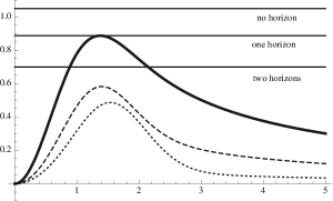
Figure 9: Plot of $h_{\scriptscriptstyle N}^{\scriptscriptstyle 4dFD}(x)$ for $N=1$ (solid), $N=2$ (dashed) and $N=3$ (dotted). The horizontal lines denote the values of $(\sqrt{2\theta})^{2}/8M\ell^{2}$. Though we draw the horizon formation condition only for $N=1$, the qualitative behavior does not change for an arbitrary $N$. In four dimensions, there is a black hole that can have two horizons if it holds an appropriate condition.

The behavior of $h_{\scriptscriptstyle N}^{\scriptscriptstyle 4dFD}(x)$ is shown in Fig.9. As we expected, $h_{\scriptscriptstyle N}^{\scriptscriptstyle 4dFD}(x)$ has only one extremum at finite $x$. $h_{\scriptscriptstyle N}^{\scriptscriptstyle 4dFD}(x)$ asymptotically approaches to zero when $x\to\infty$ and it becomes zero at $x=0$. We find that there is a black hole that can have two horizons as long as there is enough mass $M$ within a given volume. This is because the power of divergence of the characteristic function around $x=0$ is weakened from $x^{-2}$ in three dimensions to $x^{-1}$ in four dimensions.

We can conclude that there are three cases, that is, two horizons, one horizon (the extremal) and no horizon cases, respectively. For a black hole with two horizons, there would be a remnant after radiation from the black holes. It is true that the behaviors of the source terms depend on noncommutativity which is denoted by $\theta$, but we may have to say that the possibility of remnant is originated from the difference of dimensions and intrinsic structures of the spacetimes rather than noncommutativity.

5 Conclusion and discussion

In this paper, we considered the black holes in three and four-dimensional spacetimes. These black holes have the fuzzy sources inspired by noncommutative geometry. Noncommutativity between space coordinates is translated to the Gaussian profiles of matter distributions represented by the noncommutative parameter $\theta$.

As investigated by many authors, there can be a black hole with two horizons for such a source when enough mass is included within a given radius. In order to judge whether a horizon is formed or not, we introduced the mass functions. Introduction of them makes it possible to regard those black holes as Schwarzschild black holes with effective masses.

As an example, we first showed that how the mass function effectively works to investigate the horizon formation condition in the four-dimensional case with the density distribution represented by the generalized Gaussian function argued in [6, 9]. Next we applied this manner to the three-dimensional spacetime with the source described by the generalized Gaussian function. In the case of the three-dimensional spacetimes, the horizon formation condition depends on whether the mass function evaluated at a given radius is larger than the mass of the BTZ black hole. We analyzed the behaviors of the characteristic function for the horizon formation condition in detail and found how the difference between the three- and the four-dimensional spacetimes affects the horizon formation condition. The essential point of the horizon formation is the existence of a void around the center of the spacetime, which is closely relates to the spacetime’s dimension rather than noncommutativity that is expected to work as a repulsive force as a quantum effect. We saw this by giving the toy model that is apart from noncommutative geometry inspired models.

Since our point of view by means of mass function and characteristic function is graphical and intuitively understandable, we can easily apply it to any sources. In fact, we also considered the black hole with the source whose density distribution is motivated by the fuzzy disc. For such a fuzzy disc source with an arbitrary radius, a black hole can be formed as long as enough mass is included inside a given circle. This behavior is similar to the three-dimensional black hole with the density distribution $\rho\propto e^{-r^{2}/(2\theta)}$. This is interpreted as both distributions do not have a void at the centers of the spacetimes, but have de Sitter cores. The only difference between them is the length of the plateaus from the origin. We also considered the sources that have the same profile as the fuzzy disc in four dimensions. Since the fuzzy “disc” is an three-dimensional object, it is just a toy model to check how the difference of dimensions works on the horizon formation condition. In four dimensions, there can exist a black hole with two horizons for the source whose density distribution is motivated by the fuzzy disc.

As for a void, we want to state that it might be interesting to consider a source whose density distribution has the same profile as the fuzzy annulus we found in [29, 33]. The density distribution of the fuzzy annulus can be written by the linear combination of arbitrary number of the generalized Gaussian functions. According the argument so far, we expect that there could exist a black hole with two horizons even in three dimensions. Furthermore, there could be a black hole with more than two horizons because it is possible to put any gap between annuli. It is worth while analyzing the interior structure of such a spacetime relating to the Hawking radiation as a probe [34], which is left for a sequent paper. Also, the detail analysis on causal structure, geodesic motion of a particle, thermodynamics and so on would also be interesting.

References

- [1] P. Aschieri, M. Dimitrijevic, F. Meyer and J. Wess, Noncommutative geometry and gravity, Class. Quant. Grav. 23 (2006) 1883–1912 [hep-th/0510059].
- [2] P. Aschieri et. al., A gravity theory on noncommutative spaces, Class. Quant. Grav. 22 (2005) 3511–3532 [hep-th/0504183].
- [3] P. Aschieri and L. Castellani, Noncommutative Gravity Solutions, J. Geom. Phys. 60 (2010) 375–393 [0906.2774].
- [4] T. Asakawa and S. Kobayashi, Noncommutative Solitons of Gravity, Class. Quant. Grav. 27 (2010) 105014 [0911.2136].
- [5] S. Kobayashi and T. Asakawa, Emergence of Spacetimes and Noncommutativity, in Proceedings, 19th Workshop on General Relativity and Gravitation in Japan (JGRG19), Tokyo, Japan, 2009.
- [6] P. Nicolini, A. Smailagic and E. Spallucci, Noncommutative geometry inspired Schwarzschild black hole, Phys. Lett. B632 (2006) 547–551 [gr-qc/0510112].
- [7] S. Ansoldi, P. Nicolini, A. Smailagic and E. Spallucci, Noncommutative geometry inspired charged black holes, Phys. Lett. B645 (2007) 261–266 [gr-qc/0612035].
- [8] P. Nicolini and E. Spallucci, Noncommutative geometry inspired wormholes and dirty black holes, Class. Quant. Grav. 27 (2010) 015010 [0902.4654].
- [9] P. Nicolini, A. Orlandi and E. Spallucci, The final stage of gravitationally collapsed thick matter layers, Adv. High Energy Phys. 2013 (2013) 812084 [1110.5332].
- [10] E. Spallucci, A. Smailagic and P. Nicolini, Pair creation by higher dimensional, regular, charged, micro black holes, Phys. Lett. B670 (2009) 449–454 [0801.3519].
- [11] A. Smailagic and E. Spallucci, ’Kerrr’ black hole: the Lord of the String, Phys. Lett. B688 (2010) 82–87 [1003.3918].
- [12] L. Modesto and P. Nicolini, Charged rotating noncommutative black holes, Phys. Rev. D82 (2010) 104035 [1005.5605].
- [13] P. Nicolini, Noncommutative Black Holes, The Final Appeal To Quantum Gravity: A Review, Int. J. Mod. Phys. A24 (2009) 1229–1308 [0807.1939].
- [14] J. R. Mureika and P. Nicolini, Aspects of noncommutative (1+1)-dimensional black holes, Phys. Rev. D84 (2011) 044020 [1104.4120].
- [15] A. Larranaga, A. Cardenas-Avendano and D. A. Torres, On a general class of regular rotating black holes based on a smeared mass distribution, Phys. Lett. B743 (2015) 492–502 [1410.0049]. [Erratum: Phys. Lett.B747,564(2015)].
- [16] I. Dymnikova, Vacuum nonsingular black hole, Gen. Rel. Grav. 24 (1992) 235–242.
- [17] I. Dymnikova, Spherically symmetric space-time with the regular de Sitter center, Int. J. Mod. Phys. D12 (2003) 1015–1034 [gr-qc/0304110].
- [18] I. Dymnikova and E. Galaktionov, Stability of a vacuum nonsingular black hole, Class. Quant. Grav. 22 (2005) 2331–2358 [gr-qc/0409049].
- [19] F. Rahaman, P. K. F. Kuhfittig, B. C. Bhui, M. Rahaman, S. Ray and U. F. Mondal, BTZ black holes inspired by noncommutative geometry, Phys. Rev. D87 (2013), no. 8 084014 [1301.4217].
- [20] J. M. Tejeiro and A. Larranaga, Noncommutative Geometry Inspired Rotating Black Hole in Three Dimensions, Pramana 78 (2012) 155–164 [1004.1120].
- [21] A. Larranaga and J. M. Tejeiro, Three Dimensional Charged Black Hole Inspired by Noncommutative Geometry, Abraham Zelmanov J. 4 (2011) 28–35 [1004.1608].
- [22] F. Rahaman, P. Bhar, R. Sharma and R. K. Tiwari, Noncommutative geometry inspired -dimensional charged black hole solution in an anti-de Sitter background spacetime, Eur. Phys. J. C75 (2015), no. 3 107 [1409.0552].
- [23] Y. S. Myung and M. Yoon, Regular black hole in three dimensions, Eur. Phys. J. C62 (2009) 405–411 [0810.0078].
- [24] J. Liang, Y.-C. Liu and Q. Zhu, Thermodynamics of noncommutative geometry inspired black holes based on Maxwell-Boltzmann smeared mass distribution, Chin. Phys. C38 (2014) 025101.
- [25] E. Poisson, A Relativist’s Toolkit: The Mathematics of Black-Hole Mechanics. Cambridge University Press, 2007.
- [26] E. Spallucci, A. Smailagic and P. Nicolini, Non-commutative geometry inspired higher-dimensional charged black holes, Phys. Lett. B670 (2009) 449–454 [0801.3519].
- [27] M.-I. Park, Smeared hair and black holes in three-dimensional de Sitter spacetime, Phys. Rev. D80 (2009) 084026 [0811.2685].
- [28] R. Yamazaki and D. Ida, Black holes in three-dimensional Einstein-Born-Infeld dilaton theory, Phys. Rev. D64 (2001) 024009 [gr-qc/0105092].
- [29] S. Kobayashi and T. Asakawa, Angles in Fuzzy Disc and Angular Noncommutative Solitons, JHEP 04 (2013) 145 [1206.6602].
- [30] F. Lizzi, P. Vitale and A. Zampini, The fuzzy disc, JHEP 08 (2003) 057 [hep-th/0306247].
- [31] F. Lizzi, P. Vitale and A. Zampini, From the fuzzy disc to edge currents in Chern-Simons theory, Mod. Phys. Lett. A18 (2003) 2381–2388 [hep-th/0309128].
- [32] F. Lizzi, P. Vitale and A. Zampini, The fuzzy disc: A review, J. Phys. Conf. Ser. 53 (2006) 830–842.
- [33] S. Kobayashi and T. Asakawa, Fuzzy Objects and Noncommutative Solitons, in Proceedings, 13th Marcel Grossmann Meeting on Recent Developments in Theoretical and Experimental General Relativity, Astrophysics, and Relativistic Field Theories (MG13), Stockholm, Sweden, pp. 2522–2524, 2015.
- [34] Y. Deng and G. Cleaver, Hawking Radiation from Regular Black Hole as a Possible Probe for Black Hole Interior Structure, 1602.06035.