Trust-Aware Network Utility Optimization in Multihop Wireless Networks with Delay Constraints

Abstract

Many resource allocation problems can be formulated as a constrained maximization of a utility function. Network Utility Maximization (NUM) applies optimization techniques to achieve decomposition by duality or the primal-dual method. Several important problems, for example joint source rate control, routing, and scheduling design, can be optimized by using this framework. In this work, we introduce an important network security concept, “trust”, into the NUM formulation and we integrate nodes’ trust values in the optimization framework. These trust values are based on the interaction history between network entities and community based monitoring. Our objective is to avoid routing packets though paths with large percentage of malicious nodes. We also add end-to-end delay constraints for each of the traffic flows. The delay constraints are introduced to capture the quality of service (QoS) requirements imposed to each traffic flow.

I Introduction

The problem of resource allocation in wireless networks has been a growing area of research over the past decade. Recent advances in the area of network utility maximization (NUM) driven cross-layer design[1],[2],[3] have led to efforts on top-down development of next generation wireless network architectures. By linking decomposition of the NUM problem to different layers of the network stack, we are able to design protocols, based on the optimal NUM derived algorithms, which provide much better performance gain over the current network protocols.

Traditionally, network protocols are strictly layered. Source rate control, routing and scheduling (e.g. back-pressure scheduling[4]) are implemented independently at different layers. In order to achieve high performance and efficient resource utilization, these protocols should be jointly designed while the layered structure is preserved. However, the nature of wireless multihop networks imposes new challenges to this cross-layer design, since the wireless channel is a shared medium where the transmissions of users interfere with each other. The channel capacity is “elastic” (time-varying) and the contention over such shared and limited network resources provides a fundamental constraint for resource allocation. All these challenges cause interdependencies across users and network layers. In spite of these difficulties, there have been significant developments in optimization-based approaches that result in loosely coupled cross-layer solutions[5].

In recent years, network security has become increasingly important in the context of wireless multihop networks. Different types of network attacks can be released and affect significantly their performance. In our work, we consider that the adversary is capable of releasing some form of denial of service (DoS) attack. Hence, without proper security consideration, the network operation is possible to be disrupted. To capture the notion of security, we use “trust weights”[6] in the network utility optimization process. These weights indicate whether a network entity (node) is malicious or not, based on its interactions with the other network entities. Thus, by using them, we enhance the correct operation of the network and its resilience to attacks. The trust weights are developed by our network community based on monitoring and are disseminated via efficient methods so that they are timely available to all nodes that need them [7].

End-to-end delay is a critical quality of service (QoS) requirement for resource-constrained wireless networks. Network applications, served from different traffic flows in the wireless network, have different delay requirements. For example, video streaming applications are time-critical and have strict delay requirements. Hence, it is crucial to take into account these delay constraints, corresponding to different classes of traffic flows, to our trust-aware NUM problem.

In this paper, we incorporate the notion of security into the NUM problem, by using the trust values of the network nodes. Users get higher utility, when they relay packets though trusted paths. Hence, our proposed trust-aware NUM process ensures that untrusted paths (with malicious entities) will not receive high traffic rate. We also add end-to-end delay constraints in the NUM problem based on [8]. These delay constraints indicate the QoS requirements of the different traffic flows. The notion of link capacity margin [8] is used to control the end-to-end delay. Finally, we propose a distributed cross-layer optimization algorithm for the trust-aware NUM problem with delay constraints. The distributed algorithm is based on the dual decomposition into source rate control, average end-to-end delay control and scheduling subproblems.

The rest of this paper is organized as follows. Section II reviews the related work in the literature on network utility maximization (NUM) problem formulation and its security considerations. Section III introduces the system model that we consider in this paper, including the network model, the adversary model, the trust values estimation, and the interference model. Section IV outlines the optimization constraints, which include link capacity, average end-to-end delay, and scheduling constraints, as well as the primal optimization problem. The dual function and its decomposition into different subproblems is studied in Section V. Section V-D discusses the distributed algorithm for solving the network utility maximization (NUM) problem. The simulation results for our proposed trust-aware NUM problem with delay constraints are shown in Section VI. Section VII concludes this paper and discusses future work.

II Related Work

Network utility maximization (NUM) problems have been investigated widely during recent years. Most of works [1], [2], [3], [5] focus on using NUM for cross-layer optimization. Chiang et. al [1] introduced a methodology for optimizing functional modules of the network, such as congestion control, routing and scheduling, through optimization decomposition. Chen et. al [2] proposed a subgradient algorithm for cross-layer optimization and its extension to time-varying channels and adaptive multi-rate devices. The proposed solution in most of these works depends on the decomposition of the dual function to different subproblems. Decomposition methods for NUM problem are proposed in [9].

Several works have introduced delay considerations for the traffic flows into the NUM problem formulation. Trichakis et. al [10] proposed a dynamic NUM formulation with delivery contracts for the different traffic flows. Delivery contracts ensure that some quantity of a traffic flow will be delivered during a time interval. One other concept for delay, used for the NUM problem, is the link capacity margins, which we use in our work. These margins were introduced in [8] and [11] to control the average end-end delay. Link margins represent the estimated delay of the link, because higher link margin indicates lower link congestion and thus less delay.

As far as we are concerned, there are not a lot of works that relate security with the NUM problem [12], [13]. Tague et. al [13] proposed a jamming-aware throughput maximization approach. The authors estimate the effect of jamming on packet delivery ratio. Then, they use these jamming estimates in the NUM problem to allocate data traffic appropriately in order to achieve throughput maximization. They adopt an objective function, based on portfolio selection theory to maximize throughput for the different source nodes.

To the best of our knowledge, our work is the first to study trust-aware network utility maximization problems. Trust values affect the outcome of the NUM process and make it resilient to malicious nodes’ behavior.

III System Model

III-A Network Model

We consider a multihop wireless network that can be defined by a graph $G(\mathcal{N},\mathcal{L})$. The vertex set $\mathcal{N}$ represents the wireless network nodes. The edge set $\mathcal{L}$ represents the wireless links. An ordered pair of nodes $(i,j)$ belongs to the edge set $\mathcal{L}$ if and only if node $j$ can receive data packets directly from node $i$. For simplicity, we also use the symbol $\ell$ to denote a wireless link. We assume that all node-to-node communication is unicast, i.e. each packet transmitted by a node $i\in{\mathcal{N}}$ is intended for a unique $j\in{\mathcal{N}}$ with $(i,j)\in\mathcal{L}$. Each of the wireless links has a maximum capacity denoted by $c_{i,j}$. The interference constraints among transmission links will be described in a later subsection.

There is a set $\mathcal{F}$ of network traffic flows that share the wireless network resources and each flow $f\in{\mathcal{F}}$ is associated with a source node $s$. Each source node $s$ in a subset $\mathcal{S}\subseteq{\mathcal{N}}$ generates data packets for a single destination node $d_{s}\in\mathcal{N}$. We assume that each source node $s$ constructs multiple routing paths with multiple hops to $d_{s}$ in order to distribute the traffic demand and satisfy the flow related QoS requirements. We denote as $\mathcal{P}_{s}=\{p_{s1},\ldots,p_{sP_{s}}\}$ the collection of the alternative paths $P_{s}$ that can be used to route packets from $s$ to $d_{s}$. Each path $p_{sk}\in{\mathcal{P}_{s}}$ is specified by a subset of wireless links and is assumed to be loop-free. An example of two different paths $p_{s1}$ and $p_{s2}$ from $s$ to $d_{s}$ is shown in Figure 1, where

$$p_{s1} =\{(s,1),(1,2),(2,3),(3,d_{s})\}$$

$$p_{s2} =\{(s,1),(1,4),(4,5),(5,d_{s})\}$$

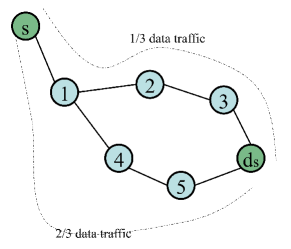
Figure 1: Network with two alternative paths for traffic flow from $s$ to $d$.

Let $\mathbf{x_{s}}$ denote the $P_{s}\times{1}$ traffic rate vector with which data packets are sent from $s$ to $d_{s}$ over multiple paths $p_{sk}\in{\mathcal{P}_{s}}$, and multiple hops. Each component of the vector $x_{sk}$ denotes the proportion of traffic rate allocated to the corresponding path $p_{sk}$, which routes data packets from source node $s$ to destination $d_{s}$. The total data rate of the source $s$ is given by the summation of $x_{sk}$ over $k=1,\ldots,{P_{s}}$.

We assume that the traffic rate vector $\mathbf{x_{s}}$ of each flow is constrained to a non-negative orthant. The traffic rate allocated to each traffic flow should also not exceed a maximum data rate $\mathcal{R}_{s}$. Therefore, each of the traffic rate vectors $\mathbf{x_{s}}$ should satisfy the following constraints

$$\mathbf{x_{s}}\geq\mathbf{0} \hskip 10.0pt,\forall{s\in\mathcal{S}}$$ (1)

$$\mathbf{1}^{T}\mathbf{x_{s}}\leq{\mathcal{R}_{s}} \hskip 10.0pt,\forall{s\in\mathcal{S}}$$ (2)

In Eq. (1) each component of the vector is nonnegative. These constraints define the convex set $\mathcal{X}_{s}$ of feasible traffic rate vectors $\mathbf{x_{s}}$ for source node $s$.

We denote by $\mathbf{R_{s}}=[(R_{s})_{k(i,j)}]_{(P_{s}\times|\mathcal{L}|)}$ the routing matrix that indicates the different paths from source node $s$ to destination $d_{s}$. Element $(R_{s})_{k(i,j)}$ of the routing matrix is defined as follows

$$(R_{s})_{k(i,j)}=\begin{cases}1,&\text{if $p_{sk}$ passes through link $(i,j)$}.\\ 0,&\text{otherwise}.\end{cases}$$ (3)

III-B Security Considerations: Adversary Model and Trust

In this paper, we study the network utility optimization problem with considerations of network security. All previous works on the network utility maximization (NUM) problems assume that nodes operate correctly. For example, intermediate nodes successfully forward all packets, and they follow the routing and scheduling protocols. However, nodes do not always function correctly in reality. They may be compromised by attackers, their communication may be blocked or interfered by attackers, or they may just be misconfigured. Wireless networks are especially vulnerable to attacks because of the inherent properties of the shared wireless medium. Therefore, we believe it is crucial to take the security aspect into consideration in the NUM problems. We are going to define the adversary model, which describes the capabilities of an adversarial node, and the notion of trust, which indicates whether a node can be considered as trustworthy based on its observed behavior.

Adversary Model: We assume that the adversarial node is not following the network protocol and attempts to disrupt communication by dropping or modifying data packets. In this work, we mainly consider that the adversary is capable of dropping data packets in a deterministic or probabilistic way. This type of attack leads to lack of availability of the network and constitutes a denial of service (DoS) attack. The DoS attack affects significantly some QoS requirements, such as end-to-end delay and packet delivery ratio. Thus, in order to support time-critical applications, the traffic allocation mechanisms should be resilient to these types of attacks. In general, the notion of trust can also address different types of attacks, such as the modification or fabrication of data messages. In this case, trust evaluation should incorporate authentication or inspection (filtering) mechanisms (e.g. Message Authentication Codes (MAC) or Deep Packet Inspection (DPI) [14]) at the receiver and intermediate nodes, in order to define the trustworthiness of a network node.

Trust Estimates: The concept of security, which we adopt to distinguish misbehaving nodes in this work is trust. Trust is a very critical concept not only in computer networks, but also in various other networks that involve intelligent decisions, such as social networks. All the connections and communications in these networks imply the existence of trust. Trust integrates with several components of network management, such as risk management, access control and authentication.

Trust management is to collect, analyze and present trust related evidence and to make assessments and decisions regarding trust relationships between entities in a network [15]. The collection of trust evidence and the decision of trust are beyond the scope of this paper. We assume that there are mechanisms to efficiently distribute trust evidence, such that duplicates of evidence documents are stored in places where they are most needed. Different approaches of trust evidence distribution could be found in [16] and [17] (use of network coding to efficiently distribute trust credentials among network entities). Once the trust evidence is in hand, nodes could evaluate the trustworthiness of other nodes. For instance, in wireless environments, the monitoring mechanisms can help detect the behaviors of neighboring nodes and thus infer their trust values[7]. We define the trust estimated value (or trustworthiness) of node $i$ as $\nu_{i}$.

There are various ways to represent trust values $\nu_{i}$ numerically. In different trust schemes, continuous or discrete numerical values are assigned to measure the level of trustworthiness for a network entity. For example, in [18] the entity’s opinion about the trustworthiness of a digital certificate is defined as a continuous value in $[0,1]$. Using the same logic for our definition of trust, we denote that it takes a continuous numerical value in $[0,1]$.

We define an update period of the trust estimates denoted by $T_{update}$. During the update period, represented by the time interval $[t-T_{update},t]$, the trust evaluation mechanism provides fresh estimates of the trust values for nodes $i\in\mathcal{S}$, based on the interaction between network entities. Each node evaluates trust estimates for its neighbor nodes and then the trust mechanism propagates the trust estimates throughout the network. Hence, at the time that we need to transmit data packets, we use the trust estimates derived at the latest update period.

In order to prevent significant variation in the trust estimate $\nu_{i}$ of node $i$ and to include memory of the trust evaluation, we suggest using an exponential weighted moving average (EWMA) [19] to update the trust estimate as a function of the previous estimate, as indicated in [13]. Hence, the trust value of node $i$ at time $t$ is given by

$$\nu_{i}(t)=(1-\alpha){\nu_{i}(t-T_{update})}+\alpha\nu_{i}^{new},$$ (4)

where $\alpha\in[0,1]$ is a constant weight indicating the relative preference between updated and historic samples of trust values and $\nu_{i}^{new}$ is the fresh estimate of trust value for node $i$, given from the trust evaluation mechanism.

Given the trust values for the intermediate nodes across a path $p_{sk}$, the source node $s$ evaluates the updated aggregate trust value for the path $p_{sk}\in\mathcal{P}_{s}$. The aggregate trust value of the path $p_{sk}$ is denoted by $t_{sk}$ and can be expressed as the product of the corresponding trust values along the path as follows

$$t_{sk}=\prod_{j:(i,j)\in{p_{sk}}}\nu_{j}$$ (5)

Source nodes evaluate the aggregate trust values for their alternative routing paths to destination $d_{s}$, in order to determine the optimal traffic allocation among the different paths.

One additional parameter that we should consider in the data traffic allocation process is path reliability [20]. In our work, path reliability is indicated by the corresponding aggregate trust value $t_{sk}$ over the path $p_{sk}$, which denotes the proportion of the allocated traffic flow that is actually received at destination node $d_{s}$. Hence, in order to maintain the reliability of the network the received traffic rate for each traffic flow should exceed a certain threshold. We denote this threshold for each source node $s$ as $\mathcal{R}^{thres}_{s}$, which is proportional to the maximum allowable rate $\mathcal{R}_{s}$. Thus, our allocated traffic rate for each source node should satisfy the reliability constraint expressed as

$$\sum_{p_{sk}\in\mathcal{P}_{s}}t_{sk}x_{sk}\geq{\mathcal{R}^{thres}_{s}},\hskip 10.0pt\forall{s\in\mathcal{S}}$$ (6)

The convex set $\mathcal{X}_{s}$ of feasible traffic rate vectors for source node $s$ should also satisfy the above reliability constraint.

III-C Interference model and capacity region

In this subsection, we describe the interference model and the feasible capacity region. In order to model interference among wireless links of our original wireless multihop network, we use the concept of the conflict graph introduced in [21]. The conflict graph captures the contention relations among the links. Each vertex in the conflict graph indicates a wireless link and each edge indicates the interference between the two corresponding links.

We can detect all the independent sets of vertices in the conflict graph. We denote an independent set of links by $e$. The independent set $e$ can be represented as a $\mathcal{|L|}\times 1$ capacity vector $r^{e}$. The element $r^{e}_{i,j}$ is expressed as

$$r^{e}_{i,j}=\begin{cases}c_{i,j},&,\text{if $(i,j)\in{e}$}.\\ 0&,\text{otherwise}.\end{cases}$$ (7)

The links that belong in an independent set do not interfere and are allowed to transmit simultaneously. The feasible capacity region $\Lambda$ [2] is defined as the convex hull of these capacity vectors and is expressed as

$$\Lambda=\Big{\{}r:r=\sum_{e}{\beta_{e}r^{e}},\beta_{e}\geq{0},\sum_{e}{\beta_{e}}=1\Big{\}}$$ (8)

Hence, the scheduling constraint indicates that the allocated capacity vector from the scheduling process, denoted by $\mathbf{\hat{c}}$, should satisfy $\mathbf{\hat{c}}\in\Lambda$.

IV Network Utility Maximization Formulation

In this section, we present the optimization framework for trust-aware network utility maximization (NUM), in the case that the network nodes have an updated estimate of trust values. We first develop a set of constraints imposed to our utility optimization problem. These constraints are related to capacity of wireless links, average end-to-end delay and scheduling. Then, we formulate the trust-aware utility optimization problem, which gives an optimal solution to the traffic flow allocation problem.

IV-A Optimization Constraints

Link Capacity constraint: To define capacity constraints we first introduce the link capacity margin optimization variables, which were initially introduced in [8] and [11], in order to capture the imposed delay constraints. We denote by $\sigma_{i,j}$ or simply $\sigma_{\ell}$, the link capacity margin of link $(i,j)\in\mathcal{L}$. Link capacity margin is defined as the difference between scheduled (allocated) capacity of a wireless link and the maximum allowable traffic flow passing though it. Link capacity margin is used to control link delay and therefore the average end-to-end delay.

We also need to take into account our trust estimates for the capacity constraints of each link $(i,j)\in{\mathcal{L}}$. Based on the capabilities of the malicious nodes, described in Section III-B, the initially allocated traffic rate $x_{sk}$ can be significantly reduced at malicious intermediate nodes because of dropping attacks. The decrease of the traffic rate is proportional to the aggregate trust value of the selected path. To be more specific, the decrease of the rate observed at an intermediate node is proportional to the aggregate trust value up to this intermediate node. Let $p_{sk}^{(i,j)}$ denote the sub-path of $p_{sk}$ from source node $s$ to the intermediate node $j$ through link $(i,j)\in p_{sk}$. Then the traffic rate forwarded by intermediate node $j\in\mathcal{N}$ is computed by $t_{sk}^{(i,j)}x_{sk}$, where $t_{sk}^{(i,j)}$ is evaluated as the product of trust estimates over the sub-path $p_{sk}^{(i,j)}$, given by Eq. (5).

Hence, the capacity constraint associated with each wireless link $(i,j)\in{\mathcal{L}}$ is formulated as follows

$$\sum_{s\in\mathcal{S}}\sum_{k:(i,j)\in{p_{sk}}}{t_{sk}^{(i,j)}x_{sk}}\leq{\hat{c}}_{i,j}-\sigma_{i,j},\hskip 8.0pt\forall{(i,j)\in{\mathcal{L}}},$$ (9)

where $\hat{c}_{i,j}$ is the capacity allocated to the wireless link $(i,j)\in{\mathcal{L}}$.

To define the different sub-paths’ aggregate trust values, we denote by $\mathcal{T}_{s}$ the $P_{s}\times{|\mathcal{L}|}$ aggregate trust incidence matrix for source $s$, with rows indexed by the alternative paths $p_{sk}$ and columns indexed by links $(i,j)$. If a link $(i,j)$ does not belong to any of the possible paths $p_{sk}$ for source $s$, then the corresponding entry of the incidence matrix is equal to $0$. The element $t(p_{sk},(i,j))$ or otherwise $t_{sk}^{(i,j)}$ for row $p_{sk}$ and column $(i,j)$ of $\mathcal{T}_{s}$ denotes the aggregate trust value of a possible sub-path $p_{sk}^{(i,j)}$ of path $p_{sk}$ and is given by

$$t(p_{sk},(i,j))=\begin{cases}\underset{j^{{}^{\prime}}:(i^{{}^{\prime}},j^{{}^{\prime}})\in{p_{sk}^{(i,j)}}}{\prod}\nu_{j^{{}^{\prime}}}&,\text{if $(i,j)\in{p_{sk}}$}\\ 0&,\text{otherwise}\end{cases}$$ (10)

Average end-to-end delay constraint: By using the link margin variables $\sigma_{i,j}$, we define as $\phi(\sigma_{i,j})$ the delay of link $(i,j)\in{\mathcal{L}}$. The function $\phi(\cdot)$ is typically a strictly convex, nonnegative valued, function of $\sigma$. The packet arrival process model determines the way that $\phi(\cdot)$ depends on $\sigma_{i,j}$. As described in [8] and [11], for Poisson process arrival, we have

$$\phi(\sigma_{i,j})=\phi_{i,j}=\frac{1}{\sigma_{i,j}}$$ (11)

We define by $\phi(\sigma)$ the vector that has components the delay of all links of the network.

Delay constraints indicate the QoS requirements imposed to a specific traffic flow. Traffic flows that serve time-critical applications should have strict delay constraints. The end-to-end delay is expressed by adding the link delays for each of the links over path $p_{sk}$ of source node $s$. We denote the upper bound average delay constraint for each of the multiple paths of the source node $s$ as $\mathcal{D}_{s}>0$. Hence, we have that the average end-to-end delay constraint for every source node $s$ is given by (using the routing matrix expressed in Eq. (3))

$$\mathbf{R_{s}}{\bf{\phi(\sigma)}}\leq\mathbf{1}\mathcal{D}_{s},\hskip 10.0pt\forall{s\in{\mathcal{S}}}$$ (12)

Scheduling constraint: The capacity $\hat{c}_{i,j}$ allocated to the wireless link $(i,j)$ should lie on the capacity region specified by $\Lambda$, which we describe in Sec. III-C. Hence, our scheduling constraint is expressed as

$$\mathbf{\hat{c}}\in\Lambda$$ (13)

IV-B Utility Optimization

To determine the optimal traffic rate allocation to the different paths $\mathcal{P}_{s}$, each source $s$ chooses a utility function $\mathcal{U}_{s}(\cdot)$ that evaluates the total data rate delivered to the destination $d_{s}$. Utility functions $\mathcal{U}_{s}(\cdot)$ are chosen to be strictly concave, continuous, monotonically increasing and twice differentiable.

Trust estimates for the different paths $p_{sk}$ of a source node (defined in Sec. III-B) should be incorporated to the selected utility function $\mathcal{U}_{s}(\cdot)$. Source nodes should obtain greater utility when they decide to allocate higher traffic rate through routing paths with higher aggregate trust value $t_{sk}$. Hence, the utility function for each source node $s\in\mathcal{S}$ can be selected as

$$\mathcal{U}_{s}(\mathbf{x}_{s})=\sum_{p_{sk}\in\mathcal{P}_{s}}\Big{(}t_{sk}\log{(x_{sk})}\Big{)}$$ (14)

The primal utility optimization problem formulation, based on the capacity, average end-to-end delay and scheduling constraints described in Eq. (9), (12) and (13), is given by

$$\underset{\mathbf{x},\mathbf{\sigma},\mathbf{\hat{c}}}{\text{max}} \sum_{s\in\mathcal{S}}\mathcal{U}_{s}(\mathbf{x}_{s})$$ (15a)

s. t. $$\sum_{s\in\mathcal{S}}\sum_{k:(i,j)\in{p_{sk}}}{t_{sk}^{(i,j)}x_{sk}}\leq{\hat{c}}_{i,j}-\sigma_{i,j},\forall{(i,j)}$$ (15f)

$$\mathbf{R_{s}}{\bf{\phi(\sigma)}}\leq\mathbf{1}\mathcal{D}_{s},\hskip 43.0pt\forall{s\in{\mathcal{S}}}$$

$$0\leq\mathbf{1}^{T}\mathbf{x_{s}}\leq{\mathcal{R}_{s}},\hskip 41.0pt\forall{s\in\mathcal{S}}$$

$$\sum_{p_{sk}\in\mathcal{P}_{s}}t_{sk}x_{sk}\geq{\mathcal{R}^{thres}_{s}},\hskip 10.0pt\forall{s\in\mathcal{S}}$$

$$\mathbf{\hat{c}}\in\Lambda$$

The trust-aware utility optimization problem is a strongly convex optimization problem, due to the strict concavity assumption of $U_{s}(\cdot)$ and the convexity of the capacity region. Therefore, there exists a unique optimal solution for the above primal problem, which we refer to as $(\mathbf{x^{*}},\mathbf{\sigma^{*}},\mathbf{\hat{c}^{*}})$.

V Dual Decomposition Algorithm

In this section, we solve the utility optimization problem described in Eq. (15a) by applying dual decomposition [9], [22]. The decomposition of the optimization problem provides distributed algorithms, which solve the underlying optimization problem. We note that strong duality holds for our optimization problem (duality gap is zero) and thus we can solve it through its dual function.

We define the Lagrange multipliers (dual variables) associated with the capacity and average end-to-end delay constraints. Let $\mathbf{\lambda}$ denote the $|\mathcal{L}|\times{1}$ vector of link prices (dual variables) $\lambda_{i,j}$ (otherwise denoted by $\lambda_{\ell}$) associated with the capacity constraints for each wireless link. Also, let $\mathbf{\mu}_{s}$ denote the $P_{s}\times{1}$ vector of dual variables $\mu_{sk}$ associated with the average end-to-end delay constraints imposed to every traffic flow $s\in\mathcal{S}$.

In order to introduce the dual problem, we define the partial Lagrangian $L(\mathbf{x},\sigma,\hat{\textbf{c}},\lambda,\mu)$ of the optimization problem by using the inequality constraints given from Eq. (15f) and (15f)

$$L(\mathbf{x},\sigma,\hat{\textbf{c}},\lambda,\mu)=\\ \sum_{s\in\mathcal{S}}\mathcal{U}_{s}(\mathbf{x}_{s})-\sum_{(i,j)\in\mathcal{L}}{\lambda_{i,j}}\Big{(}\sum_{s\in\mathcal{S}}\sum_{k:(i,j)\in{p_{sk}}}{\Big{(}t_{sk}^{(i,j)}x_{sk}\Big{)}}-{\hat{c}}_{i,j}+\sigma_{i,j}\Big{)}\\ -\sum_{s\in\mathcal{S}}{\mu_{s}^{T}\Big{(}\mathbf{R_{s}}{\bf{\phi(\sigma)}}-\mathbf{1}\mathcal{D}_{s}\Big{)}}\\ =\sum_{s\in{\mathcal{S}}}{\Big{(}\mathcal{U}_{s}(\mathbf{x}_{s})-\sum_{(i,j)\in\mathcal{L}}\lambda_{i,j}\sum_{k:(i,j)\in{p_{sk}}}{\Big{(}t_{sk}^{(i,j)}x_{sk}\Big{)}}}\Big{)}\\ -\sum_{(i,j)\in\mathcal{L}}\Big{(}\phi_{i,j}{\Big{(}\sum_{s\in\mathcal{S}}\sum_{k:(i,j)\in{p_{sk}}}\mu_{sk}[(R_{s})_{k(i,j)}]\Big{)}+\lambda_{i,j}\sigma_{i,j}\Big{)}}\\ +\lambda^{T}\hat{\mathbf{c}}+\sum_{s\in{\mathcal{S}}}{\mu_{s}^{T}\mathbf{1}\mathcal{D}_{s}}=\\ \sum_{s\in{\mathcal{S}}}{\Big{(}\mathcal{U}_{s}(\mathbf{x}_{s})-(\lambda^{s})^{T}\mathcal{T}_{s}^{T}\mathbf{x}_{s}\Big{)}}-\sum_{(i,j)\in\mathcal{L}}\Big{(}{\phi_{i,j}\mu^{(i,j)}+\lambda_{i,j}\sigma_{i,j}\Big{)}}\\ +\lambda^{T}\hat{\mathbf{c}}+\sum_{s\in{\mathcal{S}}}{\mu_{s}^{T}\mathbf{1}\mathcal{D}_{s}},$$ (16)

where $\lambda^{s}$ is a sub-vector of the $\lambda$ dual variable and is associated with the constraint in Eq. (15f). It defines the $|\mathcal{L}|\times{1}$ column link price vector related to the links that belong to any of the paths $p_{sk}\in{\mathcal{P}_{s}}$ of a particular source node $s$ and is given by

$$\lambda^{s}_{i,j}=\begin{cases}\lambda_{i,j}&,\text{if $(i,j)\in\underset{{p_{sk}\in\mathcal{P}_{s}}}{\cup}{p_{sk}}$}\\ 0&,\text{otherwise}\end{cases}$$ (17)

and $\mu^{(i,j)}=\sum_{s\in\mathcal{S}}\sum_{k:(i,j)\in{p_{sk}}}\mu_{sk}[(R_{s})_{k(i,j)}]$ denotes the combination of dual variables $\mu$, which are related to a specific link $(i,j)$ and is associated with the constraint (15f).

The dual objective function $h(\cdot)$ is then expressed as

$$h(\mathbf{\lambda},\mathbf{\mu}) =\sup_{\mathbf{x}\in\mathcal{X}}\Big{\{}\sum_{s\in{\mathcal{S}}}{\Big{(}\mathcal{U}_{s}(\mathbf{x}_{s})-(\lambda^{s})^{T}\mathcal{T}_{s}^{T}\mathbf{x}_{s}\Big{)}}\Big{\}}$$ (18d)

$$+\sup_{\sigma\geq\mathbf{0}}\Big{\{}-\sum_{(i,j)\in\mathcal{L}}\Big{(}{\phi_{i,j}\mu^{(i,j)}+\lambda_{i,j}\sigma_{i,j}\Big{)}}\Big{\}}$$

$$+\sup_{\hat{c}\in\Lambda}\Big{\{}\lambda^{T}\hat{\mathbf{c}}\Big{\}}$$

$$+\sum_{s\in{\mathcal{S}}}{\mu_{s}^{T}\mathbf{1}\mathcal{D}_{s}}$$

The dual optimization problem is defined by minimizing the dual objective function [23] over the dual vector variables $\lambda$ and $\mu$ as follows

$$\underset{\mathbf{\lambda}\geq\mathbf{0},\mathbf{\mu}\geq\mathbf{0}}{\text{min}} h(\mathbf{\lambda},\mathbf{\mu})$$ (19)

For given dual variables $\mathbf{\lambda}$ and $\mathbf{\mu}$, we can identify in the above equation of $h(\mathbf{\lambda},\mathbf{\mu})$ three decoupled maximization problems which we can solve separately. These three problems correspond to source rate control in Eq. (18d), average end-to-end delay control in Eq. (18d), and scheduling in Eq. (18d) respectively.

By solving these three independent optimization problems we can derive the optimal values for the primal optimization problem $\mathbf{x^{*}}(\mathbf{\lambda},\mathbf{\nu})$, $\mathbf{\sigma^{*}}(\mathbf{\lambda},\mathbf{\mu})$ and $\mathbf{\hat{c}^{*}}(\mathbf{\lambda},\mathbf{\mu})$ (described in Eq. (15a)). Given these values, we can then solve the dual problem by minimizing $h(\mathbf{\lambda},\mathbf{\mu})$ over $\mathbf{\lambda},\mathbf{\mu}\geq\mathbf{0}$. There is no duality gap between the primal and the dual, because the capacity region $\Lambda$ [2], [21] is a convex set.

In the following subsections, we describe the decomposition of the dual objective function that leads to the cross-layer optimization problem and we specify the optimal solutions by solving these independent subproblems.

V-A Source rate control

Based on the dual decomposition the traffic rate vector of source node $s$ is determined by the first maximization subproblem in Eq. (18d). $U_{s}(\cdot)$ is a strictly concave scalar function of the rate vector variable $x_{s}$. The maximization problem in (18d) is maximization of a concave function subject to the convex constraints (15f) and (15f). Thus, it has a unique solution. $U_{s}(\cdot)$ is continuously differentiable. Hence, the maximum will be given by the numerical solution of the equation

$$\nabla{\mathcal{U}_{s}}(x_{s}^{*})=\mathcal{T}_{s}\lambda^{s},\hskip 10.0pt\forall{s\in\mathcal{S}}$$ (20)

as long as the resulting solution for $x_{s}^{*}$ is in the interior of the constraint set defined by (15f) and (15f). Otherwise the solution will lie at the corners of the constrained set defined by (15f) and (15f).

It is important to note that each source node $s$ is able to adjust its data rate vector using its local observations on the link prices $\lambda_{i,j}$ across the links of its multiple routing paths and the aggregate trust values of the different paths and their respective sub-paths.

V-B Average End-to-End Delay Control

The second subproblem of the dual decomposition described in Eq. (18d) is related to average end-to-end delay control based on the optimal values for the link capacity margin $\sigma_{i,j}$. Eq. (18d) is a strictly convex, minimization problem, subject to the constraint that all sigma are nonnegative. Thus, it has a unique solution. Function $\phi(\cdot)$ is a continuously differentiable function. Hence, the optimal values of $\sigma_{i,j}^{*}$ are obtained by solving the equations numerically

$$\frac{d\mathcal{\phi}}{d\mathbf{\sigma}}(\sigma_{i,j}^{*})\mu^{(i,j)}=-\lambda_{i,j},\hskip 10.0pt\forall{(i,j)\in\mathcal{L}}$$ (21)

By Eq. (21), we observe that the updated dual variable related to the corresponding wireless link is needed. Thus, explicit/implicit exchange of dual variables between the different data sources is enabled.

V-C Scheduling policy

The third problem of the dual decomposition determines the scheduling policy. The optimal value for the allocated link capacity $\hat{c}_{i,j}^{*}$ is given by Eq. (18d)

$$\hat{c}_{i,j}^{*}=\underset{\hat{c}_{i,j}\in{\Lambda}}{\operatorname{argmax}}{\sum_{(i,j)\in\mathcal{L}}{\lambda_{i,j}\hat{c}_{i,j}}}$$ (22)

We need to find a scheduling policy so that the aggregate link weight $\sum_{(i,j)\in\mathcal{L}}{\lambda_{i,j}\hat{c}_{i,j}}$ could be maximized. The solution to this scheduling subproblem is based on the maximum weight scheduling policy introduced in [8]. This policy is described in Alg. 1.

Algorithm 1 Maximum-Weight Scheduling Policy [8]

1:  Start scheduling timer

2:  while Timer is ON do

3:     if $i$ has been scheduled by any of its neighboring nodes then

4:        Send messages to notify all nodes in its interference set and stop the process.

5:     else

6:        Each incident link $(i,j)$ is assigned a weight $\lambda_{i,j}\hat{c}_{i,j}$.

7:        Find a link with the maximum weight among all incident links.

8:        if link $(i,j)$ is found then

9:           Schedule the link with the effective allocated capacity $\hat{c}_{i,j}$.

10:           Notify all neighbors in the interference set.

11:        else

12:           Stop the process

13:        end if

14:     end if

15:  end while

V-D Distributed Algorithm

In this section, we describe the distributed algorithm that solves the network utility optimization problem. Our solution is based on subgradient descent iterative methods for the update of the dual variables. We first compute the subgradient of the dual function with respect to each of the dual variables and then we propose our distributed algorithm.

The subgradient of $h(\mathbf{\lambda},\mathbf{\mu})$ with respect to dual variable $\lambda_{i,j}$ is given by

$$\frac{\partial h}{\partial\lambda_{i,j}}={\hat{c}}_{i,j}-\sum_{s\in\mathcal{S}}\sum_{k:(i,j)\in{p_{sk}}}{\Big{(}t_{sk}^{(i,j)}x_{sk}\Big{)}}-\sigma_{i,j},\forall{(i,j)}$$ (23)

The subgradient of $h(\mathbf{\lambda},\mathbf{\mu})$ with respect to dual variable $\mu_{sk}$, which is related to source node $s$ and its respective routing path $p_{sk}$, is expressed as

$$\frac{\partial h}{\partial\mu_{sk}}=\mathcal{D}_{s}-\sum_{(i,j)\in\mathcal{L}}{\phi_{i,j}(R_{s})_{k(i,j)}},\forall{p_{sk}\in\mathcal{P}_{s}},\forall{s}$$ (24)

In order to solve the dual problem of Eq. (19), we use a subgradient descent iteration method [23] to update at each iteration $n$ the dual variables (Lagrangian multipliers) as follows

$$\lambda_{i,j}^{(n+1)}=\Bigg{\{}\lambda_{i,j}^{(n)}-\gamma\Bigg{(}{\hat{c}}_{i,j}^{(n)}-\\ -\sum_{s\in\mathcal{S}}\sum_{k:(i,j)\in{p_{sk}}}{\Big{(}t_{sk}^{(i,j)}x_{sk}^{(n)}\Big{)}}-\sigma_{i,j}^{(n)}\Bigg{)}\Bigg{\}}^{+}$$ (25)

$$\mu_{sk}^{(n+1)}=\Bigg{\{}\mu_{sk}^{(n)}-\gamma\Bigg{(}\mathcal{D}_{s}-\sum_{(i,j)\in\mathcal{L}}{\phi({\sigma_{i,j}^{(n)}})(R_{s})_{k(i,j)}}\Bigg{)}\Bigg{\}}^{+},$$ (26)

where $\gamma$ is a positive step-size that ensures convergence of the iterative solution (e.g. $\gamma=0.01$) and $(v)^{+}=\max(0,v)$ is the projection to the non-negative value.

Based on the primal and dual variable updates of Eq. (20), (21), (22), (25) and (26), we propose a distributed optimization algorithm, described below in Alg. 2.

Algorithm 2 Distributed Cross-Layer Optimization

1:  INITIALIZE primal and dual variables

2:  while $\mathbf{1}^{T}|\mathbf{x_{s}^{(n)}}-\mathbf{x_{s}^{(n-1)}}|\leq{\epsilon}$ do

3:     Dual Variables Update

4:     Each link $(i,j)$ updates its dual variable $\lambda_{i,j}$ (Eq. (25)).

5:     Each source $s$ updates the dual variables $\mu_{sk}$ (Eq. (26)).

6:     Sources exchange dual variables

7:     Each source $s$ evaluates $\lambda^{s,(n)}$.

8:     Each source $s$ computes its traffic rate vector $\mathbf{x_{s}^{(n)}}$ by solving Eq. (20).

9:     Each link $(i,j)$ evaluates $\mu^{(i,j),(n)}$.

10:     Each link $(i,j)$ computes its $\mathbf{\sigma_{i,j}^{(n)}}$ by solving Eq. (21).

11:     Each node performs scheduling via Eq. (22) as in [8].

12:  end while

VI Simulation Results

In this section, we present simulation results for our trust-aware network utility maximization problem. Fig. 2 represents the sample wireless network scenario. The wireless network contains $\mathcal{N}=8$ nodes and $\mathcal{L}=11$ links, with maximum allowable capacity $c_{i,j}$ chosen in $[9,11]$ kbps. There is one traffic flow from $s$ to $d_{s}$, which allocates traffic to different routing paths. Our simulation time is $T=160$ time slots. The end-to-end delay constraint for the traffic flow is $\mathcal{D}_{s}=2$ msec.

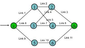
Figure 2: Wireless Network Scenario

There are five different paths, where the source node $s$ can allocate data traffic to send to destination node $d_{s}$. The paths $p_{sk}$ are

$$p_{s1} =\{(s,1),(1,2),(2,d_{s})\}$$

$$p_{s2} =\{(s,1),(1,4),(4,d_{s})\}$$

$$p_{s3} =\{(s,3),(3,2),(2,d_{s})\}$$

$$p_{s4} =\{(s,3),(3,4),(4,d_{s})\}$$

$$p_{s5} =\{(s,5),(5,6),(6,d_{s})\}$$

We define four trust update periods (each period is defined every $T_{update}$ time slots), in order to show the behavior of our approach for different trust values. For the simulations, we define $T_{update}=T/4=40$ time slots. Node trust estimates $\nu_{i}$ change dynamically at every update period, based on the trust evaluation mechanism. The different node trust values that we obtain from the trust evaluation mechanism for each of the four update periods are shown at the matrix below

$$\mathbf{\nu}=\bordermatrix{~{}&s&\text{1}&\text{2}&\text{3}&\text{4}&\text{5}&\text{6}&d_{s}\cr&1&1&1&0.7&1&0.7&0.5&1\cr&1&0.9&0.9&0.5&0.9&0.2&0.2&1\cr&1&0.9&0.9&0.3&0.7&0.1&0.1&1\cr&1&0.9&0.9&0.2&0.5&0.1&0.1&1\cr}$$ (27)

Trust values are adjusted using the EWMA algorithm expressed in Eq. (4), in order to prevent significant variations in the trust estimates over subsequent trust update periods. For our simulation, the EWMA algorithm uses $\alpha=0.8$ to give more significance to the latest update.

Given the trust values estimates in Matrix (27), we can notice that path $p_{s5}$ contains untrusted (malicious) nodes and should ideally be excluded from the traffic rate assignment. In addition, node $3$ is detected to be malicious and hence our mechanism should ideally assign significantly less traffic to the paths $p_{s3}$ and $p_{s4}$ that contain this node. Finally, node $4$ obtains a low trust value estimate at the last update period, which should lead to decrease in the traffic rate assignment even for path $p_{s2}$ that contains this node.

Figures 3(a) and 3(b) present the numerical results of the average traffic rate allocation for two different cases of maximum allowable traffic rate $\mathcal{R}_{s}$ (with the corresponding error bars). In the case of $\mathcal{R}_{s}=10$ kbps, the maximum traffic rate is close to the maximum allowable capacity of the wireless links, while in the case of $\mathcal{R}_{s}=14$ kbps, the maximum traffic rate is greater than the maximum capacity of the links. We observe that in both cases the traffic rate assigned to each routing path changes at every update period based on the trust estimates. Our algorithm assigns to the path $p_{s1}$ the maximum traffic rate, since it contains trusted nodes and to the path $p_{s5}$ the lowest traffic rate, because it consists of untrusted nodes. For the rest of the paths, the traffic rate is being adjusted according to trust estimates of every update period. We also observe that in the case of $\mathcal{R}_{s}=14$, more traffic rate is allocated to untrusted paths to cover the demand.

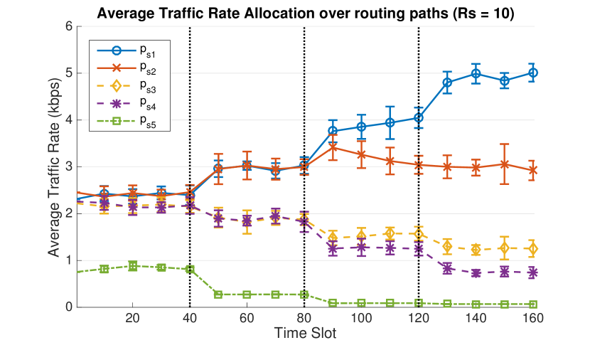
(a) Average Traffic Rate with $\mathcal{R}_{s}=10$

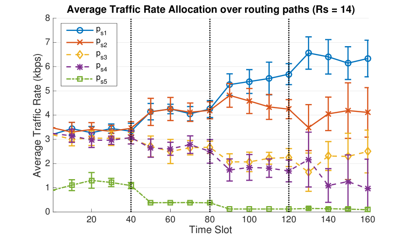
(b) Average Traffic Rate with $\mathcal{R}_{s}=14$

Figure 3: Average Traffic Rate over paths for different maximum rates $\mathcal{R}_{s}$

Link capacity margins $\sigma_{i,j}$ for some links of our wireless network, in the case of $\mathcal{R}_{s}=10$ and $\mathcal{R}_{s}=14$, are presented in Figure 4(a) and Figure 4(b) respectively. Link capacity margin is related with the average delay, since higher capacity margin indicates lower link delay and thus lower end-to-end delay. In our scenario, link $1$ has the lowest capacity margin, because our scheme allocates significantly high traffic rate to this link. In addition, we notice that links belonging to untrusted paths have high capacity link margin (e.g. link $7$ and $11$), since they do not relay high data traffic. We also observe that in the case of higher maximum data rate, the link margin takes lower values at the more congested links, because of the higher traffic rate that should be allocated. Links that belong to untrusted paths, such as link $5$, are being allocated more traffic rate in the case of higher data rate, in order to satisfy the underlying delay requirements. In general, the capacity margin is being adjusted in order to attain the delay constraints of the traffic flow, which in our scenario are being satisfied, even if our scheme has to reduce significantly the capacity margin of some wireless links.

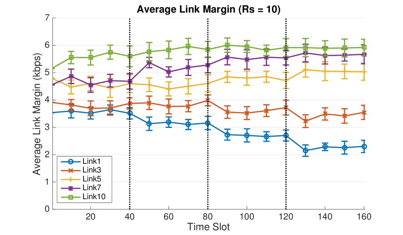
(a) Average Link Margin with $\mathcal{R}_{s}=10$

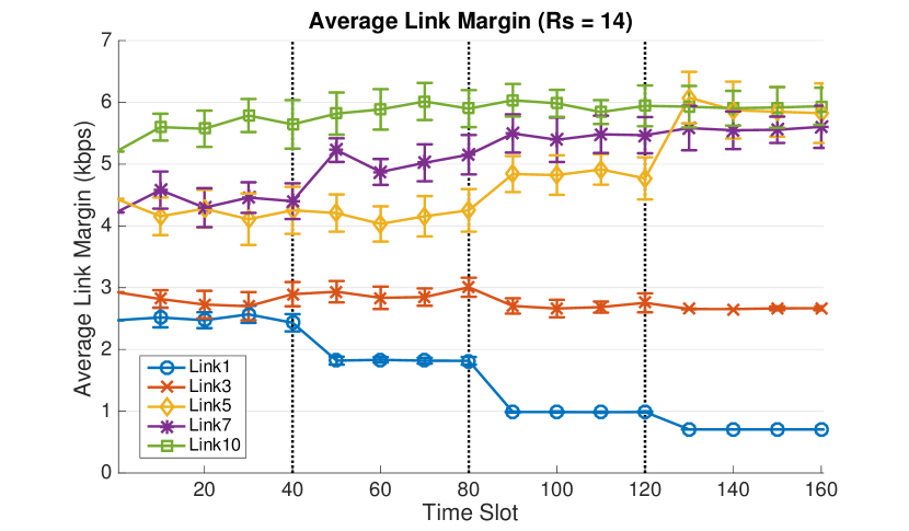
(b) Average Link Margin with $\mathcal{R}_{s}=14$

Figure 4: Average Link Margin in wireless links over time

VII Conclusion and Future Work

In this paper, we investigated an important application of performance and security tradeoff by introducing security considerations in the cross layer design of network protocols via network utility maximization (NUM). The specific concept of security we used is “trust”. Users get higher utility by transmitting data through nodes of higher trust values. Thus, trust values should be taken into account as parameters in the optimization problem, so that the resulting trust-aware protocols are resilient to network failures and to possible attacks. We also incorporated delay constraints in the utility optimization problem to capture QoS requirements. Finally, we proposed a distributed algorithm that achieves network utility maximization. As part of future work, we plan to investigate how dynamic changes in trust values affect the utility optimization problem, and to evaluate our approach in large scale scenarios.

References

- [1] M. Chiang, S. H. Low, A. R. Calderbank, and J. C. Doyle, “Layering as optimization decomposition: A mathematical theory of network architectures,” Proceedings of the IEEE, vol. 95, no. 1, pp. 255–312, January 2007.
- [2] L. Chen, S. Low, M. Chiang, and J. Doyle, “Cross-layer congestion control, routing and scheduling design in ad hoc wireless networks,” in Proceedings of the 25th IEEE International Conference on Computer Communications (INFOCOM), April 2006, pp. 1–13.
- [3] E. Stai, S. Papavassiliou, and J. Baras, “Performance-aware cross-layer design in wireless multihop networks via a weighted backpressure approach,” IEEE/ACM Transactions on Networking, vol. PP, no. 99, pp. 1–1, 2014.
- [4] L. Tassiulas and A. Ephremides, “Stability properties of constrained queueing systems and scheduling policies for maximum throughput in multihop radio networks,” IEEE Transaction on Automatic Control, vol. 37, no. 12, pp. 1936–1949, December 1992.
- [5] X. Lin, N. B. Shroff, and R. Srikant, “A tutorial on cross layer optimization in wireless networks,” IEEE Journal on Selected Areas in Communications, vol. 24, no. 8, pp. 1452–1463, August 2006.
- [6] G. Theodorakopoulos and J. Baras, “On trust models and trust evaluation metrics for ad hoc networks,” IEEE Journal on Selected Areas in Communications, vol. 24, no. 2, pp. 318–328, Feb 2006.
- [7] S. Marti, T. J. Giuli, K. Lai, and M. Baker, “Mitigating routing misbehavior in mobile ad hoc networks,” in Proceedings of the 6th Annual International Conference on Mobile Computing and Networking. Boston, Massachusetts, United States: ACM Press, 2000, pp. 255–265.
- [8] F. Qiu, J. Bai, and Y. Xue, “Towards optimal rate allocation in multi-hop wireless networks with delay constraints: A double-price approach,” in Proceedings of the IEEE International Conference on Communications (ICC), June 2012, pp. 5280–5285.
- [9] D. P. Palomar and M. Chiang, “A tutorial on decomposition methods for network utility maximization,” IEEE Journal on Selected Areas in Communications, vol. 24, no. 8, pp. 1439–1451, August 2006.
- [10] N. Trichakis, A. Zymnis, and S. Boyd, “Dynamic network utility maximization with delivery contracts,” in in Proceedings of the IFAC World Congress, 2008, pp. 2907–2912.
- [11] M. H. Hajiesmaili, M. S. Talebi, and A. Khonsari, “Utility-optimal dynamic rate allocation under average end-to-end delay requirements,” CoRR, vol. abs/1509.03374, 2015.
- [12] J. Baras, T. Jiang, and P. Purkayastha, “Constrained coalitional games and networks of autonomous agents,” in Proceedings of the 3rd International Symposium on Communications, Control and Signal Processing (ISCCSP), March 2008, pp. 972–979.
- [13] P. Tague, S. Nabar, J. Ritcey, and R. Poovendran, “Jamming-aware traffic allocation for multiple-path routing using portfolio selection,” IEEE/ACM Transactions on Networking, vol. 19, no. 1, pp. 184–194, Feb 2011.
- [14] J. Sherry, C. Lan, R. A. Popa, and S. Ratnasamy, “Blindbox: Deep packet inspection over encrypted traffic,” in Proceedings of the 2015 ACM Conference on Special Interest Group on Data Communication, ser. SIGCOMM, New York, NY, USA, pp. 213–226.
- [15] M. Blaze, J. Feigenbaum, J. Ioannidis, and A. D. Keromytis, “The role of trust management in distributed systems security,” Secure Internet Programming: Security Issues for Mobile and Distributed Objects, pp. 185–210, 1999.
- [16] L. Eschenauer, V. D. Gligor, and J. Baras, “On trust establishment in mobile ad-hoc networks,” in Proceedings of the Security Protocols Workshop. Springer-Verlag, 2002, pp. 47–66.
- [17] T. Jiang and J. Baras, “Trust credential distribution in autonomic networks,” in Proceedings of IEEE Global Telecommunications Conference (GLOBECOM), Nov 2008, pp. 1–5.
- [18] U. M. Maurer, “Modelling a public-key infrastructure,” in Proceedings of the 4th European Symposium on Research in Computer Security: Computer Security (ESORICS), London, UK, 1996, pp. 325–350.
- [19] S. W. Roberts, “Control chart tests based on geometric moving averages,” Technometrics, vol. 42, no. 1, pp. 97–101, 2000.
- [20] J.-W. Lee, M. Chiang, and A. Calderbank, “Price-based distributed algorithms for rate-reliability tradeoff in network utility maximization,” IEEE Journal on Selected Areas in Communications, vol. 24, no. 5, pp. 962–976, May 2006.
- [21] K. Jain, J. Padhye, V. N. Padmanabhan, and L. Qiu, “Impact of interference on multi-hop wireless network performance,” in Proceedings of the 9th Annual International Conference on Mobile Computing and Networking (MobiCom), New York, NY, USA, 2003, pp. 66–80.
- [22] S. Boyd and L. Vandenberghe, Convex Optimization. New York, NY, USA: Cambridge University Press, 2004.
- [23] D. P. Bertsekas, Nonlinear Programming. Belmont, MA: Athena Scientific, 1999.