Different definitions of conic sections
in hyperbolic geometry

Abstract.

In classical Euclidean geometry, there are several equivalent definitions of conic sections. We show that in the hyperbolic plane, the analogues of these same definitions still make sense, but are no longer equivalent, and we discuss the relationships among them.

1. Introduction

Throughout this paper, $\mathbb{E}^{n}$ will denote Euclidean $n$-space and $\mathbb{H}^{n}$ will denote hyperbolic $n$-space. Recall that (up to isometry) these are the unique complete simply connected Riemannian $n$-manifolds with constant curvature $0$ and $-1$, respectively. We will use $d(x,y)$ for the Riemannian distance between points $x$ and $y$ in either of these geometries. We will sometimes identify $\mathbb{E}^{n}$ with affine $n$-space $\mathbb{A}^{n}(\mathbb{R})$ over the reals, which can then be embedded as usual in projective $n$-space $\mathbb{P}^{n}(\mathbb{R})$ (the set of lines through the origin in $\mathbb{A}^{n+1}(\mathbb{R})$). While this paper is about $2$-dimensional geometry, we will sometimes need to consider the case $n=3$ as well as $n=2$.

1.1. Hyperbolic geometry

Hyperbolic geometry is a form of non-Euclidean geometry, which modifies Euclid’s fifth axiom, the parallel postulate. The parallel postulate has an equivalent statement, known as Playfair’s axiom.

Definition 1 (Playfair’s axiom).

Given a line $l$ and a point $p$ not on $l$, there exists only one line through $p$ parallel to $l$.

In hyperbolic geometry, this is modified by allowing an infinite number of lines through $p$ parallel to $l$. This has interesting effects, resulting in the angles in a triangle adding up to less than $\pi$ radians, and a relation between the area of the triangle and the angular defect, the difference between $\pi$ and the sum of the angles. Hyperbolic geometry may also be considered to be the Riemannian geometry of a surface of constant negative curvature. When this curvature is normalized to $-1$, there are especially nice formulas, such as the fact that the area of a triangle is equal to the angular defect.

However, since a surface of negative curvature cannot be embedded in a surface of zero curvature, hyperbolic geometry requires “models” to represent hyperbolic space on a flat sheet of paper. There are many such models, including the Poincaré disk and the Poincaré upper half-plane model. These all have varying metrics and methods of representing lines (i.e., geodesics) and shapes.

In the Poincaré disk model of $\mathbb{H}^{2}$, $\{z\in\mathbb{R}^{2}\mid|z|<1\}$, geodesics are either circular arcs orthogonal to the unit circle or else lines through the origin. The metric is defined as:

$$(ds)^{2}=\frac{(dx)^{2}+(dy)^{2}}{(1-x^{2}-y^{2})^{2}}.$$

In the upper half-plane model of $\mathbb{H}^{2}$, $\{(x,y)\in\mathbb{R}^{2}\mid y>0\}$, geodesics are either lines orthogonal to the $x$-axis or else circular arcs orthogonal to the $x$-axis. The metric is defined as:

$$(ds)^{2}=\frac{(dx)^{2}+(dy)^{2}}{y^{2}}.$$

In the Klein disk model or Beltrami-Klein model of $\mathbb{H}^{2}$, the points in the model are the points of the open unit disk in the Euclidean plane, and the geodesics are the intersection with the open disk of chords joining two points on the unit circle. The formula for the metric in this model is rather complicated:

$$(ds)^{2}=\frac{(dx)^{2}+(dy)^{2}}{1-x^{2}-y^{2}}+\frac{(x\,dx+y\,dy)^{2}}{(1-x^{2}-y^{2})^{2}}.$$

1.2. Conics

Definition 2.

One of the oldest notions in geometry, going all the way back to Apollonius, is that of conic sections in $\mathbb{E}^{2}$. There are at least four equivalent definitions of a conic section $C$:

1. a smooth irreducible algebraic curve in $\mathbb{A}^{2}(\mathbb{R})$ of degree $2$;

2. the intersection of a right circular cone in $\mathbb{E}^{3}$ (with vertex at the origin, say) with a plane not passing through the origin, this plane in turn identified with $\mathbb{E}^{2}$;

3. the two focus definition: Fix two points $a_{1},a_{2}\in\mathbb{E}^{2}$. An ellipse $C$ is the locus of points $x\in\mathbb{E}^{2}$ such that $d(x,a_{1})+d(x,a_{2})=c$, where $c>0$ is a fixed constant. Similarly, a hyperbola $C$ is the locus of points $x\in\mathbb{E}^{2}$ such that $\left|d(x,a_{1})-d(x,a_{2})\right|=c$, where $c>0$ is a fixed constant. The points $a_{1}$ and $a_{2}$ are called the foci of the conic, and the line joining them (assuming $a_{1}\neq a_{2}$) is called the major axis. A circle is the special case of an ellipse where $a_{1}=a_{2}$. A parabola is the limiting case of a one-parameter family of ellipses $C_{t}(a_{1},a_{2},c_{t})$ where $a_{1}$ is fixed and we let $a_{2}$ run off to infinity along the major axis keeping $c_{t}-d(a_{1},a_{2})$ fixed.

4. the focus/directrix definition: Fix a point $a_{1}\in\mathbb{E}^{2}$, called the focus, and a line $\ell$ not passing through $a_{1}$, called the directrix. A conic $C$ is the locus of points with $d(x,a_{1})=\varepsilon d(x,\ell)$, where $\varepsilon>0$ is a constant called the eccentricity. If $\varepsilon<1$ the conic is called an ellipse; if $\varepsilon=1$ the conic is called a parabola; if $\varepsilon>1$ the conic is called a hyperbola. A circle is the limiting case of an ellipse obtained by fixing $a_{1}$ and sending $\varepsilon\to 0$ and $d(a_{1},\ell)\to\infty$ while keeping $r=\varepsilon d(a_{1},\ell)$ fixed.

Note that these definitions come from totally different realms. Definition 2(1) is from algebraic geometry. Definition 2(2) uses a totally geodesic embedding of $\mathbb{E}^{2}$ into $\mathbb{E}^{3}$. Definitions 2(3) and 2(4) use only the metric geometry of $\mathbb{E}^{2}$.

Since Definition 2(1) is phrased in terms of algebraic geometry, it naturally leads to a definition of a conic in $\mathbb{P}^{2}(\mathbb{R})$ as a smooth irreducible algebraic curve of degree $2$. Such a curve must be given (in homogeneous coordinates) by a homogeneous quadratic equation $Q(x)=0$, where $Q$ is a nondegenerate indefinite quadratic form on $\mathbb{R}^{3}$. This is the equation of a cone, and intersecting the cone with an affine plane not passing through the origin (the vertex of the cone) gives us back Definition 2(2).

1.3. Contents of this paper

The topic of this paper is studying what happens to Definitions 2(1)–(4) when we replace $\mathbb{E}^{2}$ by $\mathbb{H}^{2}$. This is an old problem, and is discussed for example in [9, 3, 6, 7, 8]. However, as we will demonstrate, the analogues of Definitions 2(1)–(4) are no longer equivalent in $\mathbb{H}^{2}$. Thus there is some confusion in the literature, and those who talk about conic sections in $\mathbb{H}^{2}$ (as recently as [4, 5]) do not always all mean the same thing. Our main results are Theorems 11, 13, 14, and 15 in Section 3, which clarify the relationships among these definitions (especially the two-focus and focus-directrix definitions) in $\mathbb{H}^{2}$. Table 1 summarizes our results.

Circles

3 $\Leftrightarrow$ 7. 3, 7 included in 4, 6. 3, 7 $\not\Leftrightarrow$ 8.

Horocycles (paracycles), hypercycles

included in 5, 6. not included in 7, 8.

Ellipses

7 $\not\Leftrightarrow$ 8. But when 8 gives a closed curve, it is included in 7.

Hyperbolas

7 $\subsetneqq$ 8.

Parabolas

7 $\not\Leftrightarrow$ 8. Neither kind of parabola is ever closed.

Table 1. Relationships among possible definitions of conics in $\mathbb{H}^{2}$. Numbers refer to the numbered definitions in sections 2 and 3.

2. Other Axiomatizations

Before discussing conics in $\mathbb{H}^{2}$, we first explain still another definition of conic sections in $\mathbb{P}^{2}(\mathbb{R})$, which is the definition found in [3, Ch. III] and with a slight variation in [9]. This definition uses the notion of a polarity $p$ in $\mathbb{P}^{2}(\mathbb{R})$. This is a particular type of mapping of points to lines and lines to points preserving the incidence relations of projective geometry (or in the language of [3, §3.1], a correlation). It can be explained in terms of algebraic geometry as follows. If $Q$ is a nondegenerate quadratic form on $\mathbb{R}^{3}$, then there is an associated nondegenerate symmetric bilinear form defined by $B(x,y)=(Q(x+y)-Q(x)-Q(y))/2$, and if $V$ if a linear subspace of $\mathbb{R}^{3}$ of dimension $d=1$ or $2$, then the orthogonal complement $V^{\perp,B}$ of $V$ with respect to $B$ is a linear subspace of dimension $3-d$. Thus the process $p$ of taking orthogonal complements with respect to $B$ sends points in $\mathbb{P}^{2}(\mathbb{R})$, which are $1$-dimensional linear subspaces of $\mathbb{R}^{3}$, to lines (copies of $\mathbb{P}^{1}(\mathbb{R})$), which are $2$-dimensional linear subspaces of $\mathbb{R}^{3}$, and vice versa. Given a polarity $p$, the associated conic is the set $C$ of points $x\in\mathbb{P}^{2}(\mathbb{R})$ such that $x$ lies on the line $p(x)$, i.e., the set of $1$-dimensional linear subspaces $V$ of $\mathbb{R}^{3}$ for which $V\subset V^{\perp,B}$, or in other words, for which $V$ is $B$-isotropic. Thus if we identify the point $x\in\mathbb{P}^{2}(\mathbb{R})$ with its homogeneous coordinates, or with a basis vector for $V$ up to rescaling, this becomes the condition $B(x,x)=0$, or $Q(x)=0$, which is just Definition 2(1). (Note that if $Q$ is definite, the conic is empty, so we are forced to take $Q$ to be indefinite in order to get anything interesting.) Conversely, it is well known [3, §4.72] that every polarity arises from a nonsingular symmetric matrix or equivalently from a nondegenerate quadratic form $Q$, so the polarity definition of conics in [3, Ch. III] is equivalent to Definition 2(1).

We now introduce several possible definitions of conic sections in $\mathbb{H}^{2}$.

Definition 3 (A metric circle).

A circle in $\mathbb{H}^{2}$ is the locus of points a fixed distance $r>0$ from a center $x_{1}\in\mathbb{H}^{2}$, i.e., $C=\{x\in\mathbb{H}^{2}:d(x,x_{1})=r\}$.

Definition 4 (Analogue of Definition 2(2)).

A right circular cone in $\mathbb{H}^{3}$ is defined as follows. Fix a point $x_{0}\in\mathbb{H}^{3}$ (say the origin, if we are using the standard unit ball in $\mathbb{R}^{3}$ as our model of $\mathbb{H}^{3}$) and fix a plane $P$ in $\mathbb{H}^{3}$ (a totally geodesic copy of $\mathbb{H}^{2}$) not passing through $x_{0}$. There is a unique ray starting at $x_{0}$ and intersecting $P$ perpendicularly. Let $x_{1}$ be the intersection point (the closest point on $P$ to $x_{0}$), and fix a radius $r>0$. We then have the circle $C$ in $P$ centered at $x_{1}$ with radius $r$. The cone $c(x_{0},C)$ through $x_{0}$ and $C$ is then the union of the lines (geodesics) through $x_{0}$ passing through a point of $C$. The point $x_{0}$ is called the vertex of the cone. A conic section (in the literal sense!) in $\mathbb{H}^{2}$ is then the intersection of a plane $P^{\prime}$ in $\mathbb{H}^{3}$ (not passing through $x_{0}$) with $c(x_{0},C)$.

Since we can take $P^{\prime}=P$ in the above definition, it is obvious that a circle (as in Definition 3) is a special case of a conic section in the sense of Definition 4.

In the Poincaré ball model of $\mathbb{H}^{3}$ with $x_{0}$ the origin, geodesics through $x_{0}$ are just straight lines for the Euclidean metric, so it’s easy to see that a right circular cone with vertex $x_{0}$ is also a right circular cone in the Euclidean sense in $\mathbb{R}^{3}$. On the other hand, planes in $\mathbb{H}^{3}$ not passing through $x_{0}$ correspond to Euclidean spheres perpendicular to the unit sphere (the boundary of the model of $\mathbb{H}^{3}$). Thus a conic section in the sense of Definition 4 is the intersection of a right circular cone with a sphere, and is thus (in terms of the algebraic geometry of $\mathbb{A}^{3}(\mathbb{R})$) an algebraic curve of degree $\leq 4$. To view this conic in the usual Poincaré disk model of $\mathbb{H}^{2}$, we apply an isometry (stereographic projection) from $P$ to the unit disk in $\mathbb{C}$. Since this is a rational map, we see that any conic section in the sense of Definition 4 is an algebraic curve (in fact of degree $\leq 4$) when viewed in the disk model of $\mathbb{H}^{2}$. Alternatively, if we use the Klein ball model of $\mathbb{H}^{3}$ with $x_{0}$ the origin, then a right circular cone with vertex $x_{0}$ will again look like a Euclidean right circular cone, while a $2$-plane in $\mathbb{H}^{3}$ will be the intersection of the ball with a Euclidean $2$-plane, and any conic section in the sense of Definition 4 will also be a conic section in the Euclidean sense of Definition 2. Thus Definition 4 is equivalent to the following Definition 5.

Definition 5 (Analogue of Definition 2(1)).

A conic in $\mathbb{H}^{2}$ in the algebraic sense is the intersection of a smooth irreducible algebraic curve of degree $2$ in $\mathbb{A}^{2}(\mathbb{R})$ with the open unit disk, viewed as the Klein disk model for $\mathbb{H}^{2}$. (This is a non-conformal model in which points of $\mathbb{H}^{2}$ are points of the open unit disk, and the straight lines are intersections with the open disk of straight lines in the plane.) Such a conic is closed (compact) if and only if it is a circle or ellipse not intersecting the unit circle (the absolute in the terminology of [9] and [3]).

Definition 5 is the definition of conics used in [9] and [3].

Still another approach to defining conics may be found in [8], based on the axiom system for $\mathbb{E}^{2}$ and $\mathbb{H}^{2}$ developed in [2]. First we need to discuss Bachmann’s approach to metric geometry. Bachmann observes that in either $\mathbb{E}^{2}$ and $\mathbb{H}^{2}$, there is a unique isometry which is reflection in a given line $a$ or around a given point $A$. Thus we can identify lines and points with certain distinguished involutory elements $\mathcal{S}$ (the reflections in lines) and $\mathcal{P}$ (the reflections around points) of the isometry group $G$. More is true: every element of $G$ is a product of at most three elements of $\mathcal{S}$. Elements of $\mathcal{S}$ are orientation-reversing; elements of $\mathcal{P}$ are orientation-preserving. The product of two elements $a,\,b\in\mathcal{S}$ is a non-trivial involution if and only if $a\neq b$ and $ab=ba$; in this case, the lines associated to $a$ and $b$ are perpendicular (we write $a\perp b$) and $ab\in\mathcal{P}$ is the reflection around the unique intersection point of $a$ and $b$. Furthermore, every element of $G$ of order $2$ belongs to $\mathcal{S}$ or to $\mathcal{P}$, but not to both. A point $A\in\mathcal{P}$ lies on a line $a\in\mathcal{S}$ exactly when there exists $b\in\mathcal{S}$ commuting with $a$ such that $A=ab$. Thus a metric plane $\mathcal{M}$ can be identified with a group $G$ together with a distinguished generating set $\mathcal{S}$ consisting of involutions and the set $\mathcal{P}$ of non-trivial products of commuting elements of $\mathcal{S}$, satisfying certain axioms. We won’t need the axioms here, since they will be evident in the cases we are interested in. In the case of $\mathbb{E}^{2}$, $G=\mathbb{R}^{2}\rtimes O(2)$, the usual Euclidean motion group, and in the case of $\mathbb{H}^{2}$, $G=PGL(2,\mathbb{R})\cong O^{+}(2,1)$. (If $\begin{pmatrix}a&b\\ c&d\end{pmatrix}$ has determinant $+1$, then it operates on the upper half-plane by linear fractional transformations, which are orientation-preserving, and if it has determinant $-1$, then it operates on the upper half-plane by

$$z\mapsto\frac{a\bar{z}+b}{c\bar{z}+d},$$

and this conjugate-linear map is an orientation-reversing isometry of $\mathbb{H}^{2}$.)

Bachmann also points out that the metric plane $(\mathcal{M},\mathcal{S},\mathcal{P})$ corresponding to $\mathbb{E}^{2}$ or $\mathbb{H}^{2}$ can be embedded naturally in a projective-metric plane $(\mathcal{P}\mathcal{M},\mathcal{S}^{\prime},\mathcal{P}^{\prime})$, in such a way that $\mathcal{S}\subseteq\mathcal{S}^{\prime}$ and $\mathcal{P}\subseteq\mathcal{P}^{\prime}$. In the case of $\mathbb{E}^{2}$, this is just the usual embedding of $\mathbb{A}^{2}(\mathbb{R})$ in $\mathbb{P}^{2}(\mathbb{R})$ by adjoining a copy of $\mathbb{P}^{1}(\mathbb{R})$ at $\infty$, and the associated group is $PGL(3,\mathbb{R})$. In the case of $\mathbb{H}^{2}$, $\mathcal{P}\mathcal{M}$ is again a copy of $\mathbb{P}^{2}(\mathbb{R})$, but its points and lines consist of ideal points and ideal lines of $\mathbb{H}^{2}$. A simple way to visualize the embedding of $\mathbb{H}^{2}$ in $\mathbb{P}^{2}(\mathbb{R})$ is to use the (non-conformal) Klein model of $\mathbb{H}^{2}$, in which points are points in the interior of the unit disk in $\mathbb{R}^{2}$, and lines are the intersections of ordinary straight lines in $\mathbb{A}^{2}(\mathbb{R})$ with the unit disk. Then each point or line of $\mathbb{H}^{2}$ obviously corresponds to a unique point or line of $\mathbb{P}^{2}(\mathbb{R})$. When viewed as $\mathcal{P}\mathcal{M}$ in this way, $\mathbb{P}^{2}(\mathbb{R})$ carries a canonical polarity, namely the one associated to the unit circle in $\mathbb{A}^{2}(\mathbb{R})$, viewed as a conic in the sense of the polarity definition at the beginning of this Section. When we embed $\mathbb{A}^{2}(\mathbb{R})$ in $\mathbb{P}^{2}(\mathbb{R})$ as usual via $(x,y)\mapsto[x,y,1]$ (homogeneous coordinates denoted by square brackets), this polarity is associated to the quadratic form $Q\colon\,(x,y,z)\mapsto x^{2}+y^{2}-z^{2}$, since $Q(\cos\theta,\sin\theta,1)=0$ for any real angle $\theta$.

Definition 6 ([8, Definition 4.1]).

A conic $C$ in the sense of Molnár, with foci $A,\,B\in\mathbb{P}^{2}(\mathbb{R})$, is defined by choosing a line $x_{1}$ in $\mathbb{P}^{2}(\mathbb{R})$ which is not a boundary line (i.e., $x_{1}$ is not tangent to the unit circle) and not passing through either $A$ or $B$, and with $A$ and $B$ not each other’s reflections across $x_{1}$. Then $C$ consists of points $X_{11}$ and $X$ chosen as follows. $X_{11}$ is the intersection of the lines $a_{11}$ through $A$ and $B^{x_{1}}$ (the reflection of $B$ across $x_{1}$) and $b_{11}$ through $B$ and $A^{x_{1}}$. (The line $x_{1}$ is chosen so that $a_{11}$ and $b_{11}$ are not boundary lines.) The other points $X$ are defined by fixing a point $Y$ on $x_{1}$ and taking the lines $a$ through $Y$ and $A$ and $b$ though $Y$ and $B$, and then if neither $a$ nor $b$ is a boundary line, letting $X$ be the intersection of $a_{11}^{a}$ and $b_{11}^{b}$ (the reflections of $a_{11}$ and $b_{11}$ across $a$ and $b$, respectively). Appropriate modifications are made if $a$ or $b$ is a boundary line.

As is quite evident, Molnár’s definition is quite complicated but results in a conic section in $\mathbb{H}^{2}$ being the intersection of a conic in $\mathbb{P}^{2}(\mathbb{R})$ with the unit disk (in the Klein model). We will not consider this definition further, but it’s closely related to Definition 5. A picture of the construction with $A=(0,0)$, $B=(.5,0)$, $x_{1}=\{y=.5\}$ is shown in Figure 1.

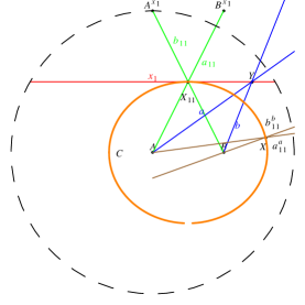
Figure 1. Molnár’s construction of a conic

3. Main Results

Definition 7 (Analogue of Definition 2(3)).

The definition of two focus conics in Definition 2(3) immediately goes over to $\mathbb{H}^{2}$, simply by replacing the Euclidean distance by the hyperbolic distance. Note that the case of a circle was already mentioned in Definition 3.

The last definition is the only one that is not immediately obvious. However, if were we to carry Definition 2(4) over to $\mathbb{H}^{2}$ without change, then since in the upper half-plane or disk models of $\mathbb{H}^{2}$, the distance function is the log of an algebraic expression, in the case of irrational eccentricity $\varepsilon$ we would effectively get the equation

$$(\text{algebraic expression})=(\text{algebraic expression})^{\varepsilon},$$

which is a transcendental equation, and could not possibly agree with the other definitions of conic sections. This explains the modification made in [9]. The use of the hyperbolic sine comes from its role in hyperbolic geometry via the solution of the Jacobi equation.

Definition 8.

[Analogue of Definition 2(4)] Fix a point $a_{1}\in\mathbb{H}^{2}$, called the focus, and a line (geodesic) $\ell$ not passing through $a_{1}$, called the directrix. A conic $C$ is the locus of points $x\in\mathbb{H}^{2}$ with $\sinh d(x,a_{1})=\varepsilon\sinh d(x,\ell)$, where $\varepsilon>0$ is a constant called the eccentricity. If $\varepsilon<1$ the conic is called an ellipse; if $\varepsilon=1$ the conic is called a parabola; if $\varepsilon>1$ the conic is called a hyperbola. (Note: in the case of the parabola, but only in this case, the hyperbolic sines cancel and can be removed from the definition.) A circle is the limiting case of an ellipse obtained by fixing $a_{1}$ and sending $\varepsilon\to 0$ and $d(a_{1},\ell)\to\infty$ while keeping $r=\varepsilon\sinh d(a_{1},\ell)$ fixed.

3.1. Circles

We begin now to compare the various definitions. We start with the circle, which is the most straightforward. Definition 3 clearly coincides with Definition 4, in the sense that if we intersect a right circular cone with a plane perpendicular to the axis, the result is a circle in the sense of Definition 3. We also have the following.

Proposition 9.

Definition 3 coincides with the case of circles in Definition 5, but with the Klein model replaced by the Poincaré model. In other words, an ordinary circle in $\mathbb{A}^{2}(\mathbb{R})$, contained in the open unit disk, when viewed as a curve in the Poincaré disk model of $\mathbb{H}^{2}$ is a metric circle in $\mathbb{H}^{2}$, and vice versa. Similarly, an ordinary circle contained in the upper half-plane, when viewed as a curve in the Poincaré upper half-plane model of $\mathbb{H}^{2}$, is a metric circle in $\mathbb{H}^{2}$, and vice versa.

Proof.

First consider the disk model. If the center is the origin, this is clear since the hyperbolic distance from $0$ to $z$ in $\{z:|z|<1\}$ in $\mathbb{C}$ is a (nonlinear) function $\tanh^{-1}(|z|)=\frac{1}{2}\log\bigl{(}\frac{1+|z|}{1-|z|}\bigr{)}$ of the Euclidean distance $|z|$ from $0$ to $z$, so that each Euclidean circle centered at $0$ is also a hyperbolic circle (of a different radius), and vice versa. However, any circle in $\mathbb{H}^{2}$ can be mapped to a circle centered at $0$ via an isometry of $\mathbb{H}^{2}$, and since linear fractional transformations send circles to circles [1, Ch. 3, §3.2, Theorem 14], the general case follows. The case of the half-plane model also follows since there is a linear fractional transformation relating this model to the disk model. ∎

Remark 10.

However, one should note that the center of a circle in the unit disk or the upper half-plane may differ, depending on whether one considers it as a Euclidean circle or a metric circle in $\mathbb{H}^{2}$. For example, the metric circle in $\mathbb{H}^{2}$ (in the upper-halfplane model) around the point $i$ with hyperbolic metric radius $\log 2$ has Euclidean equation

$$\frac{|z-i|}{|z+i|}=\tanh\left(\frac{1}{2}\,\log 2\right)=\frac{1}{3}\text{ or }\left|z-\frac{5}{4}i\right|=\frac{3}{4},$$

so its center as a Euclidean circle is $\frac{5}{4}\,i$.

Metric circles in $\mathbb{H}^{2}$, when drawn in the Klein disk model, only appear to be circles when centered at the origin. Otherwise, they are ellipses.

However, the focus/directrix definition of circles is quite different.

Theorem 11.

The definition of circle in Definition 8 does not agree with the definition of circle in Definitions 3, 4, 5, and 7.

Proof.

Consider a circle in the sense of Definition 8. Without loss of generality, we work in the upper half-plane model of $\mathbb{H}^{2}$ and set $a_{1}=i$, $\ell=\{z\in\mathbb{H}^{2}:|z|=R\}$, where we let $R\to+\infty$. In this case $d(a_{1},\ell)=\log R$ and we want to keep $r=\varepsilon\sinh(\log R)=\frac{\varepsilon(R^{2}-1)}{2R}$ constant, so we take $\varepsilon=\frac{2rR}{R^{2}-1}$. For $z\in\mathbb{H}^{2}$,

$$d(z,\ell)=\tfrac{1}{2}\,d(z,w),\text{ where }w=\frac{R^{2}}{\overline{z}}=\text{reflection of }z\text{ across }\ell.$$

Then the equation $\sinh d(z,a_{1})=\varepsilon\sinh d(z,\ell)$ becomes

$$\sinh\left(2\tanh^{-1}\left|\frac{z-i}{z+i}\right|\right)=\frac{2rR}{R^{2}-1}\sinh\left(\tanh^{-1}\left|\frac{z-\frac{R^{2}}{\overline{z}}}{z-\frac{R^{2}}{z}}\right|\right).$$

The left-hand side simplifies to

$$\frac{2|z+i|\,|z-i|}{|z+i|^{2}-|z-i|^{2}}=\frac{|z^{2}+1|}{2\operatorname{Im}z}.$$

On the right-hand side,

$$\left|\frac{z-\frac{R^{2}}{\overline{z}}}{z-\frac{R^{2}}{z}}\right|=\frac{R^{2}-|z|^{2}}{\left|R^{2}-|z|^{2}\frac{z}{\overline{z}}\right|}=\frac{R^{2}-a}{\sqrt{R^{4}+a^{2}-2R^{2}a\cos(\theta)}}$$

where $a=|z|^{2}$ and $\theta=2\arg z$. Then

$$\lim_{R\to\infty}\frac{2rR}{R^{2}-1}\sinh\left(\tanh^{-1}\left(\frac{R^{2}-a}{\sqrt{R^{4}+a^{2}-2R^{2}\cos(\theta)}}\right)\right)=\frac{\sqrt{2}r}{|z|\sqrt{1-\cos(\theta)}}.$$

Thus Definition 8 gives for our circle the equation

$$\frac{|z^{2}+1|}{2\operatorname{Im}z}=\frac{\sqrt{2}r}{|z|\sqrt{1-\cos(\theta)}}=\frac{r}{|z|}\csc(\theta/2)=\frac{r}{|z|}\frac{|z|}{\operatorname{Im}z}=\frac{r}{\operatorname{Im}z},$$

or

(1) $$|z^{2}+1|={2r}.$$

in the upper half-plane. This is an algebraic curve but not a metric circle. Figure 2 shows the case of $r=.25$ (in solid color) as drawn with Mathematica. This curve passes through the points $i\sqrt{\frac{3}{2}}$, $i\sqrt{\frac{1}{2}}$, and $i\pm\sqrt{\frac{\sqrt{17}-4}{2}}$; the circle centered on the imaginary axis tangent to it at $i\sqrt{\frac{3}{2}}$ and $i\sqrt{\frac{1}{2}}$ is shown with a dashed line in the same figure. The curves are close but do not coincide. ∎

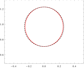
Figure 2. A “circle” with focus $i$ and $r=.25$ (solid color) and a tangent metric circle (dashed) in the upper half-plane

Aside from circles, there are various other circle-like curves that play a role in hyperbolic geometry. These may be considered to be conics according to certain definitions. Note also that they are distinct from the circles of Definition 8.

Definition 12.

A horocycle (occasionally called a paracycle) in the Poincaré disk model of $\mathbb{H}^{2}$ is the intersection of the disk with a circle tangent to the unit circle (and lying inside the circle). A hypercycle in the Poincaré disk model of $\mathbb{H}^{2}$ is the intersection of the disk with a circle meeting the unit circle in exactly two points. These have well-known intrinsic definitions. A horocycle is the limit of a sequence of circles $C_{n}$ (in the sense of Definition 3) all passing through a fixed point $x_{0}$, with centers $x_{n}$ all lying on a fixed ray through $x_{0}$ and with radii $d(x_{n},x_{0})=r_{n}\to\infty$. See Figure 3(a). A hypercycle is a curve on one side of a given line $\ell$ whose points all have the same orthogonal distance from $\ell$. See Figure 3(b). Note that horocycles and hypercycles are clearly conics in the sense of Definition 5. But they are not covered by Definitions 7 and 8. Molnár observes in [8] that metric circles (Definition 3), horocycles, and hypercycles are all special cases of Definition 6 when the two foci coincide.

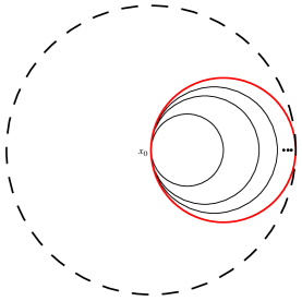
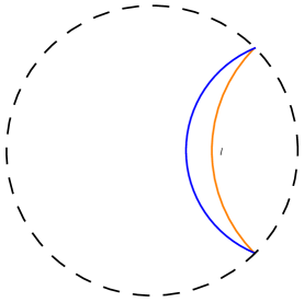
Figure 3. (a) (left) A horocycle (solid red) as a limit of circles (black) through $x_{0}$ with radii going to infinity. (b) (right) A hypercycle (solid blue) and a straight line $\ell$ (orange) with the same ideal limits at infinity

3.2. Ellipses

Next, we consider the case of the (noncircular) ellipse. There are two main competing definitions: Definition 7 and Definition 8.

Theorem 13.

The definition of ellipse in Definition 8 does not always agree with the definition of ellipse in Definition 7. However, there are cases where they coincide. More precisely, when Definition 8 gives a closed curve in $\mathbb{H}^{2}$, this curve is also a two-focus ellipse.

Proof.

We will work in the upper half-plane model of $\mathbb{H}^{2}$ and, without loss of generality, put one focus at $i$ and let the imaginary axis be an axis of the ellipse. For an ellipse with the “two-focus definition” and foci at $i$ and $bi$, $b>0$, the equation is

$$2\tanh^{-1}\left({\frac{|z-i|}{|z+i|}}\right)+2\tanh^{-1}\left({\frac{|z-bi|}{|z+bi|}}\right)=c,$$

which can be rewritten as the algebraic equation

(2) $$\left(x^{2}+y^{2}+1+\sqrt{(x^{2}-y^{2}+1)^{2}+4x^{2}y^{2}}\right)\\ \times\left(x^{2}+y^{2}+b^{2}+\sqrt{(x^{2}-y^{2}+b^{2})^{2}+4x^{2}y^{2}}\right)=4be^{c}\,y^{2}$$

with $c>0$. Plots of this equation for $b=\frac{3}{4}$ and for various values of $c$ are shown in Figure 4. The minimal value of $c$ to have the foci inside the ellipse is the hyperbolic distance between the foci, or $|\log b|$. As $c$ increases, the curves get bigger and bigger and look more like circles. Now that since (2) implies that $d(z,i)\leq c$, any ellipse in the sense of Definition 7 is automatically compact (closed) in $\mathbb{H}^{2}$.

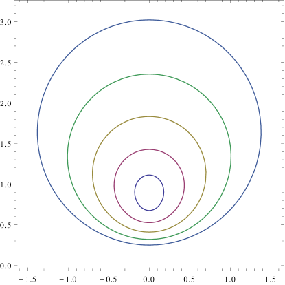
Figure 4. Two-focus ellipses in the upper half-plane with foci at $i$ and $\frac{3i}{4}$, as drawn with Mathematica

Now consider the focus-directrix definition for an ellipse in the upper half-plane, with a focus at $i$ and directrix $|z|=r$, $r>1$ (this choice makes the imaginary axis an axis of the ellipse). The distance from $z$ to the directrix is half the distance to the reflection of $z$ across the directrix, which is $\frac{r^{2}}{\overline{z}}$. Thus the equation becomes

$$\sinh\left(2\tanh^{-1}\left({\frac{|z-i|}{|z+i|}}\right)\right)=\varepsilon\,\sinh\left(\tanh^{-1}\left(\frac{\left|z-\frac{r^{2}}{\overline{z}}\right|}{\left|z-\frac{r^{2}}{z}\right|}\right)\right),$$

which simplifies (after squaring both sides) to

(3) $$r^{2}\left(1+x^{4}+y^{4}+2y^{2}\left(-1+\varepsilon^{2}\right)+2x^{2}\left(1+y^{2}+\varepsilon^{2}\right)\right)\\ =\varepsilon^{2}\,\left(r^{4}+\left(x^{2}+y^{2}\right)^{2}\right).$$

This is a relatively simple quartic equation in $x$ and $y$, basically the Cassini oval equation, and has some interesting features. For example, if one sets $\varepsilon=\frac{1}{r}$, this reduces to a lemniscate passing through $(0,0)$ (an ideal boundary point of $\mathbb{H}^{2}$). When $\varepsilon>\frac{1}{r}$, the curve (viewed in $\mathbb{H}^{2}$) is not closed and approaches two distinct ideal boundary points. Pictures of this behavior appear in Figure 5. As a check that having two distinct ideal boundary points is not just an artifact of the calculation, one can check that upon substituting $r=3$ and $\varepsilon=\frac{1}{2}$ into (3), one gets two points with $y=0$, namely $x=\pm\sqrt{\frac{3}{7}}$.

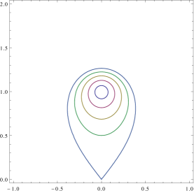
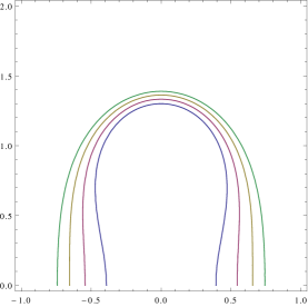
Figure 5. Focus/directrix ellipses in the upper half-plane with focus at $i$ and directrix $|z|=2$, as drawn with Mathematica. On the left, cases with $\varepsilon\leq.5$. The case $\varepsilon=.5$ is a lemniscate. On the right, cases with $\varepsilon$ from $.6$ to $.9$.

To illustrate another difference between the two definitions, consider the case of the two-focus definition when the foci coincide, i.e., $b=1$ in equation (2). Then equation (2) reduces to

$$x^{2}+y^{2}+1+\sqrt{(x^{2}-y^{2}+1)^{2}+4x^{2}y^{2}}=2e^{c/2}y$$

or

$$(x^{2}-y^{2}+1)^{2}+4x^{2}y^{2}-(2e^{c/2}y-x^{2}-y^{2}-1)^{2}=0,$$

which simplifies to the equation of a circle:

(4) $$x^{2}+\left(y-\cosh(c/2)\right)^{2}=\sinh^{2}(c/2).$$

However, the focus/directrix equation (3) never reduces to a circle.

However, perhaps rather surprisingly, focus/directrix ellipses with $\varepsilon<\frac{1}{r}$ (this is the case where the curve is closed) turn out to be special cases of two-focus ellipses. A rather horrendous calculation with Mathematica or MuPAD shows for example that (2) with $b=2$ and $c=\log\left(\frac{5}{2}\right)$ is equivalent to (3) with

$$\varepsilon=\frac{\sqrt{209}}{21},\quad r=\sqrt{\frac{11}{19}}.$$

To see this, rewrite (3) in the form

$$x^{2}+y^{2}+1 +\sqrt{(x^{2}-y^{2}+1)^{2}+4x^{2}y^{2}}$$

$$=\frac{20y^{2}}{x^{2}+y^{2}+4+\sqrt{(x^{2}-y^{2}+4)^{2}+4x^{2}y^{2}}}$$

$$=\frac{20y^{2}\left(x^{2}+y^{2}+4-\sqrt{(x^{2}-y^{2}+4)^{2}+4x^{2}y^{2}}\right)}{(x^{2}+y^{2}+4)^{2}-((x^{2}-y^{2}+4)^{2}+4x^{2}y^{2})},$$

simplify, and rewrite in the form $E+\sqrt{B}=F\sqrt{D}$, where $B=(x^{2}-y^{2}+1)^{2}+4x^{2}y^{2}$ and $D=(x^{2}-y^{2}+4)^{2}+4x^{2}y^{2}$. Square both sides, again simplify and regroup to get the term with $\sqrt{B}$ by itself, and finally square again. After factoring out $y^{2}$, one finally ends up with the equation

$$20x^{4}+40x^{2}y^{2}+325x^{2}+20y^{4}-116y^{2}+80=0,$$

which is equivalent to (3) for the given parameters. Other values of $r$ and $\varepsilon$ (with $r\varepsilon<1$) can be handled similarly; one just needs to solve for the values of $b$ and $c$ giving the same $y$-intercepts. ∎

3.3. Parabolas

Next, we consider the case of the parabola. Here the result is rather simple:

Theorem 14.

The definitions of parabolas in Definition 8 and in Definition 7 never agree. In all cases, however, a parabola in $\mathbb{H}^{2}$ is not closed.

Proof.

Without loss of generality, we can again use the Poincaré upper half-plane model of $\mathbb{H}^{2}$ and put one focus at $i$ and take the axis of the parabola to be the imaginary axis. The two-focus definition of Definition 7 is the limiting case of (2) as we keep $be^{c}=C/2$ fixed and let $b\to 0_{+}$. (This is because $d(i,ib)=|\log b|=-\log b$ for $0<b<1$ and we want $c-d(i,ib)=c+\log b$ to be held constant.) Then (2) reduces to

(5) $$\left(x^{2}+y^{2}+1+\sqrt{(x^{2}-y^{2}+1)^{2}+4x^{2}y^{2}}\right)\left(x^{2}+y^{2}\right)=C\,y^{2},$$

or equivalently (after regrouping and squaring to get rid of the radical, then factoring out a $y^{2}$)

(6) $$2(C-2)(x^{2}+y^{2})^{2}+2C(x^{2}+y^{2})-C^{2}y^{2}=0.$$

This is the equation of a lemniscate through the origin. (Remember that $0$, however, is only an ideal boundary point of $\mathbb{H}^{2}$.) Definition 8 simply gives (3) with $\varepsilon=1$, which reduces to

(7) $$1-r^{2}+4x^{2}+\left(1-\tfrac{1}{r^{2}}\right)(x^{2}+y^{2})^{2}=0,$$

which is a Cassini oval equation. Note that (6) and (7) never agree, since for $r\neq 1$ (we don’t want the directrix of the parabola to pass through the focus), the curve given by (7) doesn’t pass through the origin. Pictures of the various kinds of parabolas, plotted by Mathematica, are shown in Figures 6 and 7. ∎

Figure 6. Focus/directrix parabolas in the upper half-plane with focus at $i$ and directrix $|z|=r$, as drawn with Mathematica. On the left, cases with $r<1$. These are Cassini ovals. On the right, cases with $r>1$. Of course, if one were wearing “hyperbolic glasses,” all would look roughly the same.

Figure 7. Two-focus parabolas in the upper half-plane with focus at $i$, as drawn with Mathematica. Note the lemniscate shape.

3.4. Hyperbolas

Finally, we consider the case of the hyperbola.

Theorem 15.

The definition of hyperbola in Definition 8 does not always agree with the definition of hyperbola in Definition 7. However, the two-focus hyperbola from Definition 7 is a special case of the focus-directrix hyperbola of Definition 8.

Proof.

Consider the two-focus hyperbola. Fix $c>0$. (When $c=0$, the definition degenerates to the bisector of the line segment joining the two foci, which is a straight line (i.e., a geodesic).) We will work in the upper half-plane model of $\mathbb{H}^{2}$ and, without loss of generality, put one focus at $i$ and the other focus at $ib$, $b>1$. The equation of the two-focus hyperbola is then

$$2\tanh^{-1}\left({\frac{|z-i|}{|z+i|}}\right)-2\tanh^{-1}\left({\frac{|z-bi|}{|z+bi|}}\right)=\pm c,$$

which can be rewritten as the algebraic equation

(8) $$b^{2}+x^{2}+y^{2}+\sqrt{b^{4}+2b^{2}(x^{2}-y^{2})+(x^{2}+y^{2})^{2}}=\\ be^{\pm c}\left(1+x^{2}+y^{2}+\sqrt{1+2(x^{2}-y^{2})+(x^{2}+y^{2})^{2}}\right)$$

with $c>0$. Note that the hyperbola should intersect its axis (here the imaginary axis) at two points of the form $iy$, $1<y<b$, so we want $0<c<\log b$, and the two $y$-intercepts are at $i\sqrt{be^{\pm c}}$. Comparing this with the $y$-intercepts for the focus-directrix hyperbola (3) (the equation is the same as for the ellipse — the only difference is the value of the eccentricity $\varepsilon$), we see that this agrees with a focus-directrix hyperbola with parameters satisfying

$$\frac{\sqrt{r+r^{2}\varepsilon}}{\sqrt{r+\varepsilon}}=\frac{\sqrt{b}}{e^{c/2}},\quad\frac{\sqrt{r-r^{2}\varepsilon}}{\sqrt{r-\varepsilon}}=\sqrt{b}\,e^{c/2},$$

or

(9) $$r=\sqrt{\frac{-b+2b^{2}e^{c}-be^{2c}}{b-2e^{c}+be^{2c}}},\quad\varepsilon=\frac{\sqrt{b(-1+2be^{c}-e^{2c})(b-2e^{c}+be^{2c})}}{b(e^{2c}-1)}.$$

Note that since $c<\log b$, the value of $\varepsilon$ is $>1$. Just as an example, if $b=2$ and $c=\log(3/2)$, after removing some superfluous factors, equation (8) reduces to $24+6x^{4}-26y^{2}+6y^{4}+3x^{2}(-17+4y^{2})=0$, which agrees with the focus-directrix hyperbola with focus $i$, directrix $|z|=\sqrt{\frac{11}{7}}$, and eccentricity $\varepsilon=\frac{\sqrt{77}}{5}$. A graph of this hyperbola, drawn with Mathematica, appears in Figure 8.

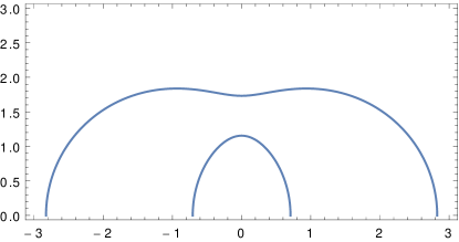
Figure 8. A hyperbola in the upper half-plane with foci at $i$ and $2i$, $c=\log(3/2)$, as drawn with Mathematica.

So this analysis shows that every two-focus hyperbola is also a focus-directrix hyperbola. The converse fails, however. Indeed, one can see from (3) that the focus-directrix hyperbola with $r=\varepsilon>1$ degenerates to the equation

$$(r^{2}+1)x^{2}+(r^{2}-1)y^{2}=\frac{r^{4}-1}{2},$$

which, surprisingly, is an ellipse in Cartesian coordinates. This has only one $y$-intercept in the upper half-plane, at the point $i\sqrt{\frac{r^{2}+1}{2}}$. So this “hyperbola” has only one vertex, the other vertex having gone to $+\infty i$, and this cannot be written as a two-focus hyperbola. ∎

References

- [1] Lars V. Ahlfors, Complex analysis, third ed., McGraw-Hill Book Co., New York, 1978, An introduction to the theory of analytic functions of one complex variable, International Series in Pure and Applied Mathematics. MR 510197 (80c:30001)
- [2] Friedrich Bachmann, Aufbau der Geometrie aus dem Spiegelungsbegriff, Springer-Verlag, Berlin-New York, 1973, Zweite ergänzte Auflage, Die Grundlehren der mathematischen Wissenschaften, Band 96. MR 0346643 (49 #11368)
- [3] H. S. M. Coxeter, Non-Euclidean geometry, sixth ed., MAA Spectrum, Mathematical Association of America, Washington, DC, 1998, first edition published 1942. MR 1628013 (99c:51002)
- [4] Géza Csima and Jenő Szirmai, Isoptic curves of conic sections in constant curvature geometries, Math. Commun. 19 (2014), no. 2, 277–290. MR 3274526
- [5] by same author, Isoptic curves of generalized conic sections in the hyperbolic plane, arXiv:1504.06450, 2015.
- [6] Kuno Fladt, Die allgemeine Kegelschnittsgleichung in der ebenen hyperbolischen Geometrie. II, J. Reine Angew. Math. 199 (1958), 203–207. MR 0095442 (20 #1944)
- [7] by same author, Elementare Bestimmung der Kegelschnitte in der hyperbolischen Geometrie, Acta Math. Acad. Sci. Hungar. 15 (1964), 247–257. MR 0171205 (30 #1436)
- [8] E. Molnár, Kegelschnitte auf der metrischen Ebene, Acta Math. Acad. Sci. Hungar. 31 (1978), no. 3-4, 317–343. MR 487028 (81e:51006)
- [9] William E. Story, On Non-Euclidean Properties of Conics, Amer. J. Math. 5 (1882), no. 1-4, 358–381. MR 1505334