Möbius Invariants of Shapes and Images

Möbius Invariants of Shapes and Images

Stephen MARSLAND ^† and Robert I. MCLACHLAN ^‡

S. Marsland and R.I. McLachlan

^† School of Engineering and Advanced Technology, Massey University,
^† Palmerston North, New Zealand s.r.marsland@massey.ac.nz http://www.stephenmonika.net

^‡ Institute of Fundamental Sciences, Massey University, Palmerston North, New Zealand r.mclachlan@massey.ac.nz http://www.massey.ac.nz/~rmclachl/

Received April 01, 2016, in final form August 08, 2016; Published online August 11, 2016

Identifying when different images are of the same object despite changes caused by imaging technologies, or processes such as growth, has many applications in fields such as computer vision and biological image analysis. One approach to this problem is to identify the group of possible transformations of the object and to find invariants to the action of that group, meaning that the object has the same values of the invariants despite the action of the group. In this paper we study the invariants of planar shapes and images under the Möbius group $\mathrm{PSL}(2,\mathbb{C})$, which arises in the conformal camera model of vision and may also correspond to neurological aspects of vision, such as grouping of lines and circles. We survey properties of invariants that are important in applications, and the known Möbius invariants, and then develop an algorithm by which shapes can be recognised that is Möbius- and reparametrization-invariant, numerically stable, and robust to noise. We demonstrate the efficacy of this new invariant approach on sets of curves, and then develop a Möbius-invariant signature of grey-scale images.

invariant; invariant signature; Möbius group; shape; image

68T45; 68U10

1 Introduction

Lie group methods play a fundamental role in many aspects of computer vision and image processing, including object recognition, pattern matching, feature detection, tracking, shape analysis, tomography, and geometric smoothing. We consider the setting in which a Lie group $G$ acts on a space $M$ of objects such as points, curves, or images, and convenient methods of working in $M/G$ are sought. One such method is based on the theory of invariants, i.e., on the theory of $G$-invariant functions on $M$, which has been extensively developed from mathematical, computer science, and engineering points of view.

When $M$ is a set of planar objects the most-studied groups are the Euclidean, affine, similarity, and projective groups. In this paper we make a first study of invariants of planar objects under the Möbius group $\mathrm{PSL}(2,\mathbb{C})$, which acts on the Riemann sphere $\overline{\mathbb{C}}=\mathbb{C}\cup\infty$ by

$$\phi\colon\ \overline{\mathbb{C}}\to\overline{\mathbb{C}},\qquad\phi(z)=\frac{az+b}{cz+d},\qquad a,b,c,d\in\mathbb{C},\qquad ad-bc\neq 0.$$

We work principally in the school of invariant signatures, developed by (amongst others) Olver and Shakiban [4, 9, 18, 30, 35, 36], and widely used for Euclidean object recognition (see, e.g., [2]).

$\mathrm{PSL}(2,\mathbb{C})$ is a 6-dimensional real Lie group. It forms the identity component of the inversive group, which is the group generated by the Möbius transformations and a reflection. In addition to its importance on fundamental grounds – it is one of the very few classes of Lie groups that act on the plane, it crops up in numerous branches of geometry and analysis, it is the smallest nonlinear planar group that contains the direct similarities, and it is the set of biholomorphic maps of the Riemann sphere – it also has direct applications in image processing since it arises in the conformal camera model of vision, in which scenes are projected radially onto a sphere [20, 39, 40]. It may also correspond to neurological aspects of vision, such as grouping of lines and circles (which are equivalent under Möbius transformations) [41].

From an applications point of view, different objects may be related by Möbius transformations, as is explored by Petukhov [34] for biological objects in fascinating detail in the context of Klein’s Erlangen program, giving examples of many body parts that are loxodromic to high accuracy (loxodromes have constant Möbius curvature and play the role in Möbius geometry that circles do in Euclidean geometry), that change shape by Möbius and other Lie group actions, and that grow via Möbius transformations (including 2D representations of the human skull). Other examples of 1-dimensional growth patterns, such as antenatal and postnatal human growth, appear to be well modelled by 1-dimensional linear-fractional transformations $x\mapsto(ax+b)/(cx+d)$. Discussing this work, Milnor [25] argued that “The geometrically simplest way to change the relative size of different body parts would be by a conformal transformation. It seems plausible that this simplest solution will often be the most efficient, so that natural selection tend to choose it”. (Milnor was thinking of 3D conformal transformations, whose restriction to 2D is the Möbius transformations.)

In this paper we present an integral invariant for the 2D Möbius group that is reparameterization independent, and demonstrate its use to identify curves that are related by Möbius transformations. We then consider the case of images, and describe an invariant signature by which Möbius transformed images can be recognised. We begin in Section 2 by discussing the desirable properties of invariants for object classification, and introduce the property of bounded distortion, which subsumes most of the requirements identified in the literature. This is followed by an overview of the methods that have been used to give object classification invariants for curves and images (most often with respect to the Euclidean, similarity, and affine groups).

In Section 3 we present the classical Möbius invariants and discuss their utility with respect to the properties identified in Section 2, before using a numerical example based on an ellipse to demonstrate the difference between them. This is followed by the introduction of the invariant that we have identified as the best behaved for curves with respect to the requirements previously discussed. In order to demonstrate its utility, we present an experiment where a set of smooth Jordan curves are created, and then the invariant distance is computed, and compared with direct registration of each pair of curves in the Möbius group using the $H^{1}$ similarity metric. The results show that the invariant is well-behaved with respect to noise, and can be used to separate all but the most similar shapes.

In Section 4 we move on to images and demonstrate the use of a 3D Möbius signature that is very sensitive and relatively cheap to compute, while still being more robust than the analogous signature for curves. As far as we know, such differential invariant signatures (in the sense of Olver [30]) for images have not been considered previously.

2 Invariants of shapes and images

2.1 Computational requirements of invariants for object classification

The mathematical definition of an invariant, namely, a $G$-invariant function on $M$, is not sufficiently strong for many computational applications. For example, object classification via invariants involves comparing the values of the invariant on different $G$-orbits, and the definition says nothing about this. Recognising this, Ghorbel [14] has given the following partial list of qualities needed for object recognition:

• fast computation;

• good numerical approximation;

• powerful discrimination (if two objects are far apart modulo $G$, their invariants should be far apart);

• completeness (two objects should have the same invariants iff they are the same modulo $G$);

• provide a $G$-invariant distance on $M$; and

• stability (if two objects have nearby invariants, they should be nearby modulo $G$).

Calabi et al. [9] include in (ii) the requirement that the numerical approximation itself should be $G$-invariant, while Abu-Mostafa et al. [1] add the further desirable qualities of:

• robustness (if two objects are nearby modulo $G$, especially when one is a noisy version of the other, their invariants should be nearby);

• lack of redundancy (i.e., all invariants are independent); and

• lack of suppression (in which the invariants are insensitive to some features of the objects).

Manay [21] includes, in addition:

• locality (which allows matching subparts and matching under occlusion).

To this already rather demanding list we add one more, that the set of invariants should be:

• small.

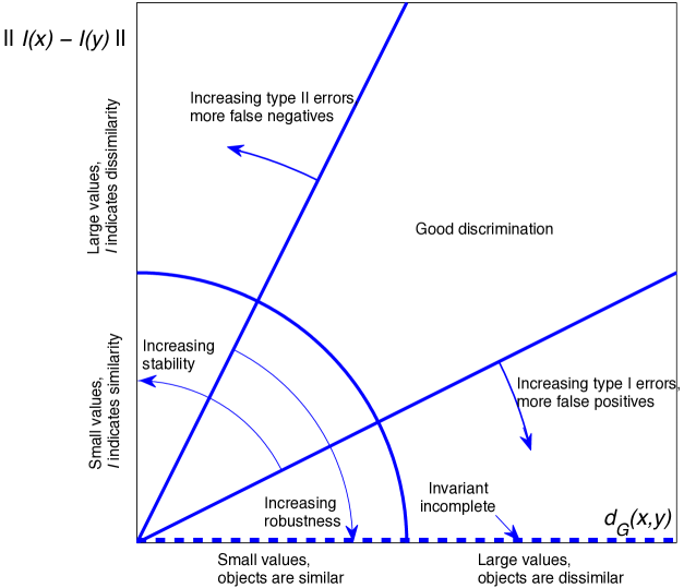
Figure 1: Sketch of the approximate relationships between $d_{G}(x,y)$, which measures the distance between two objects $x$ and $y$ modulo a symmetry group $G$, and $\|I(x)-I(y)\|$, which measures the distance between their invariants, illustrating the role of the desired properties of completeness, robustness, stability, and discrimination. In object recognition, ‘good discrimination’ is sometimes taken to mean the avoidance of type I errors (relative to the null hypothesis that two objects are in the same group orbit, so that in a type I error dissimilar objects are classified as similar), the avoidance of type II errors (similar objects being classified as dissimilar), or is not specified; we take it to mean that both type I and type II errors are avoided.

The motivation for this last is purely a parsimony argument; it is easy to produce large sets of invariants without adding much utility, and smaller sets of easily computable invariants are to be preferred. This is particularly the case since some of these criteria are in conflict, so there will usually not be one invariant that is preferred for all applications; instead, the best choice will depend on the dataset and the particular application. Others are closely related, especially discrimination, distance, stability, robustness, and suppression; these all depend on which features of the objects are deemed to be signal and which are deemed to be noise.

These criteria can be unified and quantified in the following way: suppose that a distance on objects has been chosen that measures the features that we are interested in (the signal), and that is small for differences that we are not interested in (the noise). This distance induces a distance on objects modulo $G$ by (where $\|\cdot\|_{d}$ is some appropriately chosen norm):

$$d_{G}(x,y):=\max\big{(}\inf_{g\in G}\|g\cdot x-y\|_{d},\,\inf_{g\in G}\|g\cdot y-x\|_{d}\big{)}.$$

(In principle one can compute $d_{G}(x,y)$ by optimizing over $G$, and indeed this is done in many applications. However, optimization is relatively difficult and unreliable, and becomes impractical on large sets of objects; this is the step that invariants are intended to avoid.) Suppose that a norm on invariants $I\colon M\to\mathbb{R}^{k}$ has been chosen. Then we can express the criteria as follows:

• discrimination: $d_{G}(x,y)\gg\varepsilon\Leftrightarrow\|I(x)-I(y)\|\gg\varepsilon$,

• completeness: $\|I(x)-I(y)\|=0\Rightarrow d_{G}(x,y)=0$,

• stability: $\|I(x)-I(y)\|\lesssim\varepsilon\Rightarrow d_{G}(x,y)\lesssim\varepsilon$,

• robustness: $d_{G}(x,y)\lesssim\varepsilon\Rightarrow\|I(x)-I(y)\|\lesssim\varepsilon$.

These may be subsumed and strengthened by the property of bounded distortion: an invariant has bounded distortion with respect to $d_{G}$ if there exist positive constants $c_{1}$, $c_{2}$ such that for all $x,y\in M$ we have

$$c_{1}d_{G}(x,y)\leq\|I(x)-I(y)\|\leq c_{2}d_{G}(x,y).$$ (2.1)

Suppose the invariant is to be used to test the hypothesis that two objects are the same modulo symmetry group $G$. The situation is illustrated in Fig. 1, which plots the distance between the invariants of two objects against the distance between the objects modulo $G$. The smaller the value of $c_{2}$, the more robust the invariant is, and the fewer false positives will be reported. The larger the value of $c_{1}$, the more stable the invariant is, the better its discrimination, and the fewer false negatives will be reported. If (2.1) holds only with $c_{1}=0$, the invariant is neither stable nor complete; if there is no $c_{2}$ such that (2.1) holds, the invariant is not robust. In addition, in some applications one may be more interested in some parts of the space shown in Fig. 1 than others: for example, in discriminating very similar or very dissimilar objects.

In practice, bounded distortion may not be possible. Even completeness, the centrepiece of the mathematical theory of invariants, can be very demanding. It turns out that many invariants that are roughly described as ‘complete’ are not fully complete, that is, they do not distinguish all group orbits, but only distinguish almost all group orbits. For example, Ghorbel’s Euclidean invariants of grey-level images [14] only distinguish images in which two particular Fourier coefficients are non-zero. Thus, it will be stable only on images in which these two Fourier coefficients are bounded away from zero. The most commonly-used Euclidean signature of curves, $(\kappa,\kappa_{s})$, is complete only on nondegenerate curves [17]. The fundamental issue is that even for very simple group actions, the space of orbits can be very complicated topologically, and thus very difficult (or even impossible) to coordinatize via invariants. We illustrate these ideas via an example:

Example 2.1.

Consider $n$ points $z_{1},\dots,z_{n}$ in the complex plane. Let $G=S^{1}$ act by rotating the points, i.e., $e^{i\theta}\cdot(z_{1},\dots,z_{n})=(e^{i\theta}z_{1},\dots,e^{i\theta}z_{n})$. Then $\{\bar{z}_{i}z_{j}\colon 1\leq i\leq j\leq n\}$ forms a complete set of invariants. It is very large (there are $n^{2}$ real components) compared to the dimension $2n-1$ of the space, $\mathbb{C}^{n}/S^{1}$, in which we are trying to work. However, if any one real component of the set is omitted, the resulting set is not complete. For example, if $|z_{1}|^{2}$ is omitted, then the points $(1,0,\dots,0)$ and $(2,0,\dots,0)$ have the same invariants, but do not lie on the same orbit. This is the situation considered in the problem of phase retrieval [6]. By choosing combinations of $\{\bar{z}_{i}z_{j}\}$ it is possible to create smaller sets of complete invariants, but the computational complexity of calculating the description of the $n$ points is still $\mathcal{O}(n^{2})$ [6].

In cases where one settles for an incomplete set of invariants, or a set that is not of bounded distortion – so that the worst-case behaviour of the invariants is arbitrarily poor – it can make sense instead to study the average-case behaviour of the invariants over some distribution of the objects. This is analogous to the role that ill-posed and ill-conditioned problems play in numerical linear algebra, although in that case the ill-conditioning is intrinsic rather than imposed by considerations of computational complexity. Indeed, one can sometimes very usefully describe objects based on an extremely small number of invariants, for example, describing planar curves by their length and enclosed area, or by the first few Fourier moments of their curvature. What is wanted is to optimize the behaviour of the invariants, over some distribution of the objects, with respect to their time and/or space complexity. However, we know of no genuine cases in which such a program has been carried out.

2.2 Invariants of curves

There is a large literature concerning invariants to the Euclidean and similarity groups for both curves and images. The purpose of this section is to provide an overview of the dominant themes within that work that are relevant to our goal of identifying invariants for the Möbius group that satisfy at least some of the criteria listed in the previous section.

We define a (closed) shape as the image of a function $\phi\colon S^{1}\to\mathbb{R}^{2}$. For different restrictions on $\phi$ this defines different spaces: if $\phi$ is a continuous injective mapping then this defines simple closed curves, while if $\phi$ is differentiable and $\phi^{\prime}(t)\neq 0$ for all $t$ this defines the ‘shape space’ $\operatorname{Imm}(S^{1},\mathbb{R}^{2})/\operatorname{Dif\/f}(S^{1})$ [26], while if $\phi$ is an immersion and $\phi(S^{1})$ is diffeomorphic to $S^{1}$, we obtain the shape space $\operatorname{Emb}(S^{1},\mathbb{R}^{2})/\operatorname{Dif\/f}(S^{1})$ (roughly, the curve has no self-intersections). There are also smooth ($C^{\infty}$) versions of these, piecewise smooth versions, shapes of bounded variation, and so on. The geometry of these shape spaces is now studied intensively in its own right [23, 24] as well as as a setting for computer vision; see [8] for a recent review.

The quotient by $\operatorname{Dif\/f}(S^{1})$ in the shape spaces has the effect of factoring out the dependence on the parameterization. Various methods have been used to achieve this, including:

1. Using a standard parameterization, such as Euclidean arclength. This leaves a dependence on the choice of starting point, i.e., the subgroup of $\operatorname{Dif\/f}(S^{1})$ consisting of translations is not removed.

2. Moment invariants, $\int_{0}^{L}f(\phi(s))\,\mathrm{d}s$, where $L$ is the length of the curve, $s$ is Euclidean arclength and $f$ ranges over a set of basis functions, such as monomials or Fourier modes [1].

3. Currents $\int_{S^{1}}\phi^{*}\alpha$, where $\alpha$ ranges over a set of basis 1-forms on $\mathbb{R}^{2}$, such as monomials times $\mathrm{d}x$ and monomials times $\mathrm{d}y$ [15].

The next step is to consider a Lie group $G$ acting on $\mathbb{R}^{2}$ that induces an action on the shape space. Here, many methods and types of invariants have been investigated (see, e.g., [42]).

The moving frame method

is a general approach to constructing invariants. Objects are put into a reference configuration and their resulting coordinates are then invariant. The moving frame or reference configuration method was developed as a way of finding differential invariants and variants of them (see [31] for an overview). A simple application of the method is the situation considered in Example 2.1, of $n$ points in the plane under rotations. Consider configurations with $z_{1}\neq 0$, $|\arg z_{1}|<\pi$. Rotate the configuration so that $z_{1}$ lies on the positive real axis. The coordinates of the resulting reference configuration, $\bar{z}_{1}z_{j}/|z_{1}|^{2}$, are invariant. In this case, the invariants are well behaved as $|\arg z_{1}|\to\pi$, but not as $z_{1}\to 0$.

Joint invariants

are functions of several points; for example, pairwise distances for a complete set of joint invariants for the action of the Euclidean group on sets of points in the plane.

Differential invariants

are functions of the derivatives of a curve at a point. There exist algorithms to generate all differential invariants [31]. For the action of the Euclidean group on planar curves, the Euclidean curvature $\kappa=\phi^{\prime}\times\phi^{\prime\prime}/\|\phi^{\prime}\|^{3}$ is $E(n)$ invariant (and parameterization invariant), and its derivatives $d^{n}\kappa/ds^{n}$ with respect to arclength form a complete set of differential invariants.

Semi-differential invariants

(also known as joint differential invariants [29]) of a curve are functions of several points and derivatives.

Integral invariants

are formed from the moments or the partial moments $\int_{s_{0}}^{s}f(\phi(t))\,\mathrm{d}t$. With some care they can be made parameterization- and basepoint-independent [11, 21]. Initially, these invariants appear to have some advantages, being relatively robust and often including some locality. However, they are not always applicable; for example [21], which used regional integral invariants, still requires a point correspondence optimization in order to get a distance between shapes. In addition, groups such as the projective group do not act on any finite subset of the moments [42]. Astrom [5] shows that there are no stable projective invariants for closed planar curves. While local integral invariants are promising, as reported by [16], there may be analytic difficulties in deriving them.

Another example of the moving frame method, which is common in image processing and shape analysis, is centre of mass reduction. The centre of mass of a shape may be moved to the origin in order to remove the translations. This may be calculated by, for example, $\int_{\phi(S^{1})}(x^{2}/2,xy)\mathrm{d}y=\iint_{\mathrm{int}\phi(S^{1})}(x,y)\mathrm{d}x\mathrm{d}y$. However, the shapes $x=a+\sin t$, $y=0$ have centre of mass equal to 0 for all values of $a$, even though they are related by translations. Thus, this method would not be robust on any dataset that contained shapes approaching such degenerate shapes. For rotations, the reference configuration method will not be robust if there are objects close to having a discrete rotational symmetry. The underlying problem with the reference configuration approach is that it is attempting to use a set of invariants equal to the dimension of the desired quotient space $M/G$. This space is almost always non-Euclidean, so such a set can only be found on some subset of $M/G$ of Euclidean topology. The set is then robust only on datasets that are bounded away from the boundary of this subset.

Calabi et al. [9] propose the use of differential invariant signatures for shape analysis, and further argue that these should be approximated in a group-invariant way. For example, for the Euclidean group, the signature is the shape $(\kappa,\kappa_{s})$ regarded as a subset of $\mathbb{R}^{2}$. The claimed advantages of the approach are that the signature determines the shape; that it does not depend on the choice of initial point on the curve or on parameterization by arclength, and that its $G$-invariance makes it robust; and that it is based on a general procedure for arbitrary objects and groups. See [2, 4, 9, 18, 30, 35, 36] for further developments and applications of the invariant signature.

Although the signature at first sight appears to be complete (e.g., Theorem 5.2 in [9]), a more detailed treatment (e.g., [17, 28]) highlights the fact that it is not complete on shapes that contain singular parts – straight and circular segments in the Euclidean case. For these parts, the signature reduces to a point. Thus, for shapes that have nearly straight or nearly circular segments, the signature cannot be robust. In addition, while the signature does not depend on the starting point or the parameterization, it takes values in a very complicated set, namely, the planar shapes. To compare the invariants of two shapes requires comparing two shapes. Essentially, the parameterization-dependence has only been deferred to a later stage of the analysis (unless one is content to compare shapes visually). One approach to this is to weight the signature, see [32] for more details.

The claim in [9] that the method’s $G$-invariance makes it robust should be assessed through further analysis and experiment. It would appear to be most relevant for datasets in which the errors due to the presentations of the shapes are comparable to those resulting from the errors in the shapes themselves (i.e., noise) and from the distribution of the objects in a classification problem. Their final point, that the method is extremely general, is a powerful one. Calabi [9] carry out the procedure for the Euclidean and for the 2D affine group. However in Section 6.7 they report that “the interpolation equations in general are transcendentally nonlinear and do not admit a readily explicit solution”, indicating that the method may not succeed for all group actions.

It is also possible to represent the shape as a binary image and apply image-based invariants (which are described next). This has the advantage of working directly in the space $\mathbb{R}^{2}$ on which the group acts, and avoiding all questions of parameterization, etc., but it does sacrifice a lot of information about the shape. A related approach, which is popular in PDE-based method for curves, is to represent the shape as the level set of a smooth function $\phi\colon\mathbb{R}^{2}\to\mathbb{R}$. This is also parameterization-independent, and retains smoothness, but we have never seen it used in for constructing invariants.

2.3 Invariants of images

Most studies of image invariants has been based on grey-level images $f\colon\Omega\to[0,1]$, where $\Omega\subset\mathbb{R}^{2}$. The methods are primarily based on moments [1] or Fourier transforms [14, 19] of the images, and have been highly developed for the translation, Euclidean, and similarity groups, where the linearity of the action and the special structure of these Lie groups means that the approach is particularly fast and robust. Attempts have been made to extend the method of Fourier invariants to other groups. There is an harmonic analysis for many non-Abelian Lie groups, including, in fact, the Möbius group [37], as well as a general theory for compact non-commutative groups [13]. There are some applications of this theory to image processing [19, 41] and to other problems in computational science. Fridman [12] discusses a Fourier transform for the hyperbolic group, the 3-dimensional subgroup of the Möbius group that fixes the unit disc. However, the theory appears not to have been developed to the point where it can be used as effectively as the standard Fourier invariants. Therefore, in this paper, in Section 4, we develop a Möbius invariant of images, based on a differential invariant signature of the image.

3 Möbius invariants for curves

In this section we consider invariants of curves for the Möbius group, and derive one suitable for practical computation, demonstrating its application for a set of simple closed curves.

3.1 Known Möbius invariants

The most well-known invariant of the Möbius group is the cross-ratio, also known as the wurf, which is based on the ratio of the distances between a set of 4 points:

$$\mathrm{CR}(z_{1},z_{2},z_{3},z_{4}):=\frac{(z_{1}-z_{3})(z_{2}-z_{4})}{(z_{2}-z_{3})(z_{1}-z_{4})},$$

where the invariance means that $\mathrm{CR}(Tz_{1},Tz_{2},Tz_{3},Tz_{4})=\mathrm{CR}(z_{1},z_{2},z_{3},z_{4})$ for Möbius transformation $T$.

Since the Möbius group can send any triple of distinct points in $\overline{\mathbb{C}}$ into any other such triple, there are no joint invariants of 2 or 3 points; the orbits are the configurations consisting of 1, 2, and 3 distinct points. When $n>4$, the set of cross-ratios of any four of the points forms a complete invariant.

For large numbers of points, this set of all cross-ratios has cardinality $\mathcal{O}(n^{4})$ which is impractically large (although some may be eliminated using functional relations amongst the invariants, known as syzygies [29]). However, if the dataset of shapes or images is tagged with a small number of clearly-defined landmarks, then some subset of the set of cross-ratios may form a useful invariant. This is the method by which Petukhov [34] was able to identify linear-fractional, Möbius, and projective relationships in biological shapes. For untagged objects, automatic tagging may be possible using critical points (e.g., maxima and minima) of images, and their values; these are homomorphism- and hence Möbius-invariant, and can be identified, even in the presence of noise, by the method of persistent homology [10]. However, such invariants are clearly highly incomplete for shapes and images, and we do not study them further here.

In order to derive differential invariants for the Möbius group, the most useful starting point is the Schwarzian derivative

$$(Sz)(t)=\left(\frac{z^{\prime\prime}}{z^{\prime}}\right)^{\prime}-\frac{1}{2}\left(\frac{z^{\prime\prime}}{z^{\prime}}\right)^{2}=\frac{z^{\prime\prime\prime}}{z^{\prime}}-\frac{3}{2}\left(\frac{z^{\prime\prime}}{z^{\prime}}\right)^{2}.$$ (3.1)

By an abuse of notation, which is standard in the literature (see, for example, the very readable [3]), the same formula (3.1) is used in three different situations: when $z\colon\mathbb{R}\to\mathbb{R}$ (used in studying linear-fractional mappings in real projective geometry); when $z\colon\overline{\mathbb{C}}\to\overline{\mathbb{C}}$ (used in studying complex analytic mappings); and when $z\colon M\to\overline{\mathbb{C}}$, $M$ a real 1-dimensional manifold (used in studying the Möbius geometry of curves). We adopt the latter setting so that $z^{\prime}$ is the tangent to the curve. The Schwarzian derivative is then invariant under Möbius transformations $\phi$:

$$S(\phi\circ z)(t)=S(\phi)(t)$$

and under reparameterizations $\psi\colon M\to M$ transforms as

$$S(z\circ\psi)=(S(z)\circ\psi)\cdot(\psi^{\prime})^{2}+S(\psi),$$

where the last term is the real Schwarzian derivative. Therefore (where $\operatorname{Im}$ represents the imaginary part of a complex number)

$$\operatorname{Im}S(z\circ\psi)=(\operatorname{Im}S(z)\circ\psi)\cdot(\psi^{\prime})^{2}.$$

This can be used to construct a distinguished Möbius-invariant parameterization of the curve. Let $\tilde{z}(\lambda)=z(t)$ where $\lambda=\psi(t)$. The parameter $\lambda$ will be chosen so that $\operatorname{Im}S(\tilde{z})\equiv 1$. This gives

$$\operatorname{Im}S(z)=\operatorname{Im}S(\tilde{z}\circ\psi)=(\operatorname{Im}S(\tilde{z})\circ\psi)\cdot(\psi^{\prime})^{2}=(\psi^{\prime})^{2}.$$

The choice $\psi^{\prime}(t)=\sqrt{|\operatorname{Im}S(z)(t)|}$ achieves this while preserving the sense of the curve, while the choice $\psi^{\prime}(t)=-\sqrt{|\operatorname{Im}S(z)(t)|}$ achieves it while reversing the sense. Put another way, the parameter

$$\lambda=\int_{t_{0}}^{t}\sqrt{|\operatorname{Im}S(z)(t)|}$$

is invariant under Möbius transformations and almost invariant under sense-preserving reparameterizations of $t$, which act as translations in $\lambda$ (because of the freedom to choose $t_{0}$). Equivalently, the 1-form

$$\mathrm{d}\lambda=\sqrt{|\operatorname{Im}S(z)(t)|}\mathrm{d}t,$$

known as the Möbius or inversive arclength, is Möbius- and sense-preserving parameterization-invariant.

This is often stated in a form (originally due, according to Ahlfors [3], to Georg Pick) using the Euclidean curvature $\kappa$. If the curve is parameterized by Euclidean arclength $s$, then its tangent $\theta(s)=z^{\prime}(s)/\|z^{\prime}(s)\|$ and $\kappa(s)=\theta^{\prime}(s)$. Differentiating again leads to $\operatorname{Im}S(z)(s)=\kappa^{\prime}(s)$, or

$$\mathrm{d}\lambda=\sqrt{|\kappa^{\prime}(s)|}{\rm d}s.$$

The 1-form $\mathrm{d}\lambda$ provides a useful discrete invariant, the Möbius length $L$ of the curve

$$L=\int_{M}\mathrm{d}\lambda.$$

The real part of $S(\tilde{z})(\lambda)$ is now a parameterization-invariant Möbius invariant known as the inversive or Möbius curvature [33]

$$\kappa_{{\text{\tiny M\"{o}b}}}=\frac{4\kappa^{\prime}(\kappa^{\prime\prime\prime}-\kappa^{2}\kappa^{\prime})-5(\kappa^{\prime\prime})^{2}}{8(\kappa^{\prime})^{3}},$$

where ^′ denotes differentiation with respect to arclength $s$.

The set of all differential Möbius shape invariants is then $\mathrm{d}^{n}\kappa_{{\text{\tiny M\"{o}b}}}/d\lambda^{n}$, $n\geq 0$. Following Calabi et al. [9], two possible candidate invariants that could be used to recognize Möbius shapes are the function $\kappa_{\text{\tiny M\"{o}b}}(\lambda)$ modulo translations and the signature $(\kappa_{\text{\tiny M\"{o}b}},\mathrm{d}\kappa_{\text{\tiny M\"{o}b}}/\mathrm{d}\lambda)(S^{1})\subset\mathbb{R}^{2}$. These are complete on sections of shapes with no vertices (points where $\kappa^{\prime}(s)=0$). However, since $\kappa_{\text{\tiny M\"{o}b}}$ requires the 5th derivative of the curve (third derivative of the curvature), it is not robust in the presence of noise, and we do not explore it further.

There are also invariants based on forms of higher degree. We give just one example, the Möbius energy

$$-\frac{1}{2}\iint_{M\times M}\frac{\sin\theta_{u}\sin\theta_{v}}{|v-u|^{2}}\mathrm{d}u\,\mathrm{d}v,$$ (3.2)

introduced by O’Hara and Solanes [27], see also the related Kerzman–Stein distance [7]. Here $\mathrm{d}u$, $\mathrm{d}v$ are Euclidean arclength and $\theta_{u}$ (resp. $\theta_{v}$) is the angle between $v-u$ and $z^{\prime}(u)$ (resp. $v$). It represents a renormalization of the energy of particles on the curve, distributed evenly with respect to Euclidean arclength and interacting under an $r^{-4}$ potential. (The authors of [27] comment that “due to divergence problems, almost nothing is known about integral geometry [i.e., about invariant differential forms] under the Möbius group”.) The Möbius energy has one distinguishing feature compared to the other invariants: its definition depends only on the first derivative of the curve. The singularity at $u=v$ is removable, since the integrand obeys

$$\frac{\sin\theta_{u}\sin\theta_{v}}{|v-u|^{2}}=\frac{1}{4}\kappa(u)\kappa(v)+\mathcal{O}(|v-u|).$$

Thus, the energy is defined for $C^{2}$ curves, and even near the singularity it depends only on the curvature of the curve.

However, in numerical experiments we found the integrand of (3.2) difficult to evaluate accurately and invariantly, particularly near the diagonal, while the double integral generated little improvement in robustness. The most negative feature of the energy is its cost: its evaluation apparently requires considering all pairs of points on a discrete curve. There is another reason why invariant 2-forms are less useful than invariant 1-forms like $\mathrm{d}\lambda$: invariant $k$-forms distinguish coordinates on $M^{k}$ only up to $k$-form- (i.e., volume-) preserving maps. These are infinite-dimensional for $k>1$, but 1-dimensional for $k=1$: the coordinates are determined up to translations. For these reasons, we do not consider the energy, or related invariant 2-forms, any further.

Finally, Möbius transformations map circles to circles, and thus critical points of Euclidean curvature (the ‘vertices’ of the shape) are Möbius invariants. The four vertex theorem states that all smooth curves have at least four vertices. The number of vertices is a discrete Möbius invariant. Consequently, sections of shapes on which the Euclidean curvature is monotonic, and their Möbius lengths, are Möbius invariant.

3.2 Example: Evaluating the Möbius length of an ellipse

Having described a number of possible invariants, and ruled many of them out based on the criteria discussed in Section 2.1, we now provide a concrete example, illustrating and testing some of these constructions on the ellipse $z(t)=\cos 2\pi t+2{\rm i}\sin 2\pi t$, $0\leq t\leq 1$. The ellipse is discretized at $t_{i}=(i+1/4)h$, $i=0,\dots,n$, giving points $z_{i}=z(t_{i})$, and the Möbius arclength $\mathrm{d}\lambda$ is calculated in two ways:

• From the curvature method, in which the Euclidean curvature $\kappa$ is calculated in a Euclidean-invariant way by interpolating a circle through 3 adjacent points, and $\mathrm{d}\kappa/\mathrm{d}s$ by a finite difference, giving

  $$\mathrm{d}\lambda(t_{i+3/2})\approx|\kappa(z_{i+1},z_{i+2},z_{i+3})-\kappa(z_{i},z_{i+1},z_{i+2})|(|z_{i+2}-z_{i+1}|).$$ (3.3)

• From the cross-ratio method, using

  $$\mathrm{d}\lambda(t_{i+3/2})\approx\sqrt{6|\mathrm{Im}(\log(\mathrm{CR}(z_{i},z_{i+1},z_{i+2},z_{i+3})))|}.$$ (3.4)

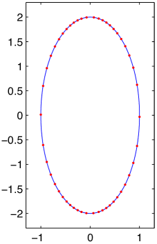
Figure 2: The ellipse used as a test case, showing 50 points equally spaced with respect to Möbius arclength.

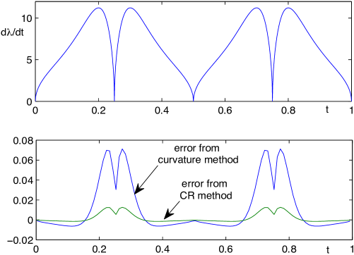
Figure 3: The Möbius arclength density, $\mathrm{d}\lambda/\mathrm{d}t$, for the ellipse, and its errors when calculated by the two approximations (3.3) and (3.4).

Away from vertices (points where $\mathrm{d}\lambda=0$), both of these are second-order finite difference approximations to the Möbius length $\int_{t_{i+1}}^{t_{i+2}}\mathrm{d}\lambda$ of the arc $z([t_{i+1},t_{i+2}])$, or, dividing by $h$, to its arclength density $\mathrm{d}\lambda/\mathrm{d}t$. This can be established by expanding the approximations in Taylor series. We test their accuracy as a function of the step size $h$. The total Möbius length of the curve is

$$L:=\int_{0}^{1}d\lambda=\int_{0}^{1}\frac{12\pi\sqrt{|\sin 4\pi t|}}{5+3\cos 4\pi t}\,\mathrm{d}t=6.86\quad(\mbox{to }2\mbox{ d.p.}).$$

The arclength density $\mathrm{d}\lambda/\mathrm{d}t$ is shown in Fig. 3, showing its 4 zeros at the vertices of the ellipse, where the ellipse is approximately circular, and its square-root singularities at the vertices. The Möbius length is approximated by the trapezoidal rule, i.e., by $L_{h}:=\sum\limits_{i=1}^{n}\mathrm{d}\lambda(t_{i+1/2})$. The error $L-L_{h}$ is expected to have dominant contributions of order $h^{3/2}$, due to the singularities at the vertices, and of order $h^{2}$, due to the finite differences used to approximate $\mathrm{d}\lambda$.

In this example, the cross-ratio approximation has errors approximately 0.176 times those of the curvature approximation (see Fig. 3). However, due to some cancellations in this particular example, the curvature approximation actually gives a slightly more accurate approximation to the Möbius length (see Fig. 4). The dominant sources of error can be eliminated by two steps of Richardson extrapolation, first to remove the $\mathcal{O}(h^{3/2})$ error, and then to remove the $\mathcal{O}(h^{2})$ error. This is highly successful and allows the calculation of the Möbius length with an error of less than $10^{-10}$, even though it is singular and involves a 3rd derivative.

Next, we subject the ellipse to a variety of Möbius transformations. The resulting shapes and errors are shown in Fig. 5. The errors increase markedly for the curvature method, which is not Möbius invariant, but are unchanged for the cross-ratio method, which is Möbius invariant. Thus, this experiment supports the argument of [9] that numerical approximations of invariants should themselves be invariant.

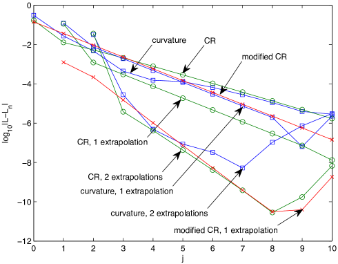
Figure 4: The error in the two approximations of the total Möbius length of the ellipse. Here there are $n:=25\cdot 2^{j}$ points on the ellipse.

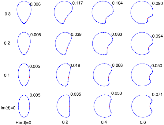
Figure 5: The ellipse subjected to 16 different Möbius transformations $z\mapsto\frac{z}{1+dz}$. 10 landmarks, equally spaced in $\lambda$, are shown. Next to each shape is given the error in its Möbius length as calculated by the curvature method. The error in the cross-ratio method is $0.005$ for all shapes, because it is Möbius invariant. (The other Möbius transformations are the Euclidean similarities, which are easy to visualize. Figures not to scale.)

3.3 The Möbius invariant $\boldsymbol{\mathrm{CR}(\lambda;z,\delta)}$

The method proposed in this paper for closed curves is to parameterize the curve by Möbius arclength, giving $z(\lambda)$, and to use as an invariant the cross-ratio of all sets of 4 points a distance $\delta$ apart. We call this the Shape Cross-Ratio, or SCR.

Definition 3.1.

Let $z\colon S^{1}\to\mathbb{C}$ be a smooth curve. Let $L$ be its Möbius length, and let $\tilde{z}\colon\mathbb{R}\to\mathbb{C}$ be an $L$-periodic function representing the curve parameterized by Möbius arclength. The shape cross-ratio of $z$ is the $L$-periodic function $\mathrm{SCR}\colon\mathbb{R}\to\overline{\mathbb{C}}$ defined by

$$\mathrm{SCR}(\lambda;z,\delta)=\mathrm{CR}(\tilde{z}(\lambda),\tilde{z}(\lambda+\delta),\tilde{z}(\lambda+2\delta),\tilde{z}(\lambda+3\delta)).$$

The shape cross-ratio signature of $z$ is the shape $\mathrm{SCR}(\mathbb{R};z,\delta)\subset\overline{\mathbb{C}}$.

The shape cross-ratio is invariant under the Möbius group, and sense-preserving reparameterizations of the curve act as translations in $\lambda$. (Reversals of the curve will be considered in Section 3.5.) The shape cross-ratio signature is invariant under the Möbius group and under reparameterizations of the curve.

For an $L$-periodic function $f\colon\mathbb{R}\to\mathbb{C}$ we will denote its Fourier coefficients by

$$\mathcal{F}(f)_{n}=\frac{1}{L}\int_{0}^{L}f(t)e^{-2\pi{\rm i}nt/L}\mathrm{d}t.$$

The translation $t\mapsto t+c$ acts on the Fourier coefficients as $\mathcal{F}(f)_{n}\mapsto e^{-2\pi{\rm i}cn/L}\mathcal{F}(f)_{n}$. The Fourier amplitudes $|\mathcal{F}(f)_{n}|^{2}$ are invariant under translations, and can be used to recognize functions up to translations, but are clearly not a complete invariant: for a function discretized at $N$ equally-spaced points, and using the DFT, the space of orbits has dimension $2N-1$ and we have only $N$ invariants. The bispectrum [19] $\mathcal{F}(f)_{m}\mathcal{F}(f)_{n}\mathcal{F}(f)_{-m-n}$ is better, being complete on functions all of whose Fourier coefficients are non-zero, but it is a very large set of invariants. Other invariants are $\mathcal{F}(\phi_{1}\circ f)_{n}\mathcal{F}(\phi_{2}\circ f)_{-n}$ for any functions $\phi_{1,2}$. Each such choice provides $2N$ invariants. The choice of $\phi_{1}$ and $\phi_{2}$ determines which aspects of $f$ are measured by the invariant. If necessary, several such pairs may be used.

Definition 3.2.

The Fourier cross-ratio of the shape $z$ is

$$\mathrm{FCR}(\cdot;z,\delta)\colon\ {\mathbb{Z}}\to\mathbb{C},\qquad\!\!\mathrm{FCR}(n;z,\delta)=\mathcal{F}(\phi_{1}\circ\mathrm{SCR}(\cdot;z,\delta))_{n}\mathcal{F}(\phi_{2}\circ\mathrm{SCR}(\cdot;z,\delta))_{-n},\!\!$$ (3.5)

where the Fourier transforms are based on the Möbius length $L$ of $z$.

In the numerical illustrations we use

$$\phi_{1}(w)=\frac{w}{\sqrt{1+|w|^{2}}},\qquad\phi_{2}(w)=\phi_{1}(w)^{2}$$ (3.6)

and the distance between the invariants of two shapes $z_{1}$ and $z_{2}$ given by

$$\|\mathrm{FCR}(\cdot;z_{1},\delta)-\mathrm{FCR}(\cdot;z_{2},\delta)\|_{2}.$$ (3.7)

The motivation here is that the cross-ratio becomes arbitrarily large when two different parts of the curve approach one another. If left untouched (i.e., if we use just $\phi_{1}(w)=w$), then these large spikes in $\mathrm{SCR}(\lambda;z,\delta)$ will dominate all other contributions to the shape measurement. By scaling them using (3.6), they will still contribute to the description of the shape, but in a way that is balanced with respect to other parts of the shape. $\phi_{1}$ and $\phi_{2}$ take values in the unit disk and $\phi_{2}$ is sensitive to the main range of features of shapes; only values of $\mathrm{SCR}$ near 0 are suppressed, and these are rare.

The invariant $\mathrm{SCR}(\lambda;z,\delta)$ is smooth on simple closed curves, and also on most curves with self-intersections (blow-up requires the close approach of two points Möbius distance $n\delta$ apart). It is locally complete, as given $z([a,a+3\delta])$, the invariant $\mathrm{SCR}(\lambda)$ determines $z$. We do not know if it is globally complete, i.e., if, given $\mathrm{SCR}(\lambda)$ which is the invariant of some shape, the shape can be determined up to Möbius transformations, because this requires solving a nonlinear functional boundary value problem. Subject to this restriction, the invariant $\mathrm{FCR}(n;z,\delta)$ is complete except on a residual set of shapes (those for which enough Fourier coefficients in (3.5) are zero).

We will first study the numerical approximation of $\mathrm{SCR}$ and then study its use in recognizing shapes modulo Möbius transformations.

The numerical experiments in Section 3.2 convinced us to approximate the Möbius arclength using the cross-ratio. However, when combined with piecewise linear interpolation to locate points on the curve the required distance $\delta$ apart, we found that the resulting values of $\mathrm{SCR}(\lambda;z,\delta)$ did not converge as $h\to 0$. This is due to accumulation of errors along the curve, which arise particularly at the vertices due to the singularities there. This prompted us to develop a more refined interpolation method that takes into account the singularities of $\mathrm{d}\lambda/\mathrm{d}t$ at the vertices. We call it the modified cross-ratio method:

1. Calculate the square of the Möbius arclength density at the centre of each cell, as

   $$\left(\frac{\mathrm{d}\lambda}{\mathrm{d}t}\right)^{2}_{i+3/2}=6\operatorname{Im}(\log(\mathrm{CR}(z_{i},z_{i+1},z_{i+2},z_{i+3}))).$$

   If the curve is smooth, this is a smooth function.

2. Let $f(t)$, $0\leq t<1$, be the piecewise linear interpolant of $\left(\frac{\mathrm{d}\lambda}{\mathrm{d}t}\right)^{2}_{i+3/2}$.

3. Calculate $\lambda(t)=\int_{0}^{t}\sqrt{|f(\tau)|}\,\mathrm{d}\tau$ and its inverse, $t(\lambda)$, used in locating the parameter values at which points a desired length apart are located, exactly (we omit the formulas).

4. The desired points $z(t(\lambda+n\delta))$ are calculated using linear interpolation from the known values $z(ih)$.

5. The cross-ratio is evaluated at $N$ points equally spaced in $\lambda$, giving $\mathrm{SCR}(iL/N;z,\delta)$ for $i=1,\dots,N$, and the Fourier invariant $\mathrm{FCR}$ evaluated using two FFTs.

The resulting cross-ratio is globally second-order accurate in $h$. Its accuracy could be increased for smooth curves using higher order interpolation, but the calculation of the inverse $t(\lambda)$ would be much more complicated and the method would be less robust.

The error in the length $L$ of the ellipse used in Section 3.2 as calculated by this method is shown in Fig. 4. It behaves extremely reliably over a wide range of scales of $h$; its error after one Richardson extrapolation is observed to be $\mathcal{O}(h^{4})$, which indicates that the singularities at the vertices have been completely removed.

The parameter $\delta$ is the length scale on which $\mathrm{SCR}(\lambda;z,\delta)$ describes the shape. However, if $\delta\to 0$ then $\mathrm{SCR}(\lambda;z,\delta)\to\kappa_{\text{\tiny M\"{o}b}}\pm\mathrm{i}$: the real part becomes extremely nonrobust and the imaginary part yields no information [33]. In the experiments in this paper we have used $\delta=L/8$. Choosing $L/\delta\in\mathbb{Z}$ seems to yield somewhat improved accuracy, as the same values of $z$ are used repeatedly.

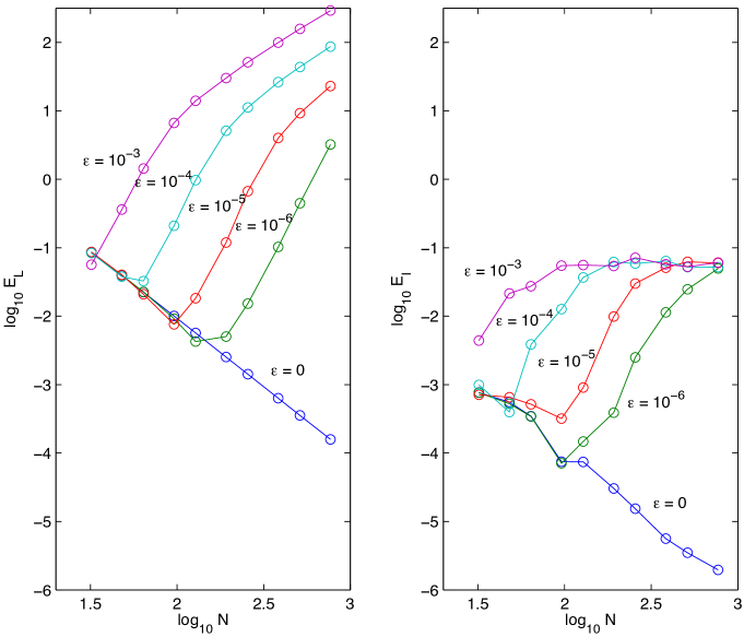
Figure 6: Average error in $L$ (left) and $\mathrm{FCR}$ (right) for the ellipse shown in Fig. 2 as a function of the number of points $N$ and noise level $\varepsilon$.

As the method relies on parameterization by Möbius arclength, it is unavoidably sensitive to noise in the data. We test its sensitivity for a noise model in which each point on the discrete curve is subject to normally distributed noise of standard deviation $\varepsilon$. The dependence of the error on $\epsilon$ and $N$ is shown for length and cross-ratio invariants in Fig. 6. Clearly, both are sensitive to relatively small amounts of noise. However, some positive features can also be seen:

• The errors in $L$ and $\mathrm{FCR}(n;z,\delta)$ are both $\mathcal{O}(h^{2})$ in the absence of noise.

• The errors in $\mathrm{FCR}(n;z,\delta)$ are much smaller than those in $L$ – their relative errors are about 8 times smaller. (For the ellipse, $L\approx 6.86$ and $\|\mathrm{SCR}(\cdot;z,\delta)\|_{2}\approx 0.65$.)

• The error in $\mathrm{FCR}(n;z,\delta)$ appears to saturate at about 13% as $\varepsilon$ increases and as $N$ increases.

Point (iii) is particularly striking. It appears to hold because (a) $\delta$ is chosen to be proportional to $L$, and thus when the noise is high, the chosen points stay roughly in their correct places; and (b) noise in the chosen points is averaged out by the Fourier transform, which remains dominated by its first few terms. This effect is illustrated in Fig. 7 in which a single noise realization is illustrated for value of $\varepsilon$ from 0 to $10^{-2}$. Even though $L$ is overestimated by a factor of 100, the signature cross-ratio $\mathrm{SCR}(\lambda;z,\delta)$ is still recognizable.

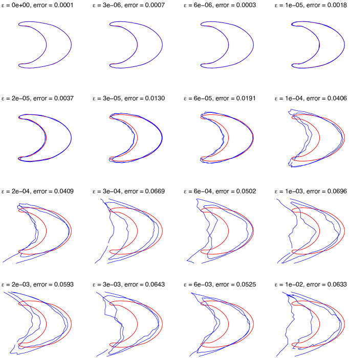
Figure 7: The cross-ratio signature $\mathrm{SCR}\colon S^{1}\to\mathbb{C}$ (blue), and the error in its Fourier invariant $\mathrm{FCR}$, is shown for the ellipse discretized with $N=128$ points and various levels of noise. The exact signature is shown in red.

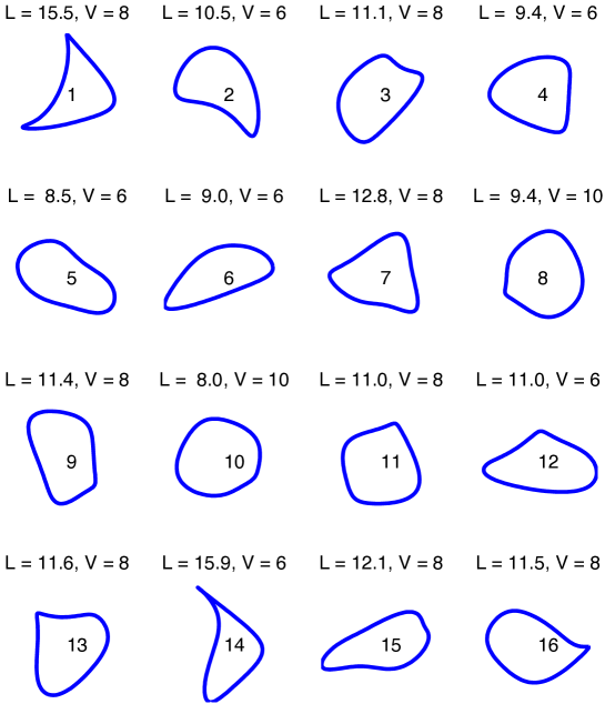
Figure 8: The set of 16 shapes used in the numerical experiments. The shapes are shown to scale with the shape number marking the origin, along with the shape’s Möbius length $L$ and number of vertices $V$.

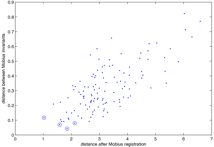
Figure 9: Scatter plot of distance between all 120 pairs of 16 shapes with respect to (i) the $H^{1}$ distance between the shapes, as defined in (3.8)–(3.10), and (ii) the distance between their Möbius invariants, defined in (3.5)–(3.7). The correlation coefficient is 0.85. The registration between the 4 pairs marked with circles is illustrated in Figs. 10–13.

3.4 Comparison with shape registration

We now compare the results of the Möbius invariant $\mathrm{FCR}(n;z,\delta)$ with direct registration of shapes. Given two shapes $z$ and $w$ we define the $G$-registration of $z$ onto $w$ as

$$r_{G}(z,w)=\min_{\varphi\in G\atop\psi\in\operatorname{Dif\/f}^{+}(S^{1})}\|\varphi\circ z\circ\psi-w\|.$$ (3.8)

Different choices of norm in (3.8) will give different registrations; we have used the $H^{1}$ norm

$$\|z\|_{H^{1}}^{2}=\int_{0}^{1}|z(t))|^{2}+\alpha|z^{\prime}(t))|^{2}\,\mathrm{d}t,$$ (3.9)

where the constant $\alpha$ was chosen as $0.1$, a value which made both contributions to the norm roughly equal. One of the peculiarities of the Möbius group is that $z$ may register very well onto $w$ while $w$ registers poorly onto $z$. This happens when $z$ has a distinguished feature which can be squashed, thus minimizing its contribution to $r_{G}(z,w)$. Therefore in our experiments we use the ‘distance’

$$d_{G}(z,w)=\max(r_{G}(z,w),r_{G}(w,z)).$$ (3.10)

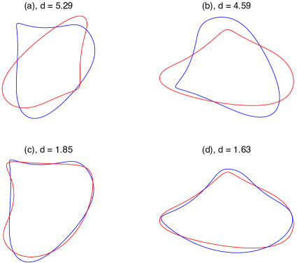
Figure 10: Registration of shapes 12 (blue) & 13 (red). This pair has the closest Möbius invariants (distance 0.0426, see (3.7)), is 9th closest after Möbius registration, and 96th closest after similarity registration. (a) Similarities act on blue shape; (b) Similarities act on red shape; (c) Möbius acts on blue shape; (d) Möbius acts on red shape. Here $d=r_{G}(x,y)$ where $x$ and $y$ are the two shapes, see equation (3.8).

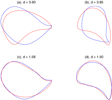
Figure 11: Registration of shapes 2 (blue) & 16 (red). This pair has the 2nd closest Möbius invariants (distance 0.0697), see (3.7)), is 3rd closest after Möbius registration, and 42rd closest after similarity registration. (a) Similarities act on blue shape; (b) Similarities act on red shape; (c) Möbius acts on blue shape; (d) Möbius acts on red shape. Here $d=r_{G}(x,y)$ where $x$ and $y$ are the two shapes, see equation (3.8).

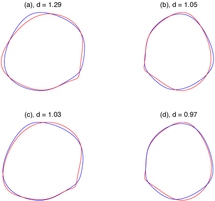
Figure 12: Registration of shapes 8 (blue) & 10 (red). This pair is closest after Möbius registration. It has the 11st closest Möbius invariants (distance 0.1165) and is the closest pair after similarity registration. (a) Similarities act on blue shape; (b) Similarities act on red shape; (c) Möbius acts on blue shape; (d) Möbius acts on red shape. Here $d=r_{G}(x,y)$ where $x$ and $y$ are the two shapes, see equation (3.8).

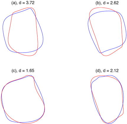
Figure 13: Registration of shapes 9 (blue) & 11 (red). This pair has the 3rd closest Möbius invariants (distance 0.0798), is 9th closest after Möbius registration, and 96th closest after similarity registration. (a) Similarities act on blue shape; (b) Similarities act on red shape; (c) Möbius acts on blue shape; (d) Möbius acts on red shape. Here $d=r_{G}(x,y)$ where $x$ and $y$ are the two shapes, see equation (3.8).

Note that this should not be regarded as any kind of ‘ground truth’ for the $G$-similarity of $z$ and $w$. It is not $G$-invariant. However, as we shall see, it does correspond remarkably well to the Möbius invariants described earlier.

To calculate $d_{G}(z,w)$ numerically, we discretize $\operatorname{Dif\/f}^{+}(S^{1})$ by piecewise linear increasing functions with 16 control points and perform the optimization using Matlab’s lsqnonlin, with initial guesses for $\varphi$ chosen to be each of 4 rotations and 3 scale factors for $\varphi$, and initial $\psi$ chosen to be the identity.

We generated 16 random shapes from a 14-dimensional distribution that favours smooth Jordan curves of similar sizes (where $U(0,2\pi)$ denotes uniform random numbers in the range $0$ to $2\pi$):

$$z(t)=\sum_{n=-4}^{4}a_{n}\mathrm{e}^{2\pi\mathrm{i}nt},\qquad\operatorname{Re}(a_{n}),\,\operatorname{Im}(a_{n})\in N\big{(}0,1/\big{(}1+|n|^{3}\big{)}\big{)},\qquad n\neq\pm 1,$$

$$\arg a_{1}\in U(0,2\pi),\qquad|a_{1}|=1,\qquad a_{-1}/a_{1}\in U(0,0.6).$$

The shapes are shown in Fig. 8. They are all simple closed curves, which we take to be positively oriented. The 120 pairs of distinct shapes are registered in both directions, and the scatter plot between this distance and the 2-norm of the distance between their invariants is shown in Fig. 9. The correlation (0.85) is extremely striking, and suggests that this pair of measures may be related by bounded distortion (2.1), implying that they meet many of the requirements that we identified in Section 2.1; they are also quick to compute and provide a good numerical approximation.

Some examples of the registrations in the similarity and Möbius groups are shown for four close pairs in Figs. 10–13. Including the invariants $L$ and $V$ in the list of invariants did not improve the correlation. Note that the errors in $\|\mathrm{FCR}(\cdot;z,\delta)\|$ observed in Fig. 4 are small enough to allow the separation of all but the closest pairs of shapes, regardless of the level of noise $\varepsilon$.

3.5 Reversals and reflections

Orientation reversals and reflections are examples of actions of discrete groups and can, in theory, be handled by any of the approaches in Section 2.2. First, consider the sense-reversing reparameterizations, $z(t)\mapsto z(-t)$. These map the SCR invariant as $\mathrm{SCR}(\lambda;z,\delta)\mapsto\mathrm{SCR}(-\lambda;z,\delta)$ and hence $\mathrm{FCR}(n)\mapsto\mathrm{FCR}(-n)$. It is convenient to pass to the equivalent invariants:

$$x_{n}=\begin{cases}\mathrm{FCR}(n)-\mathrm{FCR}(-n),&n>0,\\ \mathrm{FCR}(n)+\mathrm{FCR}(-n),&n\leq 0,\end{cases}$$

for which $x_{n}$ is invariant for $n\leq 0$ and $x_{n}\mapsto-x_{-n}$ for $n>0$. Suppose that we wish to identity curves with their reversals, that is, to work with unoriented shapes. Some options are the following:

1. The moving frame method: the shapes are put into a reference orientation first. This is only possible if the problem domain is restricted suitably; in this case, for example, to simple closed curves, which can be taken to be positively oriented. This is the approach that we have taken in Sections 3.3 and 3.4. If the problem domain includes non-simple curves this approach may not be possible. For example, in the space of plane curves with the topology of a figure 8, each such shape can be continuously deformed into its reversal; thus we cannot assign them orientations, since they vary continuously with the shape.

2. Finding a complete set of invariants: this is $x_{n}$ for $n\leq 0$ and $x_{i}x_{j}$ for $i,j>0$. Again we see that the quotient by a relatively simple group action is expensive to describe completely using invariants.

3. Use an incomplete set of invariants that is “good enough”: here, using $x_{n}$ for $n\leq 0$ and $x_{n}x_{n+1}$ for $n>0$ is a possibility. This creates a complicated effect on the metric used to compare invariants.

4. As the group action is of a standard type, one can work in unreduced coordinates ($x_{n}$) together with a natural metric induced by the quotient, such as some function of $\|x\|-\|y\|$ and the Fubini–Study metric on projective space, $\cos^{-1}(|\bar{x}^{T}y|/\|x\|\|y\|)$.

5. Finally, and most easily in this case, for finite groups one can represent points in the quotient as entire group orbits. A suitable metric is then

   $$d(x,y)=\min_{g\in G}\|x-g\cdot y\|,$$

   where $G$ is the group. Although this is impractical for large finite groups, here $G$ is $\mathbb{Z}_{2}$.

Similar considerations apply to recognizing shapes modulo the full inversive group, generated by the Möbius group together with a reflection, say $z\mapsto\bar{z}$. The reflection maps $\mathrm{FCR}(n)\mapsto\overline{\mathrm{FCR}(n)}$ and hence is an action of the same type as reversal (a sign change in some components). The reflection symmetry of the ellipse in Fig. 2, for example, can be detected by the reflection symmetry of the cross-ratio signature $\mathrm{SCR}(\lambda)$ in Fig. 7. (Its second discrete symmetry, a rotation by $\pi$, is manifested in Fig. 7 by the signature curve retracting itself twice.)

The invariants developed here are for closed shapes. They can be adapted for other types of shapes (for example, shapes with the topology of two disjoint circles), but as the topology gets more complicated (for example, shapes consisting of many curve segments) the problem becomes significantly more difficult.

4 Möbius invariants of images

Let $f\colon\overline{\mathbb{C}}\to[0,1]$ be a smooth grey-scale image. Diffeomorphisms act on images by $\varphi\cdot f:=f\circ\varphi^{-1}$. It is easy, in principle, to adapt the Möbius shape invariant $\mathrm{SCR}$ to images by computing level sets of $f$, each of which is an invariant shape for which $\mathrm{SCR}$ can be calculated. In addition, if $\varphi$ is conformal, the orthogonal trajectories of the level sets, i.e., the shapes tangent to $\nabla f$, are also invariant shapes. In the neighbourhood of a simple closed level set, coordinates $(\lambda,\mu)$ can be introduced, where $\lambda$ is Möbius arclength along the level set and $\mu$ is Möbius arclength along the orthogonal trajectories. The quantity

$$\mathrm{CR}(z(\lambda,\mu),z(\lambda,\mu+\delta),z(\lambda+\delta,\mu+\delta),z(\lambda+\delta,\mu)),$$ (4.1)

calculated from the cross-ratio of 4 points in a square, is then invariant under the Möbius group, and reparameterizations of the level set act as translations in $\lambda$.

In practice, however, the domain of this invariant is quite restricted. The topology of level sets is typically very complicated and the domain of $f$ may be restricted, so that level sets can stop at the edge of the image. Restricting to level sets of grey-scales near the maximum and minimum of $f$ helps, but this is a severe restriction. Instead, we shall show that the extra information provided by an image, as opposed to that provided by a shape, determines a differential invariant signature using only 3rd derivatives, compared to the 5th derivatives needed for differential invariants of shapes. Because of this, we do not develop the cross-ratio invariant (4.1) any further here.

Proposition 4.1.

Let $f\colon\overline{\mathbb{C}}\to\mathbb{R}$ be a smooth grey-scale image. Let $R\subset\overline{\mathbb{C}}$ be the regular points of $f$. Identify $x_{1}+{\rm i}x_{2}\in\mathbb{C}$ with $(x_{1},x_{2})\in\mathbb{R}^{2}$ so that $\nabla f$ is the standard Euclidean gradient. On $R$, define

$$n:=\frac{\nabla f}{\|\nabla f\|},\qquad\lambda_{n}:=\frac{n\cdot\nabla(\nabla\times n)}{\|\nabla f\|^{2}},\qquad\lambda_{t}:=\frac{n\times\nabla(\nabla\cdot n)}{\|\nabla f\|^{2}}.$$

Then

$$(f,\lambda_{n},\lambda_{t})(R)$$ (4.2)

is a subset of $\mathbb{R}^{3}$ that is invariant under the action of the Möbius group on images.

Proof.

As defined above, $n$ is the unit vector field normal to the level sets of $f$. Let $n^{\perp}$ be the unit vector tangent to the level sets given by $n^{\perp}_{i}=\varepsilon_{ij}n_{j}$. (Here $i,j=1,2$ and $\varepsilon_{ij}$ is the Levi-Civita symbol defined by $\varepsilon_{11}=\varepsilon_{22}=0$, $\varepsilon_{12}=1$, $\varepsilon_{21}=-1$; we sum over repeated indices and write $n_{i,k}=\partial n_{i}/\partial x_{j}$.) From the Frenet–Serret relation $n_{s}=\kappa n^{\perp}$, where $s$ is arclength along the level sets, we have that the curvature of the level sets is

$$\kappa =n^{\perp}\cdot n_{s}=n^{\perp}\cdot((n^{\perp}\cdot\nabla)n)=\varepsilon_{ij}n_{j}\varepsilon_{kl}n_{l}n_{i,k}=(\delta_{ik}\delta_{jl}-\delta_{il}\delta_{jk})n_{j}n_{l}n_{i,k}$$

$$=n_{j}n_{j}n_{k,k}-n_{k}n_{i}n_{i,k}=n_{k,k}\quad\hbox{\rm(because\ }n_{j}n_{j}=1\Rightarrow n_{i}n_{i,k}=0\hbox{\rm\ for all\ }k)$$

$$=\nabla\cdot n.$$

Recall that the Möbius arclength of the level sets of $f$ is $\mathrm{d}\lambda:=\sqrt{|\kappa_{s}|}\mathrm{d}s$. Under any conformal map, the scaling along and normal to the level sets is the same, and thus $\mathrm{d}s$ and $1/\|\nabla f\|$ both scale by the same factor. Therefore $\sqrt{|\kappa_{s}|}/\|\nabla f\|$ is invariant, as is its square $|\kappa_{s}|/\|\nabla f\|^{2}$. The sign of $\kappa_{s}$ is also invariant under Möbius transformations, resulting in the given invariant $\lambda_{t}=\kappa_{s}/\|\nabla f\|^{2}$.

The invariant $\lambda_{n}$ arises in the same way from the orthogonal trajectories, whose curvature is $\nabla\cdot n^{\perp}=\nabla\times n$. ∎

Example 4.2.

As a test image we take the smooth function

$$f(x,y)=e^{-4x^{2}-8\big{(}y-0.2x-0.8x^{2}\big{)}^{2}}$$ (4.3)

and calculate its invariant signature before and after the Möbius transformation with parameters

$$a=0.9+0.1\mathrm{i},\qquad b=0.1,\qquad c=0.1+0.4\mathrm{i},\qquad d=1.$$ (4.4)

on the domain $[-1,1]^{2}$. The invariants are approximated by finite differences with mesh spacing $1/80$, corresponding to $161\times 161$ pixel images. The invariants are shown as functions of $(x,y)$ in Fig. 14 for $\lambda_{n}$ and Fig. 15 for $\lambda_{t}$. The resulting signature surfaces, shown for $f$ in Fig. 16 in $\mathbb{R}^{3}$, are quite complicated. A useful way to visualize and compare them is shown in Fig. 17. For example, one can plot the contours of $f$ in the $(\lambda_{n},\lambda_{t})$ plane, and similarly for other projections. This enables a sensitive comparison of the signatures of the image and its Möbius transformed version and reveals that they are extremely close.

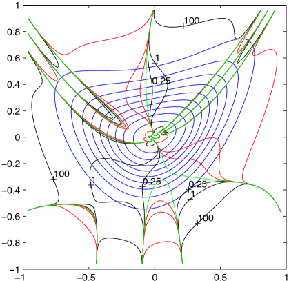
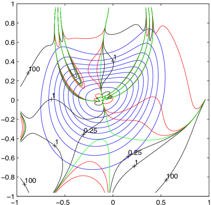
Figure 14: Contours 0.1,0.2,…,0.9 of a function are shown in blue, together with its invariant $\lambda_{n}$: contour 0 in green, contours $-0.25$, $-1$, and $-100$ in red, and contours 0.25, 1, and 100 in black. Top: function $f$ from (4.3). Bottom: Möbius related function $f\circ\varphi^{-1}$, parameters in (4.4). The invariance can be seen, along with the way that $\lambda_{n}$ typically blows up as $\nabla f\to 0$. A small discretization error is visible in the top figure: the saddle point near $(-0.5,-0.5)$ has $\lambda_{n}\approx 1.07$, whereas the exact value is 0.94. This results in the wrong topology of the $+1$ contour (cf. bottom figure near $(-0.8,-0.2)$).

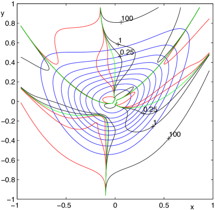
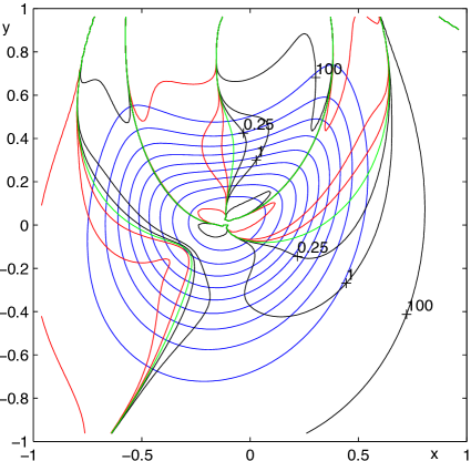
Figure 15: Contours 0.1,0.2,…,0.9 of a function are shown in blue, together with its invariant $\lambda_{t}$: contour 0 (which locates vertices (points of stationary curvature) of the level sets) in green, contours $-0.25$, $-1$, and $-100$ in red, and contours 0.25, 1, and 100 in black. Top: function $f$ from (4.3). Bottom: Möbius related function $f\circ\varphi^{-1}$, parameters in (4.4).

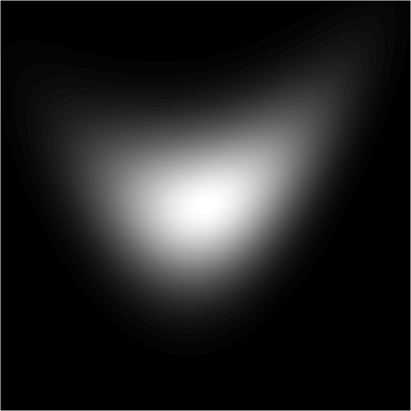
\begin{overpic}[width=411.93767pt]{blobhill} \put(75.0,-5.0){\small$-1$} \put(90.0,11.0){\small$x$} \put(102.0,25.0){\small$1$} \put(0.0,5.0){\small$1$} \put(30.0,0.0){\small$y$} \end{overpic}

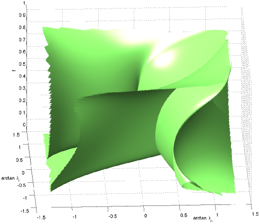
Figure 16: The sample image defined in equation (4.3) is shown in grayscale (top left) and as a graph $(x,y,f(x,y))$ (bottom left). Its Möbius signature surface (4.2) is shown at right.

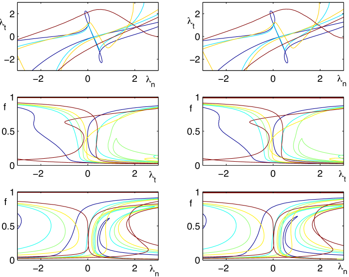
Figure 17: The invariant signature $(f,\lambda_{n},\lambda_{t})$ shown for $f$ in the left column and for $f\circ\varphi^{-1}$ in the right column. Top: contours 0.2, 0.4, 0.6, and 0.8 of $f$; middle and bottom: contours $-1$, $-0.25$, 0, 0.25, and 1 of $\lambda_{n}$ (resp. $\lambda_{t}$). The two invariants are almost identical in appearance (see, e.g., the $-1$ (dark blue) contour of $\lambda_{t}$ near $(\lambda_{n},f)=(1,0.6)$, which is slightly different in the left and right columns).

Example 4.3.

As a more numerical example, we take 9 similar blob-like functions, constructed as the sum of four random 2D Gaussian functions, and their Möbius images under a random Mobius transform, and compare their invariant signatures. The functions and their Mobius-transformed variants $f\circ\varphi^{-1}$ are shown in Fig. 18 as level set contours, while the invariant signatures are shown in Fig. 19. Because the whole invariant signature surfaces are very complicated, we show just the signature curve corresponding to the level set $f^{-1}(0.5)$. This depends only on the first 3 derivatives of $f$ on the level set. Because $\lambda_{n}$ and $\lambda_{t}$ take values in $[-\infty,\infty]$, we use coordinates $(\arctan(\lambda_{t}/4),\arctan(\lambda_{n}/4))$. Clearly, even this very limited portion of the signature serves to distinguish the Möbius-related pairs extremely sensitively. In some cases, the invariants change extremely rapidly along the level set, so that even though they are evaluated accurately, the resulting contours of the Möbius-related pairs do not overlap. This would need to be taken into account in the development of a distance measure on the invariant signatures.

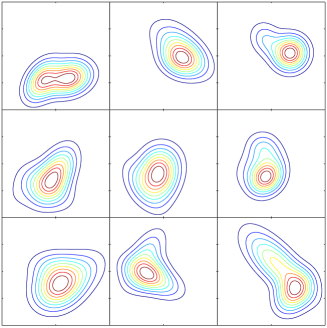
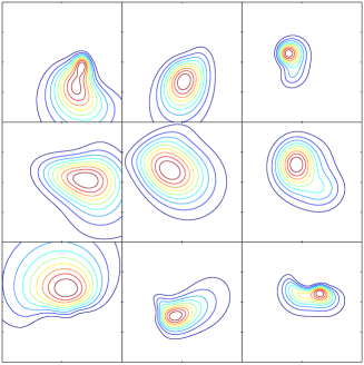
Figure 18: Nine random blob-like functions are shown on the left. Each is given by the sum of 4 random Gaussians, with the range of the resulting function scaled to $[0,1]$. The domain is $[-1,1]^{2}$ and the functions are discretized with $h=1/80$ giving $161\times 161$ grey-scale images. For each of the 9 functions $f$, a random Möbius transformation $\varphi$ is chosen and the composition $f\circ\varphi^{-1}$ shown on the right, evaluated on the domain $[-1,1]^{2}$. The transformations have parameters $b=0$, $a$ uniform in an annulus with inner radius 0.7 and outer radius 1.3, $d=1$, and $c$ with uniform argument and normal random modulus with standard deviation 0.6. The contours 0.1, 0.2,…,0.9 of the functions are shown.

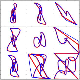
Figure 19: The invariant signature $(\arctan(\lambda_{t}/4),\arctan(\lambda_{n}/4))$ evaluated on the level set $f^{-1}(0.5)$ is calculated by central differences for each of the images in Fig. 18 left (shown in blue) and for the corresponding images in Fig. 18 right (shown in red). The domains are $[-\pi/2,\pi/2]^{2}$. The signature curves distinguish the Möbius-related pairs very sensitively; only tiny finite difference errors are visible. However, some errors related to insufficient resolution of the signature curves are clearly visible.

Example 4.4.

In this example we illustrate the extreme sensitivity of the invariant signature by evaluating it on 9 very similar images, together with their Möbius transformations. Each original image is a blob function generated as in Example 4.3, but with parameters varying only by $\pm 5\%$. The Möbius transformations have the form $1/(1+cz)$ where $c$ is normally distributed with standard deviation 0.1. The 0.5-level contours of the original and transformed images are shown in Fig. 20, and their signatures in Fig. 21. The signature is extremely sensitive to tiny changes in the image, but not to Möbius transformations.

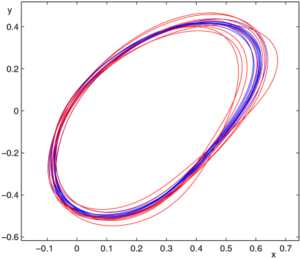
Figure 20: The 0.5-level contour of 9 very similar blob-like images are shown in blue, and of their Möbius transformations in red. Only the central $80\times 80$ portion of the $161\times 161$ images are shown.

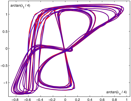
Figure 21: The invariant signature $(\arctan(\lambda_{t}/4),\arctan(\lambda_{n}/4))$ evaluated on the level set $f^{-1}(0.5)$ is shown for each of the images in Fig. 20 (blue) and for their Möbius transformations (red).

We do not have a full understanding of the properties of this invariant signature with respect to the criteria listed in Section 2. It is certainly fast, small, local, and lacks redundancy and suppression. It has a good numerical approximation on smooth (or smoothed) images. Is it complete? That is, given an image, does its signature surface determine the image up to a Möbius transformation? Suppose we are given a small piece of signature surface, parameterized by $(u,v)$, say. We are given three functions $\tilde{f}(u,v)$, $\tilde{\lambda}_{n}(u,v)$, and $\tilde{\lambda}_{t}(u,v)$, and need to determine (by solving three PDEs) three functions $f(x,y)$ (the image), $x(u,v)$, and $y(u,v)$ (the coordinates). Typically, the solution of these PDEs will be determined by some boundary data. This suggests that distinct images with the same signature are parameterized by functions of 1 variable; a kind of near completeness that may be good enough in practice.

Although very sensitive, the fact that it is not continuous at critical points means that it does not have good discrimination in the sense of Section 2. (It falls into the ‘more false negatives’ region of Fig. 1.) Near nondegenerate critical points, the signature blows up in a well-defined way, so it is possible that there exists a metric on signatures that leads to robustness and good discrimination.

5 Conclusion

In this paper we have developed Möbius invariants of both curves and images, and proposed computational methods to evaluate both, demonstrating them on a variety of examples. In Section 2 we identified a set of properties that are important for invariants, principally that there was a small set of invariants that were quick to compute, numerically stable, robust (so that noisy versions of the same curve have similar invariants) and yet sufficiently discriminatory (so that different objects have different invariants).

While differential invariants are not generally robust when dealing with noise, they offer good discrimination and are cheap to compute; this leads us to the Möbius arc-length. The cross-ratio is more robust, but requires a large set of points to be evaluated, and blows up as the pairs of points approach each other. In order to make this reparameterization-invariant, we used a Fourier transform. This lead to a method of computing Möbius invariants that satisfies the properties that we have outlined, as is demonstrated in the numerical experiments, see particularly Fig. 9.

For images, the extra information means that it is possible to compute a relatively simple three-dimensional signature based on the function value at each point together with two functions of the Möbius arclength, along and perpendicular to level sets of the image intensity. It is computationally cheap, extremely sensitive to non-Möbius changes in the image, but insensitive to Möbius transformations of the image.

Acknowledgements

This research was supported by the Marsden Fund, and RM by a James Cook Research Fellowship, both administered by the Royal Society of New Zealand. SM would like to thank the Erwin Schrödinger International Institute for Mathematical Physics, Vienna, where some of this research was performed.

References

- [1] Abu-Mostafa Y.S., Psaltis D., Recognitive aspects of moment invariants, IEEE Trans. Pattern Anal. Machine Intell. 6 (1984), 698–706.
- [2] Aghayan R., Ellis T., Dehmeshki J., Planar numerical signature theory applied to object recognition, J. Math. Imaging Vision 48 (2014), 583–605.
- [3] Ahlfors L.V., Cross-ratios and Schwarzian derivatives in , in Complex Analysis, Editors J. Hersch, A. Huber, Birkhäuser, Basel, 1988, 1–15.
- [4] Ames A.D., Jalkio J.A., Shakiban C., Three-dimensional object recognition using invariant Euclidean signature curves, in Analysis, Combinatorics and Computing, Nova Sci. Publ., Hauppauge, NY, 2002, 13–23.
- [5] Åström K., Fundamental difficulties with projective normalization of planar curves, in Applications of Invariance in Computer Vision, Lecture Notes in Computer Science, Vol. 825, Springer, Berlin – Heidelberg, 1994, 199–214.
- [6] Bandeira A.S., Cahill J., Mixon D.G., Nelson A.A., Saving phase: injectivity and stability for phase retrieval, Appl. Comput. Harmon. Anal. 37 (2014), 106–125, arXiv:1302.4618.
- [7] Barrett D.E., Bolt M., Cauchy integrals and Möbius geometry of curves, Asian J. Math. 11 (2007), 47–53.
- [8] Bauer M., Bruveris M., Michor P.W., Overview of the geometries of shape spaces and diffeomorphism groups, J. Math. Imaging Vision 50 (2014), 60–97, arXiv:1305.1150.
- [9] Calabi E., Olver P.J., Shakiban C., Tannenbaum A., Haker S., Differential and numerically invariant signature curves applied to object recognition, Int. J. Comput. Vis. 26 (1998), 107–135.
- [10] Edelsbrunner H., Harer J., Persistent homology – a survey, in Surveys on Discrete and Computational Geometry, Contemp. Math., Vol. 453, Amer. Math. Soc., Providence, RI, 2008, 257–282.
- [11] Feng S., Kogan I., Krim H., Classification of curves in 2D and 3D via affine integral signatures, Acta Appl. Math. 109 (2010), 903–937, arXiv:0806.1984.
- [12] Fridman B., Kuchment P., Lancaster K., Lissianoi S., Mogilevsky M., Ma D., Ponomarev I., Papanicolaou V., Numerical harmonic analysis on the hyperbolic plane, Appl. Anal. 76 (2000), 351–362.
- [13] Gauthier J.P., Smach F., Lemaître C., Miteran J., Finding invariants of group actions on function spaces, a general methodology from non-abelian harmonic analysis, in Mathematical Control Theory and Finance, Springer, Berlin, 2008, 161–186.
- [14] Ghorbel F., A complete invariant description for gray-level images by the harmonic analysis approach, Pattern Recognition Lett. 15 (1994), 1043–1051.
- [15] Glaunès J., Qiu A., Miller M.I., Younes L., Large deformation diffeomorphic metric curve mapping, Int. J. Comput. Vis. 80 (2008), 317–336.
- [16] Hann C.E., Hickman M.S., Projective curvature and integral invariants, Acta Appl. Math. 74 (2002), 177–193.
- [17] Hickman M.S., Euclidean signature curves, J. Math. Imaging Vision 43 (2012), 206–213.
- [18] Hoff D.J., Olver P.J., Extensions of invariant signatures for object recognition, J. Math. Imaging Vision 45 (2013), 176–185.
- [19] Kakarala R., The bispectrum as a source of phase-sensitive invariants for Fourier descriptors: a group-theoretic approach, J. Math. Imaging Vision 44 (2012), 341–353, arXiv:0902.0196.
- [20] Lenz R., Group theoretical methods in image processing, Lecture Notes in Computer Science, Vol. 413, Springer-Verlag, Berlin, 1990.
- [21] Manay S., Cremers D., Hong B., Yezzi A.J., Soatto S., Integral invariants for shape matching, IEEE Trans. Pattern Anal. Machine Intell. 28 (2006), 1602–1618.
- [22] Marsland S., McLachlan R.I., Modin K., Perlmutter M., Geodesic warps by conformal mappings, Int. J. Comput. Vis. 105 (2013), 144–154, arXiv:1203.3982.
- [23] Michor P.W., Manifolds of differentiable mappings, Shiva Mathematics Series, Vol. 3, Shiva Publishing Ltd., Nantwich, 1980.
- [24] Michor P.W., Mumford D., An overview of the Riemannian metrics on spaces of curves using the Hamiltonian approach, Appl. Comput. Harmon. Anal. 23 (2007), 74–113, math.DG/0605009.
- [25] Milnor J.W., The geometry of growth and form, Talk given at the IAS, Princeton, 2010, available at http://www.math.sunysb.edu/~jack/gfp-print.pdf.
- [26] Mumford D., Pattern theory and vision, in Questions Mathématiques En Traitement Du Signal et de L’Image, Chapter 3, Institute Henri Poincaré, Paris, 1998, 7–13.
- [27] O’Hara J., Solanes G., Möbius invariant energies and average linking with circles, Tohoku Math. J. 67 (2015), 51–82, arXiv:1010.3764.
- [28] Olver P.J., Moving frames and singularities of prolonged group actions, Selecta Math. (N.S.) 6 (2000), 41–77.
- [29] Olver P.J., Joint invariant signatures, Found. Comput. Math. 1 (2001), 3–67.
- [30] Olver P.J., Moving frames – in geometry, algebra, computer vision, and numerical analysis, in Foundations of Computational Mathematics (Oxford, 1999), London Math. Soc. Lecture Note Ser., Vol. 284, Cambridge University Press, Cambridge, 2001, 267–297.
- [31] Olver P.J., A survey of moving frames, in Computer Algebra and Geometric Algebra with Applications, Lecture Notes in Computer Science, Vol. 3519, Springer, Berlin – Heidelberg, 2005, 105–138.
- [32] Olver P.J., The symmetry groupoid and weighted signature of a geometric object, J. Lie Theory 26 (2016), 235–267.
- [33] Patterson B.C., The differential invariants of inversive geometry, Amer. J. Math. 50 (1928), 553–568.
- [34] Petukhov S.V., Non-Euclidean geometries and algorithms of living bodies, Comput. Math. Appl. 17 (1989), 505–534.
- [35] Shakiban C., Lloyd P., Signature curves statistics of DNA supercoils, in Geometry, Integrability and Quantization, Softex, Sofia, 2004, 203–210.
- [36] Shakiban C., Lloyd P., Classification of signature curves using latent semantic analysis, in Computer Algebra and Geometric Algebra with Applications, Lecture Notes in Computer Science, Vol. 3519, Springer, Berlin – Heidelberg, 2005, 152–162.
- [37] Taylor M.E., Noncommutative harmonic analysis, Mathematical Surveys and Monographs, Vol. 22, Amer. Math. Soc., Providence, RI, 1986.
- [38] Thompson D.W., On growth and form, Cambridge University Press, Cambridge, England, 1942.
- [39] Turski J., Geometric Fourier analysis of the conformal camera for active vision, SIAM Rev. 46 (2004), 230–255.
- [40] Turski J., Geometric Fourier analysis for computational vision, J. Fourier Anal. Appl. 11 (2005), 1–23.
- [41] Turski J., Computational harmonic analysis for human and robotic vision systems, Neurocomputing 69 (2006), 1277–1280.
- [42] Van Gool L., Moons T., Pauwels E., Oosterlinck A., Vision and Lie’s approach to invariance, Image Vision Comput. 13 (1995), 259–277.
- [43] Wallace A., D’Arcy Thompson and the theory of transformations, Nature Rev. Genet. 7 (2006), 401–406.