Noisy Branes

Abstract

We study the effects of disorder on strongly coupled compressible matter in 2+1 dimensions. Our system consists of a D3/D5 intersection at finite temperature and in the presence of a disordered chemical potential. We first study the impact of disorder on the charge density and the quark condensate. Next, we focus on the DC conductivity and derive analytic expressions for the corrections induced by weak disorder. It is found that disorder enhances the DC conductivity at low charge density, while for large charge density the conductivity is reduced. We present numerical simulations both for weak and strong disorder. Finally, we show how disorder gives rise to a sublinear behavior for the conductivity as a function of the charge density, a behavior qualitatively similar to predictions and observations for electric transport in graphene.

1 Introduction

The interplay of disorder and strong interactions is a challenging problem in Condensed Matter, with a wide range of potential applications from High-Tc superconductors Pan_Nature ; Renner_Nature to graphene PhysRevLett.99.246803 ; PhysRevLett.98.186806 . At the theoretical level it poses important questions as the existence and nature of disordered quantum critical points PhysRevB.27.413 ; 0305-4470-39-22-R01 , and the possibility of disorder-induced metal to insulator phase transitions for strongly interacting systems.

Gauge/Gravity duality is a promising venue to address strongly coupled problems in Condensed Matter, and the last years have seen interesting progress towards a description of disordered strongly coupled systems. These advances include holographic models of disordered fixed points Hartnoll:2014cua ; Garcia-Garcia:2015crx , disordered superconductors Arean:2014oaa ; Arean:2013mta , and hyperscaling violating geometries, which are promising candidates to duals of strange metals, deformed by disordered sources Lucas:2014zea .

A natural procedure to characterize the effects of disorder is to study the transport properties of the system, and in particular the electrical conductivity. Compelling results for the transport properties of solutions dual to theories with disorder have been obtained, mainly through numerical solutions of Einstein plus matter theories Donos:2014yya ; Hartnoll:2015rza , but also via analytic computations at weak disorder O'Keeffe:2015awa ; Garcia-Garcia:2015crx . Finally, hydrodynamic models of strongly coupled disordered systems have led to promising results like the fitting of experimental data for graphene Lucas:2015sya , or the description of phase disordered superconducting phase transitions Davison:2016hno .

All the holographic models dual to disordered theories we have described above, and the majority of those constructed thus far, are of the so-called bottom-up type. They are effective models whose Lagrangian is not derived from a solution of String Theory, or Supergravity, and thus lack a microscopic description. In this note we will instead implement disorder in a top-down model that has been one of the workhorses of Gauge/Gravity duality applications to QCD-like theories; that of probe branes Karch:2002sh . We will consider a D5-brane probe embedded in the geometry generated by $N_{c}$ D3-branes: the D5 shares two spatial directions with the D3s, and introduces fundamental degrees of freedom, quarks, along a (2+1)-dimensional defect in the theory dual to $N_{c}$ D3-branes. More precisely, for $N_{f}$ D5-brane probes, the system is dual to ${\cal N}=4$ $SU(N_{c})$ SYM with $N_{f}$ ${\cal N}=2$ matter hypermultiplets living on a (2+1)-dimensional defect Karch:2000gx ; DeWolfe:2001pq . Since we are interested in systems at finite temperature and charge density, we will work with the black hole background generated by black D3-branes, and add charge density by switching on the temporal component of the gauge field living on the worldvolume of the D5-brane Kobayashi:2006sb ; Evans:2008nf .

The implementation of disorder via a probe brane model was considered for the first time in Ryu:2011vq , and subsequently in Ikeda:2016rqh , where it was shown that the DC conductivity is bounded, and, as a consequence, an insulating phase is excluded from this scenario. However, it is in this work that for the first time disorder is implemented explicitly in a top-down holographic model of probe branes. We construct disordered embeddings of a probe D5-brane in a black D3-background by switching on a disordered chemical potential on the worldvolume of the probe. The analysis of those embeddings, and the study of their fluctuations has produced the following results

• We construct both massive and massless inhomogeneous embeddings characterized by a disordered chemical potential, and compute their charge density and, for the massive case, also the value of the quark condensate.

• We study the effects of disorder on the charge density and the quark condensate using analytic and numerical methods. Two regimes are found: at small charge density the quark condensate scales quadratically with the strength of disorder, while the charge density is almost independent of that disorder strength. For large charge density the converse happens: the quark condensate is largely unaffected by disorder while the charge density scales quadratically with the disorder strength.

• We express the DC conductivity, $\sigma_{\rm DC}$, in terms of horizon data and obtain analytic expressions for $\sigma_{\rm DC}$ in a small disorder regime. For small charge density $\sigma_{\rm DC}$ is enhanced by disorder. For large charge density, $\sigma_{\rm DC}$ decreases with the disorder strength. Numerical simulations, which agree with the analytic predictions, confirm this scenario.

• We compute the dependence of $\sigma_{\rm DC}$ on the charge density via numerical simulations, and analytic approximations. At weak disorder $\sigma_{\rm DC}$ scales linearly with the charge density (except at very low charge density), with a slope that is reduced as the noise strength is increased. At strong disorder the dependence of $\sigma_{\rm DC}$ on the charge density becomes sublinear. This last behavior shows similarities to that observed in graphene near the charge neutrality point. Finally, we observe that the analytic, or semi-analytical, approximations agree very well with the numerical simulations.

• We study the spectral properties of the system by considering a noise characterized by a Fourier power spectrum of the form $1/k^{2\alpha}$. The resulting power spectra for the charge density and the quark condensate are found to be of the form $1/k^{2\alpha-2}$ and $1/k^{2\alpha+6}$ respectively. With respect to the input power spectrum, our holographic model smooths out the quark condensate, while it makes the charge density more irregular.

The rest of this paper is organized as follows. Section 2 is devoted to the construction of disordered embeddings of a probe D5-brane: in Sec. 2.1 we introduce the background geometry, and in Sec. 2.2 we write down the action and asymptotics for the embedding of the probe D5-brane. The disordered chemical potential is described in Sec. 2.3, and the numerical methods used to construct the embeddings are discussed in Sec. 2.4. In Section 2.5 we present the numerical results for the embeddings and discuss the effects of disorder on the charge density and the quark condensate. Sec. 3 is dedicated to the study of the electrical conductivity. In Sec. 3.1 we compute the DC conductivity in terms of horizon data, and in Sec. 3.2 we derive analytic expressions for $\sigma_{\rm DC}$ in a small noise expansion. In Sec. 3.3 we introduce a semi-analytical approach to $\sigma_{\rm DC}$ valid at all orders in the strength of noise, and obtain predictions for the behavior of $\sigma_{\rm DC}$ at strong noise. In Sec. 3.4 we present our numerical results for $\sigma_{\rm DC}$ and compare them with the analytic predictions, paying special attention in Sec. 3.4.1 to the behavior of $\sigma_{\rm DC}$ as a function of $\langle\rho\rangle$. Finally, in Section 4 we analyze the spectral properties of the system. We conclude in Sec. 5 with a summary of our results and a review of the ways forward this work opens. We have included three appendices in this manuscript: App. A is dedicated to the homogeneous version of our model (i.e. without disorder). In App. B we discuss the reliability of our numerics against the lattice size, and present supplementary results for strong disorder. In App. C we show numerical embeddings for the case of a disorder characterized by a Fourier power spectrum $\sim 1/k^{2\alpha}$.

2 Disordered D3/D5 intersection

Our setup is built upon the supersymmetric intersection of $N_{c}$ D3- and $N_{f}$ D5-branes along 2+1 spacetime dimensions, which is dual to (3+1)-dimensional ${\cal N}=4$ SYM with $N_{f}$ fundamental hypermultiplets living on a (2+1)-dimensional defect Karch:2000gx ; DeWolfe:2001pq . We work in the probe limit $N_{f}\ll N_{c}$, and hence consider a probe D5-brane in the background generated by $N_{c}$ D3-branes. Moreover, we are interested in systems at finite temperature and with a nonzero density of the fundamental degrees of freedom realized by the strings stretched between the D3- and D5-branes.

2.1 Background

The metric of the geometry generated by $N_{c}$ black D3-branes can be written as

$$ds^{2}=\frac{L^{2}}{z^{2}}\left(-\frac{f(z)^{2}}{h(z)}\,dt^{2}+h(z)\,d\vec{x}^{2}+dz^{2}\right)+L^{2}\,d\Omega_{5}^{2}\,,$$ (2.1)

$${\rm with}\quad f(z)=1-z^{4}\,,\qquad h(z)=1+z^{4}\,,$$ (2.2)

where we are following the conventions of Araujo:2015hna , and we have performed a rescaling that sends the horizon radius $z_{0}$ to the unity. Remember that the temperature of the black hole is determined in terms of $z_{0}$ as $T=\sqrt{2}/(\pi\,z_{0})$. It is straightforward to check that this metric is asymptotic, as $z\to 0$, to $AdS_{5}\times S^{5}$, and one should recall that the AdS radius $L$, the number of D3-branes, $N_{c}$, the string tension $(2\pi\alpha^{\prime})^{-1}$, and the coupling constant of the dual theory, $g_{\rm YM}$, are related via $L^{4}/\alpha^{\prime 2}=2g_{\rm YM}^{2}\,N_{c}\equiv 2\lambda$, where $\lambda$ is the ’t Hooft coupling. This background possesses a nonzero RR five form given by $d{\rm Vol}(S^{5})+{\rm h.d.}$, which will not play any role in this setup.

2.2 Embedding

The probe D5-brane is extended along two Minkowski directions, say $(x,y)$, the radial coordinate $z$, and wraps an $S^{2}$ inside the internal $S^{5}$ whose metric can be written as

$$d\Omega_{5}^{2}=d\theta^{2}+\sin^{2}\theta\,d\Omega_{2}^{2}+\cos^{2}\theta\,d\tilde{\Omega}_{2}^{2}\,,$$ (2.3)

where $\Omega_{2}$ is the volume element of the $S^{2}$ wrapped by the probe brane, and the D5 sits at a fixed point of the remaining $S^{2}$. The embedding can then be described in terms of the coordinate $\theta$ determining the radius of the $S^{2}$ wrapped by the probe. For simplicity we will work in terms of $\chi=\cos\theta$.

We will study configurations with finite charge density of the fundamental fields introduced by the D5-brane, and hence we must turn on the temporal component of the $U(1)$ worldvolume gauge field. Moreover, we want to describe a system where the charge density depends on one of the spatial directions, which we choose to be $x$. Therefore, the embedding is described in terms of the fields

$$\chi(z,x)\,,\quad A_{t}={L^{2}\over 2\pi\,\alpha^{\prime}\,z_{0}}\,\phi(z,x)\,,$$ (2.4)

where as in Araujo:2015hna we have written $A_{t}$ in terms of a conveniently dimensionless field $\phi$. The action is given by the DBI for the probe D5-brane, and takes the form

$${{\cal S}\over N_{f}\,T_{D5}\,L^{6}}=-\int dt\,d^{2}x\,dz\,d\Omega_{2}\,f\,z^{-4}\,\sqrt{h\,(1-\chi^{2})\,(S_{\chi}+S_{\phi}+S_{\text{int}})}\,,$$ (2.5)

with

$$S_{\chi}=1-\chi^{2}+z^{2}\chi^{\prime 2}+\frac{z^{2}\,\dot{\chi}^{2}}{h}\,,$$

$$S_{\phi}=-\frac{z^{4}(1-\chi^{2})}{f^{2}}\left(h\,\phi^{\prime 2}+\dot{\phi}^{2}\right)\,,$$

$$S_{\text{int}}=-\frac{z^{6}(\dot{\chi}\phi^{\prime}-\chi^{\prime}\dot{\phi})^{2}}{f^{2}}\,,$$ (2.6)

where the tilde and the dot denote a partial derivative with respect to $z$ and $x$ respectively. The equations of motion for $\chi(z,x)$ and $\phi(z,x)$ follow readily from this action, and they have been written explicitly in the appendix of Araujo:2015hna . In the last part of this work we will consider massless embeddings corresponding to $\chi(z,x)=0$. In that case the equation of motion for $\chi(z,x)$ is trivially satisfied, while that for $\phi(z,x)$ takes the form

$$z^{3}\left[\dot{\phi}^{2}\left(\phi^{\prime}\left(3z\,h^{\prime}-4h\right)+2h\,z\,\phi^{\prime\prime}\right)-4h\,z\,\dot{\phi}\,\phi^{\prime}\,\overset{.}{\phi^{\prime}}+2h\left(\phi^{\prime}\right)^{2}\left(z\,\ddot{\phi}+\phi^{\prime}\left(z\,h^{\prime}-2h\right)\right)\right]$$

$$\quad-f^{2}\left(2\ddot{\phi}+3h^{\prime}\,\phi^{\prime}+2h\,\phi^{\prime\prime}\right)+2f\,h\,f^{\prime}\,\phi^{\prime}=0\,.$$ (2.7)

One can read the observables of the dual theory from the UV asymptotics of the embedding fields. These result from solving the equations of motion in the $z\to 0$ limit, and read

$$\phi(z,x)=\mu(x)-\rho(x)z+{\cal O}(z^{2})\,,$$ (2.8a)

$$\chi(z,x)=m(x)\,z+c(x)z^{2}+{\cal O}(z^{3})\,,$$ (2.8b)

where $\mu$, $\rho$, $m$, and $c$ determine the chemical potential, charge density, quark mass, and quark condensate respectively. Proceeding as in Araujo:2015hna we plug in the dimensionful constants, and define the quark mass $M_{q}=\sqrt{\lambda}\,\bar{M}$, where $\bar{M}=m/z_{0}$. We then arrive to

$$m={2\sqrt{2}\over\pi\sqrt{\lambda}}\,{M_{q}\over T}\,,\qquad\mu={2\over\sqrt{\lambda}}\,{\bar{\mu}\over T}\,,\qquad\rho={2\sqrt{2}\over\pi\sqrt{\lambda}}\,{\bar{\rho}\over T^{2}}\,,$$ (2.9)

where $\bar{\mu}$ and $\bar{\rho}$ are the dimensionful chemical potential and charge density respectively. Moreover, as discussed with detail in Mateos:2007vn , $c$ is proportional to the condensate of the supersymmetric version of the quark bilinear ${\cal O}_{m}=\bar{\psi}\,\psi+\dots$, (the dots stand for terms including the superpartners of $\psi$)

$$c=-{1\over N_{f}\,N_{c}}{\langle{\cal O}_{m}\rangle\over T^{2}}\,.$$ (2.10)

We will work at fixed $\mu$ and $m$. The phase diagram of the homogeneous D3/D5 setup was studied in Evans:2008nf , and reviewed in Araujo:2015hna in terms of $\mu$ and $m$. As first explained in Kobayashi:2006sb , at finite charge density only black hole embeddings exist. These are embeddings for which the probe brane intersects the horizon.

Finally, we shall study the IR asymptotics of our system. Imposing regularity at the black hole horizon, it is straightforward to check that in its vicinity the solutions for the embedding fields take the form

$$\phi(z,x)=a^{(2)}(x)\,(1-z)^{2}+{\cal O}((1-z)^{3})\,,$$ (2.11a)

$$\chi(z,x)=C^{(0)}(x)+C^{(2)}(x)\,(1-z)^{2}+{\cal O}((1-z)^{3})\,,$$ (2.11b)

where $C^{(2)}(x)$ is a function of $C^{(0)}(x)$ and $a^{(2)}(x)$ as shown in Araujo:2015hna .

2.3 Disordered $\mu$

To mimic a random on-site potential as that used originally by Anderson Anderson:1958vr , we introduce a noisy chemical potential of the form

$$\mu(x)=\mu_{0}+{\mu_{0}\over 25}\,w\,\sum_{k=k_{0}}^{k_{*}}\,\cos(k\,x+\delta_{k})\,,$$ (2.12)

with $\delta_{k}$ being a random phase for each wave number $k$, and $w$ a parameter that determines the strength of the noise. This chemical potential does not depend on $y$, hence our setup is homogeneous along this remaining spatial direction. We discretize the space along $x$ and impose periodic boundary conditions in that direction, which results in $k$ taking the values

$$k_{n}={2\pi\over L_{x}}\,(n+1)\quad{\rm with}\quad 0\leq n<N=\frac{k_{*}}{k_{0}}\,,$$ (2.13)

where $L_{x}$ is the length of the (cylindrical) system along $x$. Notice that this noise is a truncated version of Gaussian white noise. The highest wave number, $k_{*}$, plays the role of the inverse of the correlation length for the chemical potential, while the lower wave number, $k_{0}$, is proportional to the inverse of the system size. Moreover, for a lattice with $N_{x}$ sites along the $x$ direction,

$$k_{*}\leq k_{\rm ns}\equiv\frac{\pi}{L_{x}}\,(N_{x}-1),$$ (2.14)

where $k_{\rm ns}$ is the Nyquist frequency for that lattice. The properties of this choice of disorder have been discussed in more detail in Arean:2014oaa . We will specify our choice of parameters when discussing the numerical integration.

2.4 Numerics

To construct the embeddings we will solve numerically the equations of motion resulting from (2.5). These are two coupled PDEs depending on $z$ and $x$. To solve them numerically we discretize the space along both directions, and impose periodic boundary conditions along $x$. As for the radial direction, in the UV we have the asymptotic solution (2.8), while in the IR ($z\to 1$) the requirement of regularity at the black hole horizon imposes that $\phi$ and $\chi^{\prime}$ vanish there (see Eq. (2.11)). Therefore, we impose the following boundary conditions

$$\phi(0,x)=\mu(x)\,,\qquad\chi^{\prime}(0,x)=m\,,$$ (2.15a)

$$\phi(1,x)=0\,,\qquad\quad\;\;\chi^{\prime}(1,0)=0\,.$$ (2.15b)

We use pseudospectral methods implemented in Mathematica, discretizing the plane $(z,x)$ on a rectangular lattice of size $N_{z}\times N_{x}$, with $N_{z}$ and $N_{x}$ being, respectively, the number of points in the $z$ and $x$ directions. We use a Chebyshev grid along $z$, and a planar one in the $x$ direction; and employ a Newton-Raphson iterative algorithm to solve the resulting nonlinear algebraic equations. For all the numerical simulations apart from those in Sec. 4 we set $L_{x}=20\pi$, so that $k_{0}/T\ll 1$, and take $k_{*}=1$ which corresponds to truncating the sum in (2.12) at 10 modes. Finally, we average over different realizations of the noisy chemical potential. When it is visible we show the error of the average $\sigma_{N}/\sqrt{N}$, where $\sigma_{N}$ is the standard deviation, and $N$ the number of realizations. Only in Fig. 8 we plot the standard deviation instead of the error of the average.

2.5 Results

Let us first consider massless embeddings; for these the embedding field $\chi$ vanishes, and we need only solve the equation of motion for $\phi$.

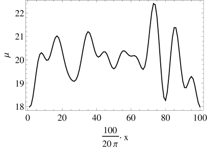
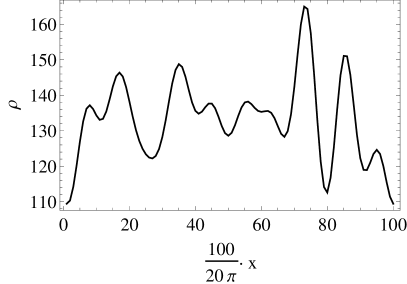
Figure 1: Massless embedding. On the left panel we plot an example of one realization of $\mu(x)$ with $\mu_{0}=20$ and $w=0.5$. On the right we present the corresponding charge density for a massless embedding with that chemical potential. We have employed a lattice of size $100\times 100$ and set $L_{x}=20\pi$, $k_{*}=1$.

In Fig. 1 we plot the result of a single simulation of our noisy system. We present the random chemical potential we plug in as our boundary condition together with the resulting charge density which we read from the asymptotic behavior of the worldvolume field $\phi$.

Charge Density

It is interesting to study how the charge density depends on the strength of disorder. An important observable of our setup is given by the spatial average of the charge density, $\langle\rho\rangle$ (we will denote by $\langle\cdot\rangle$ the average over the spatial direction $x$). Therefore, for a noisy chemical potential as (2.12), we will analyze how $\langle\rho\rangle$ depends on the strength of the noise, parametrized by $w$. The expected behavior can be anticipated by considering how the charge density depends on the chemical potential in the homogeneous case. In App. A we have reviewed the homogeneous D3/D5 intersection, and in particular we have shown that the function $\mu(\rho)$ can be computed analytically, and is given by Eq. (A.32). That function interpolates between two distinct behaviors as shown in (A.34); while $\rho\sim\mu^{2}$ for large $\rho$, $\rho\sim\mu$ in the small $\rho$ limit. Assuming this behavior holds for an $x$ dependent noisy $\mu$ as (2.12), it is easy to predict how $\langle\rho\rangle$ should behave as a function of $w$. First, in the low $\rho$ regime, where $\rho\sim\mu$, taking into account that the noisy $x$ dependent part of (2.12) averages to zero, one concludes that $\langle\rho\rangle$ must be independent of $w$. Instead, at large $\rho$, where we assume $\rho\sim\mu^{2}$, one expects $\langle\rho\rangle\sim w^{2}$ (we will show this explicitly in Eq. (3.26) below).

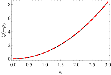
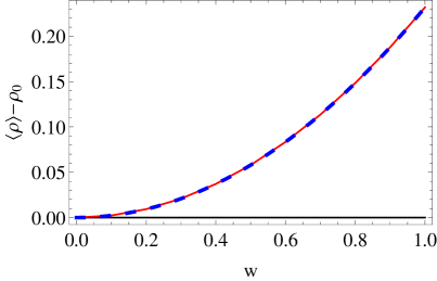
Figure 2: $\langle\rho\rangle$ versus $w$. On the left we plot $\langle\rho\rangle-\rho_{0}$ for a system with $\mu_{0}=20$, $\rho_{0}=133.398$ is the value of $\rho$ for the clean case. The black line shows the result of the numerical integration, and the red dashed line the fit $\log(\langle\rho\rangle-\rho_{0})=-0.0726+2.000\log(w)$. On the right panel we plot the subtracted charge density for $\mu_{0}=10$ (red line, $\rho_{0}=38.897$), and $\mu_{0}=0.1$ (black line, $\rho_{0}=0.141$). The blue dashed line results from the fit $\log(\langle\rho\rangle-\rho_{0})=-1.462+2.000\log(w)$ to the $\mu_{0}=10$ data. For both graphs we have averaged over 10 realizations on a lattice of size $100\times 100$ and set $L_{x}=20\pi$, $k_{*}=1$.

In Fig. 2 we present the results of our numerical simulations for the evolution of the averaged charge density as a function of the disorder strength. First, on the left panel we plot $\langle\rho\rangle$ versus $w$ for a system with $\mu_{0}=20$, which corresponds to $\rho_{0}\approx 133.398$, and places the setup in the large charge density regime. As expected $\langle\rho\rangle$ scales quadratically with $w$ as the fit in the graph demonstrates. Next, on the right plot we show two cases corresponding to lower charge density, namely $\mu_{0}=10$ (red line), and $\mu_{0}=0.1$ (black line), for which $\rho_{0}$ takes the values 38.897, and 0.141 respectively. While for $\mu_{0}=10$, the quadratic scaling of $\langle\rho\rangle$ is still observed, for $\mu_{0}=0.1$ we see that the averaged charge density is independent of the noise strength.

In the remaining of this section we consider the case of nonzero mass. We then have to solve the two coupled PDEs for $\phi$ and $\chi$. When choosing the value of the mass $m$ one has to take into account the phase diagram for black hole embeddings at finite charge density and nonzero mass, which was reviewed in Araujo:2015hna . In particular, notice that for $m\gtrsim 1.5$, black hole embeddings exist only for $\mu\gtrsim m-1.41$. We will restrict our analysis to cases where the space dependent chemical potential never reaches that forbidden region. In Fig. 3 we plot the result of a simulation for a massive embedding, showing the noisy chemical potential that we impose as boundary condition, and the resulting charge density and quark condensate we read from the solution of the PDEs.

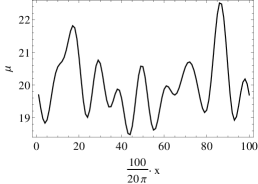
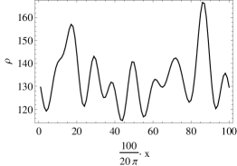
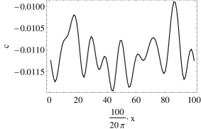
Figure 3: Massive embedding. The three panels display, from left to right, the chemical potential $\mu(x)$, the charge density $\rho(x)$, and the quark condensate $c(x)$ for a simulation with $\mu_{0}=20$, $m=0.5$, $w=0.5$, $L_{x}=20\pi$, and $k_{*}=1$ (corresponding to 10 modes) on a lattice of size $100\times 100$.

Quark Condensate

The construction of disordered massive embeddings offers us the possibility of looking into the behavior of the quark condensate $c$ in presence of disorder. As above, much can be inferred from the behavior of the homogeneous brane intersection. For massive embeddings there is no analytical solution that allows us to express $c$ in terms of $\mu$, and instead, as we show in App. A, one needs to solve numerically a single ordinary differential equation for $\chi(z)$. However, one can obtain analytic (or semi-analytical) expressions for the dependence of $c$ on $\mu$ in the limits of large and small chemical potential. These are Eqs. (A.16) for $\mu\ll 1$, and (A.27) for $\mu\to\infty$. Those equations reflect two different scaling regimes: $c$ scales as $\mu^{2}$ for small $\mu$, while it becomes linear in $\mu$ as $\mu\to\infty$. The numerical integration confirms these two regimes as is illustrated on the left panel of Fig. 4. Notice that for an homogeneous embedding with mass $m=0.5$, Eqs. (A.16) and (A.27) result in the following behavior of the quark condensate as a function of $\mu$

$$\log_{10}(c(0)-c(\mu))=2\,\log_{10}\mu-1.170\,;\qquad(\mu\to 0)\,,$$ (2.16a)

$$\log_{10}(c(0)-c(\mu))=\log_{10}\mu-0.837\,;\qquad(\mu\to\infty)\,,$$ (2.16b)

which agrees with the fit to the numerical data in Fig. 4 (see caption). Therefore, an opposite scenario to that of the charge density above is anticipated for the dependence of $\langle c\rangle$ on the noise strength $w$. While for low $\mu_{0}$ we expect $\langle c\rangle$ to scale quadratically with $w$, for large $\mu_{0}$, the averaged quark condensate should become largely independent of the noise strength. These expectations are confirmed by our numerical simulations presented on the right hand side of Fig. 4. There we plot the subtracted quark condensate (denoting $c_{0}$ the value of $c$ at zero disorder) for systems with $\mu_{0}=1.5$ (black line) and $\mu_{0}=20$ (red line).

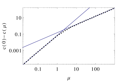
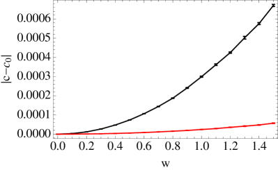
Figure 4: Massive embedding. On the left we plot the behavior of the homogeneous condensate $c$ as a function of the chemical potential $\mu$ for a fixed mass $m=0.5$. The fits are $\log_{10}(c(0)-c(\mu))=2.004\log_{10}\mu-1.170$, and $\log_{10}(c(0)-c(\mu))=1.003\log_{10}\mu-0.847$. The right panel shows the subtracted condensate $c-c_{0}$ versus the noise strength $w$ for $\mu_{0}=1.5$ (black) and $\mu_{0}=20$ (red), with $m=0.5$ in both cases. For the clean system ($w=0$) the condensate takes the value $c_{0}=-0.431$ ($c_{0}=-3.114$) for the case $\mu_{0}=1.5$ ($\mu_{0}=20$). We have averaged over 10 realizations on a grid of size $100\times 100$, and set $L_{x}=20\pi$, $k_{*}=1$.

One could repeat the analysis for the dependence of the charge density on the strength of disorder for the case of massive embeddings. However, Eqs. (A.15) and (A.26) show that the scaling of $\rho$ with $\mu$ in the homogeneous case is the same as for massless embeddings. Therefore, the behavior of $\rho$ as a function of $w$ is qualitatively the same as for the massless case examined above.

3 Noisy Conductivity

In this section we will study the electrical transport properties of our setup. We will focus on the study of the electrical conductivity in the direction parallel to the noise, namely $\sigma_{xx}\equiv\sigma$, and in particular its DC (zero frequency) value. To compute that conductivity we need to consider fluctuations of the worldvolume gauge field $A_{x}$ realizing an electric current along $x$. In general those fluctuations will source other fields in the model, and one has to solve a system of coupled linear PDEs.

The ansatz for the fluctuating field is

$$A_{\mu}=a_{\mu}(z,x)\,e^{i\omega\,t}\,,$$ (3.1)

and we will require that $f_{tx}(0,x)=i\omega\,e^{i\omega\,t}$, so that on the boundary the fluctuation is sourcing an oscillating electric field with constant modulus. The AdS/CFT dictionary tells us to compute the conductivity as

$$\sigma=\frac{J_{x}}{E_{x}}=\lim_{z\to 0}\frac{f_{xz}}{f_{tx}}\,.$$ (3.2)

Hence, we need to solve the equations of motion resulting from the expansion of the DBI action up to quadratic order in the fluctuations. These equations couple $a_{x}(z,x)$ to the fluctuation of the temporal component of the gauge field, $a_{t}(z,x)$, and in the massive case also to the fluctuation of the embedding field $\chi$, which we will denote $c(z,x)$. Moreover, we choose to work in the gauge $a_{z}(z,x)=0$. The quadratic action for these fluctuating fields has been written in the appendix of Araujo:2015hna . To compute the AC conductivity one then needs to solve the resulting system of linear PDEs. Since the background is periodic along $x$, one has to impose periodic boundary conditions in that direction. As for the radial direction, in the UV one requires

$$f_{tx}(0,x)=i\omega\,e^{i\omega\,t}\,,\qquad c^{\prime}(0,x)=0\,,$$

$$i\omega\,\partial_{z}a_{t}(0,x)-\partial_{x}\partial_{z}a_{x}(0,x)=0\,.$$ (3.3)

The first condition corresponds to switching on a constant electric on the boundary, while the second ensures that no fluctuation of the mass of the quarks is sourced. The third equation is a constraint resulting from the equation of motion for $a_{z}$, and upon substituting the form of the UV asymptotics amounts to the equation for charge conservation on the boundary Araujo:2015hna . In particular, that equation implies that at zero frequency the electric current in the $x$ direction, $J_{x}=-\partial_{z}a_{x}(0,x)$, is independent of $x$. Consequently, the DC conductivity in that direction is a constant.

In the IR one must impose infalling boundary conditions at the horizon. The IR behavior of the fluctuations was also studied in Araujo:2015hna , and it is straightforward to check that the resulting conditions to impose read

$$\tilde{a}_{t}(1,x)=0\,,\quad\tilde{a}_{x}^{\prime}(1,x)=-\frac{i\omega}{4\sqrt{2}}\,\tilde{a}_{x}(1,x)\,,$$

$$\tilde{c}^{\prime}(1,x)=-\frac{i\omega}{4\sqrt{2}}\,\tilde{c}(1,x)\,,$$ (3.4)

where we have redefined the fields as $\tilde{\Phi}=(1-z)^{-i\omega\over 2\sqrt{2}}\,\Phi$.

In this work we will not present results for the AC conductivity, and will instead focus our attention on the $\omega=0$ DC conductivity. Crucially, as was shown in Araujo:2015hna , the DC conductivity for this system can be computed without having to solve for the fluctuations we have just described.

3.1 DC Conductivity

The DBI action governing the fluctuations allows us to follow the procedure of Iqbal:2008by ; Ryu:2011vq , and express the DC conductivity, $\sigma_{\rm DC}$, in terms of the background functions, $\phi$ and $\chi$, evaluated at the horizon. In Araujo:2015hna that computation was particularized to a D3/D5 intersection like the one in our setup, obtaining for $\sigma_{\rm DC}$

$$\sigma_{\rm DC}={L_{x}\over\int_{0}^{L_{x}}\frac{dx}{{\cal F}(1,x)}}\,,$$ (3.5)

where ${\cal F}$ is the following function of the embedding fields $\phi$ and $\chi$, and the metric functions $f$ and $h$

$${\cal F}(z,x)=f\left(1-\chi^{2}\right)^{3/2}\sqrt{\frac{h}{\Gamma}}\,,$$ (3.6)

with

$$\Gamma= -z^{4}h\bigg{\{}\phi^{\prime 2}\left[h(1-\chi^{2})+z^{2}\,\dot{\chi}^{2}\right]-2z^{2}\phi^{\prime}\,\dot{\phi}\,\chi^{\prime}\,\dot{\chi}\ +\dot{\phi}^{2}(1-\chi^{2}+z^{2}\,\chi^{\prime 2})\bigg{\}}$$

$$-f^{2}\left[h\left(\chi^{2}-1-z^{2}\,\chi^{\prime 2}\right)-z^{2}\,\dot{\chi}^{2}\right].$$ (3.7)

Notice that for the case of massless embeddings where $\chi=0$, ${\cal F}(z,x)$ simplifies to

$$\tilde{\cal F}(z,x)={1\over\sqrt{1-{z^{4}\over f^{2}}(h\,\phi^{\prime 2}+\dot{\phi}^{2})}}\,.$$ (3.8)

Moreover, by substituting the IR asymptotics of $\phi$ given by (2.11a) one arrives at the following expression for the DC conductivity in the massless case

$$\sigma_{\rm DC}={L_{x}\over\int_{0}^{L_{x}}dx\,\sqrt{1-(a^{(2)}(x))^{2}/2}}\,.$$ (3.9)

Therefore, by making use of (3.5) we can compute the DC conductivity of our disordered brane intersection without having to solve for the fluctuations of the gauge fields. The conductivity is indeed determined in terms of the behavior of the embedding fields $\chi$ and $\phi$ at the horizon. Furthermore, as we detail below, in some interesting limits we will be able to obtain analytic expressions for the DC conductivity as a function of the charge density and the noise strength. Finally, notice that already the form of Eq. (3.9) makes clear that $\sigma_{\rm DC}>1$, and therefore even in the presence of noise the massless setup is always metallic.

3.2 $\sigma_{\rm DC}$ at Weak Disorder

We shall now compute the effect a perturbatively small noise has on the DC conductivity in the large and small charge limits. We will restrict the analysis to massless embeddings, and consider a scenario where the disorder is introduced as a small $x$ dependent perturbation of the otherwise homogeneous chemical potential for a massless D3/D5 intersection. This will allow us to build our analysis upon key results of the homogeneous case which we review in Appendix A.

Small Charge

We will assume that, as shown in Eq. (A.34a) for the homogeneous case, the charge density grows linearly with the chemical potential

$$\rho(x)=d\,\mu_{0}(1+\tilde{w}\,n(x))\,,$$ (3.10)

where $d$ is a positive proportionality constant, $\tilde{w}$ is a small parameter, and $n(x)$ is a noisy function with vanishing spatial average. In terms of our previous definition of $\mu(x)$ in (2.12) one can identify

$$\tilde{w}={w\over 25}\,,\qquad n(x)=\sum_{k=k_{0}}^{k_{*}}\,\cos(k\,x+\delta_{k})\,,$$ (3.11)

while from Eq. (A.33a) $d=\sqrt{2}$. However we shall keep $\tilde{w}$ as an unknown small parameter, and $n(x)$ an unknown function whose average over $x$ vanishes. We will also assume that the relation (A.36) between the charge density and the second radial derivative of $\phi$ at the horizon that we derived for the homogeneous system, holds in the presence of a perturbatively small noise, namely

$$a^{(2)}(x)={\sqrt{2}\rho(x)\over\sqrt{4+\rho(x)^{2}}}\,,$$ (3.12)

and therefore, by means of Eq. (3.9) one can write the resistivity $\varrho\equiv 1/\sigma_{\rm DC}$ as

$$\varrho={1\over L_{x}}\int_{0}^{L_{x}}dx\,{2\over\sqrt{4+\rho(x)^{2}}}\,.$$ (3.13)

Notice that this expression is valid in a regime where we are considering the setup as a succession of homogeneous systems, one at each value of $x$. We are therefore neglecting the effect of the gradients of the embedding field $\phi$ in the $x$ direction. Next, substituting Eq. (3.10) into Eq. (3.13), and expanding the integrand up to order $\tilde{w}^{2}$ we arrive to

$$\varrho={2\over\sqrt{4+d^{2}\mu_{0}^{2}}}\left[1+\tilde{w}^{2}\,{B(\mu_{0})\over L}\,\int_{0}^{L}dx\,n(x)^{2}+O(\tilde{w}^{3})\right]\,,$$ (3.14)

where we have taken into account that the integral along $x$ of $n(x)$ vanishes, and have defined

$$B(\mu_{0})={d^{2}\mu_{0}^{2}\left(-2+d^{2}\,\mu_{0}^{2}\right)\over(4+d^{2}\,\mu_{0}^{2})^{2}}\,.$$ (3.15)

In the limit of small charge density, $\mu_{0}\ll 1$, (3.14) becomes

$$\varrho=1-{d^{2}\mu_{0}^{2}\over 8}\left(1+\tilde{w}^{2}\,{1\over L}\int_{0}^{L}dx\,n(x)^{2}\right)+O(\mu_{0}^{4},\,\tilde{w}^{3})\,.$$ (3.16)

Finally, substituting $\tilde{w}$ from (3.11) one obtains for $\sigma_{\rm DC}$

$$\sigma_{\rm DC} =1+{d^{2}\mu_{0}^{2}\over 8}\left(1+{w^{2}\over 25^{2}}\,{1\over L}\left<\int_{0}^{L}dx\,n(x)^{2}\right>_{\rm noise}\,\right)+O(\mu_{0}^{4},\,\tilde{w}^{3})$$

$$\approx 1+{\mu_{0}^{2}\over 4}\left(1+{w^{2}\over 25^{2}}\,{\#({\rm modes})\over 2}\,\right)\,,$$ (3.17)

where we have introduced the notation $\langle\cdot\rangle_{\rm noise}$ to denote the average over realizations of disorder; and in the second line we have taken into account that for $n(x)$ of the form (3.11), the integral ${1\over L}\int_{0}^{L}dx\,n(x)^{2}$ is nothing else than half the number of modes in the sum ($\#({\rm modes})/2$), and that as shown in (A.34a) $d=\sqrt{2}$. Hence, in the small charge density limit one expects an enhancement of the DC conductivity that grows quadratically with the strength of noise. We will show in Sec. 3.4 that our numerics confirm this prediction.

Large Charge

We will assume that, as in the homogeneous case (A.34b), the charge density grows quadratically with the chemical potential

$$\rho(x)=c\,\mu_{0}^{2}\left(1+\tilde{w}\,n(x)\right)^{2}\,,$$ (3.18)

where $c$ is a positive proportionality constant. Proceeding as before, it is straightforward to arrive to an expression for the resistivity analogous to Eq. (3.14)

$$\varrho={2\over\sqrt{4+c^{2}\mu_{0}^{4}}}\left[1+\tilde{w}^{2}\,{C(\mu_{0})\over L}\,\int_{0}^{L}dx\,n(x)^{2}+O(\tilde{w}^{3})\right]\,,$$ (3.19)

where

$$C(\mu_{0})=3c^{2}\mu_{0}^{4}\,{c^{2}\mu_{0}^{4}-4\over(4+c^{2}\mu_{0}^{4})^{2}}\,.$$ (3.20)

In the limit $\mu_{0}\gg 1$ we can write

$$\varrho={2\over c\,\mu_{0}^{2}}+{6\over L\,c\,\mu_{0}^{2}}\,\tilde{w}^{2}\,\int_{0}^{L}dx\,n(x)^{2}+O(\mu_{0}^{-6},\,\tilde{w}^{3})\,,$$ (3.21)

and thus the conductivity reads

$$\sigma_{\rm DC} ={c\,\mu_{0}^{2}\over 2}\left(1-w^{2}\,{3\over 25^{2}}\,{1\over L}\left<\int_{0}^{L}dx\,n(x)^{2}\right>_{\rm noise}\,\right)+O(\mu_{0}^{-2},\,w^{3})$$ (3.22)

$$\approx{0.291\mu_{0}^{2}\over 2}\left(1-w^{2}\,{3\over 25^{2}}{\#({\rm modes})\over 2}\right)\,,$$ (3.23)

where we have read $\tilde{w}$ from (3.11), and as indicated in (A.34b) $c\approx 0.291$. We observe that in the regime of large charge density the introduction of a noisy perturbation of the chemical potential results in a decrease of the DC conductivity.

In Sec. 3.4 we will check this weak disorder analysis against our numerical computations, showing a very good agreement in both the large and small charge density regimes.

3.3 $\sigma_{\rm DC}$ at Strong Disorder

In this section we will generalize the analytic approach of Sec. 3.2 to the case of strong noise. We will start with a generic analysis which is valid for any value of the noise strength $w$ at the price of introducing numerical integrals. This procedure will nevertheless allow us to determine the behavior of $\sigma_{\rm DC}$ in two interesting limits of strong noise. First, we will be able to determine the dependence of $\sigma_{\rm DC}$ on $\langle\rho\rangle$ in the large $\mu_{0}$ limit, which in view of Eq. (2.12) corresponds to large disorder too. Second, we will consider the case of a disordered chemical potential with vanishing $\mu_{0}$, thus describing noisy oscillations around the charge neutrality point, and predict the behavior of $\sigma_{\rm DC}$ as a function of noise strength in the limit of strong noise.

Approximating the setup by a succession of homogenous systems with a different charge density at each point $x$, we have written in Eq. (3.13) the resistivity $\varrho$ as a function of the inhomogeneous charge density $\rho(x)$. Moreover, in the homogeneous case $\mu(\rho)$ is given by the analytic function written in Eq. (A.32). We can therefore write the following expression determining the conductivity in terms of the inhomogeneous chemical potential $\mu(x)$

$$\sigma_{\rm DC}=\left<{1\over{1\over L}\int_{0}^{L_{x}}dx\,{2\over\sqrt{4+\rho(x)^{2}}}}\right>_{\rm noise}\,,\qquad{\rm with}\quad\rho(x)={\cal G}^{-1}(\mu(x))\,,$$ (3.24)

where ${\cal G}$ is the function relating the chemical potential and the charge density in the homogeneous case, namely $\mu={\cal G}(\rho)$, which was computed in Eq. (A.32) and takes the form

$${\cal G}(u)={u\over\sqrt{2}}\,_{1}F_{2}\left({1\over 4},{1\over 2},{5\over 4};-{u^{2}\over 4}\right)\,,$$ (3.25)

in terms of the hypergeometric function.

In principle, by inserting $\mu(x)$ as given in Eq. (2.12) into Eq. (3.24) one can compute $\sigma_{\rm DC}$ at all orders in $w$. However, as (3.24) makes clear, one would first need to invert the relation between $\mu$, and $\rho$, and already this first step can be done only numerically. Therefore, we can compute $\sigma_{\rm DC}$ via numerical evaluation of the integral in that equation. It is worth stressing that within this approach we can compute the conductivity without having to solve the PDE for the embedding field $\phi(z,x)$.

Weak Noise Limit

Before examining the scenarios of strong noise we shall now proceed as in Sec. 3.2 and particularize the analysis above to the case of weak noise, but this time keeping corrections up to order $w^{4}$. First, we assume the large charge limit, and from the expression (3.18) for the charge density in presence of noise, averaging over $x$, we obtain

$$\langle\rho\rangle=c\,\mu_{0}^{2}\left(1+{w^{2}\over 25^{2}}\,{1\over L}\int dx\,n(x)^{2}\right)\,,$$ (3.26)

where $w=25\tilde{w}$ as in (3.11). Next, we substitute $\rho(x)$ from Eq. (3.18) into Eq. (3.13) for the resistivity, expand the integrand up to $O(w^{4})$, and take the large $\mu_{0}$ limit, arriving to the following expression for the conductivity

$$\sigma_{\rm DC} =\left<\varrho^{-1}\right>_{\rm noise}$$ (3.27)

$$=c\,\mu_{0}^{2}\left[1-3\left(w^{2}/25^{2}\right)\,\Delta+\left(9\Delta^{2}/25^{4}-5\Delta_{4}/25^{4}\right)w^{4}\right]+O(w^{6},\mu_{0}^{-6})\,,$$ (3.28)

where $\Delta$ and $\Delta_{4}$ are

$$\Delta=\left<{1\over L}\int dx\,n(x)^{2}\right>_{\rm noise}={{\rm\#modes}\over 2}\,,$$ (3.29)

$$\Delta_{4}=\left<{1\over L}\int dx\,n(x)^{4}\right>_{\rm noise}=\frac{3}{4}\left({\rm\#modes}\right)^{2}-\frac{3}{8}{\rm\#modes}\,.$$ (3.30)

Finally, using (3.26) to express $\mu_{0}$ in terms of $\langle\rho\rangle$ we have

$$\sigma_{\rm DC}\approx{1-3\left(w^{2}/25^{2}\right)\,\Delta+\left(9\Delta^{2}/25^{4}-5\Delta_{4}/25^{4}\right)w^{4}\over 1+(w^{2}/25^{2})\,\Delta}\,{\langle\rho\rangle\over 2}\,,$$ (3.31)

which predicts a conductivity linear in the charge density. The slope is always lower than the value of the clean system ($\sigma_{\rm DC}\approx\langle\rho\rangle/2$) and decreases with increasing $w$. Moreover, we will see in Fig. 9 below, that this expression agrees very well with the numerical data also for a moderate noise with $w=3$ (where $\mu$ has oscillations $\approx 70\%\,\mu_{0}$).

Strong Noise

When considering the case of generic noise strength $w$, for which the perturbative treatment above is not valid, it is important to distinguish two scenarios: that where $w$ is small enough for $\rho(x)$ to stay positive along the whole system, which we call ‘moderate noise’; and that where $w$ is large enough for $\rho(x)$ to become negative in some regions, which we denote ‘strong noise’.

We begin this analysis by rewriting the noisy chemical potential (2.12) in the generic form

$$\mu(x)=\mu_{0}[1+\tilde{w}\,n(x)]\,,$$ (3.32)

and considering the moderate noise case where $\rho(x)$ stays positive along the system. In this situation, substituting the large $\rho$ approximation (3.18) in Eq. (3.24), $\sigma_{\rm DC}$ becomes

$$\sigma_{\rm DC}\sim c\,\mu_{0}^{2}\left<{1\over{1\over L_{x}}\int_{0}^{L_{x}}dx\,{2\over{\eta(x)}}}\right>_{\rm noise}=\frac{\langle\rho\rangle}{1+\tilde{w}^{2}\Delta}\left<{1\over{1\over L_{x}}\int_{0}^{L_{x}}dx\,{2\over{\eta(x)}}}\right>_{\rm noise},\quad(\langle\rho\rangle\gg 1)\,,$$ (3.33)

where in the last equality we have used Eq. (3.26), $\Delta$ is given by Eq. (3.29) above, and $\eta(x)$ is defined as

$$\eta(x)=(1+\tilde{w}\,n(x))\,.$$ (3.34)

Therefore, we see that for a moderate noise, the DC conductivity grows linearly with $\langle\rho\rangle$. Notice that the slope given by the expression (3.33) constitutes an all order (in $w$) correction to the result in Eq. (3.31) where we have kept contributions up to $O(w^{4})$.

We shall now study the strong noise case where $w$ is large enough for regions of negative charge to appear in the system. In this scenario the regions around the zeros of $\rho(x)$, where the charge density is low even in the large $\mu_{0}$ limit, will dominate the integral in Eq. (3.24), and determine the behavior of $\sigma_{\rm DC}$ in the large $\mu_{0}$ limit. Let us denote $\{x_{1},...x_{i}...,x_{N_{0}}\}$ the set of points where $\mu(x)$ has a simple zero, and let $f(\mu_{0})$ be a monotonically increasing function with the following properties

$${\rm(a)}\;\lim_{\mu_{0}\to\infty}f(\mu_{0})=\infty\,,\qquad{\rm(b)}\;\lim_{\mu_{0}\to\infty}f(\mu_{0})/\mu_{0}=0\,.$$ (3.35)

A function that does the job is $f(\mu_{0})=\log(\mu_{0})$. Next, we split the integration domain of Eq. (3.24) into the regions $I^{>}_{\mu_{0}}$ and $I^{<}_{\mu_{0}}$, defined as those zones with $|\mu(x)|\geq f(\mu_{0})$, and $|\mu(x)|<f(\mu_{0})$ respectively. We split the resulting contributions to the resistivity $\varrho=\sigma^{-1}$ accordingly as $\varrho=\varrho_{>}+\varrho_{<}$, so that $\sigma_{\rm DC}=\langle(\varrho_{>}+\varrho_{<})^{-1}\rangle_{\rm noise}$. Let us focus first on the regions where $|\mu(x)|>f(\mu_{0})$; in view of (3.35) (a), in the large $\mu_{0}$ limit one can implement the large charge limit (A.34b) in the integral in Eq. (3.24) arriving to

$$\varrho_{>}\sim\frac{2}{0.291\mu_{0}^{2}\,L_{x}}\int_{I^{>}_{\mu_{0}}}dx\,(\eta(x))^{-1}\,,$$ (3.36)

which shows that the contribution of the domain $I^{>}_{\mu_{0}}$ to the resistivity goes as $1/\mu_{0}^{2}$. As for the domain $I^{<}_{\mu_{0}}$ (where $|\mu(x)|<f(\mu_{0})$), it can be decomposed as the union of intervals $I^{<}_{\mu_{0},i}$ localized around the zeros of $\mu(x)$, $x_{i}$. Expanding $\eta(x)$ around those points as $\eta(x)=\eta^{\prime}(x_{i})(x-x_{i})+O((x-x_{i})^{2})$, and taking into account that $\eta(x)=\mu(x)/\mu_{0}$, one can see that the diameter of each $I^{<}_{\mu_{0},i}$ is order $O(f(\mu_{0})/\mu_{0})$, namely

$$|x-x_{i}|<\frac{f(\mu_{0})}{|\eta^{\prime}(x_{i})|\,\mu_{0}}+O\left(\left(\frac{f(\mu_{0})}{\mu_{0}}\right)^{2}\right)\leavevmode\nobreak\ \leavevmode\nobreak\ \leavevmode\nobreak\ \mathrm{if}\leavevmode\nobreak\ x\in I^{<}_{\mu_{0},i}\,\,.$$ (3.37)

Due to (3.35)(b) the length of these intervals goes to zero in the large $\mu_{0}$ limit. Hence for high enough $\mu_{0}$ all the $I^{<}_{\mu_{0},i}$ are disjoint, and thus the contribution to the resistivity $\varrho_{<}$ can be written as the sum

$$\varrho_{<}=\frac{2}{L_{x}}\sum_{i}\int_{I^{<}_{\mu_{0},i}}\frac{dx}{\sqrt{\mathcal{G}^{-1}[\mu(x)]^{2}+4}}.$$ (3.38)

In order to evaluate these integrals we change variables to $s=\mathcal{G}^{-1}[\mu(x)]$, with $\mathcal{G}(u)$ as defined in (3.25). This change of variables is well defined and invertible in the large $\mu_{0}$ limit. Denoting by $\check{x}_{i}(s)$ the inverse of $s(x)$ inside $I^{<}_{\mu,i}$, we obtain

$$\varrho_{<}=\frac{2}{L_{x}}\sum_{i}\int_{-\mathcal{G}^{-1}[f(\mu_{0})]}^{\mathcal{G}^{-1}[f(\mu_{0})]}\frac{ds}{\sqrt{s^{2}+4}}\,\frac{\mathcal{G}^{\prime}(s)}{\mu_{0}|\eta^{\prime}[\check{x}_{i}(s)]|}\,,$$ (3.39)

where we have taken into account that $\mathcal{G}(u)$ is odd. Keeping the leading contribution in the large $\mu_{0}$ limit this integral becomes

$$\varrho_{<}\sim\frac{1}{\mu_{0}\,L_{x}}\int_{-\infty}^{\infty}\frac{2\,\mathcal{G}^{\prime}(s)\,ds}{\sqrt{s^{2}+4}}\left[\sum_{i}\frac{1}{|\eta^{\prime}(x_{i})|}\right]\approx\frac{7.083}{\mu_{0}\,L_{x}}\sum_{i}\frac{1}{|\eta^{\prime}(x_{i})|}\,.$$ (3.40)

In view of (3.36) and (3.40) we observe that the leading contribution to $\varrho=\varrho_{>}+\varrho_{<}$ comes from $\varrho_{<}$, and is of order $1/\mu_{0}$. Taking the inverse and averaging over noises we arrive to the following expression for $\sigma_{\rm DC}$ at large $\mu_{0}$,

$$\sigma_{DC}\sim\frac{\mu_{0}\,L_{x}}{7.083}\left<\frac{1}{\sum_{i}\frac{1}{|\eta^{\prime}(x_{i})|}}\right>_{\mathrm{noise}}\,,$$ (3.41)

and to write it as a function of $\langle\rho\rangle$ we make use of

$$\langle\rho\rangle=\frac{1}{L_{x}}\int_{0}^{L_{x}}dx\,\mathcal{G}^{-1}[\mu(x)]\sim\frac{0.291\,\mu_{0}^{2}}{L_{x}}\int_{0}^{L_{x}}dx\,\mathrm{sign}[\eta(x)]\,\eta(x)^{2},$$ (3.42)

where as in Eq. (3.26), we have substituted the large $\mu$ approximation of $\rho(x)=\mathcal{G}[\mu(x)]$ given by Eq. (A.34b). Notice that the factor $\mathrm{sign}[\eta(x)]$ accounts for the regions where $\mu(x)$ (and $\rho(x)$) becomes negative, and that the contribution from the regions where $|\mu(x)|\sim 0$ is subleading (and remember that as explained above the length of these regions vanishes in the large $\mu_{0}$ limit).

Finally, combining Eqs. (3.41) and (3.42) we arrive to the following expression for $\sigma_{\rm DC}(\langle\rho\rangle)$ in the large $\mu_{0}$ limit,

$$\sigma_{DC}\sim\frac{L_{x}^{3/2}}{3.820}\,\sqrt{\langle\rho\rangle}\left<\frac{1}{\sum_{i}\frac{1}{|\eta^{\prime}(x_{i})|}}\right>_{\mathrm{noise}}\left<\int_{0}^{L_{x}}dx\,\mathrm{sign}[\eta(x)]\eta(x)^{2}\right>_{\mathrm{noise}}^{-1/2}.$$ (3.43)

Notice that this result implies that in contrast to what happens in the weak and moderate noise cases of Eqs. (3.31) and (3.33) where the conductivity is linear in $\langle\rho\rangle$, in the strong noise scenario $\sigma_{\rm DC}$ becomes a sublinear function of $\langle\rho\rangle$ in the large charge limit. We will successfully check this prediction against our numerical, and semi-analytical, simulations in the next section.

We end this section by analyzing the limit of small charge density. This limit is simpler than its large charge counterpart since when $\mu_{0}\ll 1$ the low charge approximation of $\mathcal{G}^{-1}(\mu(x))$ given by Eq. (A.34a) can be used independently of the value of $w$. Inserting such approximation into Eq. (3.24), and taking the small $\mu_{0}$ limit, we find

$$\sigma_{DC}\approx 1+\frac{\mu_{0}^{2}}{4}\left(1+\tilde{w}^{2}\Delta\right).$$ (3.44)

Moreover, as discussed in Sec. 2.5, in the small $\mu_{0}$ limit the averaged charge density does not depend on the noise strength $\tilde{w}$, and Eq. (A.34a) implies that $\langle\rho\rangle\approx\sqrt{2}\mu_{0}$, which allows us to write

$$\sigma_{DC}\approx 1+\frac{\langle\rho\rangle^{2}}{8}\left(1+\tilde{w}^{2}\Delta\right)\,.$$ (3.45)

Therefore, in the small charge limit we expect a quadratic growth of the DC conductivity which will be checked against our numerical analysis in the next section.

3.4 Results

In this subsection we present the results of our numerical simulations for the conductivity. We will restrict ourselves to massless embeddings, and focus on the study of the DC conductivity. We will start by studying the regimes of small and large charge density $\rho$ for weak to moderate noise, and compare our numerics with the analytic expressions derived in Sec. 3.2. Subsequently, we will present more general results for the DC conductivity, considering a wide range of values for the chemical potential $\mu_{0}$, and the noise strength $w$. One should recall that, as shown in Eq. (2.9), both $\rho$ and $\mu$ are proportional to the dimensionless ratios $\bar{\rho}/T^{2}$ and $\bar{\mu}/T$ respectively. Therefore, when we plot quantities like the conductivity as a function of $\mu$ (or $\rho$) one can think of $\mu$ as the inverse temperature of the system when working in the grand canonical ensemble for which the physical chemical potential $\bar{\mu}$ is kept fixed (equivalently, $\rho$ would be proportional to the temperature squared in the canonical ensemble). In the last two subsections we will consider two scenarios of particular interest: the evolution of $\sigma_{\rm DC}$ as a function of the spatial average of the charge density $\langle\rho\rangle$, and the case of a noisy chemical potential with vanishing spatial average ($\mu_{0}=0$). In these two last cases we will pay special attention to the situations where regions of positive and negative charge density appear in the system, and compare the numerical results with the analytic predictions obtained in Sec. 3.3 for the strong noise case.

Two competing effects of the disorder on the conductivity are expected Ryu:2011vq . On one hand, we have seen in Sec. 2.5 that disorder increases the charge density, or strictly speaking, its spatial average (except at very low charge density). In a homogeneous system the DC conductivity grows as the charge density increases (see Eq. (A.37)), and therefore, if one were to ignore any effect of the spatial inhomogeneities, an enhancement of $\sigma_{\rm DC}$ would be expected. On the other hand, disorder gives rise to random spatial gradients of the charge density, and on general grounds these impede conductivity. However, we have already seen in the previous section that even if one ignores the effects of those spatial gradients, and just computes the corrections due to a disordered perturbation to the chemical potential, two opposite effects are found. While the noise indeed enhances $\sigma_{\rm DC}$ at low $\rho$, it has the opposite effect at large $\rho$, and $\sigma_{\rm DC}$ decreases. One would expect that at strong disorder the effect of the gradients of the charge density enhances this decrease of $\sigma_{\rm DC}$ for large charge density. We look into this scenario in Sec. 3.4.1.

We begin by considering the effect of noise on the conductivity in the limits of large and small charge density. In Fig. 5 we compare our analytic prediction (3.17) with numerical results at very low charge density. We plot the subtracted DC conductivity $\sigma-\sigma_{0}$, where $\sigma_{0}$ is the value of $\sigma_{\rm DC}$ in the homogeneous case, versus the strength of noise parametrized by $w$ (see Eq. (2.12)). We present results for systems with $\mu_{0}=0.005$, and $\mu_{0}=0.01$, for which the charge density (at zero noise) is respectively $\rho_{0}=0.00707$, and $\rho_{0}=0.141$. We are then well within the region where the low $\rho$ analysis of Sec. 3.2 applies, and indeed one can see a good agreement of our numerics (black lines) with the analytic prediction of Eq. (3.17) (red lines), specially at low $w$.

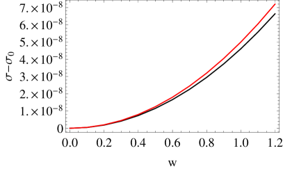
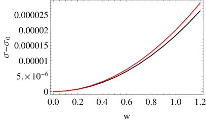
Figure 5: Enhancement of $\sigma_{\rm DC}$ at low $\rho$. We plot the subtracted $\sigma_{\rm DC}$ as a function of the noise strength $w$. The black line corresponds to the numerical simulation, while the red line to the analytic expression for small noise (3.17). The left panel shows the results for $\mu_{0}=0.005$, and the right one for $\mu_{0}=0.1$. The numerical results follow from averaging over 10 simulations on a grid of size $100\times 100$, with $L_{x}=20\pi$ and $k_{*}=1$.

In Fig. 6 we turn our attention to the case of large $\rho$, and again plot the subtracted conductivity as a function of the noise strength $w$. We present both the numerical results (black lines) and the analytic prediction of Eq. (3.23) (red lines). We consider systems with $\mu_{0}=10$, and $\mu_{0}=20$, which at $w=0$ correspond respectively to $\rho_{0}=37.897$, and $\rho_{0}=133.398$. The plots show a good agreement between analytic and numeric results, and confirm the prediction that disorder decreases the conductivity in the limit of large charge density.

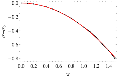
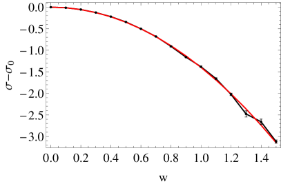
Figure 6: Decrease of $\sigma_{\rm DC}$ at large $\rho$ as a function of noise. We plot the subtracted $\sigma_{\rm DC}$ as a function of the noise strength $w$. The black line shows the numerical results, and the red line the prediction (3.23) for small noise. On the left panel we have set $\mu_{0}=10$, and on the right $\mu_{0}=20$. The numerical results follow from averaging over 10 realizations on a grid of size $100\times 100$, with $L_{x}=20\pi$ and $k_{*}=1$.

We now proceed to study the disordered conductivity for the whole range of the chemical potential, and in Figs. 7 and 8 we plot $\sigma_{\rm DC}$ versus $\mu_{0}$ for noisy chemical potentials of the form (2.12). First, in Fig. 7 we present the results of our simulations along a wide range of $\mu_{0}$ for four different values of the strength of noise: from $w=0$ (orange line) corresponding to the clean system, up to $w=3$ (blue line) which, when setting $k_{*}=1$ in the sum (2.12), corresponds to a noisy chemical potential whose maximum oscillations have amplitudes $\approx 70\%\,\mu_{0}$. Except for the low $\mu_{0}$ region, which we will resolve in Fig. 8, the plot shows that the noise has the effect of reducing the conductivity, and this effect increases with $\mu_{0}$. Notice however, that even for the strongest noise studied, the conductivity is still increasing towards higher $\mu_{0}$, and is always larger than the conformal value $\sigma_{\rm DC}=1$. Actually, one can see from Eq. (3.9) that $\sigma_{\rm DC}>1$ for any noise, and thus the system behaves always as a metal.

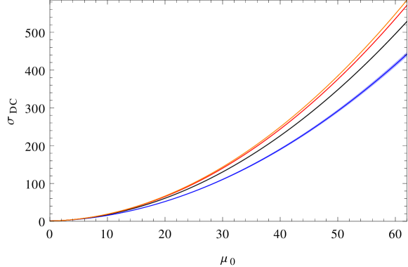
Figure 7: $\sigma_{\rm DC}$ versus $\mu_{0}$. The different lines correspond, from top to bottom, to noisy chemical potentials with $w=0,1,2,3$. The numerical results follow after averaging over 36 simulations on a grid of size $100\times 100$, with $L_{x}=20\pi$ and $k_{*}=1$. We plot with color bands the error of the average, which is only visible in the $w=3$ case.

We have shown above, when studying the weak disorder case, that an enhancement of $\sigma_{\rm DC}$ is observed in the small charge density limit. To examine more closely the effect of disorder at low values of $\mu_{0}$, and therefore resolve the leftmost region of the plot in Fig. 7, in Fig. 8 left we plot $\sigma_{\rm DC}$ for $w=3$, and compare it with the homogeneous result. We observe that for values of $\mu_{0}\lesssim 1$ the conductivity is slightly enhanced in presence of noise. To better illustrate this fact, and pinpoint the value of $\mu_{0}$ above which the noise stops enhancing the conductivity and starts decreasing it, on the right panel of Fig. 8 we plot the subtracted conductivity (i.e. the difference between the noisy and the homogeneous results). We observe that the maximum enhancement occurs at $\mu_{0}\approx 0.8$, and that the critical value at which the enhancement ceases is in the interval $(1.1,\,1.2)$ (see caption of Fig. 8).

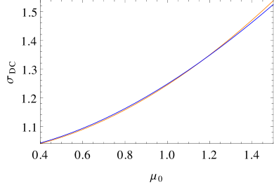
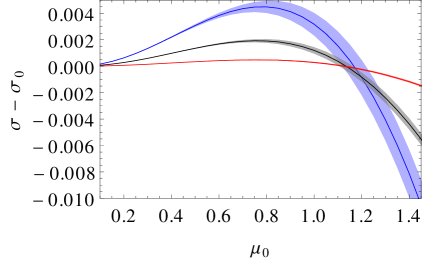
Figure 8: Evolution of $\sigma_{DC}$ versus $\mu_{0}$; comparison of the clean and noisy systems. On the left the orange line shows the clean case, and the blue line the noisy system with $w=3$. On the right we plot the difference between the clean and the noisy cases, $\sigma-\sigma_{0}$, versus $\mu_{0}$. The three lines correspond to $w=1,2,3$ (red, black, and blue respectively). The value of the chemical potential at which $\sigma-\sigma_{0}$ changes sign lies in the interval $(1.15,\,1.20)$ for $w=3$ and $(1.10,\,1.15)$ for $w=1,\,2$. We have averaged over $36$ simulations on a grid of size $100\times 100$, with $L_{x}=20\pi$ and $k_{*}=1$. The color bands correspond to the standard deviation.

It is not difficult to estimate that the change of sign in the right panel of Fig. 8 should occur at $\mu_{0}\approx 1$. Indeed from the expression (3.14) for the resistivity in the small charge limit one can see that the noisy correction proportional to $\tilde{w}^{2}$ changes sign at $\mu_{0}\approx 2/d^{2}=1$.

3.4.1 DC conductivity as a function of the charge density

In this section we will study how the DC conductivity behaves as a function of the charge density in presence of disorder. This analysis will allow us to compare the qualitative behavior of our system to that of semimetal graphene close to its charge neutrality point. Experimental results PhysRevLett.99.246803 show that the DC conductivity of clean enough graphene samples displays the following features: a nonzero minimal conductivity at vanishing charge density, a linear behavior $\sigma_{\rm DC}\propto\rho$ up to some critical charge $\rho_{*}$ that is sample dependent (namely, determined by the amount of impurities), and a sublinear behavior for larger values of the charge density.

In Sec. 3.3 we have computed a semi-analytical prediction for the evolution of $\sigma_{\rm DC}$ as a function of $\langle\rho\rangle$. We shall now present results following both from the purely numerical solution of the system, and the semi-analytical approach given by Eq. (3.24), compare them, and show their agreement. First, we will show numerical results for $\sigma_{\rm DC}$ at moderate noise, that is for a value of the strength of noise $w$ such that the chemical potential becomes very small at its minima, but neither $\mu(x)$ nor the charge density $\rho(x)$ ever become negative. Next, we will present the numerical results for $\sigma_{\rm DC}$ vs $\langle\rho\rangle$ for strong noise. This is a scenario in which the oscillations of the chemical potential are so large that regions of negative charge appear in the system, bringing the setup to a configuration resembling that of graphene near the Dirac point, when puddles of charge of different sign are expected to be present in the system Lucas:2015sya ; PhysRevLett.107.156601 .

In Fig. 9 we consider the case of moderate noise and plot the numerical results for $\sigma_{\rm DC}$ as a function of $\langle\rho\rangle$ for a fixed strength of noise $w=3$ (green line). For this value of $w$ the maximum oscillations of the chemical potential are of order 70% $\mu_{0}$, and both $\mu(x)$ and $\rho(x)$ stay positive for all $x$. One can observe that, as for a clean system, $\sigma_{\rm DC}$ is linear in $\langle\rho\rangle$ (except for very low values of $\langle\rho\rangle$). However, the slope is much lower than that of the clean system (blue dashed line), and agrees very well with that predicted in Eq. (3.31) above (black dashed line).

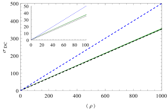
Figure 9: DC conductivity as function of the charge density. The blue dashed upper line corresponds to the clean case. The solid green line is the numerical simulation for the noisy case with $\omega=3$, and the green band shows the error of the average. The black dashed line corresponds to the analytic prediction (3.31). We have used a grid of size $100\times 100$, set $L_{x}=20\pi$, $k_{*}=1$, and averaged over 36 realizations.

Strong noise: We focus now on the scenario where the strength of noise is large enough for $\mu(x)$, and $\rho(x)$, to change sign repeatedly along the system. In Fig. 10 we present numerical results for $w=6$, and 8 (green and black solid lines respectively).

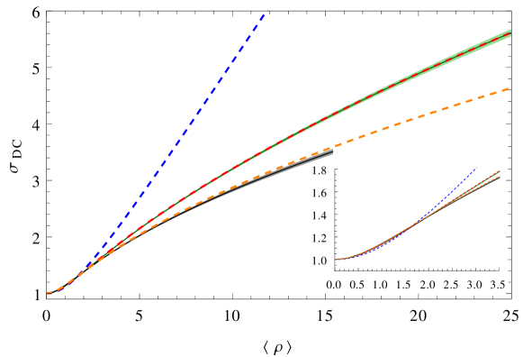
Figure 10: DC conductivity as function of the charge density. The blue dashed upper line corresponds to the clean case. The solid green, and solid black lines are the numerical data for $w=6$ and $w=8$ respectively. The dashed red line for $w=6$, and the dashed orange line for $w=8$ show the semi-analytical prediction of Eq. (3.24) after averaging over 1000 realizations. As before, shaded bands depict the error of the average. We have used a grid of size $120\times 120$, set $k_{*}=1$, $L_{x}=20\pi$, and averaged over 43 and 57 realizations for $w=6$ and $w=8$ respectively.

The numerical computation of $\sigma_{\rm DC}$ for these large values of $w$ becomes quite delicate, and as a consequence, the range of $\langle\rho\rangle$ where we can trust our results is significantly restricted with respect to the case of $w=3$ in Fig. 9. In particular, notice that for $w=8$ we have numerical results only up to $\langle\rho\rangle\approx 16$. We have studied the stability of our results against the lattice size in Fig. 14 in the appendix.

For large values of $w$ the analytic weak noise prediction (3.31) is not reliable, and we instead compare our numerics to the prediction (3.24) where all orders in $w$ are kept. First, it is remarkable how well our semi-analytical prediction works at $w=6$ (red dashed line) and $w=8$ (orange dashed line). Notice that the approximation that led us to that expression, which effectively neglects the effect of gradients along $x$, should become less reliable as one increases $w$, $\mu_{0}$, or both, and those gradients become larger. One indeed expects that for large enough $w$ and $\mu_{0}$, the effect of the gradients become important and our semi-analytical approach fail. A closer inspection of Fig. 10 reveals that for the case of $w=8$, at the largest values of $\langle\rho\rangle$ we have reached the numerical results fall slightly below the prediction of Eq. (3.24). This effect seems to be enhanced for the case $w=10$ we present in Fig. 15 of the appendix, although a more ambitious numerical study that would allow larger values of $w$ and $\langle\rho\rangle$ would be needed to settle the question. A decrease of $\sigma_{\rm DC}$ due to the $x$ dependent gradients is to be expected on general grounds, since gradients of the charge density result in a reduction of the diffusion constant Ryu:2011vq . Additionally, increasing $k_{*}$, thus reducing the correlation length of our noise (2.12), one also expects the effects of the gradients to become more important. However, we postpone a more thorough numerical study, including an analysis of the effect of $k_{*}$, to a future work where a more realistic two-dimensional noise, which would get us closer to the situation in graphene, will be implemented.

Finally, one readily notices that in Fig. 10, after a short region at very low $\langle\rho\rangle$ where they largely agree with the clean case (dashed blue line), the noisy conductivities become sublinear. To characterize this sublinear behavior, in Fig. 11 we examine closely the asymptotic behavior of $\sigma_{\rm DC}$ in the limits of small and large $\langle\rho\rangle$.

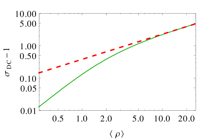
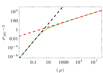
Figure 11: log-log plot of $\sigma_{\rm DC}$ versus $\langle\rho\rangle$. On the left we present our numerical data for $\sigma_{\rm DC}$ at $w=6$ featured in Fig. 10 (green solid line). The red dashed line depicts a linear fit to the $\langle\rho\rangle>15$ region, resulting in $\log_{10}(\sigma_{DC}-1)=0.78\,\log_{10}\langle\rho\rangle-0.42$. On the right we plot $\sigma_{\rm DC}$ computed from Eq. (3.24) with $w=8$ (green solid line), having set $k_{*}=1$ and $L_{x}=20\pi$. The black dashed line shows the linear fit $\log_{10}(\sigma_{DC}-1)=2.00\,\log_{10}\langle\rho\rangle-0.72$ in the region $\langle\rho\rangle<0.1$, while the red dashed line corresponds to the fit $\log_{10}(\sigma_{DC}-1)=0.53\,\log_{10}\langle\rho\rangle-0.01$ in the region $10^{5}\lesssim\langle\rho\rangle\lesssim 10^{8}$. We have averaged over 33 realization of the noise.

By employing the semi-analytical expression (3.24), we compute $\sigma_{\rm DC}$ for $w=8$ for a wide range of values of $\langle\rho\rangle$ (up to $\sim 10^{8}$). The resulting data is shown as the green solid line on the right panel of Fig. 11. Also in that plot we present logarithmic fits in the low (black dashed line) and high (red dashed line) charge regions. These fits reveal a quadratic growth $\sigma_{\rm DC}\propto\langle\rho\rangle^{2}$ in the small $\langle\rho\rangle$ region, and a sublinear trend $\sigma_{\rm DC}\propto\langle\rho\rangle^{0.53}$ as $\langle\rho\rangle$ becomes large. Notice that the result at small $\langle\rho\rangle$ agrees perfectly with the prediction (3.45) resulting from the strong noise analysis. Moreover, the behavior at large charge density is very close to that predicted in Eq. (3.43), pointing towards an asymptotic behavior $\sigma_{\rm DC}\propto\sqrt{\langle\rho\rangle}$. Finally, in Fig. 11 left we present a logarithmic fit of the numerical results for $w=6$. The fit is realized in the region of largest charge density available ($15\lesssim\langle\rho\rangle\lesssim 25$), where $\langle\rho\rangle$ is not large enough for the system to be properly in the large charge regime. Nevertheless, the data displays a clearly nonlinear behavior, with the fit resulting in a growth trend $\sigma_{\rm DC}\propto\langle\rho\rangle^{0.78}$. In view of these results it is worth mentioning that theoretical models of electric transport in graphene predict this sublinear behavior as a result of the presence of charged impurities in the system PhysRevLett.98.186806 ; PhysRevLett.107.156601 , with emphasis on this disorder creating puddles of charge of opposite sign.

3.4.2 Noisy DC at vanishing $\langle\rho\rangle$

We will finish this section by considering the case of a noisy chemical potential with vanishing spatial average of the form

$$\mu(x)=\hat{w}\,\sum_{k=k_{0}}^{k_{*}}\,\cos(k\,x+\delta_{k})\,,$$ (3.46)

which corresponds to Eq. (2.12) in the limit $\mu_{0}\to 0$, $w\to\infty$ with $\hat{w}\propto\mu_{0}\,w$ fixed. We will then be studying a system where the regions of positive and negative charge average to zero.

To find asymptotic expressions at low and high $\hat{w}$, we can again use Eq. (3.24). For low values of $\hat{w}$, expanding in $\hat{w}$ and using Eq. (A.33a), which gives $\rho(\mu)$ in the low charge limit, it is straightforward to check that the conductivity grows quadratically with $\hat{w}$:

$$\sigma_{DC}\approx 1+\frac{\hat{w}^{2}}{4}\Delta.$$ (3.47)

On the other hand, for high values of $\hat{w}$, the situation is analogous to the strong noise case at large $\langle\rho\rangle$. Zones of positive and negative charge are present in the system for any $\hat{w}$, and thus we can apply the analysis of Sec. 3.3 based on the existence of zeros of $\mu(x)$. Modifying suitably the definition of $\eta(x)$ as

$$\eta(x)=\sum_{k=k_{0}}^{k_{*}}\,\cos(k\,x+\delta_{k})\,,$$ (3.48)

and assigning to $\hat{w}$ the roll played by $\mu_{0}$ in that analysis, the asymptotic expression for the conductivity at large $\hat{w}$ is analogous to Eq. (3.41):

$$\sigma_{DC}\sim\frac{\hat{w}L_{x}}{7.083}\left<\frac{1}{\sum_{i}\frac{1}{|\eta^{\prime}(x_{i})|}}\right>_{\mathrm{noise}},$$ (3.49)

and thus, linear in $\hat{w}$.

In Fig. 12 we present both numerical and semi-analytical results for $\sigma_{\rm DC}(\hat{w})$. First, on the left panel we plot our numerical data (solid green line), and compare them with the result of the semi-analytical expression (3.24) (dashed red line). As it happens in Fig. 10 for the strongest noise there ($w=8$), our numerical results at the highest $\hat{w}$ available are slightly below the semi-analytical prediction, again showing a likely onset of the effects of the gradients along $x$ (which are neglected in the semi-analytical approximation). Next, in Fig. 12 right we study the asymptotic behavior of the semi-analytical result (solid green line) both in the small, and large $\hat{w}$ limits. We perform logarithmic fits in the small (black dashed line), and large (red dashed line) $\hat{w}$ region. The fits (see caption) confirm the expected quadratic behavior at small $\hat{w}$, and linear trend in the large $\hat{w}$ limit. In particular, for a system as that of Fig. 12, Eq. (3.47) gives $\log_{10}(\sigma_{DC}-1)=2\log_{10}\hat{w}+0.10$, while Eq. (3.49) using the same noise realizations of Fig. 12 results in $\log_{10}(\sigma_{DC}-1)=\log_{10}\hat{w}-0.03$. Notice the perfect agreement at small $\hat{w}$, while at large $\hat{w}$, as it happened in the last section for the large charge limit, we expect the semi-analytical data to eventually agree with the prediction in the asymptotic $\hat{w}\to\infty$ limit (we have observed how the fit of the data gets closer to the prediction (3.49) as larger $\hat{w}$ data points are included in the fit).

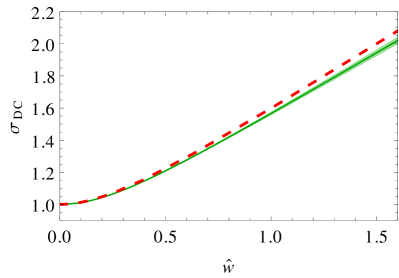
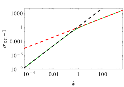
Figure 12: Evolution of $\sigma_{DC}$ versus $\hat{w}$. On the left we plot our numerical results (solid green line) after averaging over 22 realizations on a lattice $100\times 100$ and a noise with $k_{*}=1$ and $L_{x}=20\pi$. We also plot the error with shaded bands. The dashed red line shows the semi-analytical prediction of Eq. (3.24) after averaging over the same noise realizations. On the right we present a logarithmic plot of the same semi-analytical prediction in a broader range (solid green line). The black dashed line shows the linear fit $\log_{10}(\sigma_{DC}-1)=2.00\,\log_{10}\hat{w}+0.10$ in the region $\hat{w}<3\cdot 10^{-3}$, while the red dashed line corresponds to the fit $\log_{10}(\sigma_{DC}-1)=1.01\,\log_{10}\hat{w}-0.08$ in the region $50<\hat{w}<10^{4}$.

4 Spectral properties

In this section we consider a realization of disorder characterized by a power spectrum. Namely, a chemical potential of the form

$$\mu(x) = \mu_{0}+{\mu_{0}\over 25}\,w\,\sum_{k=k_{0}}^{k_{*}}\sqrt{S(k)}\,\cos(k\,x+\delta_{k})\,,$$ (4.1)

where

$$S(k)={1\over k^{2\alpha}}$$ (4.2)

is the power spectrum of our noise. Notice that the disordered chemical potential considered in previous sections corresponds to a flat spectrum with $\alpha=0$. As discussed in Arean:2014oaa , for a spectrum with $\alpha>0$ the typical length scale of the noise is of the order of the system size, and hence we will denote this case as correlated noise.

We will construct massive embeddings with a noisy chemical potential of the form (4.1) and analyze the power spectra of the observables of the system, namely the charge density $\rho(x)$, and the quark condensate $c(x)$. For a given input chemical potential with power spectrum $k^{-2\alpha}$ as above, we will compute the power spectra of the charge density $S_{\rho}(k)$, and the quark condensate $S_{c}(k)$, and study how they behave as functions of $\alpha$. Let us then define

$$S_{\rho}(k)={1\over k^{2\Gamma(\alpha)}}\,,\qquad S_{c}(k)={1\over k^{2\Delta(\alpha)}}$$ (4.3)

as the spectra of the charge density and quark condensate respectively.

In Arean:2013mta ; Arean:2014oaa , in the context of models of holographic superconductors, it was found a certain universal behavior for the spectra of the VEVs of the model as functions of the input power spectrum defining the chemical potential. In particular, for an input power spectrum $\leavevmode\nobreak\ k^{2\alpha}$ as above, the output power spectra (those of the VEVs) were of the form $\sim k^{2\alpha+d}$, with $d$ an integer coefficient different for each operator. This was interpreted as a kind of renormalization of small wave lengths in which higher harmonics of the VEVs of the corresponding operators are suppressed or enhanced, depending on the sign of the coefficient $d$ in the output power spectra.

In order to determine the power spectra of the charge density and quark condensate ($S_{\rho}$ and $S_{c}$), we construct massive embeddings characterized by a chemical potential of the form (4.1) for different values of $\alpha$. We keep fixed $m=0.5$, $\mu_{0}=1$, and $w=1$.. From the asymptotic behavior of the embedding fields $\chi$ and $\phi$ we can read $\rho$ and $c$, and determine their power spectra, namely $\Gamma$ and $\Delta$.

Figure 13: Power spectrum of the VEVs. Black dots correspond to the numerical result averaging over 35 realizations on a lattice of size $N_{z}=40$, $N_{x}=100$, for a system with $L_{x}=3\pi/2$, and $k_{*}=62.7$ (corresponding to 47 modes in the sum (4.1)). On the left, for the charge density we plot $\Gamma$ versus $\alpha$, and the red line stands for the fit $\Gamma=1.00\alpha-1.00$. On the right, for the quark condensate, we plot $\Delta$ versus $\alpha$, the red line shows the fit $\Delta=1.01\alpha+2.99$.

We observe that they are very well approximated by

$$\Gamma\approx\alpha-1\,,\qquad\Delta\approx\alpha+3\,.$$ (4.4)

Notice that the power spectrum renormalization of the charge density agrees with that found in Arean:2013mta ; Arean:2014oaa , and implies that higher harmonics are enhanced with respect to the input power spectrum. The opposite effect is observed for the quark condensate; the power spectrum renormalization we observe implies that the higher harmonics are suppressed, and $c(x)$ is then smoothed out with respect to the input $\mu(x)$. To illustrate these facts, in Fig. 16 of App. C we plot the result of a simulation for an embedding with correlated noise.

5 Conclusions and outlook

In this note we have presented a holographic model of (2+1)-dimensional charged matter with a disordered chemical potential. The model is built upon a D3/D5 intersection at finite temperature and charge density, and the chemical potential consists of random fluctuations about a nonzero baseline value. We have worked in the probe limit where the setup reduces to inhomogeneous embeddings of a D5-brane in a neutral black hole background. The construction of these embeddings has allowed us to study, both numerically and analytically, how the disorder affects the quark condensate and the charge density. In particular, we have found that in the regime of moderate to large charge density, this quantity is enhanced by disorder, while the quark condensate is largely unaffected.

Arguably the main outcome of this work is the study of the DC conductivity for a top-down holographic model of charged matter in the presence of disorder. In the spirit of the membrane paradigm, the DC conductivity of our model can be expressed purely in terms of horizon data of the background functions (those characterizing the embedding), and hence we could compute the conductivity of our disordered setup without having to solve for the fluctuations. In the limit of weak disorder we obtained analytic expressions showing that disorder enhances the conductivity at very small charge density, while decreasing it in the opposite regime, i.e. large charge density. Numerical simulations in agreement with the analytic predictions confirmed this behavior. We have also studied the behavior of the DC conductivity as a function of the charge density, both through numerical simulations and analytic approximations. At weak noise the DC conductivity scales linearly with the charge density, with a slope that decreases as the strength of noise is increased, and which is always lower than that of the clean system. At strong noise, a sublinear trend is observed in our numerical simulations. Moreover, a careful analysis of our semi-analytical approximations confirmed that $\sigma_{\rm DC}$ becomes a sublinear function of the spatial average of the charge density as this becomes large. This onset of sublinearities resembles that found in some regimes of graphene, a context in which it was attributed to the effects of disorder PhysRevLett.98.186806 ; PhysRevLett.107.156601 .

In a slightly tangential direction, we have also studied the effects of a noisy chemical potential characterized by a Fourier power spectrum. This noise is correlated along distances of the order of the system size, and thus we refer to it as ‘correlated noise’. In this scenario we have analyzed the spectral properties of the VEVs of the system: charge density and quark condensate, observing what amounts to a spectral renormalization of sorts. For an input Fourier power spectrum of the chemical potential of the form $1/k^{2\alpha}$, the output power spectra of the VEVs are given by $1/k^{2\alpha+d}$, with $d\approx-2$ for the charge density, and $d\approx 6$ for the quark condensate. Therefore, the higher wave numbers are enhanced in the spectrum of the charge density, which is then more irregular than the chemical potential; while the opposite occurs for the quark condensate: the higher wave numbers are suppressed in the spectrum and the quark condensate is a smoother function of the space direction $x$. This phenomenon was already observed in Arean:2013mta ; Arean:2014oaa for holographic models of superconductivity, and it deserves further study, specially in relation with the universal response of the AdS geometry to time dependent sources found in Buchel:2013gba .

The analysis we have presented has revealed the D3/D5 intersection as a reasonably tractable top-down model of disordered matter with the potential to reproduce behaviors observed in strongly coupled Condensed Matter systems. Our results motivate a further exploration of disordered brane models, and there are several directions in which we plan to make progress in the future. First, the most obvious step would be to extend our D3/D5 model to the case where the chemical potential is disordered along both spatial directions. Impurities in two-dimensional systems like graphene or thin superconducting films are randomly distributed along the two spatial dimensions (although some correlation might still be present, see PhysRevLett.107.156601 ), and hence considering two-dimensional disorder is the natural procedure. Moreover, according to the Harris criterion Harris:1974zz , that generalizes the standard power-counting criterion to random couplings, a chemical potential with random spatial inhomogeneities in 2 dimensions amounts to the introduction of marginally relevant quenched disorder. Instead, as explained in Garcia-Garcia:2015crx , the present case where the chemical potential is disordered only along one direction corresponds to a relevant noise. This fact would make an eventual extension of the present model beyond the probe limit both very interesting, and potentially very challenging. In addition to changing the dimensionality of disorder, for applications to graphene near the charge neutrality point, it would be interesting to investigate further the case of strong noise where the charge density changes sign along the system. While this would be problematic in a scenario of massive embeddings, for which the topology could change when the charge density vanish, we have showed that it works for massless embeddings. In this context it would be interesting to extend our results for the DC conductivity to larger values of the charge density and the noise strength.

Another interesting possibility would be to consider more sophisticated models where one could tune the total charge density, and that of the impurities separately. A suitable framework could be that of Sen’s tachyonic action for an overlapping brane-antibrane pair Sen:2003tm , which was used in Arean:2015wea to model superfluid phase transitions. One could deform the finite density configuration of Arean:2015wea by switching on a disordered source for the scalar operator dual to the tachyon which would be akin to a doping parameter. Finally, the definitive step forward would be to account for the backreaction of the flavor branes on the geometry, working in the Veneziano limit in which both the number of color branes, $N_{c}$, and flavor branes, $N_{f}$, are large, but $x=N_{f}/N_{c}$ is kept fixed. This limit, which is more tractable when the flavor branes are smeared along their orthogonal directions Bigazzi:2005md ; Nunez:2010sf , would allow us to study the RG flow of the dual disordered theory, and hopefully to characterize its ground state. Additionally, the whole set of transport coefficients would be accessible (recall that heat transport is dual to metric fluctuations, and hence inaccessible in the probe limit), and the computed results reliable down to very low temperature. Solutions dual to brane intersections in the Veneziano limit and with a nonzero density of (2+1)-dimensional flavor degrees of freedom have been constructed in Faedo:2015urf . Interestingly, their IR geometry is a hyperscaling violating Lifshitz-like geometry. A compelling and challenging, problem is then to introduce disorder in these solutions, again through the chemical potential, and study the fate of the IR fixed point.

Appendix A The homogeneous case

In this appendix we shall briefly review some interesting results of the homogeneous D3/D5 system that are useful for the analysis in this paper.

For an embedding where $\chi$ and $\phi$ depend only on $z$ the DBI action (2.5) takes the form

$${{\cal S}\over N_{f}\,T_{D5}\,L^{6}}\equiv\bar{\cal S}=-\int dt\,d^{2}x\,dz\,d\Omega_{2}\,{f\over z^{4}}\,\sqrt{h\,(1-\chi^{2})\,\left[1-\chi^{2}+z^{2}\chi^{\prime 2}-\frac{z^{4}(1-\chi^{2})}{f^{2}}h\,\phi^{\prime 2}\right]}\,.$$ (A.1)

In this action, $\phi$ is a cyclic coordinate. Thus, its conjugate generalized momentum is a conserved quantity,

$$d=\frac{\delta\bar{\cal S}}{\delta\phi^{\prime}}=\frac{h^{\frac{3}{2}}}{f}\frac{(1-\chi^{2})^{\frac{3}{2}}\phi^{\prime}}{\sqrt{1-\chi^{2}+z^{2}\chi^{\prime 2}-\frac{z^{4}(1-\chi^{2})}{f^{2}}h\,\phi^{\prime 2}}}\,.$$ (A.2)

Taking into account the asymptotic behavior of $\phi$ and $\chi$ given in Eqs. (2.8), one finds that $d$ is exactly the charge density $\rho$.

In order to obtain the equation of motion of $\chi$ it is useful to compute the Legendre transformed action with respect to $\phi^{\prime}$

$$\hat{\cal S}=\bar{\cal S}-\int dt\,d^{2}x\,dz\,d\Omega_{2}\,\,\rho\,\phi^{\prime},$$ (A.3)

which expressed in terms of the variables $\chi$, $\chi^{\prime}$ and $\rho$ reads

$$\hat{\cal S}=-\int dt\,d^{2}x\,dz\,d\Omega_{2}\,\frac{f\sqrt{h(1-\chi^{2})(1-\chi^{2}+z^{2}\chi^{\prime 2})}}{z^{4}}\,\sqrt{1+\frac{\rho^{2}z^{4}}{h^{2}(1-\chi^{2})^{2}}}\,,$$ (A.4)

and leads to the equation of motion

$$-\frac{d}{dz}\left[\frac{f\chi^{\prime}\sqrt{h(1-\chi^{2})}}{z^{2}\sqrt{1-\chi^{2}+z^{2}\chi^{\prime 2}}}\sqrt{1+\frac{\rho^{2}z^{4}}{h^{2}(1-\chi^{2})^{2}}}\right]$$

$$=\frac{f\sqrt{h}\chi}{z^{4}\sqrt{(1-\chi^{2})(1-\chi^{2}+z^{2}\chi^{\prime 2})}}\sqrt{1+\frac{\rho^{2}z^{4}}{h^{2}(1-\chi^{2})^{2}}}\left[2-2\chi^{2}+z^{2}\chi^{\prime 2}-\frac{2\rho^{2}z^{4}(1-\chi^{2}+z^{2}\chi^{\prime 2})}{\rho^{2}z^{4}+h^{2}(1-\chi^{2})^{2}}\right]\,.$$ (A.5)

Recall that when integrating this equation one must impose regularity at the horizon, which in view of the IR expansions (2.11) implies $\chi^{\prime}(1)=0$. This condition fixes one of the two constants of integration and therefore the quark mass $m$ and the quark condensate $c$ are not independent anymore. Only numerical solutions of Eq. (A.5) are known, and thus one cannot express $c$ as an analytic function of $\mu$. However, as we will see in the next two sections, semi-analytical expressions can be obtained in the small and large charge limits.

A.1 Small charge limit

For $\rho\to 0$, Eq. (A.5) can be expanded in powers of $\rho^{2}$ as

$$-\frac{d}{dz}\left\{\frac{f\chi^{\prime}\sqrt{h(1-\chi^{2})}}{z^{2}\sqrt{1-\chi^{2}+z^{2}\chi^{\prime 2}}}\left[1+\frac{\rho^{2}z^{4}}{2h^{2}(1-\chi^{2})^{2}}\right]\right\}$$

$$=\frac{f\sqrt{h}\chi}{z^{4}\sqrt{(1-\chi^{2})(1-\chi^{2}+z^{2}\chi^{\prime 2})}}\left[2-2\chi^{2}+z^{2}\chi^{\prime 2}-\rho^{2}z^{4}\frac{2-2\chi^{2}+3z^{2}\chi^{\prime 2}}{2h^{2}(1-\chi^{2})^{2}}\right]+O(\rho^{4})\,.$$ (A.6)

This equation allows us to solve for $\chi$ as a power series in $\rho^{2}$. Let us define

$$\chi(z)=\chi_{0}(z)+\rho^{2}\chi_{1}(z)+O(\rho^{4})\,,$$ (A.7)

and use the asymptotic UV expansion (2.8b) to express the quark condensate $c$ as

$$c=\frac{1}{2}\chi^{\prime\prime}_{0}(0)+\frac{\rho^{2}}{2}\chi^{\prime\prime}_{1}(0)+O(\rho^{4})\,.$$ (A.8)

Next, to solve for the functions $\chi_{n}$ we substitute Eq. (A.7) in the equation of motion (A.6). The resulting equation can be solved order by order in $\rho^{2}$. At order zero we obtain the following differential equation for $\chi_{0}(z)$

$$-\frac{d}{dz}\left[\frac{f\chi_{0}^{\prime}\sqrt{h(1-\chi_{0}^{2})}}{z^{2}\sqrt{1-\chi_{0}^{2}+z^{2}\chi_{0}^{\prime 2}}}\right]=\frac{f\sqrt{h}\chi_{0}}{z^{4}\sqrt{(1-\chi_{0}^{2})(1-\chi_{0}^{2}+z^{2}\chi_{0}^{\prime 2})}}\left[2-2\chi_{0}^{2}+z^{2}\chi_{0}^{\prime 2}\right]\,,$$ (A.9)

which is nothing else than the equation of motion for $\chi(z)$ at zero charge density. The boundary conditions for a black hole embedding with fixed mass are $\chi_{0}^{\prime}(0)=m$ in the UV, where $m$ is the mass of the quarks, and $\chi_{0}^{\prime}(1)=0$ at the horizon. Solutions with these boundary conditions exist only when $m\lesssim 1.41$, while for $m>1.41$ only Minkowski embeddings, for which the brane never reaches the black hole horizon, exist Kobayashi:2006sb ; Evans:2008nf . We will restrict the analysis to the case $m<1.41$, which is also the range we consider in Sec. 2.5. Once the solution for $\chi_{0}$ has been found, one can iteratively find the equations for $\chi_{n}$ with $n\geq 1$, and solve them with the boundary conditions $\chi_{n}^{\prime}(0)=\chi_{n}^{\prime}(1)=0$. The equation for $\chi_{1}(z)$, which determines the coefficient of the $\rho^{2}$ scaling of $c$ in Eq. (A.8), takes the form

$$g_{2}\chi_{1}^{\prime\prime}+\frac{dg_{2}}{dz}\chi_{1}^{\prime}+\left[\frac{dg_{1}}{dz}+g_{0}\right]\chi_{1}+\left[\frac{dg_{-1}}{dz}+g_{-2}\right]=0\,,$$ (A.10)

where the functions $g_{i}$ are defined as

$$g_{1}=-\frac{f\sqrt{h}\chi_{0}\chi_{0}^{\prime 3}}{\sqrt{1-\chi_{0}^{2}}\left(1-\chi_{0}^{2}+z^{2}\chi_{0}^{\prime 2}\right)^{\frac{3}{2}}}\,,\quad g_{2}=\frac{f\sqrt{h}(1-\chi_{0}^{2})^{\frac{3}{2}}}{z^{2}(1-\chi_{0}^{2}+z^{2}\chi_{0}^{2})^{\frac{3}{2}}}\,,$$

$$g_{0}=\frac{f\sqrt{h}\left[z^{4}\chi_{0}^{\prime 4}+3z^{2}\chi_{0}^{\prime 2}(1-\chi_{0}^{2})^{2}+2(1-\chi_{0}^{2})^{3}\right]}{z^{4}\left(1-\chi_{0}^{2}\right)^{\frac{3}{2}}\left(1-\chi_{0}^{2}+z^{2}\chi_{0}^{\prime 2}\right)^{\frac{3}{2}}}\,,$$

$$g_{-1}=\frac{fz^{2}\chi_{0}^{\prime}}{2h^{\frac{3}{2}}(1-\chi_{0}^{2})^{\frac{3}{2}}\sqrt{1-\chi_{0}^{2}+z^{2}\chi_{0}^{\prime 2}}}\,,\quad g_{-2}=-\frac{f\chi_{0}\left(2-2\chi_{0}^{2}+3z^{2}\chi_{0}^{\prime 2}\right)}{2h^{\frac{3}{2}}(1-\chi_{0}^{2})^{\frac{5}{2}}\sqrt{1-\chi_{0}^{2}+z^{2}\chi_{0}^{\prime 2}}}\,.$$ (A.11)

In order to express $c$ as a function of the chemical potential we need to determine the dependence of $\rho$ on $\mu$. The chemical potential can be expressed as

$$\mu=-\int_{0}^{1}dz\,\phi^{\prime}\,,$$ (A.12)

where we have taken into account that $\phi(1)=0$, and $\phi(0)=\mu$. Since $\phi^{\prime}(z)$ as function of $\rho$ and $\chi(z)$ is

$$\phi^{\prime}=-\frac{\delta\hat{\cal S}}{\delta\rho}\,,$$ (A.13)

one finds

$$\mu=\rho\int_{0}^{1}dz\,\frac{f\sqrt{1-\chi^{2}+z^{2}\chi^{\prime 2}}}{\sqrt{h(1-\chi^{2})[h^{2}(1-\chi^{2})^{2}+\rho^{2}z^{4}]}}\,.$$ (A.14)

The limit $\rho\to 0$ is easily found using Eq. (A.7),

$$\mu=\rho\int_{0}^{1}dz\,\frac{f\sqrt{1-\chi_{0}^{2}+z^{2}\chi_{0}^{\prime 2}}}{h^{\frac{3}{2}}(1-\chi_{0}^{2})^{\frac{3}{2}}}\left[1+O(\rho^{2})\right]\,.$$ (A.15)

Taking into account Eq. (A.8), we can express $c$ as function of $\mu$ for a fixed mass and $\mu\to 0$,

$$c=\frac{1}{2}\chi^{\prime\prime}_{0}(0)+\frac{\chi^{\prime\prime}_{1}(0)}{2\left[\int_{0}^{1}dz\,\frac{f\sqrt{1-\chi_{0}^{2}+z^{2}\chi_{0}^{\prime 2}}}{h^{\frac{3}{2}}(1-\chi_{0}^{2})^{\frac{3}{2}}}\right]^{2}}\,\mu^{2}+O(\mu^{4})\,.$$ (A.16)

Therefore, we see that at small enough $\mu$, the quark condensate scales quadratically with the chemical potential. This is confirmed by the numerical analysis shown in Fig. 4 where we considered an embedding with $m=0.5$. In Eq. (2.16a) we show the explicit form of Eq. (A.16), after numerically solving for $\chi_{0}$ and $\chi_{1}$ from Eqs. (A.9, A.10) for an embedding with $m=0.5$. The fit to the numerical data at low $\rho$ presented in Fig. 4 agrees very well with the prediction of Eq. (2.16a).

A.2 Large charge limit

The limit $\rho\to\infty$ can be analyzed in a similar way. However, there are some differences as Eq. (A.5) depends on $\rho^{2}\,z^{4}$, and thus there is always a neighborhood of $z=0$, where $\rho^{2}z^{4}$ stays finite in the limit $\rho\to\infty$. This makes $z=0$ a special point. If one tries to expand $\chi(z)=\chi_{0}(z)+\chi_{1}(z)\rho^{-1}+O\left(\rho^{-2}\right)$, nontrivial solutions to the resulting equations cannot satisfy $\chi^{\prime}(1)=0$ and $\chi(0)=0$ simultaneously. To address this problem we perform the change of variables $s=\sqrt{\rho}\,z$, and $\bar{\chi}=\sqrt{\rho}\,\chi$. The resulting equation can be solved perturbatively with the desired boundary conditions as we now see. The expansion of the equation after the change of variables in powers of $\rho^{-1}$ is

$$-\frac{d}{ds}\left\{\frac{\sqrt{1+s^{4}}\bar{\chi}^{\prime}}{s^{2}}-\frac{\left[(1+s^{4})\bar{\chi}^{\prime 2}-2s^{2}\bar{\chi}^{2}\right]\bar{\chi}^{\prime}}{2\rho\sqrt{1+s^{4}}}\right\}=\frac{2\bar{\chi}}{s^{4}\sqrt{1+s^{4}}}$$

$$-\frac{\left[2\bar{\chi}^{2}+s^{2}(1+s^{4})\bar{\chi}^{\prime 2}\right]\bar{\chi}}{\rho(1+s^{4})^{\frac{3}{2}}}+O(\rho^{-2}),$$ (A.17)

with the boundary conditions

$$\bar{\chi}^{\prime}(0)=m,$$

$$\bar{\chi}^{\prime}\left(\sqrt{\rho}\right)=0.$$ (A.18)

Eq. (A.17) can be solved in powers of $\rho^{-1}$, hence we expand

$$\bar{\chi}(s)=\bar{\chi}_{0}(s)+\bar{\chi}_{1}(s)\rho^{-1}+O(\rho^{-2})\,.$$ (A.19)

Inserting this expansion in Eq. (A.17), we find an equation for every $\bar{\chi}_{n}$ that can be solved iteratively. In terms of the original fields and variables we can write

$$\chi(z)=\frac{1}{\sqrt{\rho}}\left[\bar{\chi}_{0}\left(\sqrt{\rho}z\right)+\bar{\chi}_{1}\left(\sqrt{\rho}z\right)\rho^{-1}+O\left(\rho^{-2}\right)\right]\,,$$ (A.20)

which leads to the following expression for $c$ at large $\rho$,

$$c=\frac{\sqrt{\rho}}{2}\,\bar{\chi}^{\prime\prime}_{0}(0)+\frac{1}{2\sqrt{\rho}}\bar{\chi}^{\prime\prime}_{1}(0)+O\left(\rho^{-\frac{3}{2}}\right).$$ (A.21)

The equation determining $\bar{\chi}_{0}$ reads

$$s^{2}(1+s^{4})\,\bar{\chi}_{0}^{\prime\prime}-2s\,\bar{\chi}_{0}^{\prime}+2\bar{\chi}_{0}=0\,.$$ (A.22)

We are interested in solutions satisfying $\bar{\chi}^{\prime}_{0}(0)=m$, and $\displaystyle\lim_{s\to\infty}\bar{\chi}_{0}(s)<\infty$. They are given by

$$\bar{\chi}^{\prime}_{0}(s)=m\,s+m\,\frac{1+i}{2}\frac{s}{K(-1)}\,F\left(i\,\mathrm{arcsinh}\left(\frac{1+i}{\sqrt{2}}\,s\right),-1\right)\,,$$ (A.23)

where $F(\phi,n)$ is the elliptic integral of the first kind, and $K(n)$ is the complete elliptic integral of the first kind. Plugging this solution into Eq. (A.21) we obtain

$$c=-\frac{m}{\sqrt{2}K(-1)}\sqrt{\rho}+O\left(\rho^{-\frac{1}{2}}\right).$$ (A.24)

Finally to write $c$ as a function of $\mu$, we use (A.20) in Eq. (A.14) and arrive to

$$\mu=\rho\int_{0}^{1}dz\,\frac{f}{\sqrt{h(h^{2}+\rho^{2}z^{4})}}\left[1+O(\rho^{-1})\right].$$ (A.25)

This integral is solved in Eq. (A.32) below (for massless embeddings). Here, we anticipate the asymptotic behavior (A.33b) when $\rho\to\infty$, and write

$$\mu={\Gamma({1\over 4})\,\Gamma({5\over 4})\over\sqrt{\pi}}\,\sqrt{\rho}+O(\rho^{0})\,.$$ (A.26)

Combining this with Eq. (A.24) we finally arrive to the following expression for $c$ as a function of $\mu$ in the $\mu\to\infty$ limit

$$c=\frac{\sqrt{\pi}}{\sqrt{2}\,\,\Gamma\left(\frac{1}{4}\right)\Gamma\left(\frac{5}{4}\right)K(-1)}\,m\,\mu+O(\mu^{0})\,,$$ (A.27)

which for the case $m=0.5$ results in the expression (2.16b), which agrees reasonably well with the fit to the numerical data in Fig. 4.

A.3 Massless embeddings

In the following we will restrict the analysis to the massless homogeneous embedding where $\chi$ is identically zero, and $\phi$ is a function of $z$ only. In this case, the DBI action (A.1) simplifies further to

$$\bar{\cal S}=-\int dt\,d^{2}x\,dz\,d\Omega_{2}\,f\,z^{-4}\,\sqrt{h\left(1-{z^{4}\over f^{2}}\,h\,\phi^{\prime 2}\right)}\,,$$ (A.28)

and Eq. (A.2) results in the following expression for the charge density

$$\rho={h^{3\over 2}\over f}\,{\phi^{\prime}\over\sqrt{1-{z^{4}\over f^{2}}\,h\,\phi^{\prime 2}}}\,.$$ (A.29)

It is then straightforward to solve for $\phi^{\prime}$ in terms of $\rho$, which allows us to express the chemical potential as the following integral

$$\mu =-\int_{0}^{1}dz\,\phi^{\prime}$$

$$=\rho\,\int_{0}^{1}dz\,{f\over\sqrt{h\left(z^{4}\,\rho^{2}+h^{2}\right)}}\,,$$ (A.30)

and after applying the following change of variables

$$z^{2}={2\over u^{2}+\sqrt{u^{4}-4}}\,,$$ (A.31)

the integral can be evaluated analytically as

$$\mu = \int_{\sqrt{2}}^{\infty}du\,{\rho\over\sqrt{\rho^{2}+u^{4}}}$$ (A.32)

$$= {\rho\over\sqrt{2}}\,_{1}F_{2}\left({1\over 4},{1\over 2},{5\over 4};-{\rho^{2}\over 4}\right)\,,$$

where ${}_{1}F_{2}$ is the hypergeometric function. This hypergeometric function can be easily expanded in powers of $\rho$ both in the large and small $\rho$ limits, resulting in

$$\mu={\rho\over\sqrt{2}}+O(\rho^{3})\,;\qquad(\rho\ll 1)\,,$$ (A.33a)

$$\mu={\Gamma({1\over 4})\,\Gamma({5\over 4})\over\sqrt{\pi}}\,\sqrt{\rho}-{4\sqrt{2}\,\Gamma({5\over 4})\over\Gamma({1\over 4})}+O(\rho^{-2})\,;\qquad(\rho\gg 1)\,,$$ (A.33b)

It will be useful to solve for $\rho$ instead,

$$\rho\approx\sqrt{2}\mu\,;\qquad(\rho\ll 1)\,,$$ (A.34a)

$$\rho\approx 0.291\mu^{2}+0.823\mu+0.58\,;\qquad(\rho\gg 1)\,.$$ (A.34b)

A.3.1 DC Conductivity

We shall now turn our attention to the DC conductivity, which in Eq. (3.9) was expressed in terms of the behavior of $\phi$ at the horizon. For an homogeneous embedding, that equation reduces to

$$\sigma_{\rm DC}={1\over\sqrt{1-(a^{(2)})^{2}/2}}\,,$$ (A.35)

where $a^{(2)}$, which is defined through the IR expansion (2.11a), is now independent of $x$, and using (A.29) can be easily expressed in terms of $\rho$ as

$$a^{(2)}=\pm{\sqrt{2}\rho\over\sqrt{4+\rho^{2}}}\,.$$ (A.36)

Finally one can write the DC conductivity in terms of the charge density as

$$\sigma_{\rm DC}={1\over 2}\,\sqrt{4+\rho^{2}}\,.$$ (A.37)

It is illustrative to recall both the large and small $\rho$ limits of this result

$$\sigma_{\rm DC}=1+{\rho^{2}\over 8}+O(\rho^{4})\;;\quad(\rho\sim 0)\,,$$ (A.38)

$$\sigma_{\rm DC}={\rho\over 2}+O(1/\rho)\;;\quad(\rho\to\infty)\,.$$ (A.39)

Appendix B Numerical coda

In this appendix we present additional numerical results for the study of the dependence of $\sigma_{\rm DC}$ on the charge density performed in Sec. 3.4.1.

First, in order to assert the reliability of the numerical simulations generating Figs. 9 and 10 we study the stability of the value of $\sigma_{\rm DC}$ against the lattice size. In Fig 14 left, we plot $\sigma_{\rm DC}$ versus $\langle\rho\rangle$ at $w=3$ for lattices of size $60\times 60$, $80\times 80$, $100\times 100$ and $120\times 120$. One can observe that for lattices of size $100\times 100$ and larger the results have converged and become stable against the increase of lattice size.

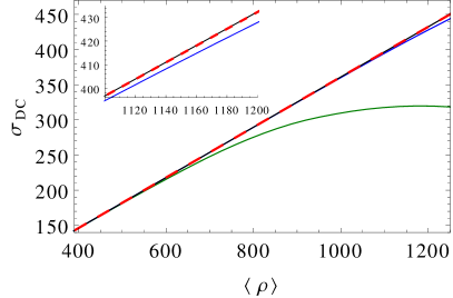
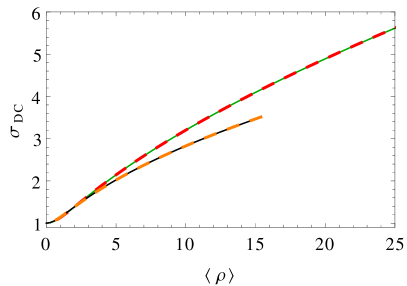
Figure 14: DC conductivity versus charge density. On the left we present data at $w=3$ for lattices of size $60\times 60$ (green solid line), $80\times 80$ (blue solid line), $100\times 100$ (red dashed line) and $120\times 120$ (black solid line). We have set $L_{x}=20\pi$, $k_{*}=1$, and averaged over 25 realizations. On the right we plot the results for lattices of size $100\times 100$ (dashed lines) and $120\times 120$ (solid lines) at strong noise: $w=6$ (green and red lines) and $w=8$ (black and orange lines). We have set $L_{x}=20\pi$, $k_{*}=1$, and averaged over 43 and 57 realizations for $w=6$ and $w=8$ respectively.

On the right panel of Fig. 14 we perform a similar exercise for $w=6$ (green and red lines), and $w=8$ (black and orange lines). In this case we just compare lattices of size $100\times 100$, and $120\times 120$. It becomes clear that for the ranges of $\langle\rho\rangle$ under study the results have converged too.

We close this appendix by extending the analysis in Fig. 10 to the case of a stronger noise with $w=10$. In Fig. 15 we plot our numerical result for $\sigma_{\rm DC}$ vs $\langle\rho\rangle$ (green solid line), and compare it to the semi-analytical prediction (3.24) (red dashed line). Although for this noise strength our numerics do not reach large values of the charge density, this result seems to confirm the observation made below Fig. 10 that for $w=8$ and higher, the numerical results fall slightly below the semi-analytical prediction for large enough $\langle\rho\rangle$.

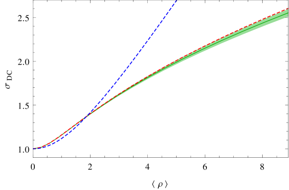
Figure 15: DC conductivity versus charge density at $w=10$ (green solid line). The red dashed line shows the prediction of Eq. (3.24) after averaging over 1000 realizations, and the blue dashed line the results for the clean system. We have used a grid of size $120\times 120$, set $k_{*}=1$, $L_{x}=20\pi$, and averaged over $30$ realizations. The shaded bands depict the error of the average.

Appendix C Embeddings with correlated noise

In this appendix we show the result of one simulation for the massive embeddings with correlated noise (4.1) considered in Sec. 4. In Fig. 16 we plot the input chemical potential $\mu(x)$, together with the output charge density $\rho(x)$, and quark condensate $c(x)$. These plots illustrate neatly the fact that while the charge density is roughened as a consequence of the enhancement of the higher wave numbers in the sum (4.1), the quark condensate is smoothed out due to the suppression of those same higher modes.

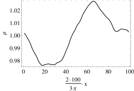
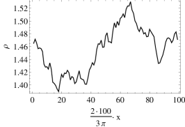
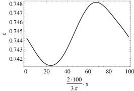
Figure 16: Massive embedding. The three panels display, from left to right, the chemical potential $\mu(x)$, the charge density $\rho(x)$, and the quark condensate $c(x)$ for a simulation with $\mu_{0}=1$, $m=0.5$, $w=1$, $\alpha=2$, $L_{x}=3\pi/2$, and $k_{*}=62.7$ (corresponding to 47 modes) on a lattice of size $N_{z}=40$, $N_{x}=100$.

References

- (1) S. H. Pan, J. O’Neal, R. Badzey, C. Chamon, H. Ding, J. Engelbrecht, Z. Wang and et al., Microscopic electronic inhomogeneity in the high-tc superconductor bi2sr2cacu2o8+x, Nature 413 (Sep, 2001) 282–285.
- (2) C. Renner, G. Aeppli, B. Kim, Y.-A. Soh and S. Cheong, Atomic-scale images of charge ordering in a mixed-valence manganite, Nature 416 (Apr, 2002) 518–521.
- (3) Y.-W. Tan, Y. Zhang, K. Bolotin, Y. Zhao, S. Adam, E. H. Hwang, S. Das Sarma, H. L. Stormer and P. Kim, Measurement of scattering rate and minimum conductivity in graphene, Phys. Rev. Lett. 99 (Dec, 2007) 246803.
- (4) E. H. Hwang, S. Adam and S. D. Sarma, Carrier transport in two-dimensional graphene layers, Phys. Rev. Lett. 98 (May, 2007) 186806.
- (5) A. Weinrib and B. I. Halperin, Critical phenomena in systems with long-range-correlated quenched disorder, Phys. Rev. B 27 (Jan, 1983) 413–427.
- (6) T. Vojta, Rare region effects at classical, quantum and nonequilibrium phase transitions, Journal of Physics A: Mathematical and General 39 (2006), no. 22 R143.
- (7) S. A. Hartnoll and J. E. Santos, Disordered horizons: Holography of randomly disordered fixed points, Phys. Rev. Lett. 112 (2014) 231601 [1402.0872].
- (8) A. M. Garcia-Garcia and B. Loureiro, Marginal and Irrelevant Disorder in Einstein-Maxwell backgrounds, Phys. Rev. D93 (2016), no. 6 065025 [1512.00194].
- (9) D. Arean, A. Farahi, L. A. Pando Zayas, I. S. Landea and A. Scardicchio, Holographic p-wave Superconductor with Disorder, JHEP 07 (2015) 046 [1407.7526].
- (10) D. Arean, A. Farahi, L. A. Pando Zayas, I. S. Landea and A. Scardicchio, Holographic superconductor with disorder, Phys. Rev. D89 (2014), no. 10 106003 [1308.1920].
- (11) A. Lucas, S. Sachdev and K. Schalm, Scale-invariant hyperscaling-violating holographic theories and the resistivity of strange metals with random-field disorder, Phys. Rev. D89 (2014), no. 6 066018 [1401.7993].
- (12) A. Donos and J. P. Gauntlett, The thermoelectric properties of inhomogeneous holographic lattices, JHEP 01 (2015) 035 [1409.6875].
- (13) S. A. Hartnoll, D. M. Ramirez and J. E. Santos, Thermal conductivity at a disordered quantum critical point, JHEP 04 (2016) 022 [1508.04435].
- (14) D. K. O’Keeffe and A. W. Peet, Perturbatively charged holographic disorder, Phys. Rev. D92 (2015), no. 4 046004 [1504.03288].
- (15) A. Lucas, J. Crossno, K. C. Fong, P. Kim and S. Sachdev, Transport in inhomogeneous quantum critical fluids and in the Dirac fluid in graphene, Phys. Rev. B93 (2016), no. 7 075426 [1510.01738].
- (16) R. A. Davison, L. V. Delacr taz, B. Gout raux and S. A. Hartnoll, Hydrodynamic theory of quantum fluctuating superconductivity, 1602.08171.
- (17) A. Karch and E. Katz, Adding flavor to AdS / CFT, JHEP 06 (2002) 043 [hep-th/0205236].
- (18) A. Karch and L. Randall, Open and closed string interpretation of SUSY CFT’s on branes with boundaries, JHEP 06 (2001) 063 [hep-th/0105132].
- (19) O. DeWolfe, D. Z. Freedman and H. Ooguri, Holography and defect conformal field theories, Phys.Rev. D66 (2002) 025009 [hep-th/0111135].
- (20) S. Kobayashi, D. Mateos, S. Matsuura, R. C. Myers and R. M. Thomson, Holographic phase transitions at finite baryon density, JHEP 0702 (2007) 016 [hep-th/0611099].
- (21) N. Evans and E. Threlfall, Chemical Potential in the Gravity Dual of a 2+1 Dimensional System, Phys.Rev. D79 (2009) 066008 [0812.3273].
- (22) S. Ryu, T. Takayanagi and T. Ugajin, Holographic Conductivity in Disordered Systems, JHEP 1104 (2011) 115 [1103.6068].
- (23) T. N. Ikeda, A. Lucas and Y. Nakai, Conductivity bounds in probe brane models, JHEP 04 (2016) 007 [1601.07882].
- (24) M. Araujo, D. Arean, J. Erdmenger and J. M. Lizana, Holographic charge localization at brane intersections, JHEP 08 (2015) 146 [1505.05883].
- (25) D. Mateos, R. C. Myers and R. M. Thomson, Thermodynamics of the brane, JHEP 0705 (2007) 067 [hep-th/0701132].
- (26) P. Anderson, Absence of Diffusion in Certain Random Lattices, Phys.Rev. 109 (1958) 1492–1505.
- (27) A. B. Harris, Effect of random defects on the critical behaviour of Ising models, J. Phys. 7 (1974) 1671–1692.
- (28) N. Iqbal and H. Liu, Universality of the hydrodynamic limit in AdS/CFT and the membrane paradigm, Phys.Rev. D79 (2009) 025023 [0809.3808].
- (29) Q. Li, E. H. Hwang, E. Rossi and S. Das Sarma, Theory of 2d transport in graphene for correlated disorder, Phys. Rev. Lett. 107 (Oct, 2011) 156601.
- (30) A. Buchel, R. C. Myers and A. van Niekerk, Universality of Abrupt Holographic Quenches, Phys. Rev. Lett. 111 (2013) 201602 [1307.4740].
- (31) A. Sen, Dirac-Born-Infeld action on the tachyon kink and vortex, Phys. Rev. D68 (2003) 066008 [hep-th/0303057].
- (32) D. Arean and J. Tarrio, Bifundamental Superfluids from Holography, JHEP 04 (2015) 083 [1501.02804].
- (33) F. Bigazzi, R. Casero, A. L. Cotrone, E. Kiritsis and A. Paredes, Non-critical holography and four-dimensional CFT’s with fundamentals, JHEP 10 (2005) 012 [hep-th/0505140].
- (34) C. Nunez, A. Paredes and A. V. Ramallo, Unquenched Flavor in the Gauge/Gravity Correspondence, Adv. High Energy Phys. 2010 (2010) 196714 [1002.1088].
- (35) A. F. Faedo, A. Kundu, D. Mateos, C. Pantelidou and J. Tarrio, Three-dimensional super Yang-Mills with compressible quark matter, JHEP 03 (2016) 154 [1511.05484].