Sagittarius A* as an Origin of the Galactic PeV Cosmic Rays?

Abstract

Supernova remnants (SNRs) have commonly been considered as a source of the observed PeV cosmic rays (CRs) or a Galactic PeV particle accelerator ("Pevatron"). In this work, we study Sagittarius A* (Sgr A*), which is the low-luminosity active galactic nucleus of the Milky Way Galaxy, as another possible canditate of the Pevatron, because it sometimes became very active in the past. We assume that a large number of PeV CRs were injected by Sgr A* at the outburst about $10^{7}$ yr ago when the Fermi bubbles were created. We constrain the diffusion coefficient for the CRs in the Galactic halo on the condition that the CRs have arrived on the Earth by now, while a fairly large fraction of them have escaped from the halo. Based on a diffusion-halo model, we solve a diffusion equation for the CRs and compare the results with the CR spectrum on the Earth. The observed small anisotropy of the arrival directions of CRs may be explained if the diffusion coefficient in the Galactic disk is smaller than that in the halo. Our model predicts that a boron-to-carbon ratio should be energy-independent around the knee, where the CRs from Sgr A* become dominant. It is unlikely that the spectrum of the CRs accelerated at the outburst is represented by a power-law similar to the one for those responsible for the gamma-ray emission from the central molecular zone (CMZ) around the Galactic center.

1 Introduction

The origin of cosmic rays (CRs) has been discussed for a long time. Supernova remnants (SNRs) are the most popular candidate for CR protons below the knee (at $\sim 10^{15.5}$ eV $\approx 3$ PeV) and CR nuclei below the second knee (at $\sim 100$ PeV). In fact, X-ray observations have revealed that electrons with energies of $E\sim 100$ TeV are actually accelerated at SNRs [1] and gamma-ray observations have indicated that protons are also accelerated [2, 3]. Moreover, efficient CR acceleration at SNRs is now supported by state-of-art numerical simulations (e.g., [4, 5, 6, 7]). However, while the SNRs have been believed to accelerate protons up to $\sim$ a few PeV [8, 9], none of them have been identified as PeV accelerators of CR protons (“Pevatrons”). Their gamma-ray spectra do not extend without a cutoff only up to a few tens of TeV [10, 11].

In Ref. [12] (Paper I; see also Ref. [13, 14, 15, 16, 17, 18]), we argued that CR protons with $\gtrsim$ TeV are accelerated in the active galactic nucleus (AGN) of the Milky Way Galaxy or Sagittarius A* (Sgr A*). This is because Sgr A* is a low luminosity AGN (LLAGN), where CR acceleration may occur in its radiatively inefficient accretion flow (RIAF) and/or a vacuum gap in the black hole magnetosphere [19, 20, 21, 22, 23, 24]. While the level of activity of Sgr A* is very low at the present, observations of X-ray echos indicated that Sgr A* had been much more active more than 50 yrs ago [25, 26, 27, 28]. We showed that the CR protons accelerated at Sgr A* during that active period escape into the interstellar space and part of them plunge into the central molecular zone (CMZ), which is a dense gas ring surrounding Sgr A* [12]. These CRs interact with the molecular gas in the CMZ and generate diffuse multi-TeV gamma-rays. The predicted gamma-ray flux is shown to be consistent with that obtained with the High Energy Stereoscopic System (HESS) [29]. If this scenarios is correct, it means that Sgr A* had kept this level of activities for at least $\sim 10^{4}$–$10^{5}$ yrs, which is the diffusion time of those CRs in the CMZ [12]. CR electrons might also have been accelerated through those activities [30]. We note that CR protons may also be produced in extragalactic LLAGNs, which can explain the extragalactic neutrino flux observed with IceCube [31, 32, 33, 34]. Interestingly, this model can account even for the 10-100 TeV data [20, 22].

The activities of Sgr A* more than $\sim 10^{4}$–$10^{5}$ yrs ago are not well constrained [35, 36]. The existence of the Fermi bubbles (FBs) suggests that there were even stronger activities at the Galactic center [37, 38, 39, 40]. If they were created by a short-term violent activity of Sgr A*, it happened $\sim 1$–$10$ Myr ago [41, 42, 43, 44, 45, 46]. If a huge amount of CRs were injected by Sgr A* at that outburst, they may have filled in the Galactic halo and some of them may have re-entered the Galactic disk [47]. Since we do not know much about the diffusion coefficient for PeV CRs in the Galactic halo, a fraction of the CRs injected by Sgr A* have not escaped from the Galaxy if the coefficient has an appropriate value. In this work, we study the possibility that the energies of those CRs are around the knee and some of them have arrived on the Earth [48]. Although such a single source scenario sounds extreme, surprisingly, it has not been ruled out. In fact, those CRs cannot be ignored because the total CR energy injected by the outburst is $\sim 3\times 10^{54}\rm\>erg$ (see eq. 4.4). This is comparable to the total energy of CRs accelerated by SNRs in the Galaxy, $E_{\rm CR,SNR}=\epsilon_{\rm p}E_{\rm SN}R_{\rm SN}t_{\rm diff}\sim 10^{55}\rm\>erg$, where $\epsilon_{\rm p}\sim 0.1$ is the CR acceleration efficiency, $E_{\rm SN}\sim 10^{51}\rm erg$ is the energy released by one supernova explosion, $R_{\rm SN}\sim 0.01\rm\>yr^{-1}$ is the occurrence rate of supernova explosion in the Galaxy, and $t_{\rm diff,G}\sim 10^{7}$ yr is the typical diffusion time of CRs in the Galaxy.

This paper is organized as follows. In section 2, we describe our model for the acceleration of CRs at Sgr A* and their diffusion in the Galactic halo. In section 3, we show the results of our calculations for the fiducial model. In section 4, we discuss related topics such as the boron-to-carbon (B/C) ratio and high-energy CRs above the knee. In section 5, we discuss the gamma-rays from the Galactic center. In section 6, we study the case where CR spectrum in the Galactic halo is similar to that around the Galactic center. Finally, section 7 is devoted to conclusions. We consider protons as CRs unless otherwise mentioned.

2 The Model

2.1 Outburst component

2.1.1 CR acceleration at Sgr A*

The mechanism of CR acceleration at Sgr A* is not well-known especially when Sgr A* bursts. The CRs may be accelerated in jets launched from Sgr A* when Sgr A* becomes active. In this study, however, we assume that the CRs are stochastically accelerated in a RIAF in Sgr A*, although we do not rule out other acceleration mechanisms (see sections 4.3 and 6).

Our acceleration model is a simple one-zone model, which is basically the same as that in Refs. [20, 12]. The spectrum of the accelerated CRs can be derived as follows. First, the typical energy of the CR protons, $E_{\rm p,eq}$, is evaluated by equating their acceleration time to their escape time from the RIAF. The result is

$$\frac{E_{\rm p,eq}}{m_{\rm p}c^{2}} \sim 1.4\times 10^{5}\left(\frac{\dot{m}}{0.01}\right)^{1/2}\left(\frac{M_{\rm BH}}{1\times 10^{7}\>M_{\odot}}\right)^{1/2}$$ (2.1)

$$\times\left(\frac{\alpha}{0.1}\right)^{1/2}\left(\frac{\zeta}{0.1}\right)^{3}\left(\frac{\beta}{3}\right)^{-2}\left(\frac{R_{\rm acc}}{10\>R_{S}}\right)^{-7/4}\>,$$

where $m_{\rm p}$ is the proton mass, $\dot{m}=\dot{M}/\dot{M}_{\rm Edd}$ is the gas accretion rate ($\dot{M}$) toward the supermassive black hole (SMBH) normalized by the Eddington accretion rate ($\dot{M}_{\rm Edd}$), $M_{\rm BH}$ is the mass of the SMBH, $\alpha$ is the alpha parameter of the accretion flow, $\zeta$ is the ratio of the strength of turbulent magnetic fields to that of the non-turbulent magnetic fields, $\beta$ is the plasma beta parameter, $R_{\rm acc}$ is the typical radius where particles are accelerated, and $R_{S}$ is the Schwarzschild radius of the SMBH. The Eddington accretion rate is given by $\dot{M}_{\rm Edd}=L_{\rm Edd}/c^{2}$, where $L_{\rm Edd}=1.26\times 10^{38}\>(M_{\rm BH}/M_{\odot})\>\rm erg\>s^{-1}$ is the Eddington luminosity. As fiducial parameters, we adopt $\alpha=0.1$, $\zeta=0.15$, $\beta=3$, and $R_{\rm acc}=10\>R_{S}$, which are close to the values that reproduce the IceCube neutrino observations [20]. We here choose $\zeta$ that is three times larger than that in Paper I, which will allow us to match the CR spectrum on the Earth with the observations (see later). The accretion rate is determined so that it is large enough to produce a required amount of CRs and create the FBs but is small enough to form a RIAF. Previous studies have shown that an accretion flow becomes a RIAF when $\dot{m}\lesssim 0.1$ [49]. Thus, we adopt $\dot{m}=0.1$ as a fiducial value. The accretion rate might be $\dot{m}>0.1$ during the formation of the FBs. In this case, we assume that the CRs are injected just before and/or after the formation when $\dot{m}\sim 0.1$. The mass of the SMBH is $M_{\rm BH}=4.3\times 10^{6}\>M_{\odot}$ [50].

The luminosity of the CR protons accelerated in the RIAF is assumed to be $L_{\rm p,\rm tot}=\eta_{\rm cr}\dot{M}c^{2}$, where $\eta_{\rm cr}$ is the parameter governing CR acceleration. We adopt $\eta_{\rm cr}=2\times 10^{-3}$, motivated by the model for IceCube’s neutrinos [20]. For the stochastic CR acceleration, the production rate of CR protons in the momentum range $p$ to $p+dp$ is written as

$$\dot{N}(x)dx\propto x^{(7-3q)/2}K_{(b-1)/2}(x^{2-q})dx\>,$$ (2.2)

where $x=p/p_{\rm cut}$, $K_{\nu}$ is the Bessel function, and $b=3/(2-q)$ [51]. We assume that the turbulence that is responsible for the stochastic acceleration is a Kolmogorov type, and thus the power-law index is $q=5/3$. The cutoff momentum is given by $p_{\rm cut}=(2-q)^{1/(2-q)}p_{\rm eq}=p_{\rm eq}/27$, where $p_{\rm eq}=E_{\rm p,eq}/c$ [20, 51].

2.1.2 Diffusion coefficient in the Galactic halo

In this study, we focus on the CRs around the knee and we assume that they were injected through an explosive activity of Sgr A*, which created the FBs about $10$ Myr ago. The diffusion coefficient for the CRs around the knee energy and its spatial dependence are hardly known. We consider a two-zone model of the Galaxy, in which the diffusion coefficient of CRs in the halo $D_{\rm h}$ is different from that in the disk $D_{\rm d}$ [52, 53]. The disk is thin and the scale height is $H_{\rm d}\sim 0.3$ kpc [53]. In fact, the diffusion coefficient in the disk can be affected by the turbulence generated by strong magnetic fields, stellar winds, and supernovae, while their impact is much less in the halo. For example, if we assume Kolmogorov-type turbulence, their ratio is

$$\frac{D_{\rm d}}{D_{\rm h}}=\left(\frac{l_{\rm d}}{l_{\rm h}}\right)^{2/3}\left(\frac{B_{\rm d}}{B_{\rm h}}\right)^{-1/3}=0.07\left(\frac{l_{\rm d}/l_{\rm h}}{0.03}\right)^{2/3}\left(\frac{B_{\rm d}/B_{\rm h}}{3}\right)^{-1/3}\>,$$ (2.3)

where $l_{\rm h}$ and $l_{\rm d}$ are the coherent lengths of the halo ($B_{\rm h}$) and the disk magnetic fields ($B_{\rm d}$), respectively [54, 55].

We assume that the Galactic halo is spherically symmetric for the knee CRs for the sake of simplicity. The outer boundary of the halo, $R_{\rm h}$, at which CRs escape into the intergalactic space is not known and it probably depends on the energy of the CRs. Since we assume that the high-energy CRs are coming from Sgr A* and their observed arrival directions on the Earth are almost isotropic [56, 57], the radius of the halo $R_{\rm h}$ should be larger than the distance to Sgr A* ($R_{\odot}=8$ kpc), and thus we assume that $R_{\rm h}\gtrsim 10$ kpc.

Assuming that an explosive ejection of CRs occurred at $t=0$ and the current time is $t=t_{0}(>0)$, we can estimate an appropriate diffusion coefficient of the CRs in the Galactic halo. The influence of the disk can be ignored because the disk is thin and the diffusion of high-energy CRs there is fast enough. In fact, even if the diffusion coefficient for the disk is much smaller than that for the halo, the ratio of the diffusion time for the disk, $t_{\rm diff,d}$, to that for the halo near the Earth, $t_{\rm diff,h\odot}$, is much smaller than one:

$$\frac{t_{\rm diff,d}}{t_{\rm diff,h\odot}}=\left(\frac{H_{\rm d}^{2}}{4\>D_{\rm d}}\right)/\left(\frac{R_{\odot}^{2}}{6\>D_{\rm h}}\right)=0.02\>\left(\frac{H_{\rm d}}{0.3\rm\>kpc}\right)^{2}\left(\frac{R_{\odot}}{8\>\rm kpc}\right)^{-2}\left(\frac{D_{\rm d}/D_{\rm h}}{0.1}\right)^{-1}\>,$$ (2.4)

where the difference of the numbers in the second expression (1/4 and 1/6) comes from that of the dimension of the disk (2D) and the halo (3D). The small ratio means that the CR density in the disk and that in the halo at a given distance from the Galactic center $r$ is almost the same, because CRs in the disk is almost in equilibrium with those in the nearby halo. The diffusion coefficient in the halo that gives a diffusion time $t_{0}$ and a diffusion scale $R_{\rm h}$ is

$$D^{\prime}_{\rm knee}\sim\frac{R_{\rm h}^{2}}{6\>t_{0}}=2.0\times 10^{30}\left(\frac{R_{\rm h}}{\rm 20\>kpc}\right)^{2}\left(\frac{t_{0}}{\rm 10\>Myr}\right)^{-1}\rm cm^{2}\>s^{-1}\>.$$ (2.5)

We adopt a diffusion coefficient that is a few times larger than this so that a significant fraction of the CRs are allowed to escape from the halo at $t=10$ Myr. This is because Sgr A* produces a fairly large amount of CRs for given parameters (e.g. $\dot{m}$ and $\eta_{\rm cr}$). Thus, the value we adopt is $D_{\rm knee}=4.4\times 10^{30}\>\rm cm^{2}\>s^{-1}$ at the energy of $E=10^{15.5}$ eV. Since $D_{\rm knee}<c\>l_{\rm h}/3$ is expected, the coherent length may be $l_{\rm h}>140$ pc. Assuming that the turbulence that scatters CRs is a Kolmogorov-type, the diffusion coefficient for energies around the knee is represented by

$$D_{\rm h}(E)=D_{\rm knee}\left(\frac{E}{10^{15.5}\rm eV}\right)^{1/3}=3\times 10^{28}\left(\frac{E}{\rm GeV}\right)^{1/3}\rm cm^{2}\>s^{-1}\>.$$ (2.6)

Note that although we normalized the coefficient at $E=1$ GeV in the last equation following a convention, it does not mean that the actual coefficient in the halo is represented by eq. (2.6) down to $E\sim$ GeV. If the turbulence is generated by CR streaming [58], it should reflect the characteristics of the streaming CRs (e.g. energies of the CRs or spatial distribution of their sources). Thus, if the GeV CRs are accelerated at supernova remnants (SNRs) distributed in the Galactic disk for example, the turbulence that scatters the GeV CRs probably differs from that generated by the knee CRs accelerated at Sgr A*. The disk scale $H_{\rm d}$ and the halo scale $R_{\rm h}$ for the GeV CRs could also be much different from those for the CRs around the knee.

2.1.3 Diffusion of CR protons

We calculate the diffusion of CR protons in the spherical Galactic halo. The effects of the Galactic disk can be ignored as we discussed in the previous subsection. Since energy losses due to hadronic interactions are negligible for high-energy CRs, the diffusion equation is

$$\frac{\partial f_{\rm B}}{\partial t}=\frac{1}{r^{2}}\frac{\partial}{\partial r}\left(r^{2}D_{\rm h}(p)\frac{\partial f_{\rm B}}{\partial r}\right)\>,$$ (2.7)

where $f_{\rm B}=f_{\rm B}(t,r,p)$ is the distribution function for the CRs injected at the outburst of Sgr A*. We assume that $f_{\rm B}=0$ at $r=R_{\rm h}$ and $\partial f_{\rm B}/\partial r=0$ at $r=0$. For the sake of simplicity, we assume that the CRs are instantaneously injected at the galactic center at $t=0$, although we put them in a tiny sphere ($r<r_{\rm s}\ll R_{\odot}$) in actual calculations. Since the total amount of the CR protons accelerated in Sgr A* is $L_{\rm p,tot}t_{\rm inj}$, where $t_{\rm inj}(\ll t_{0})$ is the duration of the intensive activity of Sgr A* that gave birth to the FBs, the distribution function at $t=0$ is determined from the relation of

$$4\pi p^{3}cf_{\rm B}(0,r,p)dp=\frac{3L_{\rm p,tot}t_{\rm inj}}{4\pi r_{\rm s}^{3}}x\dot{N}(x)dx/\left(\int_{0}^{\infty}x\dot{N}(x)dx\right)\>,$$ (2.8)

for $r<r_{\rm s}$ and $f_{\rm B}(0,r,p)=0$ for $r>r_{\rm s}$. We analytically solve eq. (2.7) and the derivation of the solutions are shown in the Appendix. We assume $t_{\rm inj}=1$ Myr because it makes $\dot{m}\sim 0.1$ compatible with appropriate proton production. We also assume that $r_{\rm s}=0.1$ kpc, although the value is not important as long as we consider $r\gg r_{\rm s}$ for the halo CRs. Since $L_{\rm p,tot}t_{\rm inj}\propto\eta_{\rm cr}\>\dot{m}\>t_{\rm inj}$, combinations of $\eta_{\rm cr}$, $\dot{m}$, and $t_{\rm inj}$ that give the same $L_{\rm p,tot}t_{\rm inj}$ give the same results.

We ignore the advection of CRs by galactic winds. In fact, using eq. (2.6), the ratio of the advection time ($t_{\rm adv}$) to the diffusion time in the halo ($t_{\rm diff,h}$) is represented by

$$\frac{t_{\rm adv}}{t_{\rm diff,h}} = \left(\frac{R_{h}}{V_{\rm w}}\right)/\left(\frac{R_{\rm h}^{2}}{6\>D_{\rm h}(E)}\right)$$ (2.9)

$$\sim 9\left(\frac{V_{\rm w}}{500\rm\>km\>s^{-1}}\right)^{-1}\left(\frac{R_{\rm h}}{20\rm\>kpc}\right)^{-1}\left(\frac{E}{10^{15.5}\rm\>eV}\right)^{1/3}\>,$$

where $V_{\rm w}$ is the wind velocity. Since the ratio is larger than one for wind velocities for normal star-forming galaxies ($V_{\rm w}\lesssim 500\rm\>km\>s^{-1}$ [59, 60]), the advection of CRs by the galactic winds is not important for $E\gtrsim$ TeV.

Figure 1: Radial profiles of CR density at $E=10^{15.5}$ eV for $t=2$ Myr (dotted), 10 Myr (thick-solid), and 20 Myr (dashed). (a) linear plot, and (b) logarithmic plot. The contribution of CRs that recently enter into the CMZ is shown by the dot-dashed line (see section 5). The position of the solar system is shown by the vertical thin-solid lines.

2.2 CRs from supernova remnants

It is likely that CRs with lower energies ($\lesssim 100$ TeV) come from SNRs. For the demonstrative purpose, we consider their contribution assuming that the SNRs are steady CR sources. The CR injection rate is represented by

$$Q_{\rm SNR}(p,R,z) = Q_{0}\left(\frac{p}{p_{0}}\right)^{-\mu}e^{-\frac{p}{p_{\rm SNR}}}\frac{\beta^{2}e^{-\beta}}{12\pi R_{\odot}}\left(\frac{R}{R_{\odot}}\right)^{2}$$ (2.10)

$$\times \exp\left[-\frac{\beta(R-R_{\odot})}{R_{\odot}}\right]\frac{1}{h}e^{-\frac{|z|}{h}}\>,$$

where $Q_{0}=5\times 10^{13}{\rm\>s^{-1}\>kpc^{-1}}\>({\rm GeV}/c)^{-3}$, $\mu=4.35$, $p_{0}c=3\times 10^{15}$ eV, $p_{\rm SNR}c=1\times 10^{15}$ eV, $\beta=3.53$, and $h=0.1$ kpc [61, 62]. We treat the diffusion of the CRs from SNRs separately from that for the CRs from Sgr A* for the sake of simplicity, and we take the cylindrical spatial coordinates represented by $R$ and $z$, where $R$ is the distance from the symmetry axis and $z=0$ is the symmetry plane of the Galactic disk. The boundary of the Galactic halo is set at $R=R_{\rm d}=20$ kpc and $z=H_{\rm h}(E)$. Since CRs with higher energies tend to create magnetic fluctuations that resonate with them on a wider scale (e.g. Ref. [63]), the halo height could be modeled as

$$H_{\rm h}(E)=\left\{\begin{array}[]{ll}H_{\rm h1}&\mbox{for $E<$~{}TeV}\\ \frac{H_{\rm h2}-H_{\rm h2}}{\log(1000)}\log(E/{\rm TeV})+H_{\rm h1}&\mbox{for TeV$\leq E\leq$~{}PeV}\\ H_{\rm h2}&\mbox{for $E>$~{}PeV}\end{array}\right.\>,$$ (2.11)

where $H_{\rm h1}=10$ kpc and $H_{\rm h2}=20$ kpc for the fiducial model. We chose $p_{\rm SNR}$ so that the CR spectrum observed on the Earth is reproduced. The diffusion coefficient $D_{\rm SNR}$ for $|z|>H_{\rm d}=0.3$ kpc is given by eq. (2.6) and that for $|z|<H_{\rm d}$ is given by $D_{\rm d}$, which is specified later (eq. 3.3). The diffusion equation is

$$\frac{\partial f_{\rm SNR}}{\partial t}=\frac{1}{R}\frac{\partial}{\partial R}\left(D_{\rm SNR}R\frac{\partial f_{\rm SNR}}{\partial R}\right)+\frac{\partial}{\partial z}\left(D_{\rm SNR}\frac{\partial f_{\rm SNR}}{\partial z}\right)+Q_{\rm SNR}\>,$$ (2.12)

where $f_{\rm SNR}=f_{\rm SNR}(t,r,p)$ is the distribution function for the SNR component. Since we consider a steady state, the left-hand side of eq. (2.12) is zero.

3 Results for the fiducial model

In this section, we show the results of our fiducial model that adopts the parameters we explained in the previous sections. Figure 1 shows the radial density profiles of CRs originated from the outburst of Sgr A*. The lines are for $E=10^{15.5}$ eV at $t=2$, 10 and 20 Myr. The boundary of the Galactic halo is located at

$$R_{\rm h}(E)=\left\{\begin{array}[]{ll}R_{\rm h1}&\mbox{for $E<$~{}TeV}\\ \frac{R_{\rm h2}-R_{\rm h2}}{\log(1000)}\log(E/{\rm TeV})+R_{\rm h1}&\mbox{for TeV$\leq E\leq$~{}PeV}\\ R_{\rm h2}&\mbox{for $E>$~{}PeV}\end{array}\right.\>,$$ (3.1)

where $R_{\rm h1}=10$ kpc and $R_{\rm h2}=20$ kpc for the fiducial model. At $t\gtrsim 10$ Myr, the radial gradient of the density has become small; the ratio of the density at the Galactic center ($r=0$) to that at the Earth ($r=R_{\odot}=8$ kpc) is only 1.3 at $t=10$ Myr. For comparison, we showed the density profile of the recently injected component (see section 5). At the Galactic center, this component is dominant for $t\gtrsim 2$ Myr.

Figure 2 shows the CR spectrum around the Earth ($r=R=R_{\odot}$, $z=0$) at $t=10$ Myr. The CRs injected by Sgr A* at the outburst ($f_{\rm B}$) contribute to the spectrum around the knee. The lower-energy CRs are provided by SNRs in the Galactic disk ($f_{\rm SNR}$). The CRs for $E\gtrsim 10^{16}$ eV may be provided by extragalactic AGNs or some sources in the Galaxy (see section 4.3). Figure 3 shows the dipole anisotropy of the arrival directions of CRs on the Earth ($r=R_{\odot}$), which is given by

$$a=\frac{3\>D_{\rm d}}{c}\frac{\nabla f}{f}\>,$$ (3.2)

where $f$ is the distribution function in general, although strictly speaking, the anisotropy in eq. (3.2) is not the same as the observed projected anisotropy. The dashed line is the anisotropy for the outburst component of Sgr A* ($f=f_{\rm B}$) and $D_{\rm d}=D_{\rm h}$, where $D_{\rm h}$ is given by eq. (2.6). The anisotropy around the knee ($E\sim 10^{15.5}$ eV) is several times larger than the observations (dashed line). The weak bend at $E\sim 10^{14}$ eV is made because the diffusion radius ($\sim\sqrt{D_{\rm h}(E)t}$) is comparable to $R_{\odot}$ around this energy. The discrepancy between the model and the observations can readily be solved if $D_{\rm d}$ is several times smaller than $D_{\rm h}$, as is theoretically expected (eq. 2.3). If we shift the dashed line vertically, we can approximate the anisotropy when $D_{\rm d}\neq D_{\rm h}$. For example, if we shift the dashed line by multiplying 0.1, the shifted line approximates the anisotropy when $D_{\rm d}=0.1\>D_{\rm h}$ or

$$D_{\rm d}(E)=3\times 10^{27}\left(\frac{E}{\rm GeV}\right)^{1/3}\rm cm^{2}\>s^{-1}\>.$$ (3.3)

The prediction is close to the observations (dotted-line). Here, we assumed that the CR density in the the disk is the same as that outside the disk at a given $r$ (section 2.1.2). This type of a thin disk with a smaller diffusion coefficient has been considered in previous studies and is consistent with observations of the ratio between secondary and primary particles with lower energies ($E\lesssim 10^{12}$ eV) if the effects of Galactic spiral arms are considered [53], although observations have not well constrained $H_{\rm d}$ and $D_{\rm d}$ for CRs around the knee. The solid line shows the CR anisotropy for all the components ($f=f_{\rm B}+f_{\rm SNR}$). The SNR component ($f_{\rm SNR}$) is dominant for $E\lesssim 10^{14.5}$ eV (figure 2). The anisotropy of the SNR component is not much different from that of the outburst component. The CRs from SNRs are injected by multiple sources, which reduces the anisotropy, while their local sources are distributed along the Galactic plane, which increases the anisotropy. The CRs from Sgr A* is injected by a single source, which increases the anisotropy, while the source is distant and the CRs from it are filled in the large halo ($R_{\rm h}\sim 10$–20 kpc), which reduces the anisotropy.

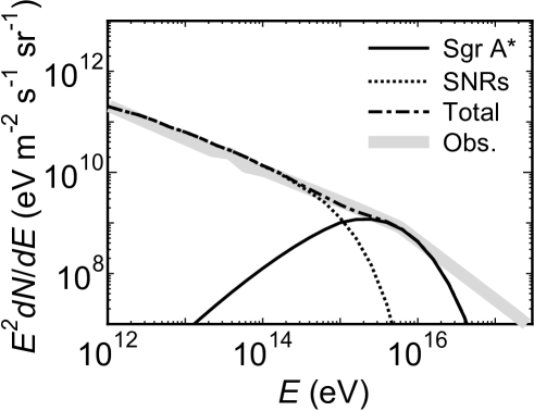
Figure 2: The spectrum of CRs injected by Sgr A* at $r=R_{\odot}$ at $t=10$ Myr (solid line). The contribution of CRs from SNRs is shown by the dotted-line and the total spectrum is shown by the dot-dashed line. The size of the halo is given by eqs. (2.11) and (3.1). Observations are shown by the gray band [64].

Figure 3: Dipole anisotropy of the arrival directions of CRs on the Earth ($r=R=R_{\odot}$, $z=0$). The dashed and the dotted lines are for the CRs injected by Sgr A* at the outburst 10 Myrs ago ($f=f_{\rm B}$; $t=10$ Myr). The dashed line is the result when $D_{\rm d}=D_{\rm h}$ and the dotted line is the one when $D_{\rm d}=0.1\>D_{\rm h}$. The solid line is for all the components ($f=f_{\rm B}+f_{\rm SNR}$) and $D_{\rm d}=0.1\>D_{\rm h}$. Recent observations with EAS-TOP [65], IceCube [66], IceTop [56], and Tibet [57] are shown by the black dots.

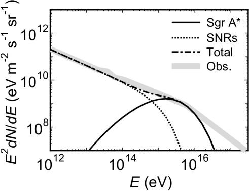
Figure 4: Same as figure 2 but for $R_{\rm h}=10$ kpc and $t=3$ Myr.

Figure 5: Same as figure 3 but for $R_{\rm h}=10$ kpc and $t=3$ Myr.

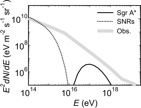
Figure 6: Same as figure 2 but for the power-law injection (eq. 4.3) at higher energies and $t=3$ Myr. The line for the total spectrum is omitted.

4 Discussion

4.1 B/C ratio

If the origin of CRs around the knee is different from that of CRs with lower energies (e.g. SNRs in the Galactic disk), the ratio of secondary to primary CR abundances can also be different. Since our model is a single-source, single-burst scenario, we can predict the ratio fairly easily. Here, we focus on the B/C ratio. Assuming that the Galactic halo is represented by an one-zone model (leaky-box-like) and that the influence of the disk can be ignored, the evolution of the total number of boron $N_{\rm B}(t)$ in the halo is written as

$$\frac{\partial N_{\rm B}}{\partial t}=-\frac{N_{\rm B}}{t_{\rm esc}}-\frac{N_{\rm B}}{\tau_{\rm B}}+\frac{N_{\rm C}}{\tau_{\rightarrow\rm B}}\>,$$ (4.1)

where $N_{\rm C}(t)$ is the carbon number, $t_{\rm esc}=R_{\rm h}^{2}/(6\rm D_{\rm h})$ is the escape time-scale of CRs from the halo, $\tau_{\rm B}$ is the spallation time-scale for boron, and $\tau_{\rightarrow\rm B}$ is the effective production time-scale for boron. We assume that primary CRs are instantaneously injected at $t=0$. Since the fraction of carbon that changes into other elements is ignorable for our fiducial model, the number of carbon evolves as $N_{\rm C}\propto\exp(-t/t_{\rm esc})$. Thus, eq. (4.1) gives the B/C ratio of

$$R_{\rm B/C}(t)\equiv\frac{N_{\rm B}(t)}{N_{\rm C}(t)}=\frac{\tau_{\rm B}}{\tau_{\rightarrow\rm B}}(1-e^{-t/\tau_{\rm B}})\>,$$ (4.2)

assuming that $N_{\rm B}=0$ at $t=0$. The leaky-box-like model represented by eq. (4.1) would be a reasonably good approximation of the diffusion model for $t\gtrsim t_{\rm esc}$, because the halo is filled with the CRs. The time-scales are related to grammages such as $\Lambda_{\rm B}=\beta c\rho\tau_{\rm B}$ and $\lambda_{\rightarrow\rm B}=\beta c\rho\tau_{\rightarrow\rm B}$, where $\beta=v/c~{}(\sim 1)$ is the particle velocity normalized by the light velocity, and $\rho$ is the typical gas density in the Galactic halo. Recent X-ray observations showed that $\rho\sim 0.002\>m_{\rm p}\>\rm cm^{-3}$ at $r\sim R_{\odot}/2=4$ kpc [67]. The escape time-scale is $t_{\rm esc}=4.6$ Myr for $R_{\rm h}=20$ kpc and $E=10^{15.5}$ eV (eq. 2.6). If we use $\Lambda_{\rm B}=9.3\>\rm g\>cm^{-2}$ and $\lambda_{\rightarrow\rm B}=26.8\>\rm g\>cm^{-2}$ [68, 69], the B/C ratio is $R_{\rm B/C}(10\rm\>Myr)\sim 0.001$, and it is independent of $E$. Observed B/C ratios can be approximated as $R_{\rm B/C,ext}\sim 0.2\>(E/{10\rm\>GeV})^{-1/3}$ for $10\lesssim E\lesssim 1000$ GeV [69, 53]. If the B/C ratio is extrapolated to $E\sim 10^{15.5}$ eV, it is $R_{\rm B/C,ext}\sim 0.003$ and is comparable to the predicted $R_{\rm B/C}$. If the observed B/C ratio is extrapolated as $R_{\rm B/C,ext}\sim 0.3\>(E/{10\rm\>GeV})^{-0.6}$ for $E\gtrsim 1$ TeV as some models suggest [69, 53], the ratio is $R_{\rm B/C,ext}\sim 10^{-4}$ at $E\sim 10^{15.5}$ eV, which is much smaller than the predicted $R_{\rm B/C}$. Anyway, a bend would be observed in the energy-B/C ratio relation as $E$ approaches the knee from smaller energies because the CRs from Sgr A* become dominant (figure 2).

4.2 Halo size

Since little is known about the size of the Galactic halo that confines the CRs around the knee, we study the CR diffusion when $R_{\rm h}$ is changed. Figure 4 is the CR spectrum at $r=R_{\odot}$ when $R_{\rm h}=R_{\rm h2}=R_{\rm h1}=10$ kpc. Since CRs escape more easily and the CR density decreases faster than when $R_{\rm h2}=20$ kpc, we chose $t=3$ Myr. The spectrum is not much different from that in figure 2. However, figure 5 shows that the anisotropy becomes larger than that in figure 3. Thus, models with a smaller $R_{\rm h}$ require a smaller $D_{\rm d}$ as well as a younger age of the FBs. Note that the flux of the CRs from SNRs is slightly smaller than that in figure 2 because those CRs also escape from the halo more easily.

4.3 Higher energy component

Recent observations have shown that CRs with higher energies ($E\sim 10^{17}$–$10^{17.5}$ eV) contain a significant fraction ($\sim 80$ %) of light elements (H and He), which suggests that they have a Galactic origin [70]. We briefly discuss whether those CRs are provided through outbursts of Sgr A*. We use eq. (2.6) as the diffusion coefficient for the halo. However, since $D_{\rm h}$ is the increasing function of CR energy, CRs with energies much larger than the knee ($E\sim 10^{17}$ eV) have already left the Galactic halo when the knee CRs arrive on the Earth ($t_{0}\sim 10$ Myr). Thus, it is difficult to attribute both the CRs around the knee and those above the knee to the same outburst about 10 Myr ago, unless an extremely large amount of CRs above the knee are generated at that outburst. Thus, we assume that the CRs with $E\sim 10^{17}$ eV were injected at another more recent outburst of Sgr A*.

Here, we do not confine acceleration mechanisms to that we explained in section 2.1.1. Thus, we adopt a generalized power-law spectrum for the CRs accelerated at Sgr A*,

$$\dot{N}(p)\propto\left(\frac{p}{p_{\rm S}}\right)^{2-\mu}\exp\left(-\frac{p_{\rm S}}{p}-\frac{p}{p_{\rm L}}\right)\>.$$ (4.3)

We assume $\mu=4$ and we set the lower and upper cutoff momenta at $p_{\rm S}c=10^{17}$ eV and at the ’ankle’ ($p_{\rm L}c=10^{18.5}$ eV), respectively. The initial distribution function for $r<r_{\rm s}$ is given by eq. (2.8), and it is zero for $r>r_{\rm s}$. We assume that $x=p/p_{\rm S}$, $t_{\rm inj}=1$ Myr, and $r_{\rm s}=0.1$ kpc. We adopt $\dot{m}=3\times 10^{-4}$ and $\eta_{\rm cr}=2\times 10^{-3}$. Figure 6 shows the CR spectrum on the Earth at $t=3$ Myr. Since $L_{\rm p,tot}t_{\rm inj}$ is 0.3% of that for figure 2 ($\dot{m}=0.1$, $\eta_{\rm cr}=2\times 10^{-3}$, and $t_{\rm inj}=1$ Myr), the scale of this outburst is relatively small. Although the injected spectrum is a power-law (eq. 4.3), the spectrum on the Earth is not. This is because part of higher-energy CRs ($E\sim 10^{18}$ eV) have already escaped from the halo. On the other hand, the observed CR spectrum between the knee and the ankle is represented by a power-law (figure 6). Thus, the CR spectrum of this energy range may be superposed by CRs produced through multiple small outbursts of Sgr A* with various $\mu$, $p_{\rm S}$, and $p_{\rm L}$. Although the predicted spectrum is smaller than the observation in figure 6, the former can be more close to the latter if we adopt a larger $\dot{m}$, $\eta_{\rm cr}$, or $t_{\rm inj}$. However, heavy elements that have a different origin may partially contribute to the observed spectrum [71, 72].

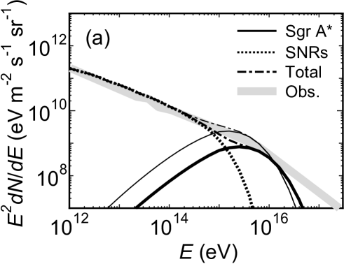
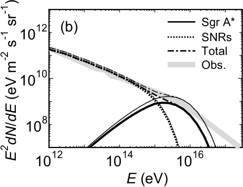
Figure 7: Same as figure 2 but parameters are slightly changed. (a) $p_{\rm eq}=1.5\>p_{\rm eq,fid}$ (thick) and $p_{\rm eq}=0.5\>p_{\rm eq,fid}$ (thin). (b) $D_{\rm h}=1.1\>D_{\rm h,fid}$ (thick) and $D_{\rm h}=0.9\>D_{\rm h,fid}$ (thin).

4.4 Allowed parameter regions

In this study, we have assumed that the CR spectrum on the Earth has three components: the SNR component ($E\lesssim 10^{14.5}$ eV), the outburst component ($10^{14.5}\lesssim E\lesssim 10^{16}$ eV), and the possible high energy component ($E\gtrsim 10^{16}$ eV). However, the observed spectrum is represented by a smooth power-law with a relatively sharp break at the knee ($E\sim 10^{15.5}$ eV) as if the spectrum were composed of only two components ($E\lesssim 10^{15.5}$ eV and $E\gtrsim 10^{15.5}$ eV). This means that the parameters related to the outburst component (the typical energy of CRs, the CR luminosity, and the diffusion coefficient in the halo) must be fine-tuned.

Figure 7a shows the CR spectrum when the typical energy of CRs is given by $p_{\rm eq}=1.5\>p_{\rm eq,fid}$ or $0.5\>p_{\rm eq,fid}$, where $p_{\rm eq,fid}$ is the fiducial value adopted in figure 2 (eq. 2.1). Other parameters are the same as those for figure 2. If we change $p_{\rm eq}$ further while fixing the SNR component, the sharp break at the knee is impaired. Thus, the spectrum would look like being composed of three components if we include a fixed high energy component ($E\gtrsim 10^{16}$ eV). The same happens when the coefficient of the CR luminosity is changed to be $\eta_{\rm cr}\gtrsim 1.5\>\eta_{\rm cr,fid}$ or $\eta_{\rm cr}\lesssim(2/3)\>\eta_{\rm cr,fid}$, where $\eta_{\rm cr,fid}=2\times 10^{-3}$ is the fiducial value adopted in figure 2. Figure 7b shows the CR spectrum when the diffusion coefficient in the halo is given by $D_{\rm h}=1.1\>D_{\rm h,fid}$ or $0.9\>D_{\rm h,fid}$, where $D_{\rm h,fid}$ is the fiducial value adopted in figure 2 (eq. 2.6). If we further change the diffusion coefficient, the spectrum shifts notably. In this case, however, the overall shape of the spectrum does not much change and the sharp break at the knee is conserved.

4.5 Gamma-rays from other galaxies

We have shown that a past explosive activity of Sgr A* can provide CRs around the knee observed on the Earth. Since those CRs have been distributed widely in the Galaxy and they are not strongly concentrated around Sgr A* (figure 1), it would be difficult to confirm our model based on their distribution. However, similar AGN activities may be happening in other galaxies. If we observe those galaxies during or just after the outburst of the nucleus, ejected PeV CRs may be concentrated around their center. Moreover, if those galaxies have enough amount of molecular gas around their center and if it serves as the target of $pp$-interaction, gamma-rays of sub-PeV could be produced. Although most of them are absorbed by the extragalactic background light, photons of a few tens of TeV produced by electromagnetic cascades could be observable in the future as follows.

The total energy of protons injected by an AGN is written as

$$L_{\rm p,tot}t_{\rm inj} = \eta_{\rm cr}\dot{m}L_{\rm Edd}t_{\rm inj}$$ (4.4)

$$= 3.5\times 10^{54}\left(\frac{\eta_{\rm cr}}{2\times 10^{-3}}\right)\left(\frac{\dot{m}}{0.1}\right)\left(\frac{L_{\rm Edd}}{5.5\times 10^{44}\rm\>erg\>s^{-1}}\right)\left(\frac{t_{\rm inj}}{\rm Myr}\right)\rm\>erg\>.$$

We normalized the Eddington luminosity by that for Sgr A*. The time scale of $pp$-interaction is given by

$$t_{pp} \sim 1/(\sigma_{pp}n_{\rm MC}c)$$ (4.5)

$$= 1.6\times 10^{5}\left(\frac{n_{\rm MC}}{100\rm\>cm^{-3}}\right)^{-1}\rm\>yr\>,$$

where $\sigma_{pp}$ is the inelastic cross section for the $pp$-interaction, and $n_{\rm MC}$ is the number density of target protons in the molecular gas. We assumed that $\sigma_{pp}=6.6\times 10^{-26}\rm\>cm^{2}$ for CR protons with $E\sim 10^{15.5}$ eV [73]. Assuming that the protons are still confined around the galactic center, the gamma-ray luminosity of molecular gas around the center is given by

$$L_{\gamma} \sim f_{\rm MCe}L_{\rm p,tot}t_{\rm inj}/t_{pp}$$ (4.6)

$$= 6.8\times 10^{39}\left(\frac{f_{\rm MCe}}{0.01}\right)\left(\frac{L_{\rm p,tot}t_{\rm inj}}{3.5\times 10^{54}\rm\>erg}\right)\left(\frac{t_{pp}}{1.6\times 10^{5}\rm\>yr}\right)^{-1}\rm\>erg\>s^{-1}\>,$$

where $f_{\rm MCe}=f_{\rm MC}\min\{t_{\rm diff}/t_{pp},1\}$ is the effective filling factor and $f_{\rm MC}$ is the filling factor of the molecular gas. If the diffusion time-scale $t_{\rm diff}$ is smaller than $t_{pp}$, a significant fraction of CR protons escape from the molecular gas before they interact with protons in the gas. We normalized $L_{\rm p,tot}t_{\rm inj}$ by our fiducial value. If the distance to this galaxy is $d=30$ Mpc, the gamma-ray flux is $f_{\gamma}=L_{\gamma}/(4\pi d^{2})\sim 6.3\times 10^{-14}\rm\>erg\>cm^{-2}\>s^{-1}$, which could be observed with LHASSO [74]. If the flux is larger (e.g. larger $f_{\rm MC}$ or smaller $d$), the galaxy could be detected with the Cherenkov Telescope Array (CTA) [75]. Neutrinos are additionally generated through $pp$-interaction. However, since the expected flux is comparable to the gamma-ray flux, it would be difficult to detect them in the near future.

Gamma-rays are also created inside the RIAF, but high-energy gamma-rays are absorbed by thermal photons there. Only photons of $E\lesssim 1$ GeV can escape from the RIAF [20]. The gamma-ray luminosity is $\sim 0.1L_{\rm p,tot}$ [20], which means the flux of $\sim 2\times 10^{-13}\rm\>erg\>s^{-1}\>cm^{-2}$ for $d=30$ Mpc. This is marginally detectable by Fermi, although gamma-rays from LLAGNs are hardly detected so far [76]. Neutrinos are also produced inside the RIAF, and the neutrino flux is almost the same as the gamma-ray flux, which is too low to be detected in the near future.

5 Recent CR injection from Sgr A*, and the gamma-rays and neutrinos from the CMZ

In Paper I, we indicated that the TeV gamma-rays observed at the CMZ are generated by CRs recently ($\sim 10^{5}$ yr) injected by Sgr A*. Since the gamma-ray data have been updated with HESS [77], we revisit our model here to show the consistency of our model with the latest data.

We assume that the activities of Sgr A* in the normal state, in which Sgr A* stays most of the time, are much weaker than those in the outburst state, although they are much stronger than the activities in the current faint state over the past $\sim 50$ yrs [25, 26, 27, 28]. The CR acceleration in the normal state may be much different from that in the outburst state. The CRs responsible for the observed gamma-rays from the CMZ may be accelerated during the normal state. Motivated by the HESS observations that have shown that the CR spectrum in the CMZ is described by a power-law [77], we assume that the spectrum of the CRs accelerated at Sgr A* in the normal state is given by eq. (4.3). The power-law spectrum may be realized when the disk of the RIAF has a power-law structure and $E_{\rm p,eq}$ in eq. (2.1) changes with the radius. Alternatively, CR acceleration may occur at a vacuum gap in the black hole magnetosphere [19, 24]. Here, we chose $\mu=4.07$, $p_{\rm S}c=9\times 10^{11}$ eV, and $p_{\rm L}c=1\times 10^{16}$ eV to be consistent with the gamma-ray observations. The CRs are injected at the Galactic center ($r=0$). The normalization of eq. (4.3) is given so that the energy injection rate is $\lambda\eta_{\rm cr}\dot{M}c^{2}$, where $\lambda$ is the fraction of CRs that enter the CMZ. For the convenience to calculate gamma-ray emission, we treat the diffusion of those CRs only in the direction of the disk-like CMZ and we solve a spherically symmetric diffusion equation,

$$\frac{\partial f_{\rm R}}{\partial t}=\frac{1}{r^{2}}\frac{\partial}{\partial r}\left(r^{2}D_{\rm d}(p)\frac{\partial f_{\rm R}}{\partial r}\right)+Q\>,$$ (5.1)

where $f_{\rm R}=f_{\rm R}(t,r,p)$ is the distribution function for the recently injected CRs. The source term in Eq. (5.1) is written as $\int 4\pi cp^{3}Qdp=\lambda\eta_{\rm cr}\dot{M}c^{2}$. Since the size of the CMZ ($\sim 100$ pc) is much larger than that of the RIAF, we treat $Q$ as a point source. We consider this component $f_{\rm R}$ only for $r\lesssim H_{\rm d}$ because those CRs contribute little to the CRs in the halo at present (see figure 1). We assume that the injection of those CRs is steady and the left-hand side of eq.(5.1) is zero. The diffusion coefficient in the CMZ is the same as that for the Galactic disk $D_{\rm d}$ (eq. 3.3). In the following calculations, we take $\eta_{\rm cr}=2\times 10^{-3}$, which is the same as that for the outburst component (section 2.1.1), and $\dot{m}=0.001$, which is the same as that adopted in Paper I. We also assume that $\lambda=0.015$ to be consistent with observations. Since the diffusion time of CRs in the CMZ is $\sim 10^{4}$ yr at $E\sim 10$ TeV, the results do not much change even if $\dot{m}=0$ after the outburst $\sim 10^{7}$ years ago and before $\sim 10^{4}$ years ago. On the other hand, we assume that the activities of Sgr A* during this period is not too large to affect the CRs observed on the Earth at present. The most recent inactivity of Sgr A* in the past $\sim 50$ years does not affect the results and can be ignored.

Neutrinos and gamma-rays are produced via the interactions between the CRs and target nucleons in the CMZ. The size of the CMZ is given by $R_{\rm c}$ and the molecular gas is uniformly distributed for $r<R_{\rm c}$. From Paper I, we assume that $R_{\rm c}=130$ pc, and the gas density of the CMZ is $\rho_{\rm c}=1.4\times 10^{-22}\rm\>g\>cm^{-3}$. We calculate the production rate of gamma-ray photons and neutrinos by pion decay using the formula provided by Ref. [73].

Using the results shown in figure 3 of Ref. [78], we estimate the attenuation of very high energy gamma-rays by pair production on the Galactic interstellar radiation field. However, the attenuation does not much affect the following results. The energy density of interstellar radiation field ($\sim 10\rm\;eV\>cm^{-3}$) is much smaller than probable magnetic fields in the CMZ, the gamma-ray emission via inverse Compton scattering by secondary electrons can be ignored [12].

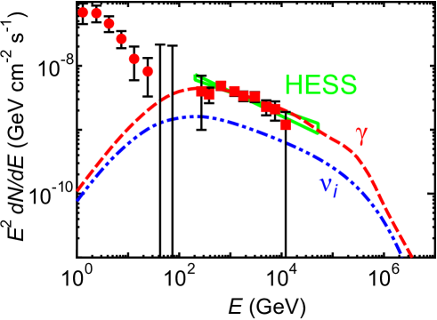
Figure 8: Predicated $\gamma$-ray flux (dashed line) and neutrino flux per flavor (two-dot dashed line) from the CMZ. Filled circles and squares are the Fermi and HESS observations, respectively [79, 29]. Recent HESS observations (Ref. [77]) are shown by the ribbon assuming that the luminosity of the observed region is a factor of two smaller than that of Ref [29].

Figure 1 shows the radial distribution of this CR component, which indicates that their influence is confined to the vicinity of the Galactic center. Figure 8 shows the gamma-ray and neutrino spectra of the CMZ. For $E\gtrsim 0.4$ TeV, the $\gamma$-ray spectrum is consistent with the HESS observations. The spectrum extends even to $E\gtrsim 10$ TeV, which is consistent with the recent report for the inner region of the CMZ [77]. In our model, associated 10-100 TeV neutrinos (figure 8) may be detectable with KM3Net [80]. The expected sensitivity is $\sim{\rm a~{}few}\times{10}^{-9}~{}{\rm GeV}~{}{\rm cm}^{-2}~{}{\rm s}^{-1}$, so the detection would be feasible with many years of observations. The $\gamma$-rays from the CMZ at $E\sim 100$ TeV (figure 8) may be detected with CTA [75]. Note that the point-like gamma-ray source HESS J1745–290 may be the direct emission from Sgr A* and may reflect its current activity.

6 Power-law CR spectrum at the outburst of Sgr A*

In the fiducial model in section 3, we take a typical spectrum of stochastic acceleration for the CR spectrum at the outburst of Sgr A* (eq. 2.2). Here, we consider a power-law spectrum for the outburst, because the CR spectrum for the recent injection is a power-law (section 5).

We calculate the CR spectrum on the Earth when the CR spectrum at the outburst is given by eq. (2.8) in which $\dot{N}$ is replaced by the power-law form (eq. 4.3). The total energy injection rate of the CRs is given by $L_{\rm p,tot}t_{\rm inj}$ (section 2.1.3) and the value is the same as that for the fiducial model ($\dot{m}=0.1$, $\eta_{\rm cr}=2\times 10^{-3}$, and $t_{\rm inj}=1$ Myr). The cutoff momentums ($p_{\rm S}c=9\times 10^{11}$ eV, and $p_{\rm L}c=1\times 10^{16}$ eV) are the same as those for the recently injected component that can explain the gamma-ray data observed with HESS (section 5). The lower-cutoff may be determined by the advection of CRs by some outflows. Moreover, we set $x=p/p_{\rm S}$ in eq. (2.8). As is the case of the fiducial model, we assume that $r_{\rm s}=0.1$ kpc, and the initial distribution function for $r>r_{\rm s}$ is zero.

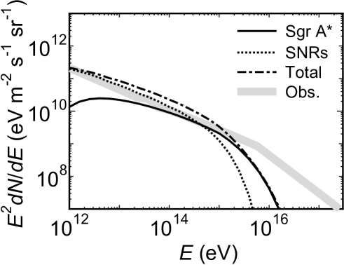
Figure 9: Same as figure 2 but for the power-law injection (eq. 4.3) similar to the recent injection (figure 8).

In figure 9, we show the CR spectra on the Earth at $t=10$ Myr. It shows that the CR flux is almost comparable to that from the SNRs and suggests that Sgr A* alone could provide enough CRs that are detected on the Earth. However, the slope of the spectrum does not match the observation and the spectrum is curved. This is because the CR injection from Sgr A* is instantaneous; higher-energy CRs have already arrived on the Earth while most of lower-energy CRs have not, which is the same reason for the curve of the anisotropy plot (figure 3). Moreover, the highest-energy CRs ($E\gtrsim 10^{15}$ eV) have started to escape from the Galactic halo, which decreases the number density of those CRs on the Earth. These facts suggest that it would be difficult to explain the CR spectrum on the Earth only by those accelerated by Sgr A* with the same spectral form observed at the CMZ. To be consistent with both the latest HESS data for the CMZ and the CR flux on the Earth, the acceleration mechanism at the outburst of Sgr A* may need to be somewhat different from that for the recent injection.

7 Conclusions

We have shown that a past intense activity of Sgr A*, which created the Fermi bubbles $\sim 10$ Myr ago, can significantly contribute as a “Pevatron” to the Galactic CRs around the knee ($E\sim 10^{15.5}$ eV) observed on the Earth. The diffusion coefficient in the halo is estimated on the condition that the CRs are prevailing in the halo at present. We solved a diffusion equation for the CRs and reproduced the observed CR flux around the knee. The observed small anisotropy of the arrival directions of the CRs is compatible with the prediction if the diffusion coefficient in the Galactic disk is smaller than that in the halo, which is reasonable. Our model predicts that the boron-to-carbon ratio is independent of CR energy at energies close to the knee if the CRs from Sgr A* are dominant around that energy. Gamma-ray emissions could be observed in nearby galaxies, if similar activities are happening there. It is unlikely that the spectrum of the CRs accelerated at the outburst of Sgr A* is described by a power-law with a large energy range in contrast with the CR spectrum suggested from the gamma-ray observations of the CMZ. This may mean that the CR acceleration mechanism at the outburst could be different from that in the normal state of Sgr A*.

Although our single-source scenario may be rather extreme and some tuning is necessary to fit the observed CR flux smoothly, surprisingly such models are not ruled out by the present data. Thus, our results imply that Sgr A* should be examined as one of the potential sources of CRs around the knee, whose origin has been discussed for many years (e.g., [81, 82]). We still cannot deny the possibility that SNRs are still the main sources for the CRs around the knee, and proposed ideas including faster acceleration at oblique shocks [83, 84], contributions from Type IIn and Type IIb supernovae [85, 86, 87], and early acceleration at dense stellar winds [88, 86, 89]. A different source population such as super-bubbles has also been considered (e.g., [90, 91]). However, our study motivates investigations into the roles of the Galactic center in CR production, possibilities of a single source origin, and so on [92]. We note that models with a recent local source may give results similar to ours. If the source exploded near the Earth and the PeV CRs have already diffused out on a scale much larger than the distance to the source, the anisotropy of the arrival directions can be small. However, a problem of these models is that the same sources are likely to be widely distributed in the Galaxy especially if the PeV CR source is an SNR. This encounters the difficulty mentioned in section 1 that there is little observational evidence implicating SNRs as Pevatrons.

Appendix A Analytical solutions for the diffusion equation

If the Galactic disk can be ignored, the diffusion of CRs in the spherical halo can be analytically solved. The diffusion equation is

$$\frac{\partial f}{\partial t}=\frac{1}{r^{2}}\frac{\partial}{\partial r}\left(r^{2}D_{\rm h}(p)\frac{\partial f}{\partial r}\right)\>,$$ (A.1)

where $f=f(t,r,p)$ is the distribution function. We assume that $f=0$ at $r=R_{\rm h}$ and $\partial f/\partial r=0$ at $r=0$. In eq. (A.1), $D_{\rm h}$ can be treated as a constant for a given $p$. Using the separation of variable method, eq. (2.7) is represented as

$$\frac{1}{r^{2}R}\frac{d}{dr}\left(r^{2}\frac{dR}{dr}\right)=\frac{1}{D_{\rm h}T}\frac{\partial T}{\partial t}$$ (A.2)

for $f(t,r,p)=R(r)T(t,p)$. This equation makes sense when both sides are equal to a negative constant $-\xi^{2}$. Thus, we obtain two equations:

$$\frac{\partial T}{\partial t}+\xi^{2}D_{\rm h}T=0\>,$$ (A.3)

$$\frac{1}{r^{2}}\frac{d}{dr}\left(r^{2}\frac{dR}{dr}\right)+\xi^{2}R=0.$$ (A.4)

The solution for eq. (A.3) is

$$T(t,p)=A\exp(-D_{\rm h}(p)\xi^{2}t)\>,$$ (A.5)

where $A$ is the constant. The solution of eq. (A.4) is

$$R(r)=B^{\prime}\frac{\sin(\xi r)}{r}+C^{\prime}\frac{\cos(\xi r)}{r}=B^{\prime}\frac{\sin(\xi r)}{r}\>,$$ (A.6)

where $B^{\prime}$ and $C^{\prime}$ are the constants, and $C^{\prime}$ must be zero because $f$ is finite at $r=0$. Because of the boundary condition at $r=R_{\rm h}$, the eigenvalue satisfies

$$\xi_{n}=n\pi/R_{\rm h}$$ (A.7)

and the eigenfunctions are

$$R_{n}(r)=B^{\prime}_{n}\frac{\sin(\xi_{n}r)}{r}$$ (A.8)

for $n=1,2,3,...$.

Thus, the solution for the number $n$ is

$$f_{n}(t,r,p)=R_{n}(r)T(t,p)=\frac{A_{n}}{r}\sin(\xi_{n}r)\exp(-D_{\rm h}(p)\xi_{n}^{2}t)\>,$$ (A.9)

where $A_{n}=AB^{\prime}_{n}$. The general solution is given by their superposition:

$$f(t,r,p)=\sum_{n=1}^{\infty}f_{n}(t,r,p)=\sum_{n=1}^{\infty}\frac{A_{n}}{r}\sin(\xi_{n}r)\exp(-D_{\rm h}(p)\xi_{n}^{2}t)\>.$$ (A.10)

The coefficients $A_{n}$ can be determined by the initial condition at $t=0$:

$$f(0,r,p)=\sum_{n=1}^{\infty}\frac{A_{n}}{r}\sin(\xi_{n}r)\>.$$ (A.11)

Since this is a Fourier series, the coefficients are given by

$$A_{n}(p)=\frac{2}{R_{\rm h}}\int_{0}^{R_{\rm h}}f(0,r^{\prime},p)\sin(\xi_{n}r^{\prime})r^{\prime}dr^{\prime}\>.$$ (A.12)

References

- [1] K. Koyama, R. Petre, E. V. Gotthelf, U. Hwang, M. Matsuura, M. Ozaki et al., Evidence for shock acceleration of high-energy electrons in the supernova remnant SN1006, Nature 378 (Nov., 1995) 255–258.
- [2] M. Tavani, A. Giuliani, A. W. Chen, A. Argan, G. Barbiellini, A. Bulgarelli et al., Direct Evidence for Hadronic Cosmic-Ray Acceleration in the Supernova Remnant IC 443, Astrophys. J. 710 (Feb., 2010) L151–L155, [1001.5150].
- [3] M. Ackermann, M. Ajello, A. Allafort, L. Baldini, J. Ballet, G. Barbiellini et al., Detection of the Characteristic Pion-Decay Signature in Supernova Remnants, Science 339 (Feb., 2013) 807–811, [1302.3307].
- [4] A. R. Bell, Cosmic ray acceleration, Astroparticle Physics 43 (Mar., 2013) 56–70.
- [5] D. Caprioli and A. Spitkovsky, Simulations of Ion Acceleration at Non-relativistic Shocks. II. Magnetic Field Amplification, Astrophys. J. 794 (Oct., 2014) 46, [1401.7679].
- [6] D. Caprioli and A. Spitkovsky, Simulations of Ion Acceleration at Non-relativistic Shocks. III. Particle Diffusion, Astrophys. J. 794 (Oct., 2014) 47, [1407.2261].
- [7] T. N. Kato, Particle Acceleration and Wave Excitation in Quasi-parallel High-Mach-number Collisionless Shocks: Particle-in-cell Simulation, Astrophys. J. 802 (Apr., 2015) 115, [1407.1971].
- [8] R. Schlickeiser, Cosmic Ray Astrophysics. 2002.
- [9] D. Caprioli, Cosmic-ray Acceleration and Propagation, ArXiv e-prints (Oct., 2015) , [1510.07042].
- [10] V. A. Acciari, E. Aliu, T. Arlen, T. Aune, M. Beilicke, W. Benbow et al., Discovery of TeV Gamma-ray Emission from Tycho’s Supernova Remnant, Astrophys. J. 730 (Apr., 2011) L20, [1102.3871].
- [11] F. A. Aharonian, Gamma rays from supernova remnants, Astroparticle Physics 43 (Mar., 2013) 71–80.
- [12] Y. Fujita, S. S. Kimura and K. Murase, Hadronic origin of multi-TeV gamma rays and neutrinos from low-luminosity active galactic nuclei: Implications of past activities of the Galactic center, Phys. Rev. D 92 (July, 2015) 023001, [1506.05461].
- [13] F. Aharonian and A. Neronov, TeV Gamma Rays From the Galactic Center Direct and Indirect Links to the Massive Black Hole in Sgr A, Astrophysics and Space Science 300 (Nov., 2005) 255–265.
- [14] D. R. Ballantyne, F. Melia, S. Liu and R. M. Crocker, A Possible Link between the Galactic Center HESS Source and Sagittarius A*, Astrophys. J. 657 (Mar., 2007) L13–L16, [astro-ph/0701709].
- [15] M. Chernyakova, D. Malyshev, F. A. Aharonian, R. M. Crocker and D. I. Jones, The High-energy, Arcminute-scale Galactic Center Gamma-ray Source, Astrophys. J. 726 (Jan., 2011) 60, [1009.2630].
- [16] Y.-Q. Guo, Z. Tian, Z. Wang, H.-J. Li and T.-L. Chen, The Galactic Center: A PeV Cosmic Ray Acceleration Factory, ArXiv e-prints (Apr., 2016) , [1604.08301].
- [17] S. Celli, A. Palladino and F. Vissani, Multi-TeV gamma-rays and neutrinos from the Galactic Center region, ArXiv e-prints (Apr., 2016) , [1604.08791].
- [18] R.-Y. Liu, X.-Y. Wang, A. Prosekin and X.-C. Chang, Modeling the gamma-ray emission in the Galactic Center with a fading cosmic-ray accelerator, ArXiv e-prints (Sept., 2016) , [1609.01069].
- [19] H. Krawczynski, X-Ray and TeV Gamma-Ray Emission from Parallel Electron-Positron or Electron-Proton Beams in BL Lacertae Objects, Astrophys. J. 659 (Apr., 2007) 1063–1073, [astro-ph/0610641].
- [20] S. S. Kimura, K. Murase and K. Toma, Neutrino and Cosmic-Ray Emission and Cumulative Background from Radiatively Inefficient Accretion Flows in Low-luminosity Active Galactic Nuclei, Astrophys. J. 806 (June, 2015) 159, [1411.3588].
- [21] M. Hoshino, Angular Momentum Transport and Particle Acceleration During Magnetorotational Instability in a Kinetic Accretion Disk, Physical Review Letters 114 (Feb., 2015) 061101, [1502.02452].
- [22] K. Murase, D. Guetta and M. Ahlers, Hidden Cosmic-Ray Accelerators as an Origin of TeV-PeV Cosmic Neutrinos, Physical Review Letters 116 (Feb., 2016) 071101, [1509.00805].
- [23] S. S. Kimura, K. Toma, T. K. Suzuki and S.-i. Inutsuka, Stochastic Particle Acceleration in Turbulence Generated by Magnetorotational Instability, Astrophys. J. 822 (May, 2016) 88, [1602.07773].
- [24] K. Ptitsyna and A. Neronov, Particle acceleration in the vacuum gaps in black hole magnetospheres, Astron. Astrophys. 593 (Aug., 2016) A8, [1510.04023].
- [25] K. Koyama, Y. Maeda, T. Sonobe, T. Takeshima, Y. Tanaka and S. Yamauchi, ASCA View of Our Galactic Center: Remains of Past Activities in X-Rays?, Publ. Astron. Soc. Jpn. 48 (Apr., 1996) 249–255.
- [26] H. Murakami, K. Koyama, M. Sakano, M. Tsujimoto and Y. Maeda, ASCA Observations of the Sagittarius B2 Cloud: An X-Ray Reflection Nebula, Astrophys. J. 534 (May, 2000) 283–290.
- [27] T. Totani, A RIAF Interpretation for the Past Higher Activity of the Galactic Center Black Hole and the 511 keV Annihilation Emission, Publ. Astron. Soc. Jpn. 58 (Dec., 2006) 965–977.
- [28] S. G. Ryu, M. Nobukawa, S. Nakashima, T. G. Tsuru, K. Koyama and H. Uchiyama, X-Ray Echo from the Sagittarius C Complex and 500-year Activity History of Sagittarius A*, Publ. Astron. Soc. Jpn. 65 (Apr., 2013) 33.
- [29] F. Aharonian, A. G. Akhperjanian, A. R. Bazer-Bachi, M. Beilicke, W. Benbow, D. Berge et al., Discovery of very-high-energy -rays from the Galactic Centre ridge, Nature 439 (Feb., 2006) 695–698, [astro-ph/0603021].
- [30] I. Cholis, C. Evoli, F. Calore, T. Linden, C. Weniger and D. Hooper, The Galactic Center GeV excess from a series of leptonic cosmic-ray outbursts, J. Cosmol. Astropart. Phys. 12 (Dec., 2015) 005, [1506.05119].
- [31] M. G. Aartsen, R. Abbasi, Y. Abdou, M. Ackermann, J. Adams, J. A. Aguilar et al., First Observation of PeV-Energy Neutrinos with IceCube, Physical Review Letters 111 (July, 2013) 021103, [1304.5356].
- [32] IceCube Collaboration, Evidence for High-Energy Extraterrestrial Neutrinos at the IceCube Detector, Science 342 (Nov., 2013) 1242856, [1311.5238].
- [33] M. G. Aartsen, M. Ackermann, J. Adams, J. A. Aguilar, M. Ahlers, M. Ahrens et al., Observation of High-Energy Astrophysical Neutrinos in Three Years of IceCube Data, Physical Review Letters 113 (Sept., 2014) 101101, [1405.5303].
- [34] M. G. Aartsen, M. Ackermann, J. Adams, J. A. Aguilar, M. Ahlers, M. Ahrens et al., Atmospheric and astrophysical neutrinos above 1 TeV interacting in IceCube, Phys. Rev. D 91 (Jan., 2015) 022001, [1410.1749].
- [35] C. K. Cramphorn and R. A. Sunyaev, Interstellar gas in the Galaxy and the X-ray luminosity of Sgr A∗ in the recent past, Astron. Astrophys. 389 (July, 2002) 252–270.
- [36] G. Ponti, M. R. Morris, M. Clavel, R. Terrier, A. Goldwurm, S. Soldi et al., On the past activity of Sgr A*, in IAU Symposium (L. O. Sjouwerman, C. C. Lang and J. Ott, eds.), vol. 303 of IAU Symposium, pp. 333–343, May, 2014. DOI.
- [37] M. Su, T. R. Slatyer and D. P. Finkbeiner, Giant Gamma-ray Bubbles from Fermi-LAT: Active Galactic Nucleus Activity or Bipolar Galactic Wind?, Astrophys. J. 724 (Dec., 2010) 1044–1082, [1005.5480].
- [38] R. M. Crocker and F. Aharonian, Fermi Bubbles: Giant, Multibillion-Year-Old Reservoirs of Galactic Center Cosmic Rays, Physical Review Letters 106 (Mar., 2011) 101102, [1008.2658].
- [39] R. M. Crocker, Non-thermal insights on mass and energy flows through the Galactic Centre and into the Fermi bubbles, Mon. Not. R. Astron. Soc. 423 (July, 2012) 3512–3539, [1112.6247].
- [40] K. Sasaki, K. Asano and T. Terasawa, Time-dependent Stochastic Acceleration Model for Fermi Bubbles, Astrophys. J. 814 (Dec., 2015) 93, [1510.02869].
- [41] K. Zubovas, A. R. King and S. Nayakshin, The Milky Way’s Fermi bubbles: echoes of the last quasar outburst?, Mon. Not. R. Astron. Soc. 415 (July, 2011) L21–L25, [1104.5443].
- [42] F. Guo and W. G. Mathews, The Fermi Bubbles. I. Possible Evidence for Recent AGN Jet Activity in the Galaxy, Astrophys. J. 756 (Sept., 2012) 181, [1103.0055].
- [43] H.-Y. K. Yang, M. Ruszkowski, P. M. Ricker, E. Zweibel and D. Lee, The Fermi Bubbles: Supersonic Active Galactic Nucleus Jets with Anisotropic Cosmic-Ray Diffusion, Astrophys. J. 761 (Dec., 2012) 185, [1207.4185].
- [44] K. Zubovas and S. Nayakshin, Fermi bubbles in the Milky Way: the closest AGN feedback laboratory courtesy of Sgr A*?, Mon. Not. R. Astron. Soc. 424 (July, 2012) 666–683, [1203.3060].
- [45] Y. Fujita, Y. Ohira and R. Yamazaki, The Fermi Bubbles as a Scaled-up Version of Supernova Remnants, Astrophys. J. 775 (Sept., 2013) L20, [1308.5228].
- [46] Y. Fujita, Y. Ohira and R. Yamazaki, A Hadronic-leptonic Model for the Fermi Bubbles: Cosmic-Rays in the Galactic Halo and Radio Emission, Astrophys. J. 789 (July, 2014) 67, [1405.5214].
- [47] A. M. Taylor and G. Giacinti, Cosmic Rays in a Galactic Breeze, ArXiv e-prints (July, 2016) , [1607.08862].
- [48] M. Giler, Cosmic rays from the galactic centre, Journal of Physics G Nuclear Physics 9 (Sept., 1983) 1139–1149.
- [49] F. Yuan and R. Narayan, Hot Accretion Flows Around Black Holes, Ann. Rev. Astron. Astrophys. 52 (Aug., 2014) 529–588, [1401.0586].
- [50] S. Gillessen, F. Eisenhauer, S. Trippe, T. Alexander, R. Genzel, F. Martins et al., Monitoring Stellar Orbits Around the Massive Black Hole in the Galactic Center, Astrophys. J. 692 (Feb., 2009) 1075–1109, [0810.4674].
- [51] P. A. Becker, T. Le and C. D. Dermer, Time-dependent Stochastic Particle Acceleration in Astrophysical Plasmas: Exact Solutions Including Momentum-dependent Escape, Astrophys. J. 647 (Aug., 2006) 539–551, [astro-ph/0604504].
- [52] N. Tomassetti, Origin of the Cosmic-Ray Spectral Hardening, Astrophys. J. 752 (June, 2012) L13, [1204.4492].
- [53] D. Benyamin, E. Nakar, T. Piran and N. J. Shaviv, Recovering the Observed B/C Ratio in a Dynamic Spiral-armed Cosmic Ray Model, Astrophys. J. 782 (Feb., 2014) 34, [1308.1727].
- [54] R. Jansson and G. R. Farrar, A New Model of the Galactic Magnetic Field, Astrophys. J. 757 (Sept., 2012) 14, [1204.3662].
- [55] M. C. Beck, A. M. Beck, R. Beck, K. Dolag, A. W. Strong and P. Nielaba, New constraints on modelling the random magnetic field of the MW, J. Cosmol. Astropart. Phys. 5 (May, 2016) 056, [1409.5120].
- [56] M. G. Aartsen, R. Abbasi, Y. Abdou, M. Ackermann, J. Adams, J. A. Aguilar et al., Observation of Cosmic-Ray Anisotropy with the IceTop Air Shower Array, Astrophys. J. 765 (Mar., 2013) 55, [1210.5278].
- [57] M. Amenomori, X. J. Bi, D. Chen, T. L. Chen, W. Y. Chen, S. W. Cui et al., Northern Sky Galactic Cosmic Ray Anisotropy between 10 and 1000 TeV with the Tibet Air Shower Array, Astrophys. J. 836 (Feb., 2017) 153, [1701.07144].
- [58] J. Skilling, Cosmic ray streaming. III - Self-consistent solutions, Mon. Not. R. Astron. Soc. 173 (Nov., 1975) 255–269.
- [59] B. A. Keeney, C. W. Danforth, J. T. Stocke, S. V. Penton, J. M. Shull and K. R. Sembach, Does the Milky Way Produce a Nuclear Galactic Wind?, Astrophys. J. 646 (Aug., 2006) 951–964, [astro-ph/0604323].
- [60] N. Senno, P. Mészáros, K. Murase, P. Baerwald and M. J. Rees, Extragalactic Star-forming Galaxies with Hypernovae and Supernovae as High-energy Neutrino and Gamma-ray Sources: the case of the 10 TeV Neutrino data, Astrophys. J. 806 (June, 2015) 24, [1501.04934].
- [61] G. Case and D. Bhattacharya, Revisiting the galactic supernova remnant distribution., Astron. Astrophys. Sup. 120 (Dec., 1996) 437–440.
- [62] P. Blasi and E. Amato, Diffusive propagation of cosmic rays from supernova remnants in the Galaxy. I: spectrum and chemical composition, J. Cosmol. Astropart. Phys. 1 (Jan., 2012) 010.
- [63] Y. Fujita, F. Takahara, Y. Ohira and K. Iwasaki, Alfvén wave amplification and self-containment of cosmic rays escaping from a supernova remnant, Mon. Not. R. Astron. Soc. 415 (Aug., 2011) 3434–3438, [1105.0683].
- [64] K. Kotera and A. V. Olinto, The Astrophysics of Ultrahigh-Energy Cosmic Rays, Ann. Rev. Astron. Astrophys. 49 (Sept., 2011) 119–153, [1101.4256].
- [65] M. Aglietta, V. V. Alekseenko, B. Alessandro, P. Antonioli, F. Arneodo, L. Bergamasco et al., Evolution of the Cosmic-Ray Anisotropy Above 1014 eV, Astrophys. J. 692 (Feb., 2009) L130–L133, [0901.2740].
- [66] R. Abbasi, Y. Abdou, T. Abu-Zayyad, M. Ackermann, J. Adams, J. A. Aguilar et al., Observation of Anisotropy in the Galactic Cosmic-Ray Arrival Directions at 400 TeV with IceCube, Astrophys. J. 746 (Feb., 2012) 33, [1109.1017].
- [67] J. Kataoka, M. Tahara, T. Totani, Y. Sofue, Y. Inoue, S. Nakashima et al., Global Structure of Isothermal Diffuse X-Ray Emission along the Fermi Bubbles, Astrophys. J. 807 (July, 2015) 77, [1505.05936].
- [68] W. R. Webber, J. C. Kish and D. A. Schrier, Individual charge changing fragmentation cross sections of relativistic nuclei in hydrogen, helium, and carbon targets, Phys. Rev. C 41 (Feb., 1990) 533–546.
- [69] A. Obermeier, P. Boyle, J. Hörandel and D. Müller, The Boron-to-carbon Abundance Ratio and Galactic Propagation of Cosmic Radiation, Astrophys. J. 752 (June, 2012) 69, [1204.6188].
- [70] S. Buitink, A. Corstanje, H. Falcke, J. R. Hörandel, T. Huege, A. Nelles et al., A large light-mass component of cosmic rays at 1017-1017.5 electronvolts from radio observations, Nature 531 (Mar., 2016) 70–73, [1603.01594].
- [71] W. D. Apel, J. C. Arteaga-Velàzquez, K. Bekk, M. Bertaina, J. Blümer, H. Bozdog et al., Ankle-like feature in the energy spectrum of light elements of cosmic rays observed with KASCADE-Grande, Phys. Rev. D 87 (Apr., 2013) 081101, [1304.7114].
- [72] S. Thoudam, J. P. Rachen, A. van Vliet, A. Achterberg, S. Buitink, H. Falcke et al., Cosmic-ray energy spectrum and composition up to the ankle: the case for a second Galactic component, Astron. Astrophys. 595 (Oct., 2016) A33, [1605.03111].
- [73] S. R. Kelner, F. A. Aharonian and V. V. Bugayov, Energy spectra of gamma rays, electrons, and neutrinos produced at proton-proton interactions in the very high energy regime, Phys. Rev. D 74 (Aug., 2006) 034018, [astro-ph/0606058].
- [74] J. Knödlseder, The future of gamma-ray astronomy, Comptes Rendus Physique 17 (June, 2016) 663–678, [1602.02728].
- [75] M. Actis, G. Agnetta, F. Aharonian, A. Akhperjanian, J. Aleksić, E. Aliu et al., Design concepts for the Cherenkov Telescope Array CTA: an advanced facility for ground-based high-energy gamma-ray astronomy, Experimental Astronomy 32 (Dec., 2011) 193–316, [1008.3703].
- [76] R. Wojaczyński, A. Niedźwiecki, F.-G. Xie and M. Szanecki, Gamma-ray activity of Seyfert galaxies and constraints on hot accretion flows, Astron. Astrophys. 584 (Dec., 2015) A20, [1505.07608].
- [77] HESS Collaboration, A. Abramowski, F. Aharonian, F. A. Benkhali, A. G. Akhperjanian, E. O. Angüner et al., Acceleration of petaelectronvolt protons in the Galactic Centre, Nature 531 (Mar., 2016) 476–479, [1603.07730].
- [78] I. V. Moskalenko, T. A. Porter and A. W. Strong, Attenuation of Very High Energy Gamma Rays by the Milky Way Interstellar Radiation Field, Astrophys. J. 640 (Apr., 2006) L155–L158.
- [79] F. Yusef-Zadeh et al., Interacting Cosmic Rays with Molecular Clouds: A Bremsstrahlung Origin of Diffuse High-energy Emission from the Inner of the Galactic Center, Astrophys. J. 762 (Jan., 2013) 33.
- [80] S. Adrián-Martínez et al., Letter of Intent for KM3NeT2.0, ArXiv e-prints (Jan., 2016) , [1601.07459].
- [81] J. R. Hörandel, On the knee in the energy spectrum of cosmic rays, Astroparticle Physics 19 (May, 2003) 193–220, [astro-ph/0210453].
- [82] J. R. Hörandel, Models of the knee in the energy spectrum of cosmic rays, Astroparticle Physics 21 (June, 2004) 241–265, [astro-ph/0402356].
- [83] K. Kobayakawa, Y. S. Honda and T. Samura, Acceleration by oblique shocks at supernova remnants and cosmic ray spectra around the knee region, Phys. Rev. D 66 (Oct., 2002) 083004, [astro-ph/0008209].
- [84] A. R. Bell, K. M. Schure and B. Reville, Cosmic ray acceleration at oblique shocks, Mon. Not. R. Astron. Soc. 418 (Dec., 2011) 1208–1216, [1108.0582].
- [85] L. G. Sveshnikova, The knee in the Galactic cosmic ray spectrum and variety in Supernovae, Astron. Astrophys. 409 (Oct., 2003) 799–807, [astro-ph/0303159].
- [86] K. Murase, T. A. Thompson and E. O. Ofek, Probing cosmic ray ion acceleration with radio-submm and gamma-ray emission from interaction-powered supernovae, Mon. Not. R. Astron. Soc. 440 (May, 2014) 2528–2543, [1311.6778].
- [87] V. Ptuskin, V. Zirakashvili and E.-S. Seo, Spectrum of Galactic Cosmic Rays Accelerated in Supernova Remnants, Astrophys. J. 718 (July, 2010) 31–36, [1006.0034].
- [88] T. Stanev, P. L. Biermann and T. K. Gaisser, Cosmic rays. IV. The spectrum and chemical composition above 10’ GeV, Astron. Astrophys. 274 (July, 1993) 902, [astro-ph/9303006].
- [89] K. M. Schure and A. R. Bell, Cosmic ray acceleration in young supernova remnants, Mon. Not. R. Astron. Soc. 435 (Oct., 2013) 1174–1185, [1307.6575].
- [90] A. M. Bykov, D. C. Ellison, P. E. Gladilin and S. M. Osipov, Ultrahard spectra of PeV neutrinos from supernovae in compact star clusters, Mon. Not. R. Astron. Soc. 453 (Oct., 2015) 113–121, [1507.04018].
- [91] Y. Ohira, N. Kawanaka and K. Ioka, Cosmic-ray hardenings in light of AMS-02 data, Phys. Rev. D 93 (Apr., 2016) 083001, [1506.01196].
- [92] A. D. Erlykin and A. W. Wolfendale, Structure in the cosmic ray spectrum: an update, Journal of Physics G Nuclear Physics 27 (May, 2001) 1005–1030.