The deterministic information bottleneck

Abstract

Lossy compression and clustering fundamentally involve a decision about what features are relevant and which are not. The information bottleneck method (IB) by Tishby, Pereira, and Bialek formalized this notion as an information-theoretic optimization problem and proposed an optimal tradeoff between throwing away as many bits as possible, and selectively keeping those that are most important. In the IB, compression is measure my mutual information. Here, we introduce an alternative formulation that replaces mutual information with entropy, which we call the deterministic information bottleneck (DIB), that we argue better captures this notion of compression. As suggested by its name, the solution to the DIB problem turns out to be a deterministic encoder, or hard clustering, as opposed to the stochastic encoder, or soft clustering, that is optimal under the IB. We compare the IB and DIB on synthetic data, showing that the IB and DIB perform similarly in terms of the IB cost function, but that the DIB significantly outperforms the IB in terms of the DIB cost function. We also empirically find that the DIB offers a considerable gain in computational efficiency over the IB, over a range of convergence parameters. Our derivation of the DIB also suggests a method for continuously interpolating between the soft clustering of the IB and the hard clustering of the DIB.

1 Introduction

Compression is a ubiquitous task for humans and machines alike [Cover & Thomas (2006), MacKay (2002)]. For example, machines must turn the large pixel grids of color that form pictures into small files capable of being shared quickly on the web [Wallace (1991)], humans must compress the vast stream of ongoing sensory information they receive into small changes in the brain that form memories [Kandel et al (2000)], and data scientists must turn large amounts of high-dimensional and messy data into more manageable and interpretable clusters [MacKay (2002)].

Lossy compression involves an implicit decision about what is relevant and what is not [Cover & Thomas (2006), MacKay (2002)]. In the example of image compression, the algorithms we use deem some features essential to representing the subject matter well, and others are thrown away. In the example of human memory, our brains deem some details important enough to warrant attention, and others are forgotten. And in the example of data clustering, information about some features is preserved in the mapping from data point to cluster ID, while information about others is discarded.

In many cases, the criterion for “relevance” can be described as information about some other variable(s) of interest. Let’s call $X$ the signal we are compressing, $T$ the compressed version, $Y$ the other variable of interest, and $I\!\left(T;Y\right)$ the “information” that $T$ has about $Y$ (we will formally define this later). For human memory, $X$ is past sensory input, $T$ the brain’s internal representation (e.g. the activity of a neural population, or the strengths of a set of synapses), and $Y$ the features of the future environment that the brain is interested in predicting, such as extrapolating the position of a moving object. Thus, $I\!\left(T;Y\right)$ represents the predictive power of the memories formed [Palmer et al (2015)]. For data clustering, $X$ is the original data, $T$ is the cluster ID, and $Y$ is the target for prediction, for example purchasing or ad-clicking behavior in a user segmentation problem. In summary, a good compression algorithm can be described as a tradeoff between the compression of a signal and the selective maintenance of the “relevant” bits that help predict another signal.

This problem was formalized as the “information bottleneck” (IB) by Tishby, Pereira, and Bialek [Tishby (1999)]. Their formulation involved an information-theoretic optimazation problem, and resulted in an iterative soft clustering algorithm guaranteed to converge to a local (though not necessarily global) optimum. In their cost functional, compression was measured by the mutual information $I\!\left(X;T\right)$. This compression metric has its origins in rate-distortion theory and channel coding, where $I\!\left(X;T\right)$ represents the maximal information transfer rate, or capacity, of the communication channel between $X$ and $T$ [Cover & Thomas (2006)]. While this approach has its applications, often one is more interested in directly restricting the amount of resources required to represent $T$, represented by the entropy $H\!\left(T\right)$. This latter notion comes from the source coding literature and implies a restriction on the representational cost of $T$ [Cover & Thomas (2006)]. In the case of human memory, for example, $H\!\left(T\right)$ would roughly correspond to the number of neurons or synapses required to represent or store a sensory signal $X$. In the case of data clustering, $H\!\left(T\right)$ is related to the number of clusters.

In the following paper, we introduce an alternative formulation of the IB, called the deterministic information bottleneck (DIB), replacing the compression measure $I\!\left(X;T\right)$ with $H\!\left(T\right)$, thus emphasizing contraints on representation, rather than communication. Using a clever generalization of both cost functionals, we derive an iterative solution to the DIB, which turns out to provide a hard clustering, or deterministic mapping from $X$ to $T$, as opposed to the soft clustering, or probabilitic mapping, that IB provides. Finally, we compare the IB and DIB solutions on synthetic data to help illustrate their differences.

2 The original information bottleneck (IB)

Given the joint distribution $p\!\left(x,y\right)$, the encoding distribution $q\!\left(t|x\right)$ is obtained through the following “information bottleneck” (IB) optimization problem:

$$\min_{q\left(t|x\right)}L\!\left[q\!\left(t|x\right)\right] =I\!\left(X;T\right)-\beta I\!\left(Y;T\right),$$ (1)

subject to the Markov constraint $T\leftrightarrow X\leftrightarrow Y$. Here $I\!\left(X;T\right)$ denotes the mutual information between $X$ and $T$, that is $I\!\left(X;T\right)\equiv H\!\left(T\right)-H\!\left(T|X\right)=\sum_{x,t}p\!\left(x,t\right)\log\!\left(\frac{p\left(x,t\right)}{p\left(x\right)p\left(t\right)}\right)=D_{KL}\!\left[p\!\left(x,t\right)\mid p\!\left(x\right)p\!\left(t\right)\right]$, where $D_{KL}$ denotes the Kullback-Leibler divergence. The first term in the cost function is meant to encourage compression, while the second relevance. $\beta$ is a non-negative free parameter representing the relative importance of compression and relevance, and our solution will be a function of it. The Markov constraint simply enforces the probabilistic graphical structure of the task; the compressed representation $T$ is a (possibly stochastic) function of $X$ and can only get information about $Y$ through $X$. Note that we are using $p$ to denote distributions that are given and fixed, and $q$ to denote distributions that we are free to change and that are being updated throughout the optimization process.

Through a standard application of variational calculus (see Section 8 for a detailed derivation of the solution to a more general problem introduced below), one finds the formal solution:

$$q\!\left(t|x\right) =\frac{q\!\left(t\right)}{Z\!\left(x,\beta\right)}\exp\!\left[-\beta D_{\text{KL}}\!\left[p\!\left(y|x\right)\mid q\!\left(y|t\right)\right]\right]$$ (2)

$$q\!\left(y|t\right) =\frac{1}{q\!\left(t\right)}\sum_{x}q\!\left(t|x\right)p\!\left(x,y\right),$$ (3)

where $Z\!\left(x,\beta\right)\equiv\exp\!\left[-\frac{\lambda\left(x\right)}{p\left(x\right)}-\beta\sum_{y}p\!\left(y\mid x\right)\log\frac{p\left(y\mid x\right)}{p\left(y\right)}\right]$ is a normalization factor, and $\lambda\!\left(x\right)$ is a Lagrange multiplier that enters enforcing normalization of $q\!\left(t\mid x\right)$. To get an intuition for this solution, it is useful to take a clustering perspective - since we are compressing $X$ into $T$, many $X$ will be mapped to the same $T$ and so we can think of the IB as “clustering” $x$s into their cluster labels $t$. The solution $q\!\left(t|x\right)$ is then likely to map $x$ to $t$ when $D_{\text{KL}}\!\left[p\!\left(y|x\right)\mid q\!\left(y|t\right)\right]$ is small, or in other words, when the distributions $p\!\left(y|x\right)$ and $q\!\left(y|t\right)$ are similar. These distributions are similar to the extent that $x$ and $t$ provide similar information about $y$. In summary, inputs $x$ get mapped to clusters $t$ that maintain information about $y$, as was desired.

This solution is “formal” because the first equation depends on the second and vice versa. However, [Tishby (1999)] showed that an iterative approach can be built on the the above equations which provably converges to a local optimum of the IB cost function (eqn. 1).

Starting with some initial distributions $q^{\left(0\right)}\!\left(t|x\right)$, $q^{\left(0\right)}\!\left(t\right)$, and $q^{\left(0\right)}\!\left(y|t\right)$, the $n^{\text{th}}$ update is given by:

$$q^{\left(n\right)}\!\left(t|x\right) =\frac{q^{\left(n-1\right)}\!\left(t\right)}{Z^{\left(n\right)}\!\left(x,\beta\right)}\exp\!\left[-\beta D_{\text{KL}}\!\left[p\!\left(y|x\right)\mid q^{\left(n-1\right)}\!\left(y|t\right)\right]\right]$$ (4)

$$q^{\left(n\right)}\!\left(t\right) =\sum_{x}q^{\left(n\right)}\!\left(t|x\right)p\!\left(x\right)$$ (5)

$$q^{\left(n\right)}\!\left(y|t\right) =\frac{1}{q^{\left(n\right)}\!\left(t\right)}\sum_{x}q^{\left(n\right)}\!\left(t|x\right)p\!\left(x,y\right).$$ (6)

Note that the first equation is the only “meaty” one; the other two are just there to enforce consistency with the laws of probability (e.g. that marginals are related to joints as they should be). In principle, with no proof of convergence to a global optimum, it might be possible for the solution obtained to vary with the initialization, but in practice, the cost function is “smooth enough” that this does not seem to happen. This algorithm is summarized in algorithm 1. Note that while the general solution is iterative, there is at least one known case in which an analytic solution is possible, namely when $X$ and $Y$ are jointly Gaussian [Chechik et al (2005)].

1:Given $p\!\left(x,y\right)$, $\beta\geq 0$

2:Initialize $q^{\left(0\right)}\!\left(t\mid x\right)$

3:$q^{\left(0\right)}\!\left(t\right)=\sum_{x}p\!\left(x\right)q^{\left(0\right)}\!\left(t\mid x\right)$

4:$q^{\left(0\right)}\!\left(y\mid t\right)=\frac{1}{q^{\left(0\right)}\!\left(t\right)}\sum_{x}p\!\left(x,y\right)q^{\left(0\right)}\!\left(t\mid x\right)$

5:$n=0$

6:while not converged do

7:     $n=n+1$

8:     $q^{\left(n\right)}\!\left(t\mid x\right)=\frac{q^{\left(n-1\right)}\!\left(t\right)}{Z\!\left(x,\beta\right)}\exp\!\left[-\beta D_{\text{KL}}\!\left[p\!\left(y\mid x\right)\mid q^{\left(n-1\right)}\!\left(y\mid t\right)\right]\right]$

9:     $q^{\left(n\right)}\!\left(t\right)=\sum_{x}p\!\left(x\right)q^{\left(n\right)}\!\left(t\mid x\right)$

10:     $q^{\left(n\right)}\!\left(y\mid t\right)=\frac{1}{q^{\left(n\right)}\!\left(t\right)}\sum_{x}q^{\left(n\right)}\!\left(t\mid x\right)p\!\left(x,y\right)$

11:end while

Algorithm 1 - The information bottleneck (IB) method.

In summary, given the joint distribution $p\!\left(x,y\right)$, the IB method extracts a compressive encoder $q\!\left(t\mid x\right)$ that selectively maintains the bits from $X$ that are informative about $Y$. As the encoder is a function of the free parameter $\beta$, we can visualize the entire family of solutions on a curve (figure 1), showing the tradeoff between compression (on the $x$-axis) and relevance (on the $y$-axis), with $\beta$ as an implicitly varying parameter. For small $\beta$, compression is more important than prediction and we find ourselves at the bottom left of the curve in the high compression, low prediction regime. As $\beta$ increases, prediction becomes more important relative to compression, and we see that both $I\!\left(X;T\right)$ and $I\!\left(T;Y\right)$ increase. At some point, $I\!\left(T;Y\right)$ saturates, because there is no more information about $Y$ that can be extracted from $X$ (either because $I\!\left(T;Y\right)$ has reached $I\!\left(X;Y\right)$ or because $T$ has too small cardinality). In this regime, the encoder will approach the trivially deterministic solution of mapping each $x$ to its own cluster. At any point on the curve, the slope is equal to $\beta^{-1}$, which we can read off directly from the cost functional. Note that the region below the curve is shaded because this area is feasible; for suboptimal $q\!\left(t\mid x\right)$, solutions will lie in this region. Optimal solutions will of course lie on the curve, and no solutions will lie above the curve.

Additional work on the IB has highlighted its relationship with maximum likelihood on a multinomial mixture model [Slonim & Weiss (2002)] and canonical correlation analysis [Creutzig et al (2009)] (and therefore linear Gaussian models [Bach & Jordan (2005)] and slow feature analysis [Turner & Sahani (2007)]). Applications have included speech recognition [Hecht & Tishby (2005), Hecht & Tishby (2008), Hecht et al (2009)], topic modeling [Slonim & Tishby (2000), Slonim & Tishby (2001), Bekkerman et al (2001), Bekkerman et al (2003)], and neural coding [Schneidman et al (2002), Palmer et al (2015)]. Most recently, the IB has even been proposed as a method for benchmarking the performance of deep neural networks [Tishby & Zaslavsky (2015)].

Figure 1: An illustrative IB curve. $I\!\left(T;Y\right)$ is the relevance term from eqn 1; $I\!\left(X;T\right)$ is the compression term. $I\!\left(X;Y\right)$ is an upper bound on $I\!\left(T;Y\right)$ since $T$ only gets its information about $Y$ via $X$. $\log\!\left(\left|T\right|\right)$, where $\left|T\right|$ is the cardinality of the compression variable, is a bound on $I\!\left(X;T\right)$ since $I\!\left(X;T\right)=H\!\left(T\right)-H\!\left(T\mid X\right)\leq H\!\left(T\right)\leq\log\!\left(\left|T\right|\right)$.

3 The deterministic information bottleneck

Our motivation for introducing an alternative formulation of the information bottleneck is rooted in the “compression term” of the IB cost function; there, the minimization of the mutual information $I\!\left(X;T\right)$ represents compression. As discussed above, this measure of compression comes from the channel coding literature and implies a restriction on the communication cost between $X$ and $T.$ Here, we are interested in the source coding notion of compression, which implies a restriction on the representational cost of $T$. For example, in neuroscience, there is a long history of work on “redundancy reduction” in the brain in the form of minimizing $H\!\left(T\right)$ [Barlow (1981), Barlow (2001), Barlow (2001)].

Let us call the original IB cost function $L_{\text{IB}}$, that is $L_{\text{IB}}\equiv I\!\left(X;T\right)-\beta I\!\left(T;Y\right)$. We now introduce the deterministic information bottleneck (DIB) cost function:

$$L_{\text{DIB}}\!\left[q\!\left(t|x\right)\right] \equiv H\!\left(T\right)-\beta I\!\left(T;Y\right),$$ (7)

which is to be minimized over $q\!\left(t\mid x\right)$ and subject to the same Markov constraint as the original formulation (eqn 1). The motivation for the “deterministic” in its name will become clear in a moment.

To see the distinction between the two cost functions, note that:

$$L_{\text{IB}}-L_{\text{DIB}} =I\!\left(X;T\right)-H\!\left(T\right)$$ (8)

$$=-H\!\left(T\mid X\right),$$ (9)

where we have used the decomposition of the mutual information $I\!\left(X;T\right)=H\!\left(T\right)-H\!\left(T\mid X\right)$. $H\!\left(T\mid X\right)$ is sometimes called the “noise entropy” and measures the stochasticity in the mapping from $X$ to $T$. Since we are minimizing these cost functions, this means that the IB cost function encourages stochasticity in the encoding distribution $q\!\left(t\mid x\right)$ relative to the DIB cost function. In fact, we will see that by removing this encouragement of stochasticity, the DIB problem actually produces a deterministic encoding distribution, i.e. an encoding function, hence the “deterministic” in its name.

Naively taking the same variational calculus approach as for the IB problem, one cannot solve the DIB problem. To make this problem tractable, we are going to define a family of cost functions of which the IB and DIB cost functions are limiting cases. That family, indexed by $\alpha$, is defined as:

$$L_{\alpha} \equiv H\!\left(T\right)-\alpha H\!\left(T\mid X\right)-\beta I\!\left(T;Y\right).$$ (10)

Clearly, $L_{\text{IB}}=L_{1}$. However, instead of looking at $L_{\text{DIB}}$ as the $\alpha=0$ case, we’ll define the DIB solution $q_{\text{DIB}}\!\left(t\mid x\right)$ as the $\alpha\rightarrow 0$ limit of the solution to the generalized problem $q_{\alpha}\!\left(t\mid x\right)$:

$$q_{\text{DIB}}\!\left(t\mid x\right) \equiv\lim_{\alpha\rightarrow 0}q_{\alpha}\!\left(t\mid x\right).$$ (11)

Taking the variational calculus approach to minimizing $L_{\alpha}$ (under the Markov constraint), we get the following solution for the encoding distribution (see Section 8 for the derivation and explicit form of the normalization factor $Z\!\left(x,a,\beta\right)$):

$$q_{\alpha}\!\left(t|x\right) =\frac{1}{Z\!\left(x,\alpha,\beta\right)}\exp\!\left[\frac{1}{\alpha}\left(\log q_{\alpha}\!\left(t\right)-\beta D_{\text{KL}}\!\left[p\!\left(y|x\right)\mid q_{\alpha}\!\left(y|t\right)\right]\right)\right]$$ (12)

$$q_{\alpha}\!\left(y|t\right) =\frac{1}{q_{\alpha}\!\left(t\right)}\sum_{x}p\!\left(y|x\right)q_{\alpha}\!\left(t|x\right)p\!\left(x\right).$$ (13)

Note that the last equation is just eqn 3, since this just follows from the Markov constraint. With $\alpha=1$, we can see that the first equation just becomes the IB solution from eqn 2, as should be the case.

Before we take the $\alpha\rightarrow 0$ limit, note that we can now write a generalized IB iterative algorithm (indexed by $\alpha$) which includes the original as a special case ($\alpha=1$):

$$q_{\alpha}^{\left(n\right)}\!\left(t|x\right) =\frac{1}{Z\!\left(x,\alpha,\beta\right)}\exp\!\left[\frac{1}{\alpha}\left(\log q_{\alpha}^{\left(n-1\right)}\!\left(t\right)-\beta D_{\text{KL}}\!\left[p\!\left(y|x\right)\mid q_{\alpha}^{\left(n-1\right)}\!\left(y|t\right)\right]\right)\right]$$ (14)

$$q_{\alpha}^{\left(n\right)}\!\left(t\right) =\sum_{x}p\!\left(x\right)q_{\alpha}^{\left(n\right)}\!\left(t|x\right)$$ (15)

$$q_{\alpha}^{\left(n\right)}\!\left(y|t\right) =\frac{1}{q_{\alpha}^{\left(n\right)}\!\left(t\right)}\sum_{x}q_{\alpha}^{\left(n\right)}\!\left(t|x\right)p\!\left(x,y\right).$$ (16)

This generalized algorithm can be used in its own right, however we will not discuss that option further here.

For now, we take the limit $\alpha\rightarrow 0$ and see that something interesting happens with $q_{\alpha}\!\left(t\mid x\right)$ - the argument of the exponential begins to blow up. For a fixed $x$, this means that $q\!\left(t\mid x\right)$ will collapse into a delta function at the value of $t$ which maximizes $\log q\!\left(t\right)-\beta D_{\text{KL}}\!\left[p\!\left(y\mid x\right)\mid q\!\left(y\mid t\right)\right]$. That is:

$$\lim_{\alpha\rightarrow 0}q_{\alpha}\!\left(t|x\right) =f:X\rightarrow T,$$ (17)

where:

$$f\!\left(x\right)=t^{*}=\text{$\underset{t}{\operatorname{argmax}}$}\left(\log q\!\left(t\right)-\beta D_{\text{KL}}\!\left[p\!\left(y|x\right)\mid q\!\left(y|t\right)\right]\right).$$ (18)

So, as anticipated, the solution to the DIB problem is a deterministic encoding distribution. The $\log q\!\left(t\right)$ above encourages that we use as few values of $t$ as possible, via a “rich-get-richer” scheme that assigns each $x$ preferentially to a $t$ already with many $x$s assigned to it. The KL divergence term, as in the original IB problem, just makes sure we pick $t$s which retain as much information from $x$ about $y$ as possible. The parameter $\beta$, as in the original problem, controls the tradeoff between how much we value compression and prediction.

Also like in the original problem, the solution above is only a formal solution, since eqn 12 depends on eqn 13 and vice versa. So we will again need to take an iterative approach; in analogy to the IB case, we repeat the following updates to convergence (from some initialization):

$$f^{\left(n\right)}\!\left(x\right) =\underset{t}{\text{argmax}}\!\left(\log q^{\left(n-1\right)}\!\left(t\right)-\beta D_{\text{KL}}\!\left[p\!\left(y|x\right)\mid q^{\left(n-1\right)}\!\left(y|t\right)\right]\right)$$ (19)

$$q^{\left(n\right)}\!\left(t|x\right) =\delta\!\left(t-f^{\left(n\right)}\!\left(x\right)\right)$$ (20)

$$q^{\left(n\right)}\!\left(t\right) =\sum_{x}q^{\left(n\right)}\!\left(t|x\right)p\!\left(x\right)$$ (21)

$$=\sum_{x:f^{\left(n\right)}\!\left(x\right)=t}p\!\left(x\right)$$ (22)

$$q^{\left(n\right)}\!\left(y|t\right) =\frac{1}{q^{\left(n\right)}\!\left(t\right)}\sum_{x}q^{\left(n\right)}\!\left(t\mid x\right)p\!\left(x,y\right)$$ (23)

$$=\frac{\sum_{x:f^{\left(n\right)}\!\left(x\right)=t}p\!\left(x,y\right)}{\sum_{x:f^{\left(n\right)}\!\left(x\right)=t}p\!\left(x\right)}.$$ (24)

This process is summarized in Algorithm 2.

Note that the DIB algorithm also corresponds to “clamping” IB at every step by assigning each $x$ to its highest probability cluster $t$. We can see this by taking the argmax of the logarithm of $q\!\left(t\mid x\right)$ in eqn 2, noting that the argmax of a positive function is equivalent the argmax of its logarithm, discarding the $\log\!\left(Z\!\left(x,\beta\right)\right)$ term since it doesn’t depend on $t$, and seeing that the result corresponds to eqn 18. We emphasize, however, that this is not the same as simply running the IB algorithm to convergence and then clamping the resulting encoder; that would, in most cases, produce a suboptimal, “unconverged” deterministic solution.

Like with the IB, the DIB solutions can be plotted as a function of $\beta$. However, in this case, it is more natural to plot $I\!\left(T;Y\right)$ as a function of $H\!\left(T\right)$, rather than $I\!\left(X;T\right)$. That said, in order to compare the IB and DIB, they need to be plotted in the same plane. When plotting in the $I\!\left(X;T\right)$ plane, the DIB curve will of course lie below the IB curve, since in this plane, the IB curve is optimal; the opposite will be true when plotting in the $H\!\left(T\right)$ plane. Comparisons with experimental data can be performed in either plane.

1:Given $p\!\left(x,y\right)$, $\beta\geq 0$

2:Initialize $f^{\left(0\right)}\!\left(x\right)$

3:Set $q^{\left(0\right)}\!\left(t\right)=\sum_{x:f^{\left(0\right)}\!\left(x\right)=t}p\!\left(x\right)$

4:Set $q^{\left(0\right)}\!\left(y\mid t\right)=\frac{\sum_{x:f^{\left(0\right)}\!\left(x\right)=t}p\left(x,y\right)}{\sum_{x:f^{\left(0\right)}\!\left(x\right)=t}p\left(x\right)}$

5:$n=0$

6:while not converged do

7:     $n=n+1$

8:     $d^{\left(n-1\right)}\!\left(x,t\right)\equiv D_{\text{KL}}\!\left[p\!\left(y\mid x\right)\mid q^{\left(n-1\right)}\!\left(y\mid t\right)\right]$

9:     $\ell_{\beta}^{\left(n-1\right)}\!\left(x,t\right)\equiv\log q\!\left(t\right)-\beta d^{\left(n-1\right)}\!\left(x,t\right)$

10:     $f^{\left(n\right)}\!\left(x\right)=\underset{t}{\text{argmax}}\,\,\ell_{\beta}^{\left(n-1\right)}\!\left(x,t\right)$

11:     $q^{\left(n\right)}\!\left(t\right)=\sum_{x:f^{\left(n\right)}\!\left(x\right)=t}p\!\left(x\right)$

12:     $q^{\left(n\right)}\!\left(y\mid t\right)=\frac{\sum_{x:f^{\left(n\right)}\!\left(x\right)=t}p\left(x,y\right)}{\sum_{x:f^{\left(n\right)}\!\left(x\right)=t}p\left(x\right)}$

13:end while

Algorithm 2 - The deterministic information bottleneck (DIB) method.

4 Comparison of IB and DIB

To get an idea of how the IB and DIB solutions differ in practice, we generated a series of random joint distributions $p\!\left(x,y\right)$, solved for the IB and DIB solutions for each, and compared them in both the IB and DIB plane. To generate the $p\!\left(x,y\right)$, we first sampled $p\!\left(x\right)$ from a symmetric Dirichlet distribution with concentration parameter $\alpha_{x}$ (so $p\!\left(x\right)\sim\text{Dir}\!\left[\alpha_{x}\right]$), and then sampled each row of $p\!\left(y\mid x\right)$ from another symmetric Dirichlet distribution with concentration parameter $\alpha_{y}^{\left(i\right)}$ (so $p\!\left(y\mid x_{i}\right)\sim\text{Dir}\!\left[\alpha_{y}^{\left(i\right)}\right]$). In the experiments shown here, we set $\alpha_{x}$ to 1000, so that each $x_{i}$ was approximately equally likely, and we set $\alpha_{y}^{\left(i\right)}$ to be equally spaced logarithmically between $10^{-1.3}$ and $10^{1.3}$, in order to provide a range of informativeness in the conditionals. We set the cardinalities of $X$ and $Y$ to $\left|X\right|=256$ and $\left|Y\right|=32$, with $\left|X\right|>\left|Y\right|$ for two reasons. First, this encourages overlap between the conditionals $p\!\left(y|x\right)$, which leads to a more interesting clustering problem. Second, in typical applications, this will be the case, such as in document clustering where there are often many more documents that vocabulary words. Since the number of clusters in use for both IB and DIB can only decrease from iteration to iteration (see footnote 9), we always initialized $\left|T\right|=\left|X\right|$. For the DIB, we initialized the cluster assignments to be as even across the cluster as possible, i.e. each data points belonged to its own cluster. For IB, we initialized using a soft version of the same procedure, with 75% of each conditional’s probability mass assigned to a unique cluster, and the remaining 25% a normalized uniform random vector over the remaining $\left|T\right|-1$ clusters.

An illustrative pair of solutions is shown in figure 2. The key feature to note is that, while performance of the IB and DIB solutions are very similar in the IB plane, their behavior differs drastically in the DIB plane.

Perhaps most unintuitive is the behavior of the IB solution in the DIB plane, where from an entropy perspective, the IB actually “decompresses” the data (i.e. $H\!\left(T\right)>H\!\left(X\right)$). To understand this behavior, recall that the IB’s compression term is the mutual information $I\!\left(X,T\right)=H\!\left(T\right)-H\!\left(T\mid X\right)$. This term is minimized by any $q\!\left(t\mid x\right)$ that maps $t$s independently of $x$s. Consider two extremes of such mappings. One is to map all values of $X$ to a single value of $T$; this leads to $H\!\left(T\right)=H\!\left(T\mid X\right)=I\!\left(X,T\right)=0$. The other is to map each value of $X$ uniformly across all values of $T$; this leads to $H\!\left(T\right)=H\!\left(T\mid X\right)=\log\left|T\right|$ and $I\!\left(X,T\right)=0$. In our initial studies, the IB consistently took the latter approach. Since the DIB cost function favors the former approach (and indeed the DIB solution follows this approach), the IB consistently performs poorly by the DIB’s standards. This difference is especially apparent at small $\beta$, where the compression term matters most, and as $\beta$ increases, the DIB and IB solutions converge in the DIB plane.

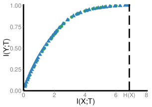
Figure 2: Example IB and DIB solutions. Left: IB plane. Right: DIB plane. Upper limit of the $y$-axes is $I\!\left(X,Y\right)$, since this is the maximal possible value of $I\!\left(T;Y\right)$. Upper limit of the $x$-axes is $\log\!\left(\left|T\right|\right)$, since this is the maximal possible value of $H\!\left(T\right)$ and $I\!\left(X,T\right)$ (the latter being true since $I\!\left(X,T\right)$ is bounded above by both $H\!\left(T\right)$ and $H\!\left(X\right)$, and $\left|T\right|<\left|X\right|$). The dashed vertical lines mark $H\!\left(X\right)$, which is both an upper bound for $I\!\left(X,T\right)$ and a natural comparison for $H\!\left(T\right)$ (since to place each data point in its own cluster, we need $H\!\left(T\right)=H\!\left(X\right)$).

To encourage the IB to perform closer to DIB optimality at small $\beta$, we next altered our initialization scheme of $q\!\left(t\mid x\right)$ to one biased towards single-cluster solutions; instead of each $x_{i}$ having most of its probability mass on a unique cluster $t_{i}$, we placed most of the probability mass for each $x_{i}$ on the same cluster $t^{*}$. The intended effect was to start the IB closer to solutions in which all data points were mapped to a single cluster. Results are shown in figure 3. Here, $p_{0}$ is the amount of probability mass placed on the cluster $t^{*}$, that is $q\!\left(t^{*}\mid x\right)=p_{0},\thinspace\thinspace\forall x$; the probability mass for the remaining $\left|T\right|-1$ clusters was again initialized to a normalized uniform random vector. “random” refers to an initialization which skips placing the $p_{0}$ mass and just initializes each $q\!\left(t\mid x_{i}\right)$ to a normalized uniform random vector.

We note several features. First, although we can see a gradual shift of the IB towards DIB-like behavior in the DIB plane as $p_{0}\rightarrow 1$, the IB solutions never quite reach the performance of DIB. Moreover, as $p_{0}\rightarrow 1$, the single-cluster initializations exhibit a phase transition in which, regardless of $\beta$, they “skip” over a sizable fraction of lower-$I\!\left(Y;T\right)$ solutions that are picked up by DIB. Third, even for higher-$I\!\left(Y;T\right)$ solutions, the single-cluster initializations seem to perform suboptimally, not quite extracting all of the information $I\!\left(X;Y\right)$, as DIB and the multi-cluster initialization from the previous section do; this can be seen in both the IB and DIB plane.

Figure 3: Example IB and DIB solutions across different IB initializations. Details identical to Figure 2, except colors represent different initializations for the IB, as described in the text.

To summarize, the IB and DIB perform similarly by the IB standards, but the DIB tends to outperform the IB dramatically by the DIB’s standards. Careful initialization of the IB can make up some of the difference, but not all.

It is also worth noting that, across all the datasets we tested, the DIB also tended to converge faster, as illustrated in figure 4. The DIB speedup over IB varied depended on the convergence conditions. In our experiments, we defined convergence as when the relative step-to-step change in the cost functional $L$ was smaller than some threshold ctol, that is when $\frac{L_{n-1}-L_{n}}{L_{n-1}}<\text{ctol}$ at step $n$. In the results above, we used $\text{ctol}=10^{-3}$. In figure 4, we vary ctol, with the IB initialization scheme fixed to the original “multi-cluster” version, to show the effect on the relative speedup of DIB over IB. While DIB remained $\approx$2-5x faster than IB in all cases tested, that speedup tended to be more pronounced with lower ctol. Since the ideal convergence conditions would probably vary by dataset size and complexity, it is difficult to make any general conclusions, though our experiments do at least suggest that DIB offers a computational advantage over IB.

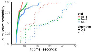
Figure 4: Fit times for IB and DIB. Cumulative distribution function of fit times across $\beta$, for a variety of settings of the convergence tolerance. Note that absolute numbers here depend on hardware, so we emphasize only relative comparisons of IB vs DIB. Note also that across the range of ctol values we tested here, the (D)IB curves vary by less than the width of the data points, and so we omit them.

5 Related work

The DIB is not the first hard clustering version of IB. Indeed, the agglomerative information bottleneck (AIB) [Slonim & Tishby (1999)] also produces hard clustering and was introduced soon after the IB. Thus, it is important to distinguish between the two approaches. AIB is a bottom-up, greedy method which starts with all data points belonging to their own clusters and iteratively merges clusters in a way which maximizes the gain in relevant information. It was explicitly designed to produce a hard clustering. DIB is a top-down method derived from a cost function that was not designed to produce a hard clustering. Our starting point was to alter the IB cost function to match the source coding notion of compression. The emergence of hard clustering in DIB is itself a result. Thus, while AIB does provide a hard clustering version of IB, DIB contributes the following in addition: 1) Our study emphasizes why a stochastic encoder is optimal for IB, namely due to the noise entropy term. 2) Our study provides a principled, top-down derivation of a hard clustering version of IB, based upon an intuitive change to the cost function. 3) Our non-trivial derivation also provides a cost function and solution which interpolates between DIB and IB, by adding back the noise entropy continuously, i.e. with $0<\alpha<1$. This interpolation may be viewed as adding a regularization term to DIB, one that may perhaps be useful in dealing with finitely sampled data. Another interpretation of the cost function with intermediate $\alpha$ is as a penalty on both the mutual information between $X$ and $T$ and the entropy of the compression, $H(T)$.

The original IB also provides a deterministic encoding upon taking the limit $\beta\rightarrow\infty$ that corresponds to the causal-state partition of histories [Still et al (2010)]. However, this is the limit of no compression, whereas our approach allows for an entire family of deterministic encoders with varying degrees of compression.

6 Discussion

Here we have introduced the deterministic information bottleneck (DIB) as an alternative to the information bottleneck (IB) for compression and clustering. We have argued that the DIB cost function better embodies the goal of lossy compression of relevant information, and shown that it leads to a non-trivial deterministic version of the IB. We have compared the DIB and IB solutions on synthetic data and found that, in our experiments, the DIB performs nearly identically to the IB in terms of the IB cost function, but far superior in terms of its own cost function. We also noted that the DIB achieved this performance at a computational efficiency 2-5x better than the IB.

Of course, in addition to the studies with synthetic data here, it is important to compare the DIB and IB on real world datasets as well to see whether the DIB’s apparent advantages hold, for example with datasets that have more explicit hierarchical structure for both algorthms to exploit, such as in topic modelling [Blei et al (2004), Slonim & Weiss (2002)].

One particular application of interest is maximally informative clustering, where it would be interesting to know how IB and DIB relate to classic clustering algorithms such as $k$-means [Strouse & Schwab (2017)]. Previous work has, for example, offered a principled way of choosing the number of clusters based on the finiteness of the data [Still & Bialek (2004)], and similarly interesting results may exist for the DIB. More generally, there are learning theory results showing generalization bounds on IB for which an analog on DIB would be interesting as well [Shamir et al (2010)].

Another potential area of application is modeling the extraction of predictive information in the brain (which is one particular example in a long line of work on the exploitation of environmental statistics by the brain [Barlow (1981), Barlow (2001), Barlow (2001), Atick & Redlich (1992), Olshausen & Field (1996), Olshausen & Field (1997), Simoncelli & Olshausen (2001), Olshausen & Field (2004)]). There, $X$ would be the stimulus at time $t$, $Y$ the stimulus a short time in the future $t+\tau$, and $T$ the activity of a population of sensory neurons. One could even consider neurons deeper in the brain by allowing $X$ and $Y$ to correspond not to an external stimulus, but to the activity of upstream neurons. An analysis of this nature using retinal data was recently performed with the IB [Palmer et al (2015)]. It would be interesting to see if the same data corresponds better to the behavior of the DIB, particularly in the DIB plane where the IB and DIB differ dramatically.

We close by noting that DIB is an imperfect name for the algorithm introduced here for a couple of reasons. First, there do exist other deterministic limits and approximations to the IB (see, for example, the discussion of the AIB in section 5), and so we hesitate to use the phrase “the” deterministic IB. Second, our motivation here was not to create a deterministic version of IB, but instead to alter the cost function in a way that better encapsulates the goals of certain problems in data analysis. Thus, the deterministic nature of the solution was a result, not a goal. For this reason, “entropic bottleneck” might also be an appropriate name.

7 Acknowledgements

For insightful discussions, we would like to thank Richard Turner, Máté Lengyel, Bill Bialek, Stephanie Palmer, and Gordon Berman. We would also like to acknowledge financial support from NIH K25 GM098875 (Schwab), the Hertz Foundation (Strouse), and the Department of Energy Computational Sciences Graduate Fellowship (Strouse).

8 Appendix: derivation of generalized IB solution

Given $p\!\left(x,y\right)$ and subject to the Markov constraint $T\leftrightarrow X\leftrightarrow Y$, the generalized IB problem is:

$$\min_{q\left(t|x\right)}L\!\left[q\!\left(t|x\right)\right] =H\!\left(T\right)-\alpha H\!\left(T|X\right)-\beta I\!\left(Y;T\right)-\sum_{x,t}\lambda\!\left(x\right)q\!\left(t|x\right),$$ (25)

where we have now included the Lagrange multiplier term (which enforces normalization of $q\!\left(t|x\right)$) explicitly. The Markov constraint implies the following factorizations:

$$q\!\left(t|y\right) =\sum_{x}q\!\left(t|x\right)p\!\left(x|y\right)$$ (26)

$$q\!\left(t\right) =\sum_{x}q\!\left(t|x\right)p\!\left(x\right),$$ (27)

which give us the following useful derivatives:

$$\frac{\delta q\!\left(t|y\right)}{\delta q\!\left(t|x\right)} =p\!\left(x|y\right)$$ (28)

$$\frac{\delta q\!\left(t\right)}{\delta q\!\left(t|x\right)} =p\!\left(x\right).$$ (29)

Now taking the derivative of the cost function with respect to the encoding distribution, we get:

$$\frac{\delta L}{\delta q\!\left(t|x\right)} =-\frac{\delta}{\delta q\!\left(t|x\right)}\sum_{t}q\!\left(t\right)\log q\!\left(t\right)-\frac{\delta}{\delta q\!\left(t|x\right)}\sum_{x,t}\lambda\!\left(x\right)q\!\left(t|x\right)$$ (30)

$$+\alpha\frac{\delta}{\delta q\!\left(t|x\right)}\sum_{x,t}q\!\left(t|x\right)p\!\left(x\right)\log q\!\left(t|x\right)$$ (31)

$$-\beta\frac{\delta}{\delta q\!\left(t|x\right)}\sum_{y,t}q\!\left(t|y\right)p\!\left(y\right)\log\!\left[\frac{q\!\left(t|y\right)}{q\!\left(t\right)}\right]$$ (32)

$$=-\log q\!\left(t\right)\frac{\delta q\!\left(t\right)}{\delta q\!\left(t|x\right)}-q\!\left(t\right)\frac{\delta\log q\!\left(t\right)}{\delta q\!\left(t|x\right)}-\lambda\!\left(x\right)\frac{\delta q\!\left(t|x\right)}{\delta q\!\left(t|x\right)}$$ (33)

$$+\alpha\left[p\!\left(x\right)\log q\!\left(t|x\right)\frac{\delta q\!\left(t|x\right)}{\delta q\!\left(t|x\right)}+q\!\left(t|x\right)p\!\left(x\right)\frac{\delta\log q\!\left(t|x\right)}{\delta q\!\left(t|x\right)}\right]$$ (34)

$$-\beta\sum_{y}\left[p\!\left(y\right)\log\!\left[\frac{q\!\left(t|y\right)}{q\!\left(t\right)}\right]\frac{\delta q\!\left(t|y\right)}{\delta q\!\left(t|x\right)}\right]$$ (35)

$$+\beta\sum_{y}\left[q\!\left(t|y\right)p\!\left(y\right)\frac{\delta\log q\!\left(t|y\right)}{\delta q\!\left(t|x\right)}+q\!\left(t|y\right)p\!\left(y\right)\frac{\delta\log q\!\left(t\right)}{\delta q\!\left(t|x\right)}\right]$$ (36)

$$=-p\!\left(x\right)\log q\!\left(t\right)-p\!\left(x\right)-\lambda\!\left(x\right)+\alpha\left[p\!\left(x\right)\log q\!\left(t|x\right)+p\!\left(x\right)\right]$$ (37)

$$-\beta\sum_{y}\left[p\!\left(y\right)\log\!\left[\frac{q\!\left(t|y\right)}{q\!\left(t\right)}\right]p\!\left(x|y\right)+p\!\left(y\right)p\!\left(x|y\right)-q\!\left(t|y\right)p\!\left(y\right)\frac{p\!\left(x\right)}{q\!\left(t\right)}\right]$$ (38)

$$=-p\!\left(x\right)\log q\!\left(t\right)-p\!\left(x\right)-\lambda\!\left(x\right)+\alpha\left[p\!\left(x\right)\log q\!\left(t|x\right)+p\!\left(x\right)\right]$$ (39)

$$-\beta p\!\left(x\right)\left[\sum_{y}p\!\left(y|x\right)\log\!\left[\frac{q\!\left(t|y\right)}{q\!\left(t\right)}\right]+\sum_{y}p\!\left(y|x\right)-\sum_{y}q\!\left(y|t\right)\right]$$ (40)

$$=p\!\left(x\right)\left[-1-\log q\!\left(t\right)-\frac{\lambda\!\left(x\right)}{p\!\left(x\right)}+\alpha\log q\!\left(t|x\right)+\alpha-\beta\left[\sum_{y}p\!\left(y|x\right)\log\!\left[\frac{q\!\left(t|y\right)}{q\!\left(t\right)}\right]\right]\right].$$ (41)

Setting this to zero implies that:

$$\alpha\log q\!\left(t|x\right) =1-\alpha+\log q\!\left(t\right)+\frac{\lambda\!\left(x\right)}{p\!\left(x\right)}+\beta\left[\sum_{y}p\!\left(y|x\right)\log\!\left[\frac{q\!\left(t|y\right)}{q\!\left(t\right)}\right]\right].$$ (42)

We want to rewrite the $\beta$ term as a KL divergence. First, we will need that $\log\!\left[\frac{q\left(t|y\right)}{q\left(t\right)}\right]=\log\!\left[\frac{q\left(t,y\right)}{q\left(t\right)p\left(y\right)}\right]=\log\!\left[\frac{q\left(y|t\right)}{p\left(y\right)}\right]$. Second, we will add and subtract $\beta\sum_{y}p\!\left(y|x\right)\log\!\left[\frac{p\left(y|x\right)}{p\left(y\right)}\right]$. This gives us:

$$\alpha\log q\!\left(t|x\right) =1-\alpha+\log q\!\left(t\right)+\frac{\lambda\!\left(x\right)}{p\!\left(x\right)}+\beta\sum_{y}p\!\left(y|x\right)\log\!\left[\frac{p\!\left(y|x\right)}{p\!\left(y\right)}\right]$$ (43)

$$-\beta\left[\sum_{y}p\!\left(y|x\right)\log\!\left[\frac{p\!\left(y|x\right)}{q\!\left(y|t\right)}\right]\right].$$ (44)

The second $\beta$ term is now just $D_{\text{KL}}\!\left[p\!\left(y|x\right)\mid q\!\left(y|t\right)\right]$. Dividing both sides by $\alpha$, this leaves us with the equation:

$$\log q\!\left(t|x\right) =z\!\left(x,\alpha,\beta\right)+\frac{1}{\alpha}\log q\!\left(t\right)-\frac{\beta}{\alpha}D_{\text{KL}}\!\left[p\!\left(y\mid x\right)|q\!\left(y|t\right)\right],$$ (45)

where we have absorbed all of the terms that don’t depend on $t$ into a single factor:

$$z\!\left(x,\alpha,\beta\right) \equiv\frac{1}{\alpha}-1+\frac{\lambda\!\left(x\right)}{\alpha p\!\left(x\right)}+\frac{\beta}{\alpha}\sum_{y}p\!\left(y\mid x\right)\log\!\left[\frac{p\!\left(y\mid x\right)}{p\!\left(y\right)}\right].$$ (46)

Solving for $q\!\left(t|x\right)$, we get:

$$q\!\left(t|x\right) =\exp\!\left[z\right]\exp\!\left[\frac{1}{\alpha}\left(\log q\!\left(t\right)-\beta D_{\text{KL}}\!\left[p\!\left(y|x\right)\mid q\!\left(y|t\right)\right]\right)\right]$$ (47)

$$=\frac{1}{Z}\exp\!\left[\frac{1}{\alpha}\left(\log q\!\left(t\right)-\beta D_{\text{KL}}\!\left[p\!\left(y|x\right)\mid q\!\left(y|t\right)\right]\right)\right],$$ (48)

where:

$$Z\!\left(x,\alpha,\beta\right) \equiv\exp\!\left[-z\right]$$ (49)

is just a normalization factor. Now that we’re done with the general derivation, let’s add a subscript to the solution to distinguish it from the special cases of the IB and DIB.

$$q_{\alpha}\!\left(t|x\right) =\frac{1}{Z\!\left(x,\alpha,\beta\right)}\exp\!\left[\frac{1}{\alpha}\left(\log q\!\left(t\right)-\beta D_{\text{KL}}\!\left[p\!\left(y|x\right)\mid q\!\left(y|t\right)\right]\right)\right].$$ (50)

The IB solution is then:

$$q_{\text{IB}}\!\left(t|x\right)=q_{\alpha=1}\!\left(t|x\right) =\frac{q\!\left(t\right)}{Z}\exp\!\left[-\beta D_{\text{KL}}\!\left[p\!\left(y|x\right)\mid q\!\left(y|t\right)\right]\right],$$ (51)

while the DIB solution is:

$$q_{\text{DIB}}\!\left(t|x\right)=\lim_{\alpha\rightarrow 0}q_{\alpha}\!\left(t|x\right) =\delta\!\left(t-t^{*}\!\left(x\right)\right),$$ (52)

with:

$$t^{*}\!\left(x\right) =\text{$\underset{t}{\operatorname{argmax}}$}\left(\log q\!\left(t\right)-\beta D_{\text{KL}}\!\left[p\!\left(y|x\right)\mid q\!\left(y|t\right)\right]\right).$$ (53)

References

- Atick & Redlich (1992) Atick, J.J. & Redlich, A.N. (1992). What Does the Retina Know about Natural Scenes? Neural Computation, 4, 196-210.
- Bach & Jordan (2005) Bach, F.R., & Jordan, M.I. (2005). A probabilistic interpretation of canonical correlation analysis. Technical Report.
- Barlow (1981) Barlow, H.B. (1981). Critical Limiting Factors in the Design of the Eye and Visual Cortex. Proceedings of the Royal Society B: Biological Sciences, 212(1186), 1–34.
- Barlow (2001) Barlow, H. (2001). Redundancy reduction revisited. Network: Computation in Neural Systems, 12(3), 241–253.
- Barlow (2001) Barlow, H. (2001). The exploitation of regularities in the environment by the brain. Behav. Brain Sci. 24, 602–607.
- Bekkerman et al (2001) Bekkerman, R., El-Yaniv, R., Tishby, N., & Winter, Y. (2001). On feature distributional clustering for text categorization. Proceedings of SIGIR-2001.
- Bekkerman et al (2003) Bekkerman, R., El-Yaniv, R., & Tishby, N. (2003). Distributional word clusters vs. words for text categorization. Journal of Machine Learning Research, 3, 1183-1208.
- Blei et al (2004) Blei, D.M., Griffiths, T.L., Jordan, M.I. & Tenenbaum, J.B. (2004). Hierarchical Topic Models and the Nested Chinese Restaurant Process. Proc. of Advances in Neural Information Processing System (NIPS).
- Chechik et al (2005) Chechik, G., Globerson, A., Tishby, N., & Weiss, Y. (2005). Information Bottleneck for Gaussian Variables. Proc. of Advances in Neural Information Processing System (NIPS).
- Cover & Thomas (2006) Cover, T.M. & Thomas, J.A. (2006). Elements of Information Theory. John Wiley & Sons, Inc.
- Creutzig et al (2009) Creutzig, F., Globerson, A., & Tishby, N. (2009). Past-future information bottleneck in dynamical systems. Physical Review E, 79(4).
- Hecht & Tishby (2005) Hecht, R.M. & Tishby, N. (2005). Extraction of relevant speech features using the information bottleneck method. InterSpeech.
- Hecht & Tishby (2008) Hecht, R.M. & Tishby, N. (2007). Extraction of relevant Information using the Information Bottleneck Method for Speaker Recognition. InterSpeech.
- Hecht et al (2009) Hecht, R.M., Noor, E., & Tishby, N. (2009). Speaker recognition by Gaussian information bottleneck. InterSpeech.
- Kandel et al (2000) Kandel, E.R., Schwartz, J.H., Jessell, T.M., Siegelbaum, S.A., & Hudspeth, A.J. (2013). Principles of neural science (5th ed.). New York: McGraw-Hill, Health Professions Division.
- Kinney & Atwal (2014) Kinney, J.B. & Atwal, G.S. (2014). Equitability, mutual information, and the maximal information coefficient. PNAS.
- MacKay (2002) Mackay, D. (2002). Information Theory, Inference, & Learning Algorithms. Cambridge University Press.
- Olshausen & Field (1996) Olshausen, B.A., & Field, D.J. (1996). Emergence of simple-cell receptive field properties by learning a sparse code for natural images. Nature, 381(6583), 607–609.
- Olshausen & Field (1997) Olshausen, B.A., & Field, D.J. (1997). Sparse coding with an overcomplete basis set: A strategy employed by V1? Vision Research.
- Olshausen & Field (2004) Olshausen, B.A., & Field, D.J. (2004). Sparse coding of sensory inputs. Current Opinion in Neurobiology, 14(4), 481–487.
- Palmer et al (2015) Palmer, S.E., Marre, O., Berry, M.J., & Bialek, W. (2015). Predictive information in a sensory population. PNAS, 112(22), 6908–6913.
- Schneidman et al (2002) Schneidman, E., Slonim, N., Tishby, N., deRuyter van Steveninck, R., & Bialek, W. (2002). Analyzing neural codes using the information bottleneck method. Proc. of Advances in Neural Information Processing System (NIPS).
- Shamir et al (2010) Shamir, O., Sabato, S., & Tishby, N. (2010). Learning and Generalization with the Information Bottleneck. Theoretical Computer Science, Volume 411, Issues 29-30, Pages 2696-2711.
- Simoncelli & Olshausen (2001) Simoncelli, E.P., & Olshausen, B.A. (2001). Natural image statistics and neural representation. Annual Review of Neuroscience.
- Slonim & Tishby (1999) Slonim, N., & Tishby, N. (1999). Agglomerative information bottleneck. Proc. of Advances in Neural Information Processing System (NIPS).
- Slonim & Tishby (2000) Slonim, N., & Tishby, N. (2000). Document clustering using word clusters via the information bottleneck method. Proceedings of the 23rd Annual International ACM SIGIR Conference on Research and Development in Information Retrieval, 208–215.
- Slonim & Tishby (2001) Slonim, N., & Tishby, N. (2001). The Power of Word Clusters for Text Classification. Proceedings of the European Colloquium on IR Research, ECIR 2001, 1–12.
- Slonim & Weiss (2002) Slonim, N., & Weiss, Y. (2002). Maximum likelihood and the information bottleneck. Proc. of Advances in Neural Information Processing System (NIPS), 15, 335–342.
- Still & Bialek (2004) Still, S., & Bialek, W. (2004). How many clusters? An information-theoretic perspective. Neural Computation, 16(12), 2483–2506.
- Still et al (2010) Still, S., Crutchfield, J.P., & Ellison, C.J. (2010). Optimal causal inference: Estimating stored information and approximating causal architecture. Chaos: an Interdisciplinary Journal of Nonlinear Science, 20(3), 037111.
- Strouse & Schwab (2017) Strouse, DJ & Schwab, D. (2017). On the relationship between distributional and geometric clustering. In progress.
- Tishby (1999) Tishby, N., Pereira, F. & Bialek, W. (1999). The Information Bottleneck Method. Proceedings of The 37th Allerton Conference on Communication, Control, & Computing, Univ. of Illinois.
- Tishby & Zaslavsky (2015) Tishby, N., & Zaslavsky, N. (2015). Deep Learning and the Information Bottleneck Principle. arXiv.org.
- Turner & Sahani (2007) Turner, R.E., & Sahani, M. (2007). A maximum-likelihood interpretation for slow feature analysis. Neural Computation, 19(4), 1022–1038.
- Wallace (1991) Wallace, G.K. (1991). The JPEG Still Picture Compression Standard. Commun. ACM, vol. 34, pp. 30-44.