Half-Duplex or Full-Duplex Communications: Degrees of Freedom Analysis under Self-Interference

Abstract

In-band full-duplex (FD) communication provides a promising alternative to half-duplex (HD) for wireless systems, due to increased spectral efficiency and capacity. In this paper, HD and FD radio implementations of two way, two hop and two way two hop communication are compared in terms of degrees of freedom (DoF) under a realistic residual self-interference (SI) model. DoF analysis is carried out for each communication scenario for HD, antenna conserved (AC) and RF chain conserved (RC) FD radio implementations. The DoF analysis indicates that for the two way channel, the achievable AC FD with imperfect SI cancellation performs strictly below HD, and RC FD DoF trade-off is superior when the SI can be sufficiently cancelled. For the two hop channel, FD is better when the relay has large number of antennas and enough SI cancellation. For the two way two hop channel, when both nodes require similar throughput, the achievable DoF pairs for FD do not outperform HD. FD still can achieve better DoF pairs than HD, provided the relay has sufficient number of antennas and SI suppression.

I Introduction

In almost all networks, a communicating device has a dual task of reception and transmission of data. This is commonly achieved via half-duplex (HD) operation, where the channel is time shared between transmission and reception, so that a node can either transmit or receive at a given time. Full-duplex (FD) operation provides a promising alternative, where both of these activities are implemented simultaneously. However, an FD node suffers from high amount of self-interference (SI), since typically the transmitted signal is about 100 dB stronger than the received signal. Recently FD has gained considerable interest due to promising results on practical implementations [2, 3, 4, 5, 6], as can be seen in the recent review article [7] and references therein.

Ideally, FD implementation uses the channel for transmitting and receiving simultaneously, and hence it is likely to give higher throughput. On the other hand, FD requires hardware resources, such as antennas to be divided between transmission and reception, in order to accomplish this with as little SI as possible. However, since SI cannot be suppressed completely, the residual SI reduces the received signal-to-interference-noise ratio (SINR), resulting in reduced data rates. Hence, how much improvement can FD communication in the presence of SI can provide over HD, considering similar hardware resources is an important question that needs to be investigated thoroughly for viability of FD. In order to address this problem, in this paper we compare wireless HD and FD communication in three communication scenarios, two way, two hop (relaying), and two way two hop (two way relaying) systems, illustrated in Figures 1-4, from degrees of freedom (DoF) point of view. The system models considered in this paper arise naturally in modern communication scenarios, such as cellular, WiFi, mesh or ad-hoc networks, which would particularly benefit from FD implementations.

One of the challenges in analytical study of the FD systems is the modeling of the residual SI. The model should be accurate, so that it captures the effect of SI, and also simple enough, so that it is useful for analysis and design. Some works assume constant increase in the noise floor due to SI [8, 6]. However, it is reasonable to expect that SI will depend on the transmit power. Other works assume linear increase in SI with transmit power [9, 10, 11], but this model fails to capture the effect, in which increased transmission power actually enhances SI suppression, since a better estimate of the SI signal is obtained. In our analysis in this paper, we use the experimentally validated SI model from [12], which shows that average residual SI power after cancellation can be modeled as proportional to $P^{1-\lambda}$, where $0\leq\lambda\leq 1$ is a constant that depends on the transceiver’s ability to mitigate SI and $P$ is the transmit power. This model, also used in [13], not only captures the effect of the practical SI cancellation mechanisms employed, but it is analytically tractable as well. Furthermore, it generalizes all other models used in the literature.

In order to provide a fair comparison of FD and HD implementations, it is important to keep the hardware resources fixed. For this purpose, we follow two approaches as in [14]: For each node, we either keep the total number of antennas or we keep the total number of RF chains of FD mode the same as that of HD mode, considering antenna conserved (AC) and RF chain conserved (RC) implementations of FD, respectively. The AC FD scenario is motivated by the recent FD implementations [2, 6]; the notion of keeping the number of RF chains equal is also reasonable from a practical perspective, since RF chains are the components that dominantly increase the total cost of a radio [15].

In this paper, considering the three scenarios, namely two way, two hop and two way two hop communication, under realistic SI and hardware constraints, we pursue the high-SNR DoF analysis [16] for comparison of the performances of HD and FD modes. The DoF metric admits simple analytical characterization facilitating the comparisons. Our analysis in this paper not only provides the guidelines for selection of HD or FD mode for the considered scenarios, but it also sets forth the basic models for future studies for more complex scenarios. Our main observations can be summarized as follows:

• For the two way channel (Figure 1), we show that in presence of SI ($\lambda<1$), the FD DoF region, which shows the simultaneously achievable DoF pairs by both users for the AC scenario lies strictly inside the HD trade-off. For the RC scenario, however, with “good” SI suppression (typically $\lambda>0.75$), FD can achieve certain DoF pairs which are not achievable by the HD implementation.

• For the two hop channel (a relay channel without a direct link between the source and destination) as shown in Figure 2, we compare the FD and HD DoFs for the symmetric case (when both source and destination have equal number of antennas) and the asymmetric case (when source has a single antenna, and destination has multiple antennas). We find that, for given number of source and destination antennas, and SI parameter $\lambda$, the FD implementation outperforms HD if the relay has sufficient number of antennas, otherwise HD is better. Number of antennas required at the relay for this crossover is lower for the RC scenario, than that of the AC scenario, and depends on the SI mitigation level $\lambda$ and the number of source and destination antennas. When the number of antennas at each node is fixed, then there exists threshold value of $\lambda$, below which HD achieves higher throughput than FD.

• For the two way two hop channel (two way relay channel without a direct link between the communicating nodes, as shown in Figures 3 and 4), with only the relay having FD capability, in both AC and RC scenarios, if the symmetric DoF is to be maximized, then generally HD performs better than FD. For the asymmetric case however, provided the SI suppression is high enough (in terms of $\lambda$), FD can achieve certain DoF pairs which are not achievable by the HD. These pairs generally correspond to the extreme asymmetric DoF, when one node’s DoF requirement is significantly higher than the other one.

I-A Related Literature

Recently, there has been a significant body of work on FD communications, and here, we briefly summarize the most relevant papers. In [17], the achievable sum rates in a two way channel for FD and HD are compared assuming perfect SI cancellation for AC implementation. Reference [18] compares the FD and HD two way channel in the presence of channel estimation errors, and depending on the level of SI and the channel estimation errors, an outer bound for the region over which FD is better than HD is provided. An outage analysis for FD two way communication under fading can be found in [19]. In [20], results on the sum rate performance of two way HD and FD communication are presented considering the FD implementations from [14], which are optimistic for the RC FD implementation with larger number of antennas. In [21], a study on FD Multiple Input Multiple Output (MIMO) system is presented, basically showing how a common carrier based FD radio with a single antenna, as in [3], can be transformed into a common carrier FD MIMO radio.

In [22], two hop communication is studied with channel estimation errors in the presence of loop-back interference in order to come up with capacity cut-set bounds for both HD and FD relaying. An effective transmission power policy is proposed for the relay to maximize this bound, and performance of FD relaying with optimal power control is compared with HD relaying. Two hop communication in a cellular environment is investigated in [23], where a hybrid scheduler that is capable of switching between HD and FD in an opportunistic fashion is proposed, for maximizing the system throughput. Reference [10] has shown that, in order to control the SI, the relay should employ power control and the proposed relaying scheme allows to switch between HD and FD modes in an opportunistic fashion, while transmit power is adjusted to maximize spectral efficiency. In [1], results in the relaying scenario are presented, comparing FD and HD relaying under the empirical residual SI model from [12]. In that work, power control is used asymptotically, so that the relay scales its power with respect to the source to achieve maximum DoF, when the relay operates in decode and forward mode. Similar asymptotic power control was also observed to give higher DoF in amplify and forward in mode in [13]. In [24], two way relaying HD and FD systems are analyzed, where source and destination nodes are assumed to hear each other. A survey on FD relaying can be found in [25].

The current literature does not contain a detailed investigation of the DoF analysis for the three communication scenarios under realistic SI and hardware constraints, as considered in this paper. In most of the existing literature, a specific self-interference (SI) model is used, and the HD and FD performance is compared for that SI model. Furthermore, the SI model used either assumes SI power scales linearly with transmit power, or SI is taken simply as an increase in the noise floor. In this paper, we use a generalized and experimentally validated SI model that incorporates and generalizes both scenarios and compare the HD and FD performance. We study the DoF of three important building blocks of a wireless network: two way communication, single hop and two way two hop. These channel models and the analysis illustrate the fundamental benefits and limitations of using FD in typical wireless scenarios.

I-B Paper Organization

The rest of the paper is organized as follows: Section II describes the considered three system models for two way, two hop and two way two hop communication, together with channel, FD implementation and SI cancellation models. In Sections III-V, the DoF analysis is presented with detailed comparisons and discussions of the HD and FD implementations of the three system models. Section VI involves our concluding remarks.

II System Models

In the following, we describe the three different scenarios, two way, two hop and two way two hop communication, in which FD can be implemented. We start by providing a wireless channel model between two nodes, as a generalized point-to-point channel model that will be used throughout the paper. Then, for each communication model, we present the information flow for both HD and FD implementations.

II-A Generic Channel Model Between Two Nodes

Consider a scenario where node $A$ is transmitting to node $B$, where node $B$ is operating either in HD mode or FD mode depending upon scenario being investigated. Let $P_{A}$ denote the average transmit power at node $A$, $\sigma_{B}^{2}$ is the average power of the AWGN at node $B$. Nodes are assumed to have multiple antennas with $\mathbf{H}_{AB}$ denoting the channel matrix between nodes $A$ and $B$. We assume Rayleigh fading channel, so the entries of $\mathbf{H}_{AB}$ are taken as independent and identically distributed circularly symmetric complex Gaussian random variables with unit variance [26]. Channel state information is assumed to be available only at the receiver. The size of the channel matrices depends on the number of the transmit and receive antennas employed at the nodes. Then, the received signals at node $B$ is

$$\mathbf{y}_{B} =\frac{1}{\sqrt{K}}\mathbf{H}_{AB}\mathbf{x}_{A}+\mathbf{w}_{B}+\mathbf{i}_{B}.$$

Here, $\mathbf{x}_{A}$ denotes the vector of the transmitted symbol, $\mathbf{w}_{B}$ denotes the noise term, and $\mathbf{i}_{B}$ is the SI term if node $B$ is operating in FD mode. We assume entries of $\mathbf{i}_{B}$ are Gaussian distributed with variance equal to average SI power. This assumption makes analysis tractable and can be viewed as the worst case scenario, since Gaussian distribution gives worst case capacity [27, 28]. Clearly, in the case of HD, this term is set to zero. Expected value of $i_{B}$ will be denoted as $I_{B}$. Finally, $K$ is the parameter that characterizes the path loss between nodes. The SINR at the receiver is,

$$\Gamma_{AB}=\frac{P_{A}}{K\left(\sigma_{B}^{2}+I_{B}(P_{B})\right)},$$ (1)

where we have explicitly showed the dependence of the average SI, $I_{B}$ on $P_{B}$, the transmit power of $B$ according to [12]. Details of the SI model will be described in Section II-C. Then, assuming that node $A$ transmits using $N_{A}$ antennas and node $B$ receives using $N_{B}$ antennas, the average achievable rate $R_{AB}$ is [16]

$$R_{AB}=\mathbb{E}\left[\log\det\left(\mathbf{I}+\frac{\Gamma_{AB}}{N_{A}}\mathbf{H}_{AB}\mathbf{H}_{AB}^{*}\right)\right].$$

Degrees of Freedom (DoF) analysis characterizes the achievable rate at high SNR. For a point to point MIMO AWGN Rayleigh fading channel with $N_{A}$ antennas at $A$ and $N_{B}$ antennas at $B$, the largest DoF is given by[16]

$$\text{DoF}_{AB}=\lim_{P_{A}\to\infty}\frac{R_{AB}}{\log(P_{A})}=\min\left(N_{B},N_{A}\right).$$

II-B Communication Scenarios

II-B1 Two Way Channel

Two way communication channel was introduced by Shannon in [29]. Here, we consider a two way wireless channel, where node $A$ and $B$ have $N_{A}$ and $N_{B}$ antennas respectively, and wish to communicate with one another. This channel, for example may model a WiFi router communicating with a wireless device, which is simultaneously uploading and downloading data. In the HD mode, the nodes time share the wireless medium, taking turns transmitting as shown in Figures 1(a) and 1(b). In this case, nodes use all of their antennas either for transmission or for reception. If both $A$ and $B$ are FD capable, then they can use the channel simultaneously for transmission and reception, as shown in Figure 1(c). Here, $t_{A}$ and $r_{A}$ denote the number of transmit and receive antennas at node $A$, respectively. Similarly, $t_{B}$ and $r_{B}$ denote the number of antennas at node $B$. Dotted arrows in each direction represent the SI channels. The choice of $t_{A},r_{A},t_{B}$ and $r_{B}$ based on hardware constraints will be discussed in Section II-D.

(a) HD communication with $A$ transmitting to $B$

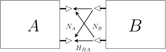
(b) HD communication with $B$ transmitting to $A$

(c) FD communication, dotted arrows indicate SI.

Figure 1: Two way channel

II-B2 Two Hop Channel

In this scenario, node $A$ communicates with node $B$ through a relay node, $R$. We assume that there is no direct link between nodes $A$ and $B$, hence the relay assists in forwarding the packets from $A$ to $B$. The relay is assumed to operate according to decode and forward protocol, [30]. Nodes $A$ and $B$ have $N_{A}$ and $N_{B}$ antennas, respectively. Total number antennas employed in $R$ in the HD mode is denoted by $N_{R}$. When the relay operates in FD mode, then $t$ and $r$ denote the number of transmit and receive antennas respectively.

When the relay is in HD mode, the information flow takes place in two phases: First, $A$ transmits to $R$ as shown in Figure 2(a), and then $R$ decodes the packets and forwards to $B$, as shown in Figure 2(b). In the case of FD relaying, $R$ can receive from $A$ and simultaneously transmit to $B$, as shown in Figure2(c). It allocates its resources (antennas or RF chains) so as to increase the data rate from $A$ to $B$.

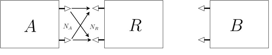
(a) First phase of HD relaying with $A$ transmitting to $R$

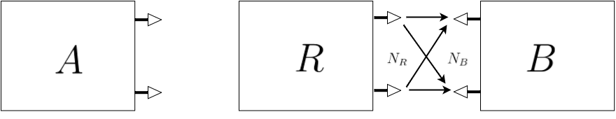
(b) Second phase of HD relaying with $R$ transmitting to $B$

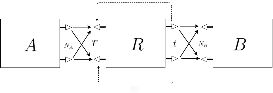
(c) FD relaying with $A$ transmitting to $R$, and $R$ transmitting to $B$,
dotted arrows indicate SI

Figure 2: Two hop channel

II-B3 Two Way Two Hop Channel

This channel models a two way relay channel without a direct link between communicating nodes. Here, two nodes $A$ (with $N_{A}$ antennas) and $B$ (with $N_{B}$ antennas) wish to communicate with each other through a relay $R$ (with $N_{R}$ antennas in HD mode). Only $R$ is assumed to have FD capability and uses $t$ antenna for transmission and $r$ antenna for reception in FD mode. A motivating example for such scenario is two stations on earth communicating via a satellite, with no direct link between the stations.

When $R$ is operated in HD mode, we consider an effective communication strategy, such as [31, 32, 33], which takes place in two phases, as shown in Figures 3(a) and 3(b). During the first phase, also known as the multiple access (MAC) phase, nodes $A$ and $B$ simultaneously transmit to $R$. During second phase, called broadcast (BC) phase, $R$ simultaneously transmits to $A$ and $B$, and both nodes can extract their desired signal by the virtue of analog coding techniques.

For the FD case, only $R$ is assumed to have FD capability, and two way FD communication occurs in two phases, as shown in Figures 4(a) and 4(b). During the first phase node $A$ transmits to $B$ via $R$, and since $R$ is FD, it can receive from node $A$ and transmit simultaneously to $B$. During the second phase, direction of information flow is reversed, as node $B$ transmits to $A$ via $R$.

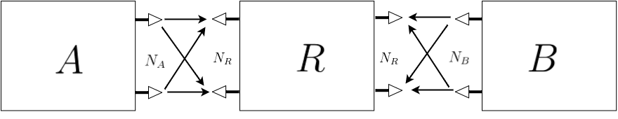
(a) MAC phase, nodes $A$ and $B$ transmitting to $R$

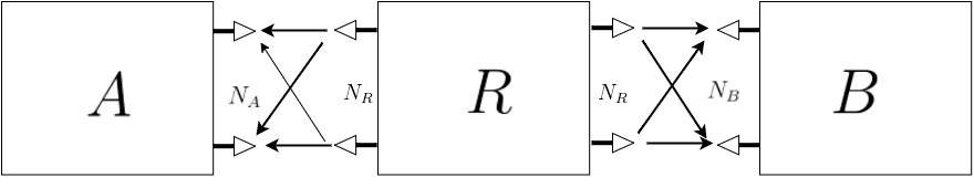
(b) BC phase, $R$ transmitting to $A$ and $B$

Figure 3: HD two way two hop channel

(a) First phase, $A$ transmitting to $R$, $R$ transmitting to $B$

(b) Second phase, $B$ transmitting to $R$, $R$ transmitting to $A$

Figure 4: FD two way two hop channel, dotted arrows indicate SI

II-C SI Cancellation Model

The major challenge of FD communication is SI cancellation. As discussed in detail in [34], the simplest SI cancellation technique is the passive one, obtained by the path-loss due to the separation between the transmit and receive antennas. More sophisticated active techniques, namely, analog cancellation and digital cancellation reduce the self-interference further. In analog cancellation, the FD node uses additional RF chains to estimate the channel between the transmitting and receiving antennas and then to subtract the interfering signal at the RF stage. In the digital cancellation, the self-interference is estimated and canceled in the baseband. Despite consecutive application of these three cancellation techniques, SI cannot be completely eliminated. In [12], the average power of the residual SI is experimentally modeled as

$${I}=\frac{P_{T}^{\left(1-\lambda\right)}}{\beta\mu^{\lambda}}.$$ (2)

Here, $P_{T}$ denotes the transmission power of the FD node. $\beta$, $\mu$, and $\lambda$ are the system parameters which depend on the cancellation technique employed, with $0\leq\lambda\leq 1$. Note that, $\lambda=1$ corresponds to increased noise floor SI model used in the literature and $\lambda=0$ corresponds to SI power scaling linearly with the transmit power.

This SI model was obtained for a FD transmitter with a single receive and single transmit antenna. In the case of a multiple transmit and receive antenna FD terminal, we could implement transmit precoding and receive processing to further mitigate the SI. At each receive antenna, this would at most increase $P_{T}$ in (2) by a factor of $t$ (number of transmit antennas), which for the purpose of a DoF analysis, would have the same effect as (2). Hence in this paper we continue to use (2) to model the average residual SI power per receive antenna.

A natural question then arises: can DoF can be improved by using such transmit and linear precoding and receive processing? In other words, is a DoF analysis based on the model in (2) unnecessarily pessimistic? We believe that is not the case since the SI channel matrix is generally full rank [35]. As reported in [36], unless the transmission is carried out in the null space of the SI channel, the SI power continues to scale with transmit power $P_{T}$, leading to the model in (2) for the purposes of a DoF analysis. On the other hand, if the encoder attempts to transmit in the null-space of the SI channel matrix, it would lead to loss in DoF since the SI matrix is full rank. Moreover, any such strategy would require very accurate estimates of the SI channel. We illustrate this for the case of the two way channel in Section III-C, where we show that in obtaining the DoF, the model in (2) is sufficient. Another advantage of the model in (2) is that it simply defers all SI mitigation to hardware and does not use any SI channel knowledge or SI management strategy while designing the transmit signal. We must add, however, that obtaining converse results, which show that no multi-antenna processing would improve the DoFs beyond the ones obtained in this paper, is reasonably arduous, as the SI is in general non-Gaussian.

II-D Hardware Resources in HD and FD

For a fair comparison of HD and FD communications, hardware resources must be equalized. We investigate two conservation scenarios: antenna conservation, where the number of antennas is kept equal, and RF chain conservation, where the number of RF chains is kept equal [14]. For instance, if a node has $N$ antennas in HD mode, then it would have total $2N$ RF chains ($N$ each for up-converting and down-converting). While considering AC FD, we take total number of antennas to be $N$, i.e., if $r$ antennas are used for reception then remaining $(N-r)$ antennas are used for transmission. Whereas for the RC FD implementation, the total number of RF chains is kept same as that in HD case, which is $2N$. Hence if $r$ antennas are used for reception, then in addition to $r$ down-converting RF chains, $r$ RF chains are used in analog cancellation, and remaining $2N-2r$ RF chains can be used for up-converting in transmission, resulting in $2N-2r$ transmit antennas. Note that, RC FD increases the total number of antennas in the FD mode. This is illustrated in Figure 5, where we consider a HD node with two antennas ($N=2$), and hence it has four RF chains (Figure 5(a)). In RC FD implementation, the total number of RF chains is four, resulting in two transmit and one receive antennas, since one RF chain is required for the analog cancellation (Figure 5(b)). In AC FD scenario there are two antennas, one each for transmission and reception (Figure 5(c)).

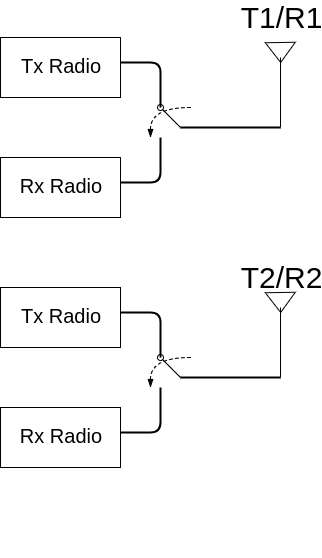
(a) HD node with two transmit and two receive antennas, and four RF chains

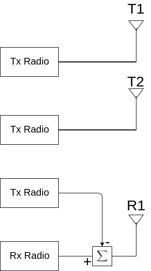
(b) RC FD node with two transmit and one receive antennas, and four RF chains

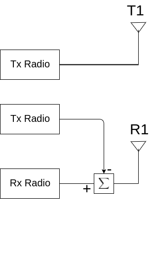
(c) AC FD node with one transmit and one receive antennas, and three RF chains

Figure 5: Illustration of HD, AC FD and RC FD implementations

Comparison of the number of antennas is summarized in Table I. (See also [14, 15].)

	number of RX	number of TX	Total number of
	antennas	antennas	antennas
HD	N	N	N
AC FD	r	N-r	N
RC FD	r	2N-2r	2N-r

TABLE I: Number of antennas in HD, AC FD and RC FD implementations

III Two Way Channel

As the first scenario, we consider two way channel between nodes $A$ and $B$, as illustrated in Figure 1. In this section, we formulate, calculate and compare the DoF of two way communication in HD and FD modes.

III-A Half-Duplex Mode

When nodes $A$ and $B$ communicate in HD mode in the same band, they need to employ time sharing. Hence, the nodes alternate for transmission, as depicted in Figures 1(a) and 1(b). Defining $\tau$ as the fraction of time, in which node $A$ transmits while node $B$ receives, the remaining fraction, $\left(1-\tau\right)$ is utilized by node $B$ for transmission while node $A$ receives.

III-A1 Achievable Rate

Recalling that the SINR at node $B$, $\Gamma_{AB}$ is calculated via equation (1), with the SI term $I_{B}(P_{B})$ as zero in HD mode, the average achievable rate from $A$ to $B$ $R^{HD}_{AB}$ can be obtained as [16],

$$R^{HD}_{AB}=\tau\mathbb{E}\left[\log\det\left(\mathbf{I}+\frac{\Gamma_{AB}}{N_{A}}\mathbf{H}_{AB}\mathbf{H}_{AB}^{*}\right)\right],$$ (3)

$$R^{HD}_{BA}=\left(1-\tau\right)\mathbb{E}\left[\log\det\left(\mathbf{I}+\frac{\Gamma_{BA}}{N_{B}}\mathbf{H}_{BA}\mathbf{H}_{BA}^{*}\right)\right],$$ (4)

where $\mathbf{I}$ denotes the identity matrix, with $\mathbf{I}\in\mathcal{C}^{N_{B}\times N_{B}}$ for (3) and $\mathbf{I}\in\mathcal{C}^{N_{A}\times N_{A}}$ for (4), and $N_{X}$ is the total number of antennas for node $X$.

III-A2 Degrees of Freedom

The DoF characterizing the performance at high SNR, for the two way channel considering HD communication is obtained as follows:

$$\text{DoF}^{HD}_{AB} =\lim_{P_{A}\to\infty}\frac{R_{AB}^{HD}}{\log(P_{A})}=\tau\min(N_{A},N_{B}),$$

$$\text{DoF}^{HD}_{BA} =\lim_{P_{B}\to\infty}\frac{R_{BA}^{HD}}{\log(P_{B})}=(1-\tau)\min(N_{A},N_{B}).$$

This results in the following DoF trade-off,

$$\left\{\text{DoF}^{HD}_{AB},\text{DoF}^{HD}_{BA}\right\}=\left\{\tau,(1-\tau)\right\} \min(N_{A},N_{B}),$$

$$0\leq\tau\leq 1.$$ (5)

III-B Full-Duplex Mode

In this case, both nodes $A$ and $B$ are assumed to have FD capability, so that they can transmit to each other simultaneously in the same band. Then the SINR per node, $\Gamma$ is calculated from (1) with the residual SI model in (2). Below, $t_{X}$ denotes the number of antennas used for transmission, and $r_{X}$ is the number of antennas used for reception at node $X$ in FD mode, as illustrated in Section II-D.

III-B1 Achievable Rates

The average achievable rates can be calculated as,

$$R_{AB}=\mathbb{E}\left[\log\det\left(\mathbf{I}+\frac{\Gamma_{AB}}{t_{A}}\mathbf{H}_{AB}\mathbf{H}_{AB}^{*}\right)\right],$$ (6)

$$R_{BA}=\mathbb{E}\left[\log\det\left(\mathbf{I}+\frac{\Gamma_{BA}}{t_{B}}\mathbf{H}_{BA}\mathbf{H}_{BA}^{*}\right)\right],$$ (7)

where $\mathbf{I}\in\mathcal{C}^{r_{B}\times r_{B}}$ for (6) and $\mathbf{I}\in\mathcal{C}^{r_{A}\times r_{A}}$ for (7).

III-B2 Degrees of Freedom

The DoF trade-off for FD mode is achieved through the following power scaling approach,

$$\frac{\log(P_{B})}{\log(P_{A})}=\gamma,$$ (8)

for some $\gamma>0$. Thus, the achievable DoF from node A to B are calculated as

$$\text{DoF}^{FD}_{AB}=\lim_{\begin{subarray}{c}P_{A}\to\infty\\ P_{B}=P_{A}^{\gamma}\end{subarray}}\frac{R_{AB}^{FD}}{\log(P_{A})}=[1-\gamma(1-\lambda)]^{+}\min(r_{B},t_{A}).$$

Similarly, from node B to A,

$$\text{DoF}^{FD}_{BA}=\lim_{\begin{subarray}{c}P_{B}\to\infty\\ P_{B}=P_{A}^{\gamma}\end{subarray}}\frac{R_{BA}^{FD}}{\log(P_{B})}=\left[1-\frac{(1-\lambda)}{\gamma}\right]^{+}\min(r_{A},t_{B}).$$

Hence following DoF trade-off region is achievable:

$$\left\{\text{DoF}^{FD}_{A},\text{DoF}^{FD}_{B}\right\}=\bigcup_{\begin{subarray}{c}r_{A},r_{B},\\ t_{A},t_{B}\end{subarray}}\bigg{\{}[1-\gamma(1-\lambda)]^{+}\min(r_{B},t_{A}),$$

$$\left[1-\frac{(1-\lambda)}{\gamma}\right]^{+}\min(r_{A},t_{B})\bigg{\}}.$$ (9)

Here $\bigcup$ denotes the convex-hull over the admissible parameters. The possible ranges for $r_{A},r_{B},t_{A}$ and $t_{B}$ depend on the hardware constraints as shown in Table I.

III-C Comparison of the HD and FD Modes

Below, we evaluate and compare the achievable DoF of two way communication in HD and FD modes, considering different transmission power levels, number of antennas and SI cancellation levels. For the FD mode, we refer to the two implementation models considering the allocation of radio resources, namely, the AC FD and RC FD, as described in Section II-D.

From the DoF perspective, the following proposition shows that in the AC case, HD performs better than the achievable FD DoF trade-off.

Proposition 1

When $\lambda<1$, the achievable DoF region for AC FD implementation of the two way channel lies strictly inside the HD implementation.

Proof:

The DoF region in (5) is equivalent to the following

$$\text{DoF}^{HD}_{AB}+\text{DoF}^{HD}_{BA}=\min(N_{A},N_{B}).$$

Hence, in order to show that the FD DoF region lies strictly inside the HD one for $\lambda<1$, it suffices to show that

$$\text{DoF}^{FD}_{AB}+\text{DoF}^{FD}_{BA}<\min(N_{A},N_{B}).$$

Note that when we are operating at a point when both DoF’s are strictly positive, (9) for the AC scenario becomes

$$\text{DoF}^{FD}_{AB} =(1-\gamma(1-\lambda))\min(t_{A},N_{B}-t_{B}),$$

$$\text{DoF}^{FD}_{BA} =\left(1-\frac{1-\lambda}{\gamma}\right)\min(N_{A}-t_{A},t_{B}),$$ (10)

for some $\gamma\in\left[1-\lambda,(1-\lambda)^{-1}\right]$ and $0<t_{A}<N_{A}$, $0<t_{B}<N_{B}$. Since $1-\lambda\leq\gamma\leq(1-\lambda)^{-1}$, we have

$$1-\gamma(1-\lambda)\leq 1-(1-\lambda)^{2},$$ (11)

and also

$$1-\frac{1-\lambda}{\gamma}\leq 1-(1-\lambda)^{2}.$$ (12)

Then from (10), (11) and (12)

$$\text{DoF}^{FD}_{AB} \leq(1-(1-\lambda)^{2})\min(t_{A},N_{B}-t_{B}),$$

$$\text{DoF}^{FD}_{BA} \leq(1-(1-\lambda)^{2})\min(N_{A}-t_{A},t_{B}).$$ (13)

Thus,

$$\text{DoF}^{FD}_{AB}+\text{DoF}^{FD}_{BA} \leq(1-(1-\lambda)^{2})(\min(t_{A},N_{B}-t_{B})$$

$$\quad+\min(N_{A}-t_{A},t_{B}))$$

$$\leq(1-(1-\lambda)^{2})\min(N_{A},N_{B})$$

$$<\min(N_{A},N_{B}),$$

where the last equation follows, since $\lambda<1$ implies $1-(1-\lambda)^{2})<1$. ∎

The next proposition shows that, unlike AC FD case, for RC FD implementation, some part of FD DoF region lies outside the HD region.

Proposition 2

When $\lambda>\frac{3}{4}\frac{\min(N_{A},N_{B})}{\min(N_{A},N_{B})-6}$, there exists a point in FD DoF region, which is not achievable by HD transmission for the RF conserved scenario. If $N_{A}$ and $N_{B}$ are divisible by $3$ then the condition becomes $\lambda>3/4$.

Proof:

Considering $\gamma=1$, $r_{A}=\lfloor 2N_{A}/3\rfloor$ and $r_{B}=\lfloor 2N_{B}/3\rfloor$ in (9), results in $t_{A}=\lfloor 2N_{A}/3\rfloor$ and $t_{B}=\lfloor 2N_{B}/3\rfloor$ for the RC implementation, and

$$\text{DoF}^{FD}_{A}=\lambda\min(\lfloor 2N_{A}/3\rfloor,\lfloor 2N_{B}/3\rfloor),$$

$$\text{DoF}^{FD}_{B}=\lambda\min(\lfloor 2N_{A}/3\rfloor,\lfloor 2N_{B}/3\rfloor).$$ (14)

Thus,

$$\text{DoF}^{FD}_{A}+\text{DoF}^{FD}_{B} =2\lambda\min(\lfloor 2N_{A}/3\rfloor,\lfloor 2N_{B}/3\rfloor)$$

$$\geq 2\lambda\min(2N_{A}/3-1,2N_{B}/3-1)$$

$$=\frac{4}{3}\lambda\min(N_{A},N_{B})-2\lambda$$

$$>\min(N_{A},N_{B})$$ (15)

where the last inequality can be shown to be true after some algebraic manipulation, when

$$\lambda>\frac{\min(N_{A},N_{B})}{\frac{4}{3}\min(N_{A},N_{B})-2}.$$

When both $N_{A}$ and $N_{B}$ are divisible by 3, there is no flooring operation, and hence the condition simplifies to $\lambda>3/4$. ∎

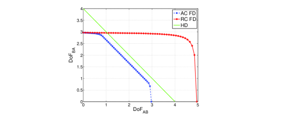
Figure 6: Degrees of Freedom region for two way channel, $N_{A}=4,N_{B}=6,\lambda=0.9$

Figure 6 shows the DoF region for HD, AC FD and RC FD scenarios, where for the FD case we have plotted the convex hull in (9). The corner point of the FD trade-off occurs when SI at one of the nodes is so high (due to high transmission power at that node) that the DoF it receives is effectively zero, even though the other node is transmitting to it. Note that while RC FD can achieve DoF pairs not possible with HD, its DoF region does not contain that of HD.

Next we argue that additional transmit precoding/receive processing to mitigate SI would not improve the FD DoF found above. In order to do this, we will model a two way channel as a full-rank 4-user MIMO interference channel, where transmitting nodes of the interference channel correspond to the transmitting units of the nodes $A$ and $B$, and the receiving nodes correspond to the receiving units. Then, SI cancellation can be viewed as interference cancellation at each receiving node. We further assume $\lambda=0$ and the SI is Gaussian to be able to carry out the signal analysis. Using the MIMO interference channel results in [37] we can show that the maximum sum DoF for the AC scenario with precoding is $\min(N_{A}-1,N_{B}-1)$, obtained with a linear zero forcing precoder. From (9), we see that when $\lambda=0$, substituting $\gamma=0$ (or $\gamma=\infty$) yields the sum DoF of $\min(N_{A}-1,N_{B}-1)$. Since for $\lambda>0$, the sum DoF in (9) would be strictly better, we conclude that transmit precoding does not improve the achievable two way channel DoFs found in this paper. Another advantage of the hardware SI mitigation technique adopted in this paper is that accurate estimates of the SI matrix are not required to implement precoding in the signal space.

IV Two Hop Channel: Relaying

As the second scenario, we consider the two hop channel, where $A$ communicates with $B$ through $R$, as illustrated in Figure 2. Assuming that $B$ does not hear $A$, we formulate, calculate and compare the DoF of two hop communication, i.e., relaying, in HD and FD modes.

IV-A Half-Duplex Mode

In the HD mode, $A$ first transmits to $R$ for a fraction of time, $\tau$, $R$ decodes the received bits and forwards them to $B$ for the remaining fraction, $1-\tau$ of time.

IV-A1 Achievable Rate

The average rate achievable from $A$ to $R$ is calculated as

$$R_{AR}^{HD}=\tau\mathbb{E}\left[\log\det\left(\mathbf{I}+\frac{\Gamma_{AR}}{N_{A}}\mathbf{H}_{AR}\mathbf{H}_{AR}^{*}\right)\right],$$

and the rate achievable over $R$ to $B$ is given by

$$R_{RB}^{HD}=(1-\tau)\mathbb{E}\left[\log\det\left(\mathbf{I}+\frac{\Gamma_{RB}}{N_{R}}\mathbf{H}_{RB}\mathbf{H}_{RB}^{*}\right)\right].$$

By optimizing over $\tau$, the end-to-end average achievable rate for HD relaying can be found as

$$R_{HD}^{AB}=\max_{0\leq\tau\leq 1}\min\left(R_{AR}^{HD},R_{RB}^{HD}\right).$$ (16)

IV-A2 Degrees of Freedom

For the DoF of the two hop channel, as in Section III-B2 we assume that the relay scales its power with respect to the transmission power of node A, according to

$$\frac{\log(P_{R})}{\log(P_{A})}=\gamma,\,\,\,\,0<\gamma\leq 1.$$

Then, the DoF of the relay network in HD mode is given by

$$\text{DoF}_{HD}=\sup_{0<\gamma\leq 1}\lim_{\begin{subarray}{c}P_{A}\to\infty\\ P_{R}=P_{A}^{\gamma}\end{subarray}} \frac{R_{HD}}{\log(P_{A})}$$ (17)

$$=\max_{\begin{subarray}{c}0<\tau<1\\ 0<\gamma\leq 1\end{subarray}}\min( \tau\min(N_{A},N_{R}),$$

$$\gamma(1-\tau)\min(N_{R},N_{B}))$$ (18)

$$=\max_{0<\tau<1}\min (\tau N_{A},\tau N_{R},$$

$$(1-\tau)N_{R},(1-\tau)N_{B}).$$ (19)

Note that, in (18), setting $\gamma=1$ maximizes the $\text{DoF}_{HD}$. Depending on the values of $N_{A}$, $N_{R}$, and $N_{B}$, and using optimal $\tau$ denoted as $\tau_{opt}$, we obtain following DoF values for the HD mode as shown in the Table II.

	$\tau_{opt}$	$\text{DoF}_{HD}$
$N_{R}\leq\min({N_{A},N_{B}})$	$\frac{1}{2}$	$\frac{N_{R}}{2}$
$N_{R}\geq\max({N_{A},N_{B}})$	$\frac{N_{B}}{N_{B}+N_{A}}$	$\frac{N_{A}N_{B}}{N_{B}+N_{A}}$
$N_{A}\leq N_{R}\leq N_{B}$	$\frac{N_{R}}{N_{R}+N_{A}}$	$\frac{N_{R}N_{A}}{N_{R}+N_{A}}$
$N_{B}\leq N_{R}\leq N_{A}$	$\frac{N_{B}}{N_{B}+N_{R}}$	$\frac{N_{R}N_{B}}{N_{R}+N_{B}}$

TABLE II: Degrees of Freedom for HD relaying

IV-B Full-Duplex Mode

In FD relaying, $R$ is able to receive and transmit simultaneously in the same band, however, it is subject to SI. In order to maintain causality, the relay node transmits $(i-1)^{\text{th}}$ symbol, while it receives the $i^{\text{th}}$ symbol.

IV-B1 Achievable Rate

When the relay node operates in FD mode, the rates are calculated as follows:

$$R_{AR}^{FD}=\mathbb{E}\left[\log\det\left(\mathbf{I}+\frac{\Gamma_{AR}}{N_{A}}\mathbf{H}_{AR}\mathbf{H}_{AR}^{\ast}\right)\right],$$

$$R_{RB}^{FD}=\mathbb{E}\left[\log\det\left(\mathbf{I}+\frac{\Gamma_{RB}}{t}\mathbf{H}_{RB}\mathbf{H}_{RB}^{\ast}\right)\right].$$ (20)

Recall that $t=(N_{R}-r)$ for AC FD, and $t=(2N_{R}-2r)$ for RC FD. Depending on the average SINR at the relay node and SNR at $B$, the excess power at the relay can have a negative impact on the achievable rate due to increased SI. In fact, the SINR at the relay node is decreased as the relay power $P_{R}$ is increased, while $P_{A}$ is held constant. Thus, with the increase in $P_{R}$ for a constant $P_{A}$, the rate of the channel from node $A$ to $R$ is decreased, while the rate of the channel from $R$ to node $B$ is increased. Therefore, by letting ${P_{R}}_{max}$ denote the maximum average power at the relay, the achievable rate for FD relaying can be written as

$$R_{FD}^{AD}=\max_{\begin{subarray}{c}0<r<N_{R}\\ P_{R}\leq{P_{R}}_{max}\end{subarray}}\min\left(R_{AR}^{FD},R_{RB}^{FD}\right).$$ (21)

IV-B2 Degrees of Freedom

Assuming power scaling as in (18), the DoF of FD relaying is obtained as

$$\text{DoF}^{FD}_{AB}=\sup_{0<\gamma\leq 1}\lim_{\begin{subarray}{c}{P}_{A}\to\infty\\ {P}_{R}=P_{A}^{\gamma}\end{subarray}}\frac{R_{FD}}{\log(P_{A})},$$

where in order to control the SI, the relay scales its power with respect to the transmission power of node $A$, through

$$\frac{\log(P_{R})}{\log(P_{A})}=\gamma,\,\,\,\,0<\gamma\leq 1.$$

Then, the achievable DoF for FD relaying can be computed as

$$\text{DoF}^{FD}_{AB}=\max_{\begin{subarray}{c}0<r<N_{R}\\ 0<\gamma\leq 1\end{subarray}}\min( (1-\gamma(1-\lambda))\min(N_{A},r),$$

$$\gamma\min(t,N_{B}))$$

$$=\max_{\begin{subarray}{c}0<r<N_{R}\\ 0<\gamma\leq 1\end{subarray}}\min( (1-\gamma(1-\lambda))N_{A},(1-\gamma(1-\lambda))r,$$

$$\gamma t,\gamma N_{B}).$$ (22)

Here, $t=(N_{R}-r)$ for the AC FD implementation and $t=(2N_{R}-2r)$ for the RC FD implementation. We explicitly compute the $\text{DoF}_{AB}^{FD}$ for symmetric and asymmetric cases and compare it with $\text{DoF}_{AB}^{HD}$ in the next subsection.

IV-C Comparison of HD and FD Relaying

• Symmetric Case ($N_{A}=N_{B}$):
  To compare the DoF of HD relaying and FD relaying, we first consider a symmetric case when the $A$ and $B$ have same number of antennas, i.e., $N_{A}$=$N_{B}$=$N$, and $N_{R}$ is even. Using the Table II, one can obtain

  $$\text{DoF}^{HD}_{AB}=\min\left(\frac{N}{2},\frac{N_{R}}{2}\right).$$ (23)

  For AC FD implementation (22) can be written as

  $$\text{DoF}^{FD,AC}_{AB} =\max_{\begin{subarray}{c}1\leq r<N_{R}\\ 0<\gamma\leq 1\end{subarray}}\min((1-\gamma(1-\lambda))N,$$

  $$\qquad\qquad(1-\gamma(1-\lambda))r,(N_{R}-r),\gamma N)$$

  $$\leq\max_{0<\gamma\leq 1}\min((1-\gamma(1-\lambda))N,\gamma N)$$ (24)

  $$=\frac{N}{2-\lambda}.$$ (25)

  Since the minimum of the two terms in (24) is maximized when both are equal, (25) can be obtained by setting $\gamma=\frac{1}{2-\lambda}$. Similarly,

  $$\text{DoF}^{FD,AC}_{AB} \leq\max_{\begin{subarray}{c}1\leq r<N_{R}\\ 0<\gamma\leq 1\end{subarray}}\min((1-\gamma(1-\lambda))r,\gamma(N_{R}-r)),$$

  $$=\frac{N_{R}}{2(2-\lambda)},$$ (26)

  where (26) is obtained by setting $\gamma=\frac{1}{2-\lambda}$ and $r=\frac{N_{R}}{2}$.

  From (25) and (26), we can write

  $$\text{DoF}^{FD,AC}_{AB}\leq\frac{1}{2-\lambda}\min\left(N,\frac{N_{R}}{2}\right).$$ (27)

  Equality in (27) can be achieved when $\gamma=\frac{1}{2-\lambda}$ and $r=\frac{N_{R}}{2}$, leading to

  $$\text{DoF}^{FD,AC}_{AB}=\frac{1}{2-\lambda}\min\left(N,\frac{N_{R}}{2}\right).$$ (28)

  Similarly, for the RC FD implementation we have,

  $$\text{DoF}^{FD,RC}_{AB}=\frac{1}{2-\lambda}\min\left(N,\left\lfloor\frac{2N_{R}}{3}\right\rfloor\right).$$ (29)

  

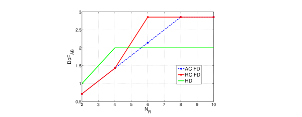
  Figure 7: DoF for HD relaying and FD relaying, $N_{A}$=$N_{B}$=$4$.

  The DoF results for this case are plotted in Figure 7. As seen from the figure, when $N_{R}$ is small, HD relaying performs better than FD relaying, and the situation is reversed when $N_{R}$ gets larger, with the RC FD implementation always dominating AC FD implementation. Comparing (23) and (28), $\text{DoF}^{FD,AC}_{AB}>\text{DoF}^{HD}_{AB}$ if

  $$N_{R}>N(2-\lambda)\quad\text{and}\quad\lambda>0.$$ (30)

  Similarly from (23) and (29), if $N_{R}$ is divisible by $3$, then $\text{DoF}^{FD,RC}_{AB}>\text{DoF}^{HD}_{AB}$ provided

  $$N_{R}>\frac{3}{4}N(2-\lambda)\quad\text{and}\quad\lambda>0.$$ (31)

  If $N_{R}$ is not divisible by $3$, then (23) and (29) can be evaluated to compare $\text{DoF}^{FD,RC}_{AB}$ and $\text{DoF}^{HD}_{AB}$.

• Asymmetric Case ($N_{A}=1$):
  Now, we consider the asymmetric case, where node $A$ has a single antenna, i.e., $N_{A}=1$, whereas the relay and node $B$ have multiple antennas, $N_{R}$ and $N_{B}\geq 1$, respectively. This could model a cellular phone, which cannot afford multiple antennas, communicating with an access point through a relay.

  From the general expression for the DoF for the FD relaying channel for both AC and RC implementation, (22) with $N_{A}=1$

  $$\text{DoF}^{FD}_{AB} =\max_{\begin{subarray}{c}0<r<N_{R}\\ 0<\gamma\leq 1\end{subarray}}\min((1-\gamma(1-\lambda)),(1-\gamma(1-\lambda))r,$$

  $$\quad\qquad\qquad\qquad\gamma(N_{R}-r),\gamma N_{B})$$ (32)

  $$=\max_{0<\gamma\leq 1}\min((1-\gamma(1-\lambda)),\gamma(N_{R}-1),\gamma N_{B})$$ (33)

  $$=\frac{\min(N_{R}-1,N_{B})}{\min(N_{R}-1,N_{B})+1-\lambda}$$ (34)

  where we have set $r=1$ in (33) since the minimum of first two terms in (32) does not depend on $r$ and the third term is decreasing in $r$.

  The DoF for HD relaying yields

  $$\text{DoF}^{HD}_{AB}=\frac{\min(N_{R},N_{B})}{\min(N_{R},N_{B})+1},$$

  It can be seen that $\text{DoF}^{FD}_{AB}>\text{DoF}^{HD}_{AB}$ if

  $$\lambda>1-\frac{\min(N_{R}-1,N_{B})}{\min(N_{R},N_{B})}.$$

  Hence, for both AC FD and RC FD implementations, the following holds: If $N_{R}>N_{B}$, then DoF of FD relaying is strictly larger than DoF of HD relaying for both AC FD and RC FD implementations, provided $\lambda>0$. If $N_{R}\leq N_{B}$, then FD relaying performs better than HD relaying if $\lambda>\frac{1}{N_{R}}$. Thus the FD implementation is better than the HD if

  $$N_{R}>\min\left(N_{B},\frac{1}{\lambda}\right).$$ (35)

It is interesting to note that, for the case $N_{A}=N_{B}=1$, and $N_{R}=2$, [13] obtained the DoF (referred to as multiplexing gain in [13]) for FD relaying channel, with the relay node operating in amplify and forward mode, using a similar SI model as in this paper. Their multiplexing gain term of $\frac{1}{2-\lambda}$ matches with our DoF, when evaluated at $N=1$, and $N_{R}=2$ in (28).

V Two Way Two Hop Channel: Two Way Relaying

As the third scenario, we consider the two way two hop channel, where $A$ and $B$ communicate with each other through $R$, performing two way relaying, as illustrated in Figures 3 and 4 representing HD and FD modes, respectively. Again, there is no direct link between nodes $A$ and $B$. We formulate, calculate and compare the achievable rates as well as DoF of two way two hop communication in HD and FD modes.

V-A Half-Duplex Mode

V-A1 Achievable Rates

In HD mode, with transmission strategies described in the corresponding system model in Section II-B , the average achievable rates can be calculated as follows: During the MAC phase, both nodes $A$ and $B$ transmit their messages to the relay node with achievable rates calculated as [16],

$$R^{HD}_{AR}\leq\tau\mathbb{E}\left[\log\det\left(\mathbf{I}+\frac{{\Gamma}_{AR}}{N_{A}}\mathcal{H}_{AR}\mathbf{H}_{AR}^{\ast}\right)\right],$$

$$R^{HD}_{BR}\leq\tau\mathbb{E}\left[\log\det\left(\mathbf{I}+\frac{\Gamma_{BR}}{N_{B}}\mathbf{H}_{BR}\mathbf{H}_{BR}^{\ast}\right)\right],$$

$$R^{HD}_{AR}+R^{HD}_{BR}\leq\tau\mathbb{E}\left[\log\det\left(\mathbf{I}+\frac{{\Gamma}_{AR}}{N_{A}}\mathbf{H}_{AR}\mathbf{H}_{AR}^{\ast}\right.\right.$$

$$\qquad\qquad\qquad\qquad+\left.\left.\frac{\Gamma_{BR}}{N_{B}}\mathbf{H}_{BR}\mathbf{H}_{BR}^{\ast}\right)\right].$$

Here we assume that MAC phase lasts for $\tau$ fraction of the time. During the BC phase, the relay node broadcasts a message to both of the nodes, such that each node can retrieve the other node’s message by subtracting its own data. The achievable rates for this phase are obtained as [16],

$$R^{HD}_{RA}\leq\left(1-\tau\right)\mathbb{E}\left[\log\det\left(\mathbf{I}+\frac{{\Gamma}_{RA}}{N_{R}}\mathbf{H}_{RA}\mathbf{H}_{RA}^{\ast}\right)\right],$$

$$R^{HD}_{RB}\leq\left(1-\tau\right)\mathbb{E}\left[\log\det\left(\mathbf{I}+\frac{{\Gamma}_{RB}}{N_{R}}\mathbf{H}_{RB}\mathbf{H}_{RB}^{\ast}\right)\right].$$

Then, the end-to-end rates are obtained as

$$R^{HD}_{AB}=\min\left(R_{AR},R_{RB}\right),R^{HD}_{BA}=\min\left(R_{BR},R_{RA}\right).$$

The BC phase is assumed to last $(1-\tau)$ fraction of the time.

Note that, dropping the sum rate constraint from the MAC phase gives the cut-set upper bound for the HD two way two hop channel [38].

V-A2 Degrees of Freedom

We compute an upper bound for DoF for HD two way two hop channel, which we later compare with the performance of FD two way two hop channel. We also compare FD with the achievable MAC-BC HD scheme introduced above.

During the first phase, which is assumed to be used for the fraction $\tau$ of time, the $\text{DoF}_{{AR}}$ and $\text{DoF}_{{BR}}$ are upper bounded by the respective point-to-point DoFs, i.e.,

$$\text{DoF}_{{AR}}\leq\tau\min(N_{A},N_{R}),\,\text{DoF}_{{BR}}\leq\tau\min(N_{B},N_{R}).$$

Similarly, during the second phase, the DoF expressions are

$$\text{DoF}_{RA}\leq(1-\tau)\min(N_{A},N_{R}),$$

$$\text{DoF}_{{RB}}\leq(1-\tau)\min(N_{B},N_{R}).$$

The achievable DoF with MAC-BC scheme has an additional sum constraint

$$\text{DoF}_{RA}+\text{DoF}_{{RB}}\leq(1-\tau)\min(2N_{A},N_{R}).$$

Hence, the upper bound on end-to-end DoF is

$$\text{DoF}_{{AB}} \leq\min(\text{DoF}_{{AR}},\text{DoF}_{{RB}})$$

$$=\min(\tau N_{A},\tau N_{R},(1-\tau)N_{R},(1-\tau)N_{B}),$$

$$\text{DoF}_{{BA}} \leq\min(\text{DoF}_{{BR}},\text{DoF}_{{RA}})$$

$$=\min(\tau N_{B},\tau N_{R},(1-\tau)N_{R},(1-\tau)N_{A}).$$

For the symmetric case $N_{A}=N_{B}=N$, $\tau=\frac{1}{2}$ maximally enlarges the outer bound region, i.e.,

$$\mathtt{DoF}^{HD}_{UB}=\bigg{\{} \text{DoF}_{{AB}},\text{DoF}_{{BA}}\in\mathbb{R}^{2}:$$

$$\text{DoF}_{{AB}}\leq\min\left(\frac{N}{2},\frac{N_{R}}{2}\right)$$

$$\text{DoF}_{{BA}}\leq\min\left(\frac{N}{2},\frac{N_{R}}{2}\right)\bigg{\}}.$$

Similarly, taking $\tau=\frac{1}{2}$ gives the following achievable DoF region with MAC-BC scheme

$$\mathtt{DoF}^{HD}_{DF}=\bigg{\{} \left(\text{DoF}_{{AB}},\text{DoF}_{{BA}}\right)\in\mathbb{R}^{2}:$$

$$\text{DoF}_{{AB}}\leq\min\left(\frac{N}{2},\frac{N_{R}}{2}\right)$$

$$\text{DoF}_{{BA}}\leq\min\left(\frac{N}{2},\frac{N_{R}}{2}\right)$$

$$\text{DoF}_{{AB}}+\text{DoF}_{{BA}}\leq\min\left(N,\frac{N_{R}}{2}\right)\bigg{\}}.$$ (36)

V-B Full-Duplex Mode

In this section, we assume only $R$ is FD enabled, and $A$ and $B$ are HD nodes. As described in the corresponding system model in Section II-B, FD two way two hop communication takes place in two phases assigned for each direction, where $A$ and $B$ send data to each other, as $R$ performs FD relaying. Again, it is assumed that the fraction of time devoted to first phase is denoted by $\tau$, and the remaining fraction, $1-\tau$, is assigned to the second phase.

V-B1 Achievable Rates

According to SINR expressions at the nodes, the average rates are calculated through the following expressions:

$$R^{FD}_{AR} \leq\mathbb{E}\left[\log\det\left({\mathbf{I}}+\frac{{\Gamma}_{AR}}{N_{A}}\mathbf{H}_{AR}\mathbf{H}_{AR}^{\ast}\right)\right],$$

$$R^{FD}_{RB} \leq\mathbb{E}\left[\log\det\left({\mathbf{I}}+\frac{{\Gamma}_{RB}}{t}\mathbf{H}_{RB}\mathbf{H}_{RB}^{\ast}\right)\right],$$

$$R^{FD}_{BR} \leq\mathbb{E}\left[\log\det\left({\mathbf{I}}+\frac{{\Gamma}_{BR}}{N_{B}}\mathbf{H}_{BR}\mathbf{H}_{BR}^{\ast}\right)\right],$$

$$R^{FD}_{RA} \leq\mathbb{E}\left[\log\det\left({\mathbf{I}}+\frac{{\Gamma}_{RA}}{t}\mathbf{H}_{RA}\mathbf{H}_{RA}^{\ast}\right)\right].$$

The end-to-end average rate is given by the following expressions,

$$R^{FD}_{AB}=\tau\min\left(R_{AR},R_{RB}\right),R^{FD}_{BA}=(1-\tau)\min\left(R_{BR},R_{RA}\right).$$

V-B2 Degrees of Freedom

Since only $R$ is FD capable, the DoF achievable from node $A$ to node $B$ is given as in Section IV-B. Letting $D^{FD}_{AB}$ and $D^{FD}_{BA}$ be DoFs obtained when communication takes place from the node $A$ to the node $B$, and in the reverse direction respectively, the DoF trade off region is obtained via time sharing as follows:

$${\mathtt{DoF}}^{FD}=\left\{\right. (\text{DoF}^{FD}_{{AB}},\text{DoF}_{{BA}}^{FD})\in\mathbb{R}^{2}:$$

$$\text{DoF}_{{AB}}\leq\tau D_{AB}^{FD},\text{DoF}_{{BA}}\leq(1-\tau)D_{BA}^{FD}$$

$$\left.0\leq\tau\leq 1\right\}.$$

Here, $D_{AB}^{FD}$ is given by (22),

$$D^{FD}_{AB}=\max_{\begin{subarray}{c}0<r<N_{R}\\ 0<\gamma\leq 1\end{subarray}}\min( (1-\gamma(1-\lambda))N_{A},(1-\gamma(1-\lambda))r,$$

$$\gamma t,\gamma N_{B}).$$

A similar expression holds for $D_{BA}^{FD}$. We explicitly evaluate and compare the DoF regions of HD and FD two way relaying for some specific cases in the next subsection.

V-C Comparison of HD and FD Two Way Relaying

Again, we consider the symmetric and asymmetric scenarios as follows.

• Symmetric Case ($N_{A}=N_{B}$):
  If the nodes $A$ and $B$ have same number of antennas ($N_{A}=N_{B}=N$), and $N_{R}$ is even then the DoF region for the AC FD implementation is obtained as from Section IV-C

  $${\mathtt{DoF}}^{FD}=\bigg{\{} (\text{DoF}_{{AB}},\text{DoF}_{{BA}})\in\mathbb{R}^{2}:$$

  $$\text{DoF}_{{AB}}\leq\frac{\tau}{2-\lambda}\min\left(\frac{N_{R}}{2},N\right)$$

  $$\text{DoF}_{{BA}}\leq\frac{1-\tau}{2-\lambda}\min\left(\frac{N_{R}}{2},N\right)$$

  $$0\leq\tau\leq 1\bigg{\}}.$$

  Note that, the corner point of this trade-off is $\left(\frac{1}{2-\lambda}\min\left(\frac{N_{R}}{2},N\right),0\right)$, which is better than the corner point of for the HD case $\left(\min\left(\frac{N_{R}}{2},\frac{N}{2}\right),0\right)$ provided

  $$N_{R}>(2-\lambda)N\,\text{and}\,\lambda>0.$$

  Hence, if $R$ has sufficient number of antennas, then some part of the FD DoF region lies outside the HD DoF upper bound.

  Similarly, for the RC FD implementation, the DoF region is given by

  $${\mathtt{DoF}}^{FD}=\bigg{\{} (\text{DoF}_{{AB}},\text{DoF}_{{BA}})\in\mathbb{R}^{2}:$$

  $$\text{DoF}_{{AB}}\leq\frac{\tau}{2-\lambda}\min\left(\left\lfloor\frac{2N_{R}}{3}\right\rfloor,N\right)$$

  $$\text{DoF}_{{BA}}\leq\frac{1-\tau}{2-\lambda}\min\left(\left\lfloor\frac{2N_{R}}{3}\right\rfloor,N\right)$$

  $$0\leq\tau\leq 1\bigg{\}}.$$ (37)

  Hence the condition for some part of the FD DoF region for RC FD implementation to lie outside the upper bound of HD one is (provided $N_{R}$ is divisible by $3$; see (31))

  $$N_{R}>\frac{3(2-\lambda)}{4}N\,\text{and}\,\lambda>0.$$ (38)

  An example comparing the DoF trade off for the symmetric case can be seen in Figure 8, where we have plotted the upper bound for the HD trade-off, an achievable HD trade-off through MAC-BC scheme, and the FD AC and RC trade-off. It can be observed that near the corner points, where one of the node’s DoF is small, the AC trade-off is better than the HD trade-off. However near the central region when both of the node’s DoF is nearly equal HD trade-off is better.

  

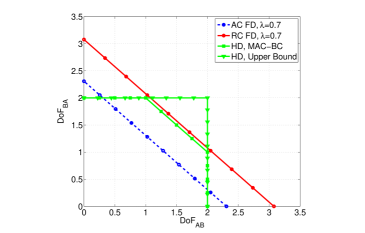
  Figure 8: DoF trade-off for HD and FD two way relaying, $N_{A}=N_{B}=N=4$, $N_{R}=6$.

• Asymmetric Case ($N_{A}=1$):
  Using the time sharing and expressions obtained for DoF for the asymmetric case in Section IV-C, the DoF region for FD (both AC and RC) can be written as,

  $${\mathtt{DoF}}^{FD}=\Big{\{} (\text{DoF}_{{AB}},\text{DoF}_{{BA}})\in\mathbb{R}^{2}:$$

  $$\text{DoF}_{{AB}}\leq\frac{\tau\min(N_{R}-1,N_{B})}{\min(N_{R}-1,N_{B})+1-\lambda}$$

  $$\text{DoF}_{{BA}}\leq\frac{(1-\tau)\min(N_{R}-1,N_{B})}{\min(N_{R}-1,N_{B})+1-\lambda}$$

  $$0\leq\tau\leq 1\Big{\}}.$$

  Comparing with the DoF upper bound for HD, we conclude that some part of the FD DoF region lies outside the HD one provided (see (35))

  $$N_{R}>\min\left(N_{B},\frac{1}{\lambda}\right).$$

VI Conclusions

In this paper, we have compared DoF for three communication scenarios: two way, two hop, and two way two hop. Using the antenna conserved and RF chain conserved implementations of FD with a realistic residual SI model, we have investigated the conditions under which FD can provide higher throughput than HD. Through detailed DoF analysis, for the two way channel, we have found that the achievable DoF for AC FD is not better than HD with imperfect SI cancellation. For the RC FD case, however, FD DoF trade-off can be better, when the SI cancellation parameter $\lambda$ is high enough. The cross over point depends on various system parameters. In case of the two hop channel, FD is better when the relay has sufficient number of antennas and $\lambda$ is high enough. For the two way two hop channel, when both of nodes require similar throughput, the HD implementation is generally better than FD. However, when one of the terminal’s data rate requirement is significantly higher than the other’s (e.g., when data flow occurs mostly in one direction, and the other direction is only used for feedback and control information, or in the case of asymmetric uplink and downlink data rates), then FD can achieve better DoF pairs than HD, provided the relay has sufficient number of antennas and the SI suppression factor $\lambda$ is high enough.

It should be mentioned that although the DoF results presented for FD are achievable, and the converse results appear to be difficult to obtain, we believe that sophisticated techniques such as zero-forcing, beamforming, or receive processing cannot improve this DoF. Hence the cases for which HD performs better than the achievable FD considered here should still hold true.

The presented results in this paper provide guidelines for choosing HD or FD implementation in practical systems. Future research directions include studying more complex communication scenarios with inter-node interference and different relaying protocols, where the model and techniques used in this paper may provide a useful foundation.

References

- [1] N. Shende, O. Gurbuz, and E. Erkip, “Half-duplex or full-duplex relaying: A capacity analysis under self-interference,” in 47th Annual Conference on Information Sciences and Systems, March 2013, pp. 1–6.
- [2] M. Duarte and A. Sabharwal, “Full-duplex wireless communications using off-the-shelf radios: Feasibility and first results,” in Forty Fourth Asilomar Conference on Signals, Systems and Computers, Nov. 2010, pp. 1558 –1562.
- [3] M. Knox, “Single antenna full duplex communications using a common carrier,” in 13th Annual Wireless and Microwave Technology Conference, Apr 2012.
- [4] J. I. Choi, M. Jain, K. Srinivasan, P. Levis, and S. Katti, “Achieving single channel, full duplex wireless communication,” in Proceedings of the Sixteenth Annual International Conference on Mobile Computing and Networking, 2010, pp. 1–12.
- [5] M. A. Khojastepour, K. Sundaresan, S. Rangarajan, X. Zhang, and S. Barghi, “The case for antenna cancellation for scalable full-duplex wireless communications,” in Proceedings of the 10th ACM Workshop on Hot Topics in Networks, 2011, pp. 17:1–17:6.
- [6] M. Jain, J. I. Choi, T. Kim, D. Bharadia, S. Seth, K. Srinivasan, P. Levis, S. Katti, and P. Sinha, “Practical, real-time, full duplex wireless,” in 17th Annual International Conference on Mobile Computing and Networking, Sept. 2011, pp. 301–312.
- [7] A. Sabharwal, P. Schniter, D. Guo, D. Bliss, S. Rangarajan, and R. Wichman, “In-band full-duplex wireless: Challenges and opportunities,” IEEE Journal on Selected Areas in Communications, vol. 32, no. 9, pp. 1637–1652, Sept 2014.
- [8] D. Bharadia, E. McMilin, and S. Katti, “Full duplex radios,” SIGCOMM Comput. Commun. Rev., vol. 43, no. 4, pp. 375–386, Aug. 2013.
- [9] B. Day, A. Margetts, D. Bliss, and P. Schniter, “Full-duplex MIMO relaying: Achievable rates under limited dynamic range,” IEEE Journal on Selected Areas in Communications, vol. 30, no. 8, pp. 1541 –1553, Sept. 2012.
- [10] T. Riihonen, S. Werner, and R. Wichman, “Hybrid full-duplex/half-duplex relaying with transmit power adaptation,” IEEE Transactions on Wireless Communications, vol. 10, no. 9, pp. 3074–3085, Sept 2011.
- [11] D. Ng, E. Lo, and R. Schober, “Dynamic resource allocation in MIMO-OFDMA systems with full-duplex and hybrid relaying,” IEEE Transactions on Communications, vol. 60, no. 5, pp. 1291–1304, May 2012.
- [12] M. Duarte, C. Dick, and A. Sabharwal, “Experiment-driven characterization of full-duplex wireless systems,” IEEE Transactions on Wireless Communications, vol. 11, no. 12, pp. 4296–4307, December 2012.
- [13] L. Jimenez Rodriguez, N. Tran, and T. Le-Ngoc, “Optimal power allocation and capacity of full-duplex af relaying under residual self-interference,” IEEE Wireless Communications Letters, vol. 3, no. 2, pp. 233–236, April 2014.
- [14] S. Barghi, A. Khojastepour, K. Sundaresan, and S. Rangarajan, “Characterizing the throughput gain of single cell mimo wireless systems with full duplex radios,” in 10th International Symposium on Modeling and Optimization in Mobile, Ad Hoc and Wireless Networks, May 2012, pp. 68–74.
- [15] V. Aggarwal, M. Duarte, A. Sabharwal, and N. K. Shankaranarayanan, “Full- or half-duplex? A capacity analysis with bounded radio resources,” in IEEE Information Theory Workshop, Sep 2012.
- [16] D. Tse and P. Viswanath, Fundamentals of Wireless Communication. New York, NY, USA: Cambridge University Press, 2005.
- [17] H. Ju, X. Shang, H. Poor, and D. Hong, “Bi-directional use of spatial resources and effects of spatial correlation,” IEEE Transactions on Wireless Communications, vol. 10, no. 10, pp. 3368–3379, October 2011.
- [18] D. Kim, H. Ju, S. Park, and D. Hong, “Effects of channel estimation error on full-duplex two-way networks,” IEEE Transactions on Vehicular Technology, vol. 62, no. 9, pp. 4666–4672, Nov 2013.
- [19] A. Arifin and T. Ohtsuki, “Outage probability analysis in bidirectional full-duplex siso system with self-interference,” in Asia-Pacific Conference on Communications, Oct 2014, pp. 6–8.
- [20] K. Akcapinar and O. Gurbuz, “Full-duplex bidirectional communication under self-interference,” in 13th International Conference on Telecommunications, July 2015, pp. 1–7.
- [21] D. Bharadia and S. Katti, “Full duplex mimo radios,” in Proceedings of the 11th USENIX Conference on Networked Systems Design and Implementation, 2014, pp. 359–372.
- [22] M. Pashazadeh and F. Tabataba, “Performance analysis of one-way relay networks with channel estimation errors and loop-back interference,” in 23rd Iranian Conference on Electrical Engineering, May 2015, pp. 432–437.
- [23] S. Goyal, P. Liu, S. Panwar, R. Difazio, R. Yang, J. Li, and E. Bala, “Improving small cell capacity with common-carrier full duplex radios,” in IEEE International Conference on Communications, June 2014, pp. 4987–4993.
- [24] H. Alves, D. Benevides da Costa, R. Demo Souza, and M. Latva-aho, “On the performance of two-way half-duplex and one-way full-duplex relaying,” in IEEE 14th Workshop on Signal Processing Advances in Wireless Communications, June 2013, pp. 56–60.
- [25] G. Liu, F. Yu, H. Ji, V. Leung, and X. Li, “In-band full-duplex relaying: A survey, research issues and challenges,” IEEE Communications Surveys & Tutorials, vol. 17, no. 2, pp. 500–524, Secondquarter 2015.
- [26] A. Goldsmith, Wireless Communications. New York, NY, USA: Cambridge University Press, 2005.
- [27] S. Diggavi and T. Cover, “The worst additive noise under a covariance constraint,” IEEE Transactions on Information Theory, vol. 47, no. 7, pp. 3072–3081, Nov 2001.
- [28] I. Shomorony and A. Avestimehr, “Worst-case additive noise in wireless networks,” IEEE Transactions on Information Theory, vol. 59, no. 6, pp. 3833–3847, June 2013.
- [29] C. E. Shannon, “Two-way communication channels,” in Proceedings of the Fourth Berkeley Symposium on Mathematical Statistics and Probability, Volume 1: Contributions to the Theory of Statistics, 1961, pp. 611–644.
- [30] C. Esli and A. Wittneben, “One- and two-way decode-and-forward relaying for wireless multiuser MIMO networks,” in IEEE Global Telecommunications Conference, Nov 2008, pp. 1–6.
- [31] T. Oechtering, C. Schnurr, I. Bjelakovic, and H. Boche, “Broadcast capacity region of two-phase bidirectional relaying,” IEEE Transactions on Information Theory, vol. 54, no. 1, pp. 454–458, 2008.
- [32] S. Katti, S. Gollakota, and D. Katabi, “Embracing wireless interference: Analog network coding,” SIGCOMM Comput. Commun. Rev., vol. 37, no. 4, pp. 397–408, Aug. 2007.
- [33] S. Zhang, S. C. Liew, and P. P. Lam, “Hot topic: Physical-layer network coding,” in Proceedings of the 12th Annual International Conference on Mobile Computing and Networking, 2006, pp. 358–365.
- [34] J. I. Choi, S. Hong, M. Jain, S. Katti, P. Levis, and J. Mehlman, “Beyond full duplex wireless,” in Forty Sixth Asilomar Conference on Signals, Systems and Computers, Nov 2012, pp. 40–44.
- [35] E. Everett, C. Shepard, L. Zhong, and A. Sabharwal, “Softnull: Many-antenna full-duplex wireless via digital beamforming,” IEEE Transactions on Wireless Communications, vol. 15, no. 12, pp. 8077–8092, Dec 2016.
- [36] A. Shojaeifard, K. Wong, M. D. Renzo, G. Zheng, K. A. Hamdi, and J. Tang, “Self-interference in full-duplex multi-user MIMO channels,” CoRR, vol. abs/1701.00277, 2017.
- [37] S. A. Jafar and M. J. Fakhereddin, “Degrees of freedom for the MIMO interference channel,” IEEE Transactions on Information Theory, vol. 53, no. 7, pp. 2637–2642, July 2007.
- [38] R. Knopp, “Two-way wireless communication via a relay station,” in GDR-ISIS meeting, Mar. 2007.