First detection of gas-phase ammonia in a planet-forming disk

Abstract

Context. Nitrogen chemistry in protoplanetary disks and the freeze-out on dust particles is key to understand the formation of nitrogen bearing species in early solar system analogs. In dense cores, 10% to 20% of the nitrogen reservoir is locked up in ices like NH₃, NH${}_{4}^{+}$ and OCN^-. So far, ammonia has not been detected beyond the snowline in protoplanetary disks.

Aims. We aim to find gas-phase ammonia in a protoplanetary disk and characterize its abundance with respect to water vapor.

Methods. Using HIFI on the Herschel Space Observatory we detect, for the first time, the ground-state rotational emission of ortho-NH₃ in a protoplanetary disk, around TW Hya. We use detailed models of the disk’s physical structure and the chemistry of ammonia and water to infer the amounts of gas-phase molecules of these species. We explore two radial distributions (extended across the disk and confined to $<$60 au like the millimeter-sized grains) and two vertical distributions (near the midplane and at intermediate heights above the midplane, where water is expected to photodesorb off icy grains) to describe the (unknown) location of the molecules. These distributions capture the effects of radial drift and vertical settling of ice-covered grains.

Results. The NH₃ $1_{0}$–$0_{0}$ line is detected simultaneously with H₂O $1_{10}$–$1_{01}$ at an antenna temperature of 15.3 mK in the Herschel beam; the same spectrum also contains the N₂H⁺ 6–5 line with a strength of 18.1 mK. We use physical-chemical models to reproduce the fluxes with assuming that water and ammonia are co-spatial. We infer ammonia gas-phase masses of 0.7-11.0 $\times$10²¹ g, depending on the adopted spatial distribution, in line with previous literature estimates. For water, we infer gas-phase masses of 0.2-16.0 $\times$10²² g, improving upon earlier literature estimates This corresponds to NH₃/H₂O abundance ratios of 7%-84%, assuming that water and ammonia are co-located. The inferred N₂H⁺ gas mass of 4.9$\times 10^{21}$ g agrees well with earlier literature estimates based on lower excitation transitions. This masses correspond to a disk-averaged abundances of 0.2–17.0$\times 10^{-11}$, 0.1–9.0$\times 10^{-10}$ and 7.6$\times 10^{-11}$ for NH₃, H₂O and N₂H⁺ respectively.

Conclusions. Only in the most compact and settled adopted configuration is the inferred NH₃/H₂O consistent with interstellar ices and solar system bodies of $\sim$ 5%–10%; all other spatial distributions require addition gas-phase NH₃ production mechanisms. Volatile release in the midplane may occur via collisions between icy bodies if the available surface for subsequent freeze-out is significantly reduced, e.g., through growth of small grains into pebbles or larger.

1 Introduction

The main reservoir of nitrogen-bearing species in most solar-system bodies is unknown. The dominant form of nitrogen on these bodies is inherited from the chemical composition of the solar nebula when planetesimals were formed (Schwarz & Bergin, 2014; Mumma & Charnley, 2011). This composition depends strongly on the initial abundances, which are difficult to probe since N and $\rm{N_{2}}$ are not directly observable in the interstellar medium (ISM). The Spitzer ‘Cores to Disks’ program found that on average 10% to 20% of nitrogen is contained in ices like $\rm{NH_{3}}$, $\rm{NH_{4}^{+}}$, and $\rm{XCN}$, mostly in the form of OCN^- (Öberg et al., 2011a). Water is the most abundant volatile in interstellar ices and cometary ices. The relative abundance of the main nitrogen-bearing species compared to water are of the order of a few percent; $\sim$ 5% for ammonia and $\sim$ 0.3% for $\rm{XCN}$ (Bottinelli et al., 2010; Öberg et al., 2011a). CN and HCN have been detected in later stages of star formation toward protoplanetary disks (see Dutrey et al., 1997; Thi et al., 2004; Öberg et al., 2011b; Guilloteau et al., 2013) along with resolved N₂H⁺ emission in TW Hya (Qi et al., 2013) and unresolved N₂H⁺ emission in several other disks (Dutrey et al., 2007; Öberg et al., 2010, 2011b). Although some upper limits exist for NH₃ in protoplanetary disks in the near-infrared (Salyk et al., 2011; Mandell et al., 2012), there are no published detections at the moment.

Here we report the first detection of NH₃ along with the N₂H⁺ 6–5 line in the planet-forming disk around TW Hya using the HIFI instrument on the Herschel Space Observatory. This disk has already been well studied. It was first imaged by the Hubble Space Telescope (HST) (Krist et al., 2000; Weinberger et al., 2002) revealing a nearly face-on orientation. Roberge et al. (2005) took new HST images confirming this orientation and measured scattered light up to 280 au. Submillimeter interferometric CO data suggest an inclination of $6^{\circ}$ to $7^{\circ}$ (Qi et al., 2004; Rosenfeld et al., 2012). The age of TW Hya is estimated to be 8–10 Myr (Hoff et al., 1998; Webb et al., 1999; de la Reza et al., 2006; Debes et al., 2013) at a distance of 54 $\pm$ 6 pc (Rucinski & Krautter, 1983; Wichmann et al., 1998; van Leeuwen, 2007).

This paper attempts to model the ammonia emission coming from TW Hya assuming that it is desorbed simultaneously with water. The thermal desorption characteristics of ammonia are similar to those of water (Collings et al., 2004). The non-thermal desorption of ammonia via photodesorption has a similiar rate to that of water, within a factor of three (Öberg, 2009). Ammonia is frozen in water-rich ice layers present on interstellar dust particles. Therefore, we can expect both molecules to be absent from the gas phase within similar regions. In order to properly constrain the NH₃/H₂O ratio we need to revisit past models of water emission in the disk surrounding TW Hya.

The ground-state rotational emission for both of the water spin isomers has been found around TW Hya by Hogerheijde et al. (2011) (from now on H11), also using the HIFI instrument on Herschel Space Observatory. They explained this emission using the physical model from Thi et al. (2010) to calculate the amount of water that can be produced by photodesorption from a hidden reservoir of water in the form of ice on dust grains (Bergin et al., 2010; van Dishoeck et al., 2014). Their model overestimates the total line flux by a factor of 3–5. They explore different ways to reduce the amount of water flux and conclude that settling of large icy grains is the only viable way to fit the data.

Here, we re-derive estimates of the amount of water vapor, using an updated estimate of the disk gas mass and considering the effect of a more compact distribution of millimeter-size grains, due to radial drift, as well as settling. These dust processes are relevant for the molecular abundance of water because they can potentially move the bulk of the ice reservoir away from regions where photodesorption is effective. Simultaneously, we estimate the amount of NH₃ using the detection of ammonia in the Herschel spectra, and derive constraints on the NH₃/H₂O ratio in the disk gas, assuming that NH₃ and H₂O are co-spatial. We also estimate the amount of N₂H⁺ and compare it to the amount of NH₃ using a simple parametric model. Section 2 presents our data and their reduction. Section 3 contains our modeling approach and Section 4 the resulting ammonia and water vapor masses. Section 5 discusses the validity of our models and compares these predictions to standard values. Finally section 6 summarizes our conclusions.

2 Observations

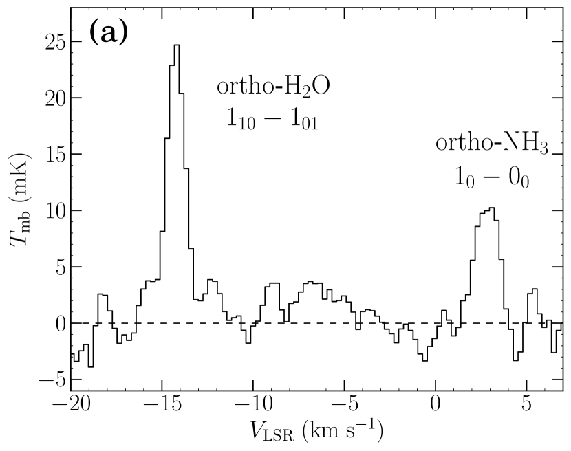
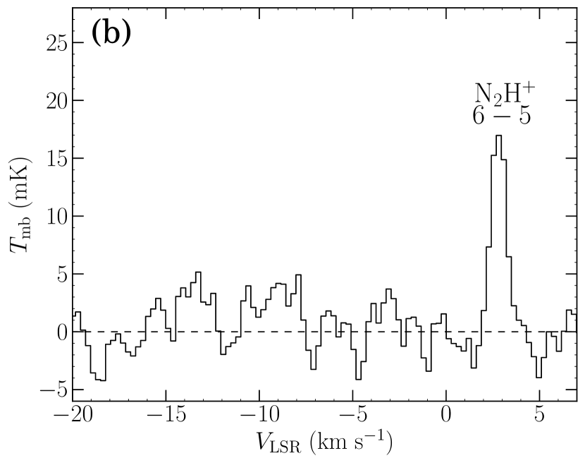
Figure 1: Observed spectra of (a) ortho-NH₃ $1_{0}-0_{0}$, ortho-H₂O $1_{10}-1_{01}$ (earlier presented by H11), and (b) N₂H⁺ 6–5, using Herschel WBS. The dashed line shows the continuum-subtracted spectral baseline. The o-H₂O and o-NH₃ lines are observed in opposite sidebands, causing the o-H₂O to show up at a velocity of $-$14 km s^-1 in panel (a).

Observations of TW Hya ($\rm\alpha_{2000}$ = ${\rm 11^{h}01^{m}51{\aas@@fstack{s}}91}$, $\delta_{2000}$ = $-34^{\circ}42^{\prime}17{\aas@@fstack{\prime\prime}}0$) were previously presented by H11 and obtained using the Heterodyne Instrument for the Far-Infrared (HIFI) as part of the ‘Water in Star-Forming Regions with Herschel’ (WISH) key program (van Dishoeck et al., 2011). We now present observations taken on 2010 June 15 of the NH₃ $1_{0}-0_{0}$ line at 572.49817 GHz simultaneously with o-H₂O at 556.93607 GHz using receiver band 1b and a local oscillator tuning of 551.895 GHz (OBS-ID 1342198337). We also present the detection of N₂H⁺ 6–5 at 558.96651 GHz in the same spectrum. With a total on-source integration of 326 min, the observation was taken with system temperatures of $360$–$400$ K. The data were recorded in the Wide-Band Spectrometer (WBS) which covers 4.4 GHz with 1.1 MHz resolution. This corresponds to 0.59 km s^-1 at 572 GHz. The data were also recorded in the High-Resolution Spectrometer (HRS) which covers 230 MHz at a resolution of 0.25 MHz resulting in 0.13 km s^-1 at the observed frequency of the NH₃ $1_{0}-0_{0}$ line. The calibration procedure is identical to the one of H11, but employs an updated beam efficiency of $\eta_{\rm{mb}}=0.635$ and a HPBW of $36{\aas@@fstack{\prime\prime}}1$ increasing the reported water line fluxes by about 17% with respect to the values of H11. Table 1 summarizes the line fluxes of ammonia, water and N₂H⁺ 6–5. Figure 1 shows the calibrated spectra of ortho-ammonia, ortho-water and N₂H⁺ 6–5 lines.

Table 1: Observed line parameters.

Transition	$F_{\rm{line}}$ $\rm{(10^{-19}\leavevmode\nobreak\ Wm^{-2})}$	$V_{\rm LSR}$ (${\rm km\,s^{-1}}$)	FWHM (${\rm km\,s^{-1}}$)	$\rm{T_{mb}}$ $(\rm{mK})$
NH3 $1_{0}-0_{0}$ (HRS)	1.1$\pm$0.13	3.0$\pm$0.06	0.9$\pm$0.06	15.3$\pm$3.6
NH3 $1_{0}-0_{0}$ (WBS)	1.1$\pm$0.10	2.9$\pm$0.06	1.4$\pm$0.06	11.3$\pm$2.0
N2H+ 6–5 (WBS)	1.0$\pm$0.11	2.9$\pm$0.03	0.9$\pm$0.04	18.1$\pm$2.4
o-H2O $1_{10}-1_{01}$ (HRS)	1.8$\pm$0.11	2.8$\pm$0.02	0.9$\pm$0.02	30.7$\pm$3.7
o-H2O $1_{10}-1_{01}$ (WBS)	1.9$\pm$0.09	2.9$\pm$0.03	1.3$\pm$0.03	24.0$\pm$2.0
p-H2O $1_{11}-0_{00}$ (HRS)	6.7$\pm$0.62	2.7$\pm$0.05	1.1$\pm$0.05	41.0$\pm$8.1
p-H2O $1_{11}-0_{00}$ (WBS)	6.7$\pm$0.44	2.7$\pm$0.04	1.3$\pm$0.04	39.0$\pm$5.2

3 Modeling approach

Since NH₃ is intermixed with H₂O on interstellar ices and it is thought to desorb simultaneously (Öberg, 2009), our modeling approach focuses on deriving a NH₃/H₂O ratio in the TW Hya disk assuming that the NH₃ emission comes from the same location as the H₂O emission. We adopt a physical model for the gas density and temperature and re-derive the amount of water vapor from literature results (H11). Once we define our H₂O model, we use it to model NH₃ emission by adopting the same spatial distribution as the water but scaling the overall abundance as a free parameter. We also take into account the effect of radial drift and vertical settling of dust grains on our abundance profiles. Additionally, we model the N₂H⁺ 6–5 emission by assuming a constant abundance throughout the disk where the temperature is below the CO freeze-out temperature (17 K) following Qi et al. (2013). The total amount of N₂H⁺ in this model is also a free parameter. The following sections describe the physical and chemical structure of our models.

3.1 Physical structure

Recently, Cleeves et al. (2014) used HD measurements (Bergin et al., 2013) constrain the total gas mass for the disk of TW Hya of $0.04\pm 0.02$ M_☉, two times more massive that the model used by H11. We will adopt the physical structure of their best-fit model defined by a dust surface density profile of

$$\Sigma_{d}(R)=0.04\leavevmode\nobreak\ {\rm g\leavevmode\nobreak\ cm^{-2}}\left(\frac{R}{R_{c}}\right)^{-1}{\rm exp}\left[-\left(\frac{R}{R_{c}}\right)\right]{\rm,}$$ (1)

and a scale height for small grains (and gas) given by

$$H(R)=15\leavevmode\nobreak\ {\rm au}\leavevmode\nobreak\ \left(\frac{R}{R_{c}}\right)^{0.3}{\rm,}$$ (2)

where the critical radius $R_{c}$ is 150 au. We also adopt their estimated temperature profile $T(R,z)$ calculated from the ultraviolet radiation field throughout the disk (see Appendix A of Cleeves et al., 2014). They did not consider a radial separation between large and small grains because the small grains dominate the dust surface area, which is most important for the chemistry. Many models for the TW Hya SED include an inner hole of radius a few au depleted of dust. Slight variations of this gap size have been proposed (Calvet et al., 2002; Eisner et al., 2006; Hughes et al., 2007; Ratzka et al., 2007; Arnold et al., 2012; Menu et al., 2014). However, the observations in the large Herschel beam are not sensitive to these small scales, and we ignore the inner hole in our model.

3.2 Chemical model

Gas temperatures throughout the disk in previous models and ours are typically below 200 K, thus excluding high temperature gas-phase water formation. We consider thermal evaporation and photodesorption by ultraviolet radiation as H₂O production mechanisms and ultraviolet photo-dissociation and freeze-out as the only H₂O destruction mechanisms using the time–dependent chemical model of Cleeves et al. (2014). Thermal desorption is only dominant in the most inner disk up to a few au. Most of the water in this chemical model is released to the gas-phase through photodesorption in the outer disc. Compared to the chemistry used in H11, this model uses a more realistic water grain chemistry and updated gas-phase reactions. Figure 2 summarizes the physical conditions of the model and the location of the bulk of the water vapor. A significant decrease in the midplane abundance of water vapor can be seen in comparison to the model proposed by H11 due to a lower rate of cosmic ray (CR) driven water formation. Two layers of water abundance can be distinguished in Fig. 2(b). The upper layer is the product of gas-phase chemistry and photodesorption whereas the layer at larger radii but smaller height is dominated by photodesorption.

Since our observations are spatially unresolved and the disk is nearly face on, no information of the spatial location of the emitting molecules can be retrieved directly from our spectrally resolved data. The following sections describe two processes (radial drift and settling) due to grain growth that affect the radial and vertical configuration of dust grains that in turn determine the distribution of the ices. We consider two scenarios for the vertical location and two scenarios for the radial location of the molecules, resulting in four different configurations.

3.2.1 Vertical Settling

For the vertical distribution, we consider two extreme cases. In the first scenario (p), the vertical distribution of the ammonia and water follows that found by the location of water released through photodesorption (i.e., in the upper and intermediate disk layers) as described above. In the second extreme scenario (m) we assume that the H₂O/H₂ and NH₃/H₂ abundances are constant. We distribute the species vertically out to one scale height of the millimeter grains following Andrews et al. (2012),

$$H(R)=10.31\left(\frac{R}{\rm 100\leavevmode\nobreak\ au}\right)^{1.25}{\rm au.}$$ (3)

Because the column density is dominated by the dense layers near the midplane, this model represents emission dominated by the midplane (hence: model m). The latter is motivated by H11, where they tried to explain water emission coming from TW Hya using the physical model from Thi et al. (2010) to calculate the amount of water vapor that can be produced by photodesorption. But their model overestimates the total line flux by a factor of 3-5. They concluded that settling of large(r) icy grains could be acting as a mechanism to hide the icy grains from the reach of ultraviolet photons resulting in the lower-than-expected water line fluxes. We do not make any assumptions about the production mechanism of the gas-phase ammonia and water in the absence of photodesorption in the midplane (m), but discuss possible mechanisms in section 5.

3.2.2 Radial drift

For the radial location we consider an extended model (E) with ammonia and water across the entire disk out to 196 au, corresponding to the extent of $\mu$-size grains(Debes et al., 2013), and a compact model (C) with NH₃ and H₂O confined to the location of the millimeter grains ($<$60 au). Andrews et al. (2012) find that the millimeter-sized grains are located within 60 au, likely as the result of radial drift causing a separation between the large-size population of dust and the small-size population of dust which remains coupled to the gas. The compact model (C) is also motivated by H11, since grains settling operates faster than drift because the vertical pressure gradient is larger than the radial one. Any grains large enough to drift radially will certainly have settled vertically first. This means the molecules are already locked up in large(r) grains when they experience (or not) a radial drift. Our compact model (C) represents the extreme case where all water and ammonia ice has been transported to within 60 au, and is (partially) returned to the gas phase only there. In the same way, our extended model (E) represents the other extreme where the water and ammonia reservoir, locked up in icy dust particles, extends across the full disk.

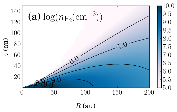
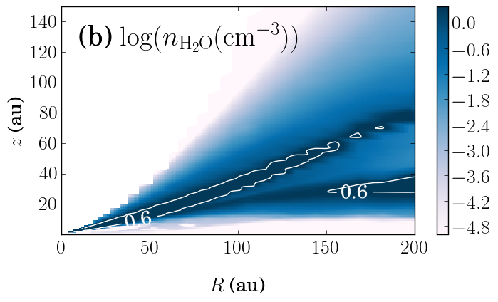
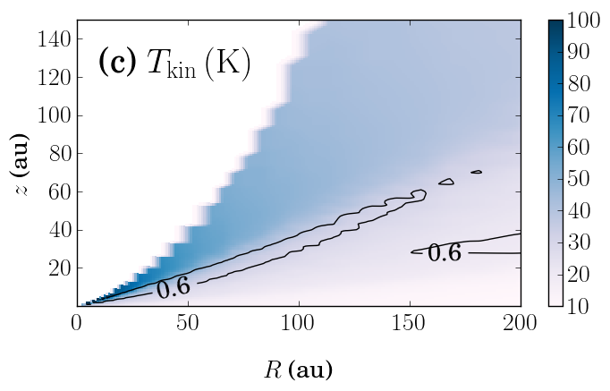
Figure 2: Overview of the adopted model structure. (a) logarithm of the molecular hydrogen density in $\rm{cm}^{-3}$ with black contours. (b) logarithm of the water vapor density with white contours at 0.6 $\rm{cm}^{-3}$. (c) shows the gas temperature, in K. Black contours represent the logarithm of the water abundance at 0.6 $\rm{cm}^{-3}$.

As Fig. 2 shows, water vapor is mostly present in a thin photo-dominated layer (models p) or near the midplane (models m) following total H₂ density profile. Figure  3 summarizes the resulting four different scenarios (Em, Ep, Cm, Cp). In all scenarios, the total amount of ammonia and water vapor is a free parameter constrained from fitting the observed line fluxes. In particular, for the p-models, this means we use the radial and vertical density distribution from the detailed calculations but scale the total amount of ammonia and water vapor up or down as necessary.

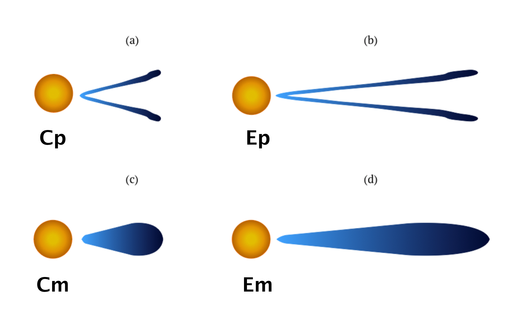
Figure 3: Schematic illustration of the location of water vapor in our models: (a) Compact photodesorption-layer configuration (Cp), (b) Extended photodesorption-layer configuration (Ep), (c) Compact with a constant abundance configuration (Cm), (d) and Extended with a constant abundance configuration (Em).

3.3 Line excitation and radiative transfer

We use LIME (v1.3.1), a non-LTE 3D radiative transfer code (Brinch & Hogerheijde, 2010) that can predict line and continuum radiation from a source model. All of our models use 15000 grid points. Doubling the number of grid points does not affect the outcome of the calculations. Grid points are distributed randomly in $R$ using a logarithmic scale. This means in practice that inner regions of the disk have a finer sampling than the outer parts of the disk. Since it is difficult to establish reliable convergence criteria, LIME requires to manually set the number of iterations of each point. We set this number to 12 confirming convergence in our models by performing consecutive iterations. Forty channels of 110 m s^-1 each are used for all line models with 200 pixels of 0.05 arcsec. Since we are comparing these models with spatially unresolved data, we calculate the total flux by summing all the pixels after subtracting the continuum.

Rate coefficients for ortho-ammonia, N₂H⁺ and both spin isomers of water are taken from the Leiden Atomic and Molecular Database (Schöier et al., 2005). The excitation levels of para-H₂O and ortho-H₂O have separate coefficients for o-H₂ and p-H₂ (Daniel et al., 2011). The o-NH₃ collision rates are only available for p-H₂, so we regard total H₂ as p-H₂ to calculate their population levels (see Danby et al., 1988). The N₂H⁺ collision rates are adopted from HCO⁺ following Flower (1999). We assume H₂ ortho-to-para ratios in local thermal equilibrium. Given the low dust temperatures this implies H₂ OPR $<0.3$. If instead we increase the H₂ ortho–to–para ratio to 3, the high temperature limit for formation on grains (Flower et al., 1996), it will increase the H₂O line fluxes increase by a factor $\sim 2$. We discuss the effect of this on the inferred water vapor mass below.

4 Results

Figure 4 shows the emerging line flux in the Herschel beam as function of ammonia and water vapor mass. These curves of growth (flux ($F$) vs mass $\propto$ column density($N$)) are consistent with saturated lines: the slopes go from linear ($F\propto N$) in the low opacity regime to saturated ($F\propto$ ${\rm\sqrt{{\rm ln}(N)}}$). The latter behavior is due to the line becoming gradually optically thick in its wings, resulting in a steady flux growth.

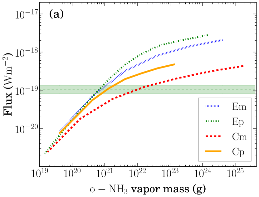
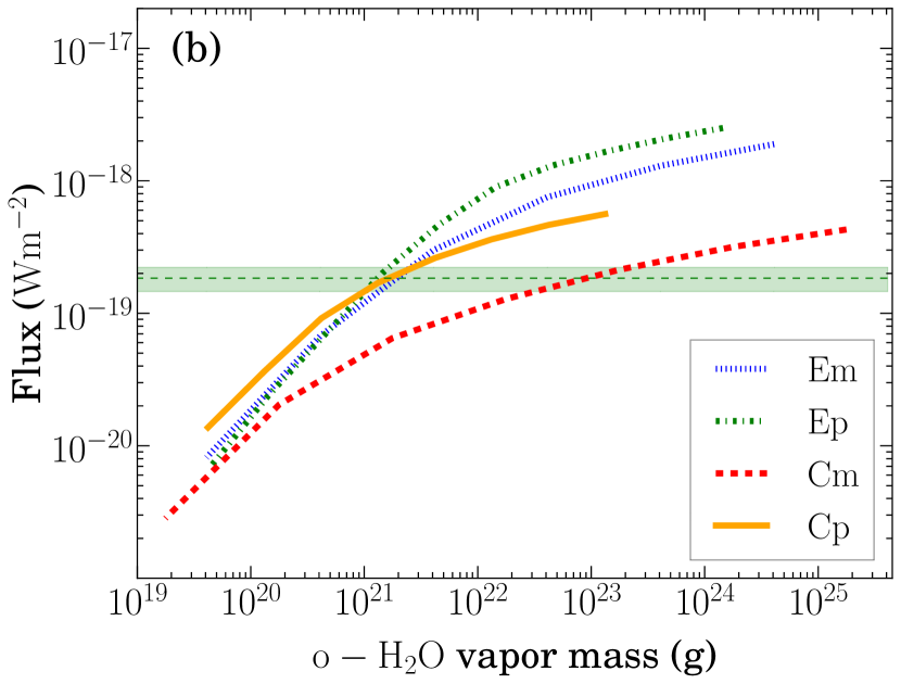
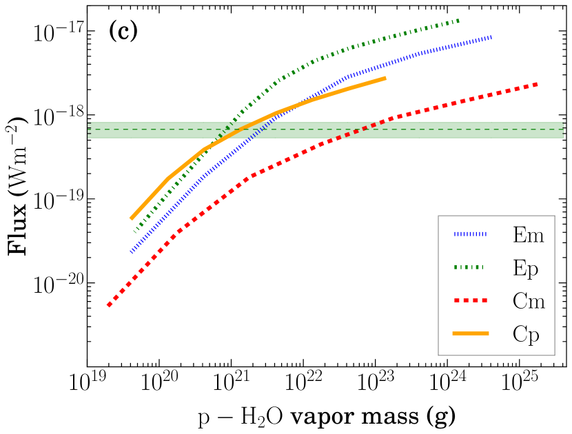
Figure 4: Figures (a), (b) and (c) shows LIME (Brinch & Hogerheijde, 2010) output of the total line fluxes of ortho-$\rm{NH_{3}}$, ortho-$\rm{H_{2}O}$ and para-$\rm{H_{2}O}$ respectively as a function of the total water vapor mass. The blue, green, red and yellow curves correspond to the Em, Ep, Cm and Cp models respectively. The dashed lines and horizontal green bar show the observed line fluxes and their 3$\sigma$ ranges, with sigma having two sources of noise added in quadrature. The systematic error of the observations, estimated to be about 20% of the total flux, and the rms of the spectra.

Our four models predict different asymptotic values for large vapor masses. In the asymptotic regimes lines are fully thick and probe only a very thin region near the surface of the disk. The larger E models therefore result in more flux compared to the smaller C models. The m models trace higher H₂ densities but lower temperatures than the corresponding p models, resulting in different predicted fluxes. This has a strong effect on the water lines, that have critical densities and upper level energies higher than the conditions prevalent in the regions where the lines originate. This effect is strongest for the Cm models because in this regime densities are considerably larger and the lines becomes thermalized and opaque, resulting in larger required water-vapor masses.

Table 2 summarizes the best-fit vapor masses; error estimates include statistical errors on the observations and the systematic errors on the total line flux, estimated to be about 20%. The ammonia to water ratios shown in Table 2 assume an OPR of ammonia of either $\infty$ or 1. As stated above in section 3.3 we assume H₂ ortho–to–para ratios in local thermal equilibrium. If we increase this value to 3 (the high temperature limit), then the derived masses would decrease by a little more than 1 order of magnitude in our most massive and optically thick model (Cm) and by less than one order of magnitude in the remaining models (Cp, Em, Ep). We do not include this in the error budget of our reported values because the NH₃ and N₂H⁺ might be equally affected.

All four models yield o-NH₃ masses ranging from (0.7–1.2)$\times 10^{21}$ g for models Ep, Em, and Cp, to 1.1$\times 10^{22}$ g. These correspond to ammonia abundances ranging from (2.0-9.5)$\times 10^{-12}$ (E models) to (0.6-1.7)$\times 10^{-10}$ (C models), relative to H₂. For water, a higher range of masses is inferred, ranging from (2.2–4.5)$\times 10^{21}$ g for models Ep, Em, and Cp, to $1.6\times 10^{23}$ g for model Cm. These correspond to water abundances ranging from (1.1-3.0)$\times 10^{-11}$ (E models) to (4.5-9.0)$\times 10^{-10}$ (C models), relative to H₂. The water OPR is found to range from 0.73 to 1.52. If the associated errors are considered then the range is much wider (0.2-3.0) with model Ep, Cp and Cm in agreement with the interstellar and cometary range of 2.0-3.0 for the OPR of water. The ammonia to water ratio ranges from 7%${}^{9\%}_{-5\%}$ to 84%${}^{61\%}_{-36\%}$.

Calculations using a simple escape-probability code (RADEX, van der Tak et al., 2007) reproduce the observed line fluxes adopting the inferred vapor masses and using densities and temperatures representative for the emitting regions. But only a full 3D calculation can reproduce the exact line fluxes because of the large range in densities and temperatures. These simple calculations also show that, under the conditions of the four models, equal amounts of o–$\rm{H_{2}O}$ and o–$\rm{NH_{3}}$ give approximately equal line strengths (within 50%). This means that we can relate the observed line ratios of $F_{\rm{o-NH_{3}}}$/$F_{\rm{o-H_{2}O}}\sim$ 0.6 to estimate the actual overall $\rm{NH_{3}/H_{2}O}$ abundance fraction of about 0.35-0.65 as confirmed by the detailed LIME modeling below. The large NH₃/H₂O ratios suggested by most models are therefore a direct consequence of the near-equal observed line fluxes of H₂O and NH₃; only in the Cm model where lines are opaque, are much lower NH₃/H₂O values consistent with the observed fluxes.

Table 2: Summary table of our results in different regimes.

	Ep	Em	Cp	Cm
Total $\rm{o-H_{2}O}$ vapor mass (1021g)	1.3${}^{+0.4}_{-0.3}$	1.9${}^{+0.6}_{-0.5}$	1.6${}^{+1.1}_{-0.6}$	94${}^{+111.2}_{-5.8}$
Total $\rm{p-H_{2}O}$ vapor mass (1021g)	0.9${}^{+0.2}_{-0.2}$	2.6${}^{+0.8}_{-0.7}$	1.4${}^{+0.7}_{-0.6}$	65${}^{+5.4}_{-3.4}$
Total $\rm{o-NH_{3}}$ vapor mass (1020g)	7.0${}^{+1.8}_{-1.9}$	8.0${}^{+0.3}_{-0.3}$	12${}^{+7}_{-4}$	110${}^{+130}_{-60}$
OPR	1.52${}^{+0.58}_{-0.49}$	0.73${}^{+0.32}_{-0.28}$	1.14${}^{+0.97}_{-0.65}$	1.38${}^{+2.07}_{-1.15}$
$\rm{NH_{3}}$/$\rm{H_{2}O}$	33%${}^{+11\%}_{-11\%}$ $\sim$ 66%${}^{21\%}_{-22\%}$	19%${}^{8\%}_{-7\%}$ $\sim$ 38%${}^{17\%}_{-15\%}$	42%${}^{30\%}_{-18\%}$ $\sim$ 84%${}^{61\%}_{-36\%}$	7%${}^{9\%}_{-5\%}$ $\sim$ 15%${}^{20\%}_{-11\%}$

Our best-fit model result for N₂H⁺ is in agreement with the N₂H⁺ 4–3 emission reported in Qi et al. (2013). The fit to the N₂H⁺ 6–5 emission yields a total N₂H⁺ vapor mass of 4.9$\times 10^{21}$ g, $\sim$50% higher than the model of Qi et al. (2013) obtained from integrating their best-fit model ($z_{\rm big}(H)=3$ in table S2).

5 Discussion

5.1 Ice reservoirs and total gass masses

The inferred NH₃ vapor masses from 7.0$\times 10^{20}$ g to 1.1$\times 10^{22}$ g are much smaller than the potential ammonia ice reservoir of $\sim 3.0\times 10^{28}$ g. This ice reservoir mass estimate was obtained assuming an elemental nitrogen abundance relative to H of $\rm{2.25\times 10^{-5}}$ and a disk mass of 0.04$\pm$0.02 M_☉, and assuming that 10% of nitrogen freezes out on grains as NH₃ (Öberg et al., 2011a). In the same way, we estimate a water ice mass reservoir of $3.4\times 10^{29}$ g, adopting an oxygen elemental abundance of $\rm{3.5\times 10^{-4}}$ relative to H, assuming that 70% of O is locked up in water (Visser et al., 2009) and all of it is frozen out. Both mass estimates indicate that the detected vapor masses are only tiny fractions ($\lesssim 10^{-6}$) of the available ice reservoirs.

The total water mass of our original chemistry model ($4.6\times 10^{24}$g) is 2.5 to 25 times (Cm and Ep models respectively) more massive than the values derived from our reanalysis of the water detection towards TW Hya. H11 reported a model 16 times more massive than their original chemistry model to fit the water emission coming from the disk of TW Hya. This value is significantly lower than the value of our analogous Ep model which indicates an even higher degree of settling of the icy grains than previously proposed. This is consistent with earlier conclusions that most volatiles are locked up in big grains near the midplane (Hogerheijde et al., 2011; Du et al., 2015).

5.2 Gas phase chemistry

The reported ammonia to water ratios are considerably higher than those found for ices in solar system comets and interstellar sources (Mumma & Charnley, 2011), which are typically below 5%. Our model derived ratios assume that the NH₃ and H₂O emission originates from the same regions; however, if this is not the case, expressing the relative amounts of ammonia and water as a ratio is not very useful. Then, it is better to work with their (disk averaged) abundances of 0.2-17.0$\times$10^-11 and 0.1-9.0$\times$10^-10 respectively.

An obvious conclusion from the large amount of NH₃ is that other routes exist for gas-phase-NH₃ in addition to evaporating NH₃/H₂O ice mixtures. In the colder outer disk the synthesis of ammonia in the gas phase relies on ion-molecule chemistry. This means that N₂ needs to be broken apart (to release N or N⁺) first, but N₂ can self-shield against photodissociation (Li et al., 2013). The chemistry in the disk of TW Hya seems to reflect an elevated X-ray state of the star (Cleeves et al., 2014). This strong X-ray field scenario could be invoked to break N₂ apart. The models of Schwarz & Bergin (2014) for a typical T Tauri disk (with a FUV field measured in TW Hya) give values for the abundance of NH₃ as high as $\sim$10^-8 (the models of Walsh et al., 2015, also produce the same abundance), which would be sufficient to explain the emission. Modeling tailored to TW Hya with the correct stellar and disk parameters, as well as appropriate initial conditions is required to fully address the question of the origin of the large NH₃ abundance.

Of our four models, the Cm model stands out in that it yields much lower NH₃/H₂O ratios that are consistent with the low values found in solar system bodies and interstellar ices. It is also the only model where the (large uncertainties of the) derived water OPR overlap with the 2-3 range commonly found in solar system comets. Recent laboratory work by (Hama et al., 2015) shows that water in ices efficiently attains an OPR of 3 upon release into the gas-phase, indicating that the OPR is not a reflection of the physical temperature and that high OPR values are naturally expected. The NH₃/H₂O values and the water OPR values together can be taken as evidence that the Cm model is a correct description for the distribution of H₂O and NH₃ in the disk. If so, a mechanism to release water in the midplane is required.

5.3 Collisions of large bodies as a production mechanism

In the midplane models (Em and Cm), photodesorption cannot explain the abundance of water and ammonia in the gas phase, as ultraviolet radiation cannot penetrate to these depths. CR-induced H2O desorption, such as modeled in H11, cannot produce the required amount of H2O. The typical water vapor abundances found in the H11 chemical model near the midplane are of order $X_{\rm{H_{2}O}}\sim 10^{-13}$, much smaller than the corresponding best-fit midplane abundances in the Em and Cm models of $X_{\rm{H_{2}O}}\sim 10^{-10}-10^{-9}$. How can volatiles such as ammonia and water exist near the midplane where low temperatures and high densities would ensure rapid freeze out?

One way of releasing such a vapor mass from the icy reservoir would be through collisions of larger icy bodies. We can calculate how much water needs to be released through these collisions, if we assume steady state with freeze out, to retain the observed amount of volatiles in the gas phase. Freeze out is calculated using the freeze-out rate expression for neutral species derived in Charnley et al. (2001). For typical temperatures of 12 K and densities of 1.7$\times 10^{9}$cm^-3, the freeze out rate of water vapor is $\rm{2.5\times 10^{13}g\leavevmode\nobreak\ s^{-1}}$ if we consider the (Em) model to match the observations. That is equivalent to completely destroying $\sim$7,000 comets per year, with a mass comparable to Halley’s comet and assuming they consist of 50% water. After 10 Myr roughly 5% of the water previously locked up in icy grains would be back to the gas phase if an ice reservoir of $\rm{3.4\times 10^{29}g}$ is present in the disk. In the case of the (Cm) model a higher production of water vapor $\rm{1.6\times 10^{16}g\leavevmode\nobreak\ s^{-1}}$ is needed to match the observations. This would mean destroying $\sim\rm{5\times 10^{6}}$ comets per year. After 10 Myr we would have produced ten times more water vapor than its total ice reservoir. Such large numbers of collisions and the significant (or even unrealistic) amount of released water suggest that collisions between icy bodies are an unlikely explanation for the observed amount of water and ammonia vapor in the midplane models.

The freeze-out rates used above have been calculated assuming a typical grain size distribution $n(a)\varpropto a^{-3.5}$ (Mathis et al., 1977) with minimum and maximum grains sizes of 10^-8 m and 10^-1 m. Since the majority of the surface for freeze-out is on (sub)$\mu$m-size grains, we can expect this surface to be substantially reduced if these smaller grains are removed thus reducing the freeze-out rate significantly. Small grains may be removed by photoevaporating winds (Gorti et al., 2015), when transported to the upper layers by vertical mixing, or have coagulated into larger grains. In the extreme case where all of the $\mu$m-size grains have grown into larger bodies the freeze-out rate can be reduced by two orders of magnitude.

We can get a drop by a factor of 100 in the freeze-out rate by directly calculating the mean grain surface in Eq.6 from Charnley et al. (2001) by setting $a_{\rm min}$=10^-4 m for our Em model, $a_{\rm min}$=10^-3m for our Cm model (see calculations of Vasyunin et al., 2011) and $a_{\rm max}$=10^-1 m for both. If this assumption holds then our model with the highest production rate (Cm) will have processed only 10% of its water reservoir into water vapor in the span of 10 Myr, equivalent to destroying only $\sim$5000 comets per year. In the same way, the amount of water processed in the span of 10 Myr in our (Em) will be only 0.5% of its ice reservoir, equivalent to destroying only $\sim$70 comets per year. Such number are much more realistic, making this a viable mechanism to release volatiles in the midplane.

Nevertheless, for this scenario to be viable, the system must meet some criteria. First, the comets (or planitesimals) must have a high enough collision rate that accounts for the numbers estimated above. In the outer disc this can be enhanced through shepherding by planets, i.e., sweeping up the planetesimals into one proto-debris belt. Acke et al. (2012) calculate a collision rate of $\rm{6.3\times 10^{13}g\leavevmode\nobreak\ s^{-1}}$ in Fomalhout’s debris disk to reproduce the thin dust belt seen in far-infrared images (70-500 $\mu m$). This rate is comparable to our estimated rate even in the absence of a reduction in grain surface available for freeze out. In the case of Fomalhout, this rate corresponds to a population of $\rm{2.6\times 10^{11}}$ 10-km-sized comets comparable to the number of comets in the Oort Cloud of $\rm{10^{12}-10^{13}}$ (Weissman, 1991). Second, the collisions must release enough energy to sublimate the ices. This is only achieved if the relative velocities of the parent bodies are sufficiently high. If the colliding bodies have high eccentricities their relative velocities can be large. But in the presence of gas, we expect their orbits to be circularised. If this is the case, then the relative velocities will be dominated by the radial drift in the outer parts of the disk and enhanced in the very inner regions by turbulence. Finally, the small dust produced in the cometary (or planitesimal) collisions themselves must not provide a surface for the volatiles to freeze back onto.

If a sufficient number of small grains ($\lesssim\mu$m) is removed by coagulation into larger grains ($\gtrsim$ mm) and the relatives velocities and rates of the collisions between larger bodies ($\gtrsim$ m) in the miplane are sufficiently high to meet the conditions above, then collisions between icy bodies is a plausible mechanism to release (and keep in the gas phase for long enough) the amount of water and ammonia that we observe. The treatment above is simplistic and there are many other ways to achieve this (e.g., changing the slope of the grain distribution or by photoevaporation of grains along with the gas). A full treatment of the combined effect of grain growth, drift, settling, collisions and volatile freeze-out is needed to confirm this scenario but is beyond the scope of this paper.

6 Conclusions

We have successfully detected NH₃ and N₂H⁺ in the disk surrounding TW Hya. We use a non-LTE excitation and radiative transfer code and a detailed physical and chemical disk structure to derive the amount of NH₃, N₂H⁺, and (for comparison) H₂O adopting four different spatial distributions of the molecules. Our main conclusions are as follows.

1. The NH₃ emission corresponds to an ammonia vapor mass that ranges from $7.0\times 10^{20}$g (Ep model) to $1.1\times 10^{22}$g (Cm model).

2. We use the above values and the same approach to get H₂O vapor masses to derive NH₃/H₂O ratios ranging from 7% to 15% (Cm model) and 42% to 84% (Cp model), adopting a NH₃ OPR of $\infty$ or 1, respectively. These ratios are higher than those observed in solar system and interstellar ices, with the exception of our most massive and compact configuration (Cm model).

3. Of our four models, only model Cm gives NH₃/H₂O ratios as low as observed in interstellar ices and solar system comets. It is also the only model that, within the errors, gives a water OPR of 2-3 comparable to solar system comets. This can be taken as evidence that H₂O and NH₃ are indeed located near the midplane at at radii $<$60 au.

4. If the H₂O and NH₃ follow the Cp, Ep, or Em spatial distributions, the implied high NH₃/H₂O ratio requires an additional mechanism to produce gas-phase NH₃. A strong X-ray field may provide the necessary N atoms or radicals to form NH₃ in the gas.

5. If NH₃ and H₂O emission comes from the midplane, where photodesorption does not operate (models m), collisions of larger bodies can release NH₃ and H₂O and explain the observed vapor. This requires a reduction of the total grain surface available for freeze out, e.g., through the growth of grains into pebbles and larger; and a sufficiently high collision rate and sufficiently violent collisions to release the volatiles.

6. The ammonia vapor mass is similar to the N₂H⁺ mass derived with our simple model and to that inferred by Qi et al. (2013) (see section 4) within 50%.

Additional spatially resolved observations of ammonia would help to constrain the radial extent of ammonia (and perhaps vertical structure) and refine our current limits. We can observe ammonia isotopes with ALMA in Band 7 (ortho-NH₂D $1_{01}-0_{00}$ at 332.781 GHz and para-NH₂D $1_{01}-0_{00}$ at 332.822 GHz) and Band 8 (ortho-NH₂D $1_{10}-0_{00}$ at 470.271 GHz and para-NH₂D $1_{10}-0_{00}$ at 494.454 GHz). We used our models to predict line fluxes of about 1 Jy in band 8 and 30 mJy in band 7 using LIME in all of our models, and considering a value of 0.1 for ammonia deuterium fractionation as found towards protostellar dense cores (Roueff et al., 2005; Busquet et al., 2010) and a OPR ammonia of 1. ALMA can detect such line fluxes in a couple of hours OA. Observations with JVLA or GBT of para-ammonia (para-NH₃ $1_{1}-1_{0}$ at 23.694 GHz or para-NH₃ $2_{1}-2_{0}$ at 23.722 GHz) are not possible since our predicted line fluxes are too small ($\sim$ 10 mJy).