Abstract.

This paper focuses on a data-rich environment where the data set has a very large cross-sectional dimension, is likely to exhibit local dependence, and yet is hard to determine the dependence ordering. Such a situation arises, for example, when the data set is collected from the Internet, through a method of web crawling. This paper proposes an approach of randomized subsampling inference, where one constructs a test statistic by aggregating many randomized test statistics using random draws of subsamples, and uses for inference the conditional distribution of the test statistic given data. This paper explores two approaches of such inference: one based on an M-type statistic constructed from randomized mean statistics and the other based on a U-type statistic constructed from randomized U-statistics. This paper provides conditions for local dependence, the number of the random draws, and the subsample size, under which randomized subsampling inference is asymptotically valid. From the Monte Carlo simulation studies, this paper finds that the randomized subsampling inference based on the U-type statistics performs better than that based on the M-type statistics.

Key words. Randomized Subsampling Inference; Local Dependence; Cross-Sectional Dependence; Ordering-Free Inference; Randomized Tests
 

JEL Classification: C01, C12, C13

At Google, for example, I have found that random samples on the order of 0.1 percent work fine for analysis of business data.

Varian (2014)

1. Introduction

Collecting data from the Internet has recently been among the common practices in empirical research. Typically, such data sets have a huge cross-sectional dimension, and are collected using a sampling scheme that is far from random sampling. The sampling often relies on various methods of web crawling where a computer code automatically searches through numerous websites following a set of protocols. In this set-up, if one simply assumes that the observations are i.i.d., the inference may give nearly zero standard errors, making it irrelevant to perform statistical inference. (See Granger (1988).) On the other hand, incorporating a dependence structure in statistical inference is far from trivial due to the use of a non-random sampling scheme often consisting of complex, and ad hoc protocols.

The issue with unknown dependence ordering is not confined to such online data. For example, if the cross-sectional units are people in a social network, their observed actions are likely to be correlated, but it is hard for the researcher to determine the very network which shapes the cross-sectional dependence ordering of the observations. Another example is a situation where the cross-sectional units are differentiated products and observations are their sales in the market. Due to substitutability among the products, the sales should be correlated, and yet, the precise substitution pattern of the products is notoriously hard to determine from data.

To the best of the author’s knowledge, there does not exist a method of formal statistical inference that is generally available in such a situation. The existing methods of asymptotic inference based on normal approximation do not apply, because it is not possible to make the test statistic asymptotically pivotal without knowing the pattern of local dependence ordering. Inference based on various existing bootstrap methods such as nonparametric bootstrap, residual-based bootstrap or multiplier bootstrap does not apply here. The method of subsampling does not apply either, because without properly incorporating the dependence pattern in the subsamples, there is no way the distribution of subsamples can imitate the distribution of the whole sample.

In such a situation, this paper proposes using what this paper calls randomized subsampling inference. The main idea is to construct a randomized test statistic by aggregating random subsamples. Randomized subsampling inference is a general idea which is easy to use. It is ordering-free inference in the sense that it enables one to perform statistical inference without committing oneself to a particular model of the way cross-sectional dependence ordering arises among the sample units. For example, suppose that the cross-sectional observations have the same mean and we are interested in testing whether the mean is zero or not. For each randomly drawn subsample, we construct a two-sided t-test statistic. To enhance the power of the test, we build a randomized test statistic by aggregating such t-test statistics. Finally, one constructs many such randomized test statistics and uses their empirical distribution to construct critical values.

The intuition behind this approach is straightforward. As long as the cross-sectional dimension is high and the dependence is local (in the sense that each cross-sectional unit has only a small set of other units that it is strongly correlated with), the observations in each subsample will be likely to be nearly independent, and under proper conditions, this independence will be maintained even after a certain level of aggregation of those subsamples, regardless of what dependence ordering the local dependence of the original observations follows. Hence the distribution of the randomized test statistic may be approximated by a distribution in a way that does not invoke knowledge of the local dependence ordering.

The main goal of this paper is to formally study the method of randomized subsampling inference, focusing on the simple task of testing for the population mean, though the results can be directly extended to more general set-ups. As a first step, this paper formalizes the notion of local dependence in a way that is proper to this type of study. This paper introduces a local dependence measure that is ordering-free in the sense that the set of observations has the same local dependence measure as any permutation of the observations. Roughly speaking, the local dependence measure is based on the likelihood that any randomly chosen small subset of observations turn out to be strongly dependent with one another. When the observations are dependent only locally, this likelihood should be small, yielding a low measure of local dependence. As shown in this paper, a bound for the ordering-free measure of local dependence can be derived from various notions of temporal and spatial weak dependence such as strong mixing time series or random fields, $m$-dependent series, observations with a dependency graph, and observations with a group-dependence structure such that within-group dependence is permitted but between-group dependence is not.

This paper studies two approaches of constructing a test statistic. The first approach uses an M-type statistic which is based on the sample mean of randomized subsamples. The second approach uses a U-type statistic which is based on the U-statistic of randomized subsamples. The main results of this paper are two-fold. First, we establish conditions for local dependence, the number of the randomly drawn subsamples, and the subsample sizes such that the test statistics constructed without knowledge of local dependence ordering are asymptotically pivotal. Second, we introduce the notion of rate-dominance with size control to compare the two approaches. The comparison is not trivial because their size properties are potentially different. This rate-dominance result compares the two approaches in terms of power after the size is controlled up to a higher order term. This paper shows that the U-type statistic approach rate-dominates the M-type statistic approach when permutation-based critical values are used.

This paper studies the performance of the two types of the test statistics through Monte Carlo simulations. The Monte Carlo study considers two types of local dependence; dependency graph and approximate dependency graphs. The study finds the superior performance of randomized subsampling inference based on the U-type statistic approach. In particular, as compared to the normal approximation, it performs more stably across a wide range of local dependence configurations. When the finite sample size is controlled, using the U-type statistic shows higher power than using the M-type statistic.

There are two potential drawbacks of the randomized subsampling inference approach. First, the randomness of the test statistic in the use of inference is primarily from the randomness of the randomized subsamples, which means that given the same sample, the method can yield two different results though with a small probability. To overcome this issue, one may perform randomized inference many times and report the distribution of such results. More specifically, this paper follows Geyer and Meeden (2005) and proposes what it calls a randomized confidence function which traces out the average non-rejection probabilities of many randomized tests across different parameter values. Another potential limitation comes from the fact that the convergence rate of the randomized subsampling inference is slower than the convergence rate of the estimation (e.g. the convergence rate of the sample mean). This paper regards the slower rate as a price to pay for performing inference that is robust to any form of local dependence ordering. When the cross-sectional dimension is high, some loss of power in statistical inference to gain more robustness may not be so detrimental.

Literature Review: The early literature of robust inference under weak dependence and heteroskedasticity has focused on consistent estimation of asymptotic covariance matrix (White (1980), Newey and West (1987) and Andrews (1991)). A more recent strand of literature uses inconsistent scale normalizer that uses a fixed smoothing parameter (Kiefer, Vogelsang, and Bunzel (2000) and Kiefer and Vogelsang (2002)). For example, Phillips, Sun, and Jin (2007) and Sun, Phillips, and Jin (2011) considered power kernels. Jansson (2004) and Sun, Phillips, and Jin (2008) explored higher order accuracy of fixed smoothing asymptotics over increasing smoothing asymptotics. Sun (2014) established related results in a more general context of two-step GMM estimation. In the meanwhile, Müller (2007) showed non-robustness of HAC estimators to local perturbations of the DGP and proposed a class of quadratic long-run variance estimators. Sun and Kim (2015) proposed asymptotic F tests based on fixed smoothing asymptotics in the GMM framework with weakly dependent random fields. Also apart from this econometrics literature, it is worth noting that Shao and Politis (2013) applied the fixed smoothing approach to subsampling inference that uses a calibration method.

Robust estimation of asymptotic covariance matrix has received a great deal of attention in the literature of linear panel models and spatial models as well. Arellano (1987) proposed HAC estimation in linear panel models with fixed effects. Driscoll and Kraay (1998) suggested a simple approach of HAC estimation in linear panel models based on cross-sectional averages of moment functions. Vogelsang (2012) compares the two approaches using fixed smoothing asymptotics. See also Kelejian and Prucha (2007) and Kim and Sun (2011) for HAC estimation in spatial models.

A closely related approach in dealing with cross-sectional dependence is linear or nonlinear modeling of spatial autoregressive models and the approach of clustered errors. (See Lee (2004), and Lee, Liu, and Lin (2010) for contributions to the literature of spatial autoregressive models, among many others, and references therein.) As for models with clustered errors, Cameron, Gelbach, and Miller (2008) proposed and studied bootstrap approaches to deal with clustered errors. This literature typically assumes many independent clusters in a linear set-up. Ibragimov and Müller (2010) proposed a novel approach based on t-statistics where the observations are divided into multiple clusters that are (approximately) independent from each other and the inference is based on within-cluster estimators that are asymptotically normal. Bester, Conley, and Hansen (2011) elaborated this multiple-cluster approach in linear panel models and provided conditions that are more primitive than those of Ibragimov and Müller (2010). The t-statistic approach of Ibragimov and Müller (2010) allows for the clusters to be few and to be heterogeneous on various dimensions such as size or within-cluster dependence strength. However, the approach requires knowledge of this group structure of (at least approximately) independent clusters.

A strand of literature has focused on developing tests for cross-sectional dependence using mainly cross-sectional variations. Pesaran (2004) developed a general test for cross-sectional dependence in linear panel models with a short time series dimension. See also Hsiao, Pesaran, and Pick (2012) for an extension to limited dependent models. Robinson (2008) proposed a correlation test that can be applied for testing cross-sectional dependence in a spatial model. Kuersteiner and Prucha (2013) considered a linear panel model with a large cross-sectional dimension which does not require a long time series. Adopting a sequential exogeneity condition, and assuming conditional moment type restrictions, they obtained a limit theory for GMM estimators that accommodate unknown common shocks and various latent cross-sectional dependence structures. (See also Kuersteiner and Prucha (2015) for a more general framework which includes linear quadratic moment restrictions in dynamic panel models which accommodate social interactions and networks models.)

The use of permutations and subsamples in this paper is different from permutation tests and subsampling-based inference in the literature. Most importantly, the main use of permutations or subsamples in this paper is for constructing test statistics rather than for finding critical values. It is more like a Monte Carlo test than a standard permutation test. Also, randomized subsampling inference is fundamentally different from the subsampling inference of Politis and Romano (1994). Here, subsamples are used primarily to construct a test statistic rather than critical values.

Using randomly drawn subsamples for data analysis is a common practice in empirical research when the data set size is huge. (See Varian (2014).) A closely related approach is bootstrap aggregating (or bagging) proposed by Breiman (1996) which is used to obtain stable predictions using many bootstrap samples. Recently Kleiner, Talwalker, Sarkar, and Jordan (2014) proposed using random subsamples to measure the quality of the estimates adn showed the measure is consistent as the subsample size increases to infinity. The main motivation for their proposal is to reduce the computational costs when the sample size is large. Unlike their approach, the focus here is on inference with observations that are locally dependent but the dependence ordering is not known to the researcher. It does not seem to have received attention in the literature that using randomly drawn subsamples one may obtain inference that is robust to a wide range of configurations of local dependence ordering.

Organization of the Paper: Section 2 introduces the main idea of randomized subsampling inference, ordering-free local dependence measure, and illustrates its meaning through examples. The section also establishes conditions for asymptotic validity, and provide results that compare the M-type statistic and the U-type statistic approaches through the notion of rate-dominance with size control. In Section 3, this paper presents and discusses results from a Monte Carlo simulation study. Technical proofs of part of the main results are found in the appendix. Supplemental Note to this paper contains extension to inference from moment-based restrictions and proofs of the other results in the paper.

2. Randomized Subsampling Inference on the Mean

2.1. The Basic Set-Up

Consider the simple set-up of estimating the population mean from locally dependent data. Suppose that we are given observed random vectors $X_{1,n},...,X_{n,n}\in\mathbf{R}^{d}$ and a (potentially latent) common shock $\mathcal{C}_{n}$ such that

$$\mathbf{E}[X_{i,n}]=\mathbf{E}[X_{i,n}|\mathcal{C}_{n}],$$

for all $i\in\{1,...,n\}$. Thus we assume that $X_{i,n}$ is conditionally mean independent of the common shock $\mathcal{C}_{n}$. Let us assume that $X_{i,n}$’s have the same mean:

$$\mu_{0}\equiv\mathbf{E}X_{i,n}.$$

The main goal here is to develop a procedure to yield an asymptotically valid confidence set for $\mu_{0}$ as the sample size $n$ goes to infinity. For this, consider the following testing problem of null and alternative hypotheses.

$$H_{0}:\mu_{0}=\bar{\mu},\textnormal{ against }$$

$$H_{1}:\mu_{0}\neq\bar{\mu},$$

for a given vector $\bar{\mu}$.

Without knowing the local dependence ordering, it is not possible to use the usual t-statistic. The t-statistic (in the case of $d=1$) takes the following form:

$$\left|\frac{\sqrt{n}\overline{X}_{n}}{\hat{\sigma}}\right|,$$

where $\overline{X}_{n}=\frac{1}{n}\sum_{i=1}^{n}X_{i,n}$ and $\hat{\sigma}^{2}$ is a consistent estimator of $\sigma^{2}$ such that

$$\sqrt{n}(\overline{X}_{n}-\mu_{0})\rightarrow_{d}N(0,\sigma^{2}).$$

The difficulty here is that without knowing which observations are strongly correlated with $X_{i,n}$ for each $i\in\{1,...,n\}$, it is hard to find a consistent estimator of $\sigma^{2}$. In fact, we can write

$$\sigma^{2}=\lim_{n\rightarrow\infty}\sigma_{n}^{2},$$

where

$$\sigma_{n}^{2}=\frac{1}{n}\sum_{i=1}^{n}\text{Var}(X_{i,n})+\frac{1}{n}\sum_{i=1}^{n}\sum_{j=1:j\neq i}^{n}\text{Cov}(X_{i,n},X_{j,n}).$$

Under local dependence, one can consistently estimate the leading term in the definition of $\sigma_{n}^{2}$ without knowledge of dependence ordering. The problem is the second term for which, to the best of the author’s knowledge, there is no existing method to consistently estimate it without knowing which set of $X_{j,n}$’s are nearly uncorrelated with $X_{i,n}$ for each $i$. Thus performing statistical inference without knowing local dependence ordering is fundamentally a nontrivial task, even for this simple testing problem for a population mean.

2.2. Two Approaches of Randomized Subsampling Inference

2.2.1. The M-Type Statistic Approach

Let $\Pi$ be the set of permutations on $\{1,...,n\}$ and $\pi_{1},...,\pi_{R}$ be i.i.d. draws from the uniform distribution on $\Pi$. Given each $\pi_{r}\in\Pi$, $r=1,...,R_{n}$, and $\bar{\mu}\in\mathbf{R}^{d}$, we define

$$M_{n}(\bar{\mu};\pi_{r})=\frac{1}{\sqrt{db_{n}}}\sum_{i=1}^{b_{n}}{\hat{\Sigma}}^{-1/2}\left(X_{\pi_{r}(i),n}-\bar{\mu}\right),$$

where

(2.1) $$\hat{\Sigma}=\frac{1}{n}\sum_{i=1}^{n}(X_{i,n}-\overline{X}_{n})(X_{i,n}-\overline{X}_{n})^{\prime},$$

and $b_{n}\leq n$. We call $\{X_{\pi_{r}(i),n}\}_{i=1}^{b_{n}}$ a randomized subsample and the number $b_{n}$ the subsample size. A randomized subsample is obtained by first permuting the sample $\{X_{i,n}\}_{i=1}^{n}$ using a permutation randomly drawn from $\Pi$ and by taking the first $b_{n}$ observations from the permuted sample. The normalization by the covariance matrix $\hat{\Sigma}$ controls only for the “short-run” covariance among the entries of the random vector $X_{i,n}$, not the cross-sectional dependence. Then we define

$$S_{M,n}(\bar{\mu};\boldsymbol{\pi})=\left\|\frac{1}{\sqrt{R_{n}}}\sum_{r=1}^{R_{n}}M_{n}(\bar{\mu};\pi_{r})\right\|^{2},$$

where $\boldsymbol{\pi}=(\pi_{1},...,\pi_{R_{n}})$ and $||a||^{2}=a^{\prime}a$ for a vector $a$. We introduce the test statistic as follows:

$$T_{M,n}(\bar{\mu};\boldsymbol{\pi})=S_{M,n}(\bar{\mu};\boldsymbol{\pi})-\frac{R_{n}b_{n}}{n}.$$

The additive term $R_{n}b_{n}/n$ is a bias adjustment term which we will explain later.

Let us consider the following method of constructing a critical value. For given $L$, we draw $\boldsymbol{\pi}_{l}$, $l=1,...,L$, i.i.d., where $\boldsymbol{\pi}_{l}=(\pi_{1,l},...,\pi_{R_{n},l})$ and $\pi_{r,l}$’s are i.i.d. draws from the uniform distribution on $\Pi$. Define for $\alpha\in(0,1)$,

$$c_{M,\alpha}=\inf\left\{c>0:\frac{1}{L}\sum_{l=1}^{L}1\left\{S_{M,n}(\bar{\mu};\boldsymbol{\pi}_{l})>c\right\}\leq\alpha\right\}.$$

In other words, the critical values are read from the $1-\alpha$ percentile of the empirical distribution of $\{S_{M,n}(\bar{\mu};\boldsymbol{\pi}_{l})\}_{l=1}^{L}$. Note that we use the sample mean $\overline{X}_{n}$ in place of $\bar{\mu}$ to ensure that the test may have power when $\mu_{0}\neq\bar{\mu}$.

2.2.2. The U-Type Statistic Approach

As before, let $\Pi$ be the space of permutations on $\{1,...,n\}$ and $\pi_{1},...,\pi_{R}$ be i.i.d. draws from the uniform distribution on $\Pi$. Given $\pi_{r}\in\Pi$ and $\bar{\mu}\in\mathbf{R}^{d}$, we define

$$U_{n}(\bar{\mu};\pi_{r})=\frac{1}{db_{n}}\sum_{i,j=1:i\neq j}^{b_{n}}\left(X_{\pi_{r}(i),n}-\bar{\mu}\right)^{\prime}{\hat{\Sigma}}^{-1}\left(X_{\pi_{r}(j),n}-\bar{\mu}\right),$$

where $\hat{\Sigma}$ is as defined in (2.1), and let

$$S_{U,n}(\bar{\mu};\boldsymbol{\pi})=\frac{1}{\sqrt{R_{n}}}\sum_{r=1}^{R_{n}}U_{n}(\bar{\mu};\pi_{r}).$$

We introduce the test statistic as follows:

$$T_{U,n}(\bar{\mu};\boldsymbol{\pi})=S_{U,n}(\bar{\mu};\boldsymbol{\pi})-\frac{\sqrt{R_{n}}(b_{n}-1)}{n}.$$

Again, the term $\sqrt{R_{n}}(b_{n}-1)/n$ is a bias adjustment term.

For given $L$, we draw $\boldsymbol{\pi}_{l}$, $l=1,...,L$, i.i.d., similarly as before, where $\boldsymbol{\pi}_{l}=(\pi_{1,l},...,\pi_{R_{n},l})$ and $\pi_{r,l}$’s are i.i.d. draws from the uniform distribution on $\Pi$. Define for $\alpha\in(0,1)$,

$$c_{U,\alpha}=\inf\left\{c>0:\frac{1}{L}\sum_{l=1}^{L}1\{S_{U,n}(\overline{X}_{n};\boldsymbol{\pi}_{l})>c\}\leq\alpha\right\}.$$

2.3. Ordering-Free Local Dependence Measure

We first formulate the notion of “locality” in local dependence without invoking dependence ordering. The main idea in this paper is to measure the locality by quantifying the likelihood that a random selection of a small subset of $\{X_{i,n}\}_{i=1}^{n}$ gives a set that is partitioned into two nearly independent subsets. If the likelihood is large, the underlying dependence is deemed local. This notion of locality does not invoke any underlying dependence ordering.

To formalize this intuition, suppose that for any subset $A\subset\{1,2,...,n\}$, $c_{n}(A)$ measures the strength of the joint conditional dependence of $X_{A,n}=(X_{i,n})_{i\in A}$ given a common shock $\mathcal{C}_{n}$. We will introduce one definition of $c_{n}(\cdot)$ later. Then, the ordering-free local dependence measure of the triangular array $\{X_{i,n}\}_{i=1}^{n}$ is defined as follows: for each $k\in\{1,...,n\}$,

(2.2) $$\lambda_{n}(k)=\frac{1}{|\Pi|}\sum_{\pi\in\Pi}c_{n}(\{\pi(1),...,\pi(k)\}).$$

The local dependence of a large set of observations is measured by the convergence rate of $\lambda_{n}(k)$ (with each fixed $k$) to zero as the sample size $n$ goes to infinity. We call $\lambda$ the $\lambda$-coefficient of $\{X_{i,n}\}_{i=1}^{n}$ (with respect to a given common shock $\mathcal{C}_{n}$). The $\lambda$-coefficient is ordering-free. Indeed, two triangular arrays $\{X_{i,n}\}_{i=1}^{n}$ and $\{Y_{i,n}\}_{i=1}^{n}$ have the same $\lambda$-coefficient if $X_{i,n}=Y_{\pi(i),n}$ for all $i\in\{1,...,n\}$, for some $\pi\in\Pi$.

Let us introduce $c_{n}(\cdot)$. First, let for each $A\subset\{1,...,n\}$

$$\mathcal{P}(A)\equiv\left\{\{A_{1},A_{2}\}:A_{1}\cup A_{2}=A,A_{1}\cap A_{2}=\varnothing,\textnormal{ and }A_{1},A_{2}\neq\varnothing\right\},$$

i.e., the collection of the sets $\{A_{1},A_{2}\}$ of two nonempty subsets $A_{1},A_{2}$ of $\{1,...,n\}$ which constitute a partition of $A$. Let $\mathcal{F}$ be the union of $\mathcal{F}_{l}$’s over $l\in\{1,...,n\}$, where $\mathcal{F}_{l}$ is a given class of real measurable functions on $\mathbf{R}^{ld}$. (For this paper’s proposal, it suffices to take the class of functions $\mathcal{F}_{l}$ as a finite set of eighth-order polynomials. See a remark prior to Assumption 2.1 below.) For each $A\subset\{1,2,...,n\}$, we take

$$c_{n}(A)=\underset{\{A_{1},A_{2}\}\in\mathcal{P}(A)}{\min}c_{n}(A_{1},A_{2}),$$

where

$$c_{n}(A_{1},A_{2})=\sup_{(f_{1},f_{2})\in\mathcal{F}_{|A_{1}|}\times\mathcal{F}_{|A_{2}|}}\left|Corr\left(f_{1}(X_{A_{1},n}),f_{2}(X_{A_{2},n})|\mathcal{C}_{n}\right)\right|,$$

and $Corr(X,Y|\mathcal{C}_{n})$ represents the conditional (Pearson) correlation coefficient between $X$ and $Y$ given $\mathcal{C}_{n}$ if $Var(X|\mathcal{C}_{n})Var(Y|\mathcal{C}_{n})>0$ and zero otherwise. (The minimum over an empty set in the above expression is taken to be one.) For example, when there exists $i\in A$ such that $X_{i,n}$ is conditionally independent of $\{X_{j,n}:j\in A\backslash\{i\}\}$ given $\mathcal{C}_{n}$, we have $c_{n}(A)=0$. Hence when $X_{i,n}$’s are conditionally independent, $\lambda_{n}(k)=0$, for any $k\geq 1$.

The notion of $\lambda$-coefficient here is inspired by $\psi$-weak dependence notion proposed by Doukhan and Louhichi (1999) for time series. The major distinction is that the dependence measure is made invariant to the permutations of the observations, making unnecessary any reference to the underlying dependence ordering.

Example 1: Triangular Arrays with a Dependency Graph Let a graph $G_{n}=(\{1,...,n\},E_{n})$ over $\{1,...,n\}$ be given, where $E_{n}$ denotes the collection of pairs $ij$, with $i,j\in\{1,...,n\},$ representing an edge (or a link) between vertices (or nodes) $i$ and $j$. We exclude loops, i.e., for all $ij\in E_{n}$, $i\neq j$. Let us assume that the graph is undirected so that whenever $ij\in E_{n}$, $ji\in E_{n}$. Let $(X_{i,n})_{i=1}^{n}$ be a given triangular array of random variables. Let us say that $G_{n}$ is a conditional dependency graph for $(X_{i,n})_{i=1}^{n}$ given a $\sigma$-field $\mathcal{C}_{n}$, if for any two subsets $A_{1}$ and $A_{2}$ of $\{1,...,n\}$ such that $\{ij\in E_{n}:i\in A_{1},j\in A_{2}\}=\varnothing$, $(X_{i,n})_{i\in A_{1}}$ and $(X_{i,n})_{i\in A_{2}}$ are conditionally independent given $\mathcal{C}_{n}$. (See e.g. Penrose (2003), p.22.)

The case of a triangular array with a dependency graph having a bounded maximum degree includes $m$-dependent time series as a special case. Also dependence with clusters, where there is a partition of the observations into clusters and dependence is restricted to within-cluster observations, not between clusters, is a special case of local dependence with a dependency graph.

A simple combinatoric argument gives a bound for the $\lambda$-coefficient of the triangular array $(X_{i,n})_{i=1}^{n}$. (The proof is found in Supplemental Note.)

Lemma 2.1.

Suppose that $\{X_{i,n}\}_{i=1}^{n}$ is a triangular array of random variables having $G_{n}=(\{1,...,n\},E_{n})$ as a conditional dependency graph given $\mathcal{C}_{n}$.

Then for each integer $k\geq 2$, there exist $C_{k}>0$ and $n_{k}\geq 1$ depending only on $k$ such that for all $n\geq n_{k}$,

$$\lambda_{n}(k)\leq C_{k}n^{-k+1}d_{n}^{k-1},$$

where $d_{n}$ denotes the maximum degree of $G_{n}$.

Suppose that $d_{n}$ is bounded. Then at any fixed $k\geq 2$, the $\lambda$-coefficient converges to zero as $n\rightarrow\infty$ at the rate of $n^{-k+1}$. The bound in Lemma 2.1 is conveniently simple, as it depends on the graph through only its maximum degree. It is possible to obtain a more sophicated bound that involves other features of the network.

Example 2: Weakly Dependent Random Fields Suppose that a random field $(Y_{j,n})_{j\in\mathbb{Z}^{\prime}_{d}}$ is given, where $\mathbb{Z}^{\prime}_{d}$ is a subset of $\mathbb{Z}_{d}$ such that $n=|\mathbb{Z}_{d}^{\prime}|$ and $\mathbb{Z}_{d}$ is a lattice as a subset of $\mathbf{R}^{d}$. For each pair $(j_{1},j_{2})\in\mathbb{Z}_{d}\times\mathbb{Z}_{d}$, we define distance $d(j_{1},j_{2})=\max_{1\leq k\leq d}|j_{1,k}-j_{2,k}|$, where $j_{1,k}$ and $j_{2,k}$ are the $k$-th entry of $j_{1}$ and $j_{2}$ respectively. We assume that the lattice $\mathbb{Z}_{d}$ is infinite countable having $d_{0}>0$ such that for all $j_{1},j_{2}\in\mathbb{Z}_{d}$, we have $d(j_{1},j_{2})\geq d_{0}$. Hence as in Conley (1999) and Jenish and Prucha (2009a), we exclude the infill asymptotics where the sampling points become dense in a given domain as the sample size increases.

To map the random field to a triangular array, let $\mu:\{1,...,n\}\rightarrow\mathbb{Z}^{\prime}_{d}$ be a one-to-one map, so that we let $X_{i,n}=Y_{\mu(i),n}$, $i=1,...,n$, and define $d_{\mu}(i,j)=d(\mu(i),\mu(j))$ for simplicity. Also, for given subsets $A,A^{\prime}$ of $\{1,...,n\}$, let

$$d_{\mu}(A,A^{\prime})=\underset{i\in A,j\in A^{\prime}}{\min}d(\mu(i),\mu(j)).$$

For simplicity, let us assume that there is no common shock. Define for $m\geq 0$,

$$\bar{c}_{m,n}(A)=\min_{\{A_{1},A_{2}\}\in\mathcal{P}(A):m\leq d_{\mu}(A_{1},A_{2})<m+1}c_{n}(A_{1},A_{2}).$$

Hence $\bar{c}_{m,n}(A)$ measures stochastic dependence among $X_{i,n}$’s with $i\in A$, when there exists a partition $(A_{1},A_{2})$ of $A$ such that $m\leq d_{\mu}(A_{1},A_{2})\leq m+1$. The following lemma characterizes a bound for the $\lambda$-coefficient of $\{X_{i,n}\}_{i=1}^{n}$ in terms of $\bar{c}_{m,n}(A)$. (The proof is found in Supplemental Note.)

Lemma 2.2.

Suppose that $(Y_{j,n})_{j\in\mathbb{Z}^{\prime}_{d}}$ is a random field and let $X_{i,n}=Y_{\mu(i),n}$, $i=1,...,n.$ Suppose further that for some $q\geq 2$, and for each integer $2\leq k\leq q$, there exists $C_{k,d}>0$ such that

(2.3) $$\sum_{m=1}^{\infty}m^{(k-1)(d-1)}\max_{\pi\in\Pi}\bar{c}_{m,n}(\{\pi(1),...,\pi(k)\})\leq C_{k,d},\textit{ for all }n\geq 1.$$

Then, for each integer $2\leq k\leq q$, there exist $C_{k,d}^{\prime}>0$ and $n_{k,d}\geq 1$ such that

$$\lambda_{n}(k)\leq C_{k,d}^{\prime}n^{-k+1},\textit{ for all }n\geq n_{k,d},$$

where $C_{k,d}^{\prime}$ and $n_{k,d}$ are constants depending only on $k,d$ and $C_{k,d}$.

When the random field is a strong-mixing random field, the condition (2.3) can be verified in terms of the strong-mixing coefficient. To see this, define

(2.4) $$\alpha(A_{1},A_{2})=\sup_{i\in A_{1}}\sup_{j\in A_{2}}\alpha(\sigma(X_{i,n}),\sigma(X_{j,n})),$$

where $\alpha(\sigma(X_{i,n}),\sigma(X_{j,n}))$ denotes the strong mixing coefficient between the two $\sigma$-fields $\sigma(X_{i,n}),\sigma(X_{j,n})$ generated by $X_{i,n}$ and $X_{j,n}$, i.e.,

$$\alpha(\sigma(X_{i,n}),\sigma(X_{j,n}))=\sup_{A,B}\left|P\{X_{i,n}\in A,X_{j,n}\in B\}-P\{X_{i,n}\in A\}P\{X_{j,n}\in B\}\right|,$$

with the supremum being that over all the Borel sets $A$ and $B$. Let for $p\geq 1$

(2.5) $$H_{p,\mathcal{F}}(k)=\max_{\pi\in\Pi}\max_{1\leq a\leq k}\sup_{f\in\mathcal{F}_{a}}\left(\mathbf{E}[|f(X_{\pi(1)},...,X_{\pi(a),n})|^{p}]\right)^{1/p}.$$

Suppose that for some $p>2$ and $q\geq 2$, $H_{p,\mathcal{F}}(k)<\infty$ for all $k\in\{1,...,q\}$. Then by covariance inequality (e.g. Corollary A.2 of Hall and Heyde (1980), p.278), for any disjoint subsets $A_{1}$ and $A_{2}$ of $\{1,...,n\}$ such that $k=|A_{1}|+|A_{2}|$, we have for some constant $C>0$,

$$c_{n}(A_{1},A_{2})\leq CH_{p,\mathcal{F}}^{2}(k)\alpha(A_{1},A_{2})^{1-(2/p)},$$

The condition (2.3) is reduced to the requirement of the existence of a constant $C>0$ such that for all $n\geq 1$,

$$\sum_{m=1}^{\infty}m^{(k-1)(d-1)}\max_{\pi\in\Pi}\bar{\alpha}_{m,\pi}(k)^{1-(2/p)}<C,$$

where

$$\bar{\alpha}_{m,\pi}(k)=\textnormal{ }\min_{\{A_{1},A_{2}\}\in\mathcal{P}(\{\pi(1),...,\pi(k)\}):m\leq d_{\mu}(A_{1},A_{2})<m+1}\alpha(A_{1},A_{2}).$$

2.4. Asymptotic Theory

2.4.1. Asymptotic Validity

We take the class of functions $\mathcal{F}$ to be the union of $\mathcal{F}_{l}$ over $l\in\{1,...,n\}$, where $\mathcal{F}_{l}$ is the collection of real maps $\phi$ on $\mathbf{R}^{ld}$ of the form: $\phi(x_{1},...,x_{l})=x_{1}^{k_{1}}x_{2}^{k_{2}}\cdot\cdot\cdot x_{l}^{k_{l}}$, where $|k_{1}|+\cdot\cdot\cdot+|k_{l}|\leq 8$ with $k_{v}=(k_{v,1},...,k_{v,d})$, $x_{v}^{k_{v}}=x_{v,1}^{k_{v,1}}\cdot\cdot\cdot x_{v,d}^{k_{v,d}}$, $|k_{v}|=\sum_{k=1}^{d}k_{v,k}$, and $k_{v,1},...,k_{v,d}\in\{0,1,...,8\}$. Define

$$\bar{\lambda}_{n}(k)=\mathbf{E}[\lambda_{n}(k)].$$

We introduce two pairs of conditions in the assumption below, one for the M-type statistic approach and the other for the U-type statistic approach.

Assumption 2.1.

For a sequence $\varepsilon_{n}\rightarrow 0$ and a constant $C>0$ which do not depend on the joint distribution of $(X_{i,n})_{i=1}^{n}$, it is satisfied that for all $n\geq 1$,

M-(i) $R_{n}b_{n}\{\bar{\lambda}_{n}(2)+n^{-1}\}\leq\varepsilon_{n}$, and

M-(ii) $b_{n}^{k}\lambda_{n}(k)\leq C$, for each $2\leq k\leq 4$.

Assumption 2.2.

For a sequence $\varepsilon_{n}\rightarrow 0$ and a constant $C>0$ which do not depend on the joint distribution of $(X_{i,n})_{i=1}^{n}$, it is satisfied that for all $n\geq 1$,

U-(i) $R_{n}b_{n}^{2}\{\bar{\lambda}_{n}(4)+n^{-1}(\bar{\lambda}_{n}(3)+\bar{\lambda}_{n}(2))+n^{-2}\}\leq\varepsilon_{n}$, and

U-(ii) $b_{n}^{k}\lambda_{n}(k)\leq C$, for each $2\leq k\leq 8$.

Assumptions 2.1 and 2.2 specify the requirement on the local dependence of the triangular array $(X_{i,n})_{i=1}^{n}$. For example in the case of a dependency graph with a bounded maximum degree, Assumption 2.1 requires that

$$R_{n}b_{n}/n\rightarrow 0,\textnormal{ and }b_{n}^{2}/n=O(1).$$

For Assumption 2.1, it suffices to take $R_{n}=\sqrt{n}$ and $b_{n}$ such that $b_{n}^{2}/n\rightarrow 0$ as $n\rightarrow\infty$. On the other hand, Assumption 2.2 requires that

$$R_{n}b_{n}^{2}/n^{2}\rightarrow 0,\textnormal{ and }b_{n}^{2}/n=O(1).$$

It suffices to take $R_{n}=n$ and $b_{n}$ such that $b_{n}^{2}/n\rightarrow 0$ as $n\rightarrow\infty$. Assumptions 2.1 and 2.2 do not require that $b_{n}\rightarrow\infty$. In fact $b_{n}$ can be chosen to be a fixed constant as $n\rightarrow\infty$.

Assumption 2.3.

There exist constants $C,c>0$ which do not depend on the joint distribution of $(X_{i,n})_{i=1}^{n}$ and satisfy the following conditions for all $n\geq 1$.

(i) $\max_{1\leq i\leq n}\mathbf{E}[||X_{i,n}||^{8}|\mathcal{C}_{n}]<C$.

(ii) The minimum eigenvalue of $\Sigma_{n}$ is greater than $c$, where

$$\Sigma_{n}\equiv\frac{1}{n}\sum_{i=1}^{n}\mathbf{E}[(X_{i,n}-\mathbf{E}[X_{i,n}|\mathcal{C}_{n}])(X_{i,n}-\mathbf{E}[X_{i,n}|\mathcal{C}_{n}])^{\prime}|\mathcal{C}_{n}].$$

In Assumption 2.3, we require bounded moments and nondegenerate variances. The following theorem is the main result of this paper. Let

$$\mathscr{Z}_{n}=\sigma(\{X_{i,n}\}_{i=1}^{n})\vee\mathcal{C}_{n},$$

i.e., the $\sigma$-field generated by $\{X_{i,n}\}_{i=1}^{n}$ and $\mathcal{C}_{n}$.

Theorem 2.1.

(i) Suppose that Assumptions 2.1 and 2.3 hold. Then, as $n\rightarrow\infty$,

$$\sup_{t\in\mathbf{R}}\left|P\left\{T_{M,n}(\mu_{0};\boldsymbol{\pi})\leq t|\mathscr{Z}_{n}\right\}-G_{0}(t)\right|\rightarrow_{P}0,$$

where $G_{0}$ is the CDF of $\mathbb{Z}^{\prime}\mathbb{Z}/d$, and $\mathbb{Z}\sim_{d}N(0,I_{d})$.

Furthermore, for each $\alpha\in(0,1)$, we have as $n,L\rightarrow\infty$,

$$P\{T_{M,n}(\mu_{0};\boldsymbol{\pi})>c_{M,\alpha}\}\rightarrow\alpha.$$

(ii) Suppose that Assumptions 2.2 and 2.3 hold. Then, as $n\rightarrow\infty$,

$$\sup_{t\in\mathbf{R}}\left|P\left\{T_{U,n}(\mu_{0};\boldsymbol{\pi})\leq t|\mathscr{Z}_{n}\right\}-\Phi(t)\right|\rightarrow_{P}0,$$

where $\Phi$ is the CDF of $N(0,1)$.

Furthermore, for each $\alpha\in(0,1)$, we have as $n,L\rightarrow\infty$,

$$P\{T_{U,n}(\mu_{0};\boldsymbol{\pi})>c_{U,\alpha}\}\rightarrow\alpha.$$

Both tests are asymptotically pivotal under the stated conditions, despite that they were constructed without knowledge about the underlying dependence ordering.

2.4.2. Heuristics and Discussions

Let us give heuristics on the asymptotic validity of the randomized subsampling approach. We show how the statistics $S_{M,n}(\overline{X}_{n};\boldsymbol{\pi})$ and $S_{U,n}(\overline{X}_{n};\boldsymbol{\pi})$ which are used to generate critical values is linked to the test statistics $T_{M,n}(\mu_{0};\boldsymbol{\pi})$ and $T_{U,n}(\mu_{0};\boldsymbol{\pi})$. In doing so, we will see how the bias adjustment term arises. For simplicity, we assume that there is no common shock $\mathcal{C}_{n}$ and we know $\Sigma_{n}$.

First, let us consider the M-type statistic approach. Let $Z_{i,n}=\Sigma_{n}^{-1/2}(X_{i,n}-\mu_{0})/\sqrt{d}$ and write

$$S_{M,n}(\overline{X}_{n};\boldsymbol{\pi}) = S_{M,n}(\mu_{0};\boldsymbol{\pi})+B_{M,n}$$

$$= \frac{1}{R_{n}b_{n}}\sum_{r_{1}=1}^{R_{n}}\sum_{r_{2}=1}^{R_{n}}\sum_{i_{1}=1}^{b_{n}}\sum_{i_{2}=1}^{b_{n}}Z_{\pi_{r_{1}}(i_{1}),n}^{\prime}Z_{\pi_{r_{2}}(i_{2}),n}+B_{M,n},$$

where $\overline{Z}_{n}=n^{-1}\sum_{i=1}^{n}Z_{i,n}$ and

(2.7) $$B_{M,n}=R_{n}b_{n}\overline{Z}_{n}^{\prime}\overline{Z}_{n}-\frac{\overline{Z}_{n}^{\prime}}{R_{n}b_{n}}\sum_{r_{1}=1}^{R_{n}}\sum_{r_{2}=1}^{R_{n}}\sum_{i_{1}=1}^{b_{n}}\sum_{i_{2}=1}^{b_{n}}\left(Z_{\pi_{r_{1}}(j),n}+Z_{\pi_{r_{2}}(i),n}\right).$$

As for the last term in the definition of $B_{M,n}$, note that

$$\frac{\overline{Z}_{n}^{\prime}}{R_{n}b_{n}}\sum_{r_{1}=1}^{R_{n}}\sum_{r_{2}=1}^{R_{n}}\sum_{i_{1}=1}^{b_{n}}\sum_{i_{2}=1}^{b_{n}}Z_{\pi_{r_{1}}(i_{1})} = \overline{Z}_{n}^{\prime}\sum_{r_{1}=1}^{R_{n}}\sum_{i_{1}=1}^{b_{n}}Z_{\pi_{r_{1}}(i_{1})}$$

$$= R_{n}b_{n}\overline{Z}_{n}^{\prime}\overline{Z}_{n}+A_{M,n},$$

where $A_{M,n}=\overline{Z}_{n}^{\prime}\sum_{r_{1}=1}^{R_{n}}\sum_{i_{1}=1}^{b_{n}}(Z_{\pi_{r_{1}}(i_{1})}-\overline{Z}_{n}).$ One can show that the conditional expectation of $A_{M,n}^{2}$ given $(Z_{i,n})_{i=1}^{n}$ is $O_{P}(R_{n}b_{n}/n)$. Thus,

$$B_{M,n}=-R_{n}b_{n}\overline{Z}_{n}^{\prime}\overline{Z}_{n}+O_{P}(\sqrt{R_{n}b_{n}/n}).$$

We conclude that

$$S_{M,n}(\overline{X}_{n};\boldsymbol{\pi}) = S_{M,n}(\mu_{0};\boldsymbol{\pi})-R_{n}b_{n}\overline{Z}_{n}^{\prime}\overline{Z}_{n}+O_{P}(\sqrt{R_{n}b_{n}/n})$$

$$= T_{M,n}^{*}(\mu_{0};\boldsymbol{\pi})-(R_{n}b_{n}/n)(n\overline{Z}_{n}^{\prime}\overline{Z}_{n}-1-n\lambda_{n}(2))+O_{P}(\sqrt{R_{n}b_{n}/n}),$$

where

(2.8) $$T_{M,n}^{*}(\mu_{0};\boldsymbol{\pi})=S_{M,n}(\mu_{0};\boldsymbol{\pi})-\frac{R_{n}b_{n}(1+n\lambda_{n}(2))}{n}.$$

Since $n\overline{Z}_{n}^{\prime}\overline{Z}_{n}-1=O_{P}(1)$, by Assumption 2.1 M-(i), it follows that

(2.9) $$S_{M,n}(\overline{X}_{n};\boldsymbol{\pi})=T_{M,n}^{*}(\mu_{0};\boldsymbol{\pi})+o_{P}(1).$$

Since $S_{M,n}(\overline{X}_{n};\boldsymbol{\pi})$ is a sum of i.i.d. random variables conditional on $(Z_{i,n})_{i=1}^{n}$ (due to the i.i.d. property of random permutations), we can apply the central limit theorem to establish the asymptotic distribution of $T_{M,n}^{*}(\mu_{0};\boldsymbol{\pi})$.

Using $T_{M,n}^{*}(\mu_{0};\boldsymbol{\pi})$ as a test statistic is not feasible, because the last term $R_{n}b_{n}(1+n\lambda_{n}(2))/n$ in (2.8) is not consistently estimable without knowledge of the dependence ordering. Thus we take the case of $X_{i,n}$’s being independent as a benchmark in which case $\lambda_{n}(2)=0$, and replace $\lambda_{n}(2)$ by zero. We obtain the following form of a test statistic:

(2.10) $$T_{M,n}(\mu_{0};\boldsymbol{\pi})=S_{M,n}(\mu_{0};\boldsymbol{\pi})-\frac{R_{n}b_{n}}{n}.$$

Under Assumption 2.1, the bias adjustment term $R_{n}b_{n}/n$ is asymptotically negligible, as $n\rightarrow\infty$. However, including it stablizes the finite sample size properties of the test. The relation (2.9) shows why using the conditional distribution of $S_{M,n}(\overline{X}_{n};\boldsymbol{\pi})$ given data is an alternative way of obtaining the critical values, i.e., permutation-based ones $c_{M,\alpha}$.

Now let us turn to the U-type statistic approach. Similarly as before, we write

$$S_{U,n}(\overline{X}_{n};\boldsymbol{\pi})=S_{U,n}(\mu_{0};\boldsymbol{\pi})+B_{U,n}=\frac{1}{\sqrt{R_{n}}}\sum_{r=1}^{R_{n}}\frac{1}{b_{n}}\sum_{i=1}^{b_{n}}\sum_{j=1,j\neq i}^{b_{n}}Z_{\pi_{r}(i),n}^{\prime}Z_{\pi_{r}(j),n}+B_{U,n},$$

where

(2.11) $$B_{U,n}=\sqrt{R_{n}}(b_{n}-1)\overline{Z}_{n}^{\prime}\overline{Z}_{n}-\frac{\overline{Z}_{n}^{\prime}}{\sqrt{R_{n}}}\sum_{r=1}^{R_{n}}\frac{1}{b_{n}}\sum_{i=1}^{b_{n}}\sum_{j=1,j\neq i}^{b_{n}}\left(Z_{\pi_{r}(j),n}+Z_{\pi_{r}(i),n}\right).$$

As for the last term in the definition of $B_{U,n}$, note that

$$\frac{\overline{Z}_{n}^{\prime}}{\sqrt{R_{n}}}\sum_{r=1}^{R_{n}}\frac{1}{b_{n}}\sum_{i=1}^{b_{n}}\sum_{j=1,j\neq i}^{b_{n}}Z_{\pi_{r}(i)}=\overline{Z}_{n}^{\prime}\overline{Z}_{n}\sqrt{R_{n}}(b_{n}-1)+A_{U,n},$$

where

$$A_{U,n}=\frac{\overline{Z}_{n}^{\prime}\sqrt{b_{n}}(b_{n}-1)}{b_{n}}\frac{1}{\sqrt{R_{n}b_{n}}}\sum_{r=1}^{R_{n}}\sum_{i=1}^{b_{n}}(Z_{\pi_{r}(i)}-\overline{Z}_{n}).$$

One can show that the conditional expectation of $A_{U,n}^{2}$ given $(Z_{i,n})_{i=1}^{n}$ is $O_{P}(b_{n}/n)$. Thus,

$$B_{U,n}=-\sqrt{R_{n}}(b_{n}-1)\overline{Z}_{n}^{\prime}\overline{Z}_{n}+O_{P}(\sqrt{b_{n}/n}).$$

Therefore, if we define

(2.12) $$T_{U,n}^{*}(\mu_{0};\boldsymbol{\pi})=S_{U,n}(\mu_{0};\boldsymbol{\pi})-\frac{\sqrt{R_{n}}(b_{n}-1)(1+n\lambda_{n}(2))}{n},$$

we can write

$$S_{U,n}(\overline{X}_{n};\boldsymbol{\pi})=T_{U,n}^{*}(\mu_{0};\boldsymbol{\pi})-(\sqrt{R_{n}}(b_{n}-1)/n)(n\overline{Z}_{n}^{\prime}\overline{Z}_{n}-1-n\lambda_{n}(2))+O_{P}(\sqrt{b_{n}/n}).$$

By Assumptions 2.2, it follows that

(2.13) $$S_{U,n}(\overline{X}_{n};\boldsymbol{\pi})=T_{U,n}^{*}(\mu_{0};\boldsymbol{\pi})+o_{P}(1).$$

Again, since $S_{U,n}(\overline{X}_{n};\boldsymbol{\pi})$ is a sum of i.i.d. random variables conditional on $(Z_{i,n})_{i=1}^{n}$, we can apply the central limit theorem to establish its asymptotic normality of $T_{U,n}^{*}(\mu_{0};\boldsymbol{\pi})$.

Similarly as before, we replace $\lambda_{n}(2)$ by zero and use the following as our test statistic:

(2.14) $$T_{U,n}(\mu_{0};\boldsymbol{\pi})=S_{U,n}(\mu_{0};\boldsymbol{\pi})-\frac{\sqrt{R_{n}}(b_{n}-1)}{n}.$$

Under Assumption 2.2, the bias adjustment term $\sqrt{R_{n}}(b_{n}-1)/n$ is asymptotically negligible, as $n\rightarrow\infty$.

2.4.3. Local Power Analysis

One might wonder whether the use of randomized subsampling inference leads to a test that achieves the $\sqrt{n}$ convergence rate, i.e., the same convergence rate that can be achieved with knowledge of local dependence ordering. Here we show that the answer is negative. Consider the following Pitman local alternatives:

$$H_{\delta,M}:\mu_{0}=\mu_{\delta,M},\textnormal{ and }$$

$$H_{\delta,U}:\mu_{0}=\mu_{\delta,U},$$

where $\delta\in\mathbf{R}^{d}\backslash\{0\}$ is a constant vector,

$$\mu_{\delta,M}=\bar{\mu}+\frac{\delta}{R_{n}^{1/2}b_{n}^{1/2}},\text{ and }\mu_{\delta,U}=\bar{\mu}+\frac{\delta}{R_{n}^{1/4}b_{n}^{1/2}}.$$

We maintain the assumption that $\mathbf{E}[X_{i,n}]=\mathbf{E}[X_{i,n}|\mathcal{C}_{n}]$.

Theorem 2.2.

Suppose that Assumption 2.3 holds and $\Sigma_{n}\rightarrow_{a.s.}\Sigma$ for some positive definite matrix $\Sigma$.

(i) Suppose further that Assumption 2.1 holds. Then under $H_{\delta,M}$,

$$\sup_{t\in\mathbf{R}}|P\{T_{M,n}(\bar{\mu};\boldsymbol{\pi})>t|\mathscr{Z}_{n}\}-(1-G_{\delta}(t))|\rightarrow_{P}0,$$

where $G_{\delta}$ is the conditional CDF of $(\mathbb{Z}+\Sigma^{-1/2}\delta)^{\prime}(\mathbb{Z}+\Sigma^{-1/2}\delta)/d$, given $\Sigma$, and $\mathbb{Z}\sim_{d}N(0,I_{d})$.

(ii) Suppose further that Assumption 2.2 holds. Then under $H_{\delta,U}$,

$$\sup_{t\in\mathbf{R}}|P\{T_{U,n}(\bar{\mu};\boldsymbol{\pi})>t|\mathscr{Z}_{n}\}-1-\Phi(t-\delta^{\prime}\Sigma^{-1}\delta/d)|\rightarrow_{P}0.$$

The local power function for the U-type statistic depends on the quadratic form of the drift term $\delta$, showing that the test is for two-sided testing. The rate of convergence of the test is $R_{n}^{-1/4}b_{n}^{-1/2}$ which is slower than $\sqrt{n}$ by Assumption 2.2(i). A similar remark applies to the M-type statistic approach.

2.4.4. Rate-Dominance with Size Control

In this section, we compare the M-type test and the U-type test. Since the tests have different finite sample size distortions depending on the choice of $R_{n}$ and $b_{n}$, we cannot directly compare them solely based on the rate of convergence of Pitman drifts for which the tests have nontrivial power. For proper comparison, we introduce the notion of rate-dominance with size control.

Let $\mathscr{P}_{n}$ be the collection of the joint distributions of the random vector $(X_{1,n},...,X_{n,n})$. Let $\mu(P)\in\mathbf{R}^{d}$ be the parameter of interest, which is a map from $P\in\mathscr{P}_{n}$ to $\mathbf{R}^{d}$. We are interested in testing

$$H_{0}:\mu(P)=\bar{\mu},\text{ against }H_{1}:\mu(P)\neq\bar{\mu}.$$

Corresponding to the hypothesis testing problem, we partition $\mathscr{P}_{n}=\mathscr{P}_{n,0}\cup\mathscr{P}_{n,1}$, where

$$\mathscr{P}_{n,0} \equiv \left\{P\in\mathscr{P}_{n}:\mu(P)=\bar{\mu}\right\},\text{ and }$$

$$\mathscr{P}_{n,1} \equiv \left\{P\in\mathscr{P}_{n}:\mu(P)\neq\bar{\mu}\right\}.$$

For each sequence $\delta_{n}\rightarrow 0$, we define

$$\mathscr{P}_{n,1}(\delta_{n})\equiv\left\{P\in\mathscr{P}_{n,1}:\mu(P)=\bar{\mu}+\delta_{n}\right\}.$$

Thus a sequence of probabilities $P_{n}\in\mathscr{P}_{n,1}(\delta_{n})$ constitutes Pitman local alternatives at the rate $\delta_{n}$. Let us introduce the following definitions.

Definition 2.1.

A sequence of tests $(T_{n},c_{n})$ is said to be asymptotically exact at the rate $\{\omega_{n}\}$, if

$$\sup_{P\in\mathscr{P}_{n,0}}P\{T_{n}>c_{n}\}=\alpha+O(\omega_{n}),$$

as $n\rightarrow\infty$, and the sequence $O(\omega_{n})$ is not $o(\omega_{n})$.

Definition 2.2.

The rate of a sequence of tests $(T_{n},c_{n})$ is defined to be a nonstochastic sequence $\delta_{n}^{*}$ such that for any sequence $\delta_{n}$ such that $\delta_{n}/\delta_{n}^{*}\rightarrow 0$ as $n\rightarrow\infty$,

$$P_{n}\{T_{n}>c_{n}\}\leq\alpha+o(1),\text{ along any sequence }P_{n}\in\mathscr{P}_{n,1}(\delta_{n}),$$

and for any sequence $\delta_{n}$ such that $\delta_{n}/\delta_{n}^{*}\rightarrow\infty$ as $n\rightarrow\infty$,

$$P_{n}\{T_{n}>c_{n}\}\rightarrow 1,\text{ along any sequence }P_{n}\in\mathscr{P}_{n,1}(\delta_{n}).$$

It is not hard to see that the rate of tests $(T_{n},c_{n})$ is unique in the equivalence class of sequences where two sequences $x_{n}$ and $y_{n}$ are defined to be equivalent if $x_{n}=O(y_{n})$ and $y_{n}=O(x_{n})$. Similarly the rate at which the tests $(T_{n},c_{n})$ are asymptotically exact is unique in the equivalence class of sequences.

Finally, we introduce the notion of rate-dominance of one sequence of test statistics over another.

Definition 2.3.

Given two sequences of tests $(T_{n},c_{n})$ and $(\tilde{T}_{n},\tilde{c}_{n})$, we say that $(T_{n},c_{n})$ rate-dominates $(\tilde{T}_{n},\tilde{c}_{n})$ with size control at $\{\omega_{n}\}$, if $(T_{n},c_{n})$ and $(\tilde{T}_{n},\tilde{c}_{n})$ are asymptotically exact at the rate $\{\omega_{n}\}$, and

$$\lim_{n\rightarrow\infty}\frac{\delta_{n}^{*}(T_{n},c_{n})}{\delta_{n}^{*}(\tilde{T}_{n},\tilde{c}_{n})}=0,$$

where $\delta_{n}^{*}(T_{n},c_{n})$ and $\delta_{n}^{*}(\tilde{T}_{n},\tilde{c}_{n})$ are the rates of $(T_{n},c_{n})$ and $(\tilde{T}_{n},\tilde{c}_{n})$.

When $(T_{n},c_{n})$ rate-dominates $(\tilde{T}_{n},\tilde{c}_{n})$ with size control at $\{\omega_{n}\}$, it means that using the test $(T_{n},c_{n})$, one can detect a deviation from the null hypothesis more sensitively than the test $(\tilde{T}_{n},\tilde{c}_{n})$, given that both tests control the size asymptotically up to $O(\omega_{n})$. Since the rate at which the tests $(T_{n},c_{n})$ are asymptotically exact is unique in the equivalence class of sequences, the rate dominance relation among the sequences of tests is transitive.

We introduce a theorem which shows U-type statistic-based tests rate-dominates M-type statistic-based tests when permutation-based critical values are used. Suppose that $(X_{i,n})_{i=1}^{n}$ is a continuous random vector, and let

(2.15) $$\{M_{j,n}:j=1,...,p_{n}\}=\{M_{n}(\overline{X}_{n};\pi):\pi\in\Pi\},\text{ and }$$

(2.16) $$\{U_{j,n}:j=1,...,p_{n}\}=\{U_{n}(\overline{X}_{n};\pi):\pi\in\Pi\},$$

where $p_{n}={n\choose b_{n}}$. Define

$$\Omega_{M,n} = \frac{1}{|\Pi|}\sum_{\pi\in\Pi}\mathbf{E}[M_{n}(\overline{X}_{n};\pi)M_{n}(\overline{X}_{n};\pi)^{\prime}|\mathcal{C}_{n}],\text{ and }$$

$$\Omega_{U,n} = \frac{1}{|\Pi|}\sum_{\pi\in\Pi}\mathbf{E}[U_{n}(\overline{X}_{n};\pi)^{2}|\mathcal{C}_{n}].$$

We make the following assumptions.

Assumption 2.4.

The joint distributions of $\{M_{j,n}:j=1,...,p_{n}\}$ and $\{U_{j,n}:j=1,...,p_{n}\}$ are absolutely continuous with respect to Lebesgue measure.

Assumption 2.5.

There exist $n^{\prime}\geq 1$, $q\geq 2$, $s\geq 3$, and $M_{1},\varepsilon_{1}>0$ such that for all $n\geq n^{\prime}$ and all $P\in\mathscr{P}_{n}$, the following conditions hold.

(i) The minimum eigenvalues of $\Omega_{M,n}$ and $\Omega_{U,n}$ are larger than $\varepsilon_{1}$.

(ii) $\max_{1\leq i\leq n}\mathbf{E}\|X_{i,n}\|^{2q(s+1)}\leq M_{1}$.

(iii) $n\lambda_{n}(2)+n^{k+1-q}\lambda_{n}(k)\leq M_{1}$ for all $2\leq k\leq 2q$.

(iv) $R_{M,n}^{-(2s-3)/4}=O(\sqrt{R_{M,n}b_{M,n}/n})$ and $R_{U,n}^{-(2s-3)/4}=O(\sqrt{R_{U,n}}b_{U,n}/n+\sqrt{b_{U,n}/n})$.

Our rate-dominance result uses a modulus of continuity for the empirical measures of the sets in (2.15) up to a higher order. One can use an Edgeworth expansion for the empirical measure, but the classical Edgeworth expansion is not applicable here, because the classical Cramér condition for the empirical measure does not apply. To overcome this, we use Angst and Poly (2017) and Song (2018). Assumptions 2.4 and 2.5 are used primarily for this. The following theorem gives a result of rate-dominance with size control between the M-type statistic and the U-type statistic approaches. (The proof is found in Supplemental Note.)

Theorem 2.3.

Let $(R_{M,n},b_{M,n})$ be $(R_{n},b_{n})$ in the definition of the test $(T_{M,n},c_{M,\alpha})$, and $(R_{U,n},b_{U,n})$ be $(R_{n},b_{n})$ in the definition of the test $(T_{U,n},c_{U,\alpha})$. Suppose that Assumption 2.1 is satisfied with $(R_{n},b_{n})=(R_{M,n},b_{M,n})$ and Assumption 2.2 with $(R_{n},b_{n})=(R_{U,n},b_{U,n})$, and that Assumptions 2.3 - 2.5 hold.

Then, for each $\alpha\in(0,1)$, $(T_{U,n},c_{U,\alpha})$ rate-dominates $(T_{M,n},c_{M,\alpha})$ with size control at $\{\omega_{n}\}$, if we choose $R_{M,n},R_{U,n}$ such that

$$\omega_{n}=\sqrt{\frac{R_{M,n}b_{M,n}}{n}}=\frac{\sqrt{R_{U,n}}b_{U,n}}{n}+\sqrt{\frac{b_{U,n}}{n}}.$$

Let us give a heuristic for Theorem 2.3. Using the Edgeworth expansion of the conditional distribution of $T_{U,n}$ given $\mathscr{Z}_{n}$, we find that

$$P\{T_{U,n}\leq c_{U,\alpha}|\mathscr{Z}_{n}\}=\alpha+O_{P}\left(\frac{\sqrt{R_{U,n}}b_{U,n}}{n}+\sqrt{\frac{b_{U,n}}{n}}\right).$$

(In fact, the last rate comes from $B_{U,n}$, and is sharp under the regularity conditions, and the error in the Edgeworth expansion is dominated by this rate.) Similarly, we also obtain that

$$P\{T_{M,n}\leq c_{M,\alpha}|\mathscr{Z}_{n}\}=\alpha+O_{P}\left(\sqrt{\frac{R_{M,n}b_{M,n}}{n}}\right).$$

We normalize the rate by choosing $(R_{M,n},b_{M,n})$ and $(R_{U,n},b_{U,n})$ such that

$$\omega_{n}=\frac{\sqrt{R_{U,n}}b_{U,n}}{n}+\sqrt{\frac{b_{U,n}}{n}}=\sqrt{\frac{R_{M,n}b_{M,n}}{n}},$$

for some sequence $\omega_{n}\rightarrow 0$. From the local power result in Theorem 2.2 and using Assumption 2.5(iv), we find that

$$\frac{\delta_{n}^{*}(T_{U,n},c_{U,n})}{\delta_{n}^{*}(T_{M,n},c_{M,n})}=\frac{\sqrt{n}\omega_{n}}{\sqrt{n}\omega_{n}x_{n}}\rightarrow 0,$$

as $n\rightarrow\infty$, where $x_{n}\equiv R_{U,n}^{1/4}/(\sqrt{n}\omega_{n})\rightarrow\infty$, by Assumption 2.2. Thus $(T_{U,n},c_{U,\alpha})$ rate-dominates $(T_{M,n},c_{M,\alpha})$ with size control.

2.5. Non-randomized Inference

The tests based on $(T_{M,n},c_{M,\alpha})$ and $(T_{U,n},c_{U,\alpha})$ are randomized tests, where there is randomness of the test statistic apart from that of the samples. Hence different researchers may have different results using the same data and the same model though with a small probability. To address this issue, this paper proposes the following approach of constructing confidence intervals. For a given large positive integer $S$, for each $s=1,2,...,S$, we let $\boldsymbol{\pi}_{s}=(\pi_{1,s},...,\pi_{R_{n},s})$, where $\pi_{r,s}$’s are i.i.d. draws from the uniform distribution on $\Pi$. Then we define for $\tau\in\{M,U\}$

$$q_{\tau}(\bar{\mu};\alpha)=\frac{1}{S}\sum_{s=1}^{S}1\{T_{\tau,n}(\bar{\mu};\boldsymbol{\pi}_{s})\leq c_{\tau,\alpha}\}.$$

We call $q_{\tau}(\cdot;\alpha)$ the randomized confidence function.

Corollary 2.1.

Suppose that Assumption 2.3 holds. Then for each $\bar{\mu}\in\mathbf{R}^{d}$, the following statements hold as ${n,S\rightarrow\infty}$ jointly.

(i) Under Assumption 2.1, $q_{M}(\bar{\mu};\alpha)\rightarrow_{p}1-\alpha$ if $\bar{\mu}=\mu_{0}$, and $q_{M}(\bar{\mu};\alpha)\rightarrow_{p}0$ otherwise.

(ii) Under Assumption 2.2, $q_{U}(\bar{\mu};\alpha)\rightarrow_{p}1-\alpha$ if $\bar{\mu}=\mu_{0}$, and $q_{U}(\bar{\mu};\alpha)\rightarrow_{p}0$ otherwise.

The convergence of $q_{M}(\bar{\mu};\alpha)$ or $q_{U}(\bar{\mu};\alpha)$ to 0 at $\bar{\mu}\neq\mu_{0}$ reflects the consistency property of the randomized test. The result of Corollary 2.1 can be shown by slightly modifying the proof of Theorem 2.1.

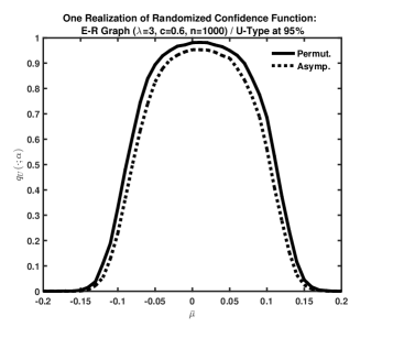
Figure 1. Illustration of a Randomized Confidence Interval at 95% When $\mu_{0}=0$ : The result is based on network Dependent observations on one realization of an Erdös-Rény random graph. See Section 3 for the meaning of the parameter values.

The randomized confidence function is not a familiar concept in econometrics. Instead, one may use a nonrandomized confidence set of the following form. Take $\beta\in(0,\alpha)$ and define for $\tau\in\{M,U\}$

(2.17) $$C_{\tau,\alpha}=\{\mu:q_{\tau}(\bar{\mu};\alpha-\beta)\geq 1-\alpha\}.$$

Then it is not hard to see from Corollary 2.1 that

$$\liminf_{n\rightarrow\infty}P\{\mu_{0}\in C_{\tau,\alpha}\}\geq 1-\alpha.$$

as $n\rightarrow\infty$. For example, we may take $\beta=0.005$, which is used in simulation studies in this paper. (In simulation studies unreported in this paper, the choice of $\beta=0$ was also used, and the results were not very different.)

3. Simulation Studies

3.1. Data Generating Process

This section presents and discusses a Monte Carlo simulation study which investigates the finite sample properties of the randomized subsampling approach in various situations with local dependence. As for local dependence, this study considered three kinds of data generating processes: (i) i.i.d. variables, (ii) variables having a dependency graph, (iii) network dependent variables. Both asymptotic and permutation critical values are considered.

As for the dependency graph case, we use two kinds of graphs. One is based on Erdös-Rényi graphs, and the other is based on Barabási-Albert graphs of preferential attachment. In an Erdös-Rényi random graph, each pair of the vertices form an edge with equal probability $p=\lambda/(n-1)$. The simulation study here chose $\lambda$ from $\{1,3,5\}$. Thus each vertex from this random graph has degree $\lambda$ on average, and the degree distribution is approximately a Poisson distribution with parameter $\lambda$ when the graph is large. For a Barabási-Albert random graph of preferential attachment, we first began with an Erdös-Rényi random graph of size $20$ with $\lambda=1$. Then we let the graph grow by adding each vertex sequentially and let the vertex form edges with $m$ other existing vertices. (We chose $m$ from $\{1,2,3\}$ for this study.) The probability of a new vertex forming an edge with an existing vertex is proportional to the number of the neighbors of the existing vertex. We keep adding new vertices until the size of the graph becomes $n$.

As for the generation of the random variables, we follow the design in Song (2015). We first generate $\{Y_{i}^{\ast}\}_{i=1}^{n}$ i.i.d. from $N(0,1)$. Let $E=\{e_{1},...,e_{S}\}$ be the set of edges in the graph with redundant edges removed from $E$ (i.e., remove $ji$ with $j<i$) and let $M$ be two-column matrix whose entries are of the form $[i_{s},j_{s}]$ for $e_{s}=i_{s}j_{s}$. Let $M$ be sorted on the first column so that $i_{s}\leq i_{s+1}$.

Step 1: For $s=1$, such that $e_{1}=i_{1}j_{1}$, we draw $Z_{1}\sim N(0,1)$ and set

$$(Y_{i_{1}},Y_{j_{1}})=\sqrt{1-c^{2}}\times(Y_{i_{1}}^{\ast},Y_{j_{1}}^{\ast})+c\times Z_{1},$$

where $c$ is a parameter that determines the strength of graph dependence. We replace $(Y_{i_{1}}^{\ast},Y_{j_{1}}^{\ast})$ by $(Y_{i_{1}},Y_{j_{1}})$, and redefine the series $\{Y_{i}^{\ast}\}_{i=1}^{n}$.

Step $s=2,...,S$: For $s>1$ such that $e_{s}=(i_{s},j_{s})$, we draw $Z_{s}\sim N(0,1)$ and set

$$(Y_{i_{s}},Y_{j_{s}})=\sqrt{1-c^{2}}\times(Y_{i_{s}}^{\ast},Y_{j_{s}}^{\ast})+c\times Z_{s}.$$

We replace $(Y_{i_{s}}^{\ast},Y_{j_{s}}^{\ast})$ by $(Y_{i_{s}},Y_{j_{s}})$, and redefine the series $\{Y_{i}^{\ast}\}_{i=1}^{n}$.

Turning now to the third data generation design involving network dependent observations, they are drawn from a jointly normal random vector with mean zero and a covariance matrix such that the correlation between two random variables at the distance $D$ is set to be $\exp(-\rho D)$, where $\rho$ is a parameter that determines the strength of the correlation. The parameter $\rho$ was taken from $\{1.0,1.5,2.0\}$. (Note that $\exp(-1)$ is roughly 0.3674 and $\exp(-2)$ is roughly 0.1353.) For the graph underlying the network-dependent observations, the simulation study considered a realization of a Erdös-Reényi random graph with $\lambda\in\{1,2\}$.

The size $n$ of the networks was taken from $\{500,1000,2000\}$. As for $R$ and $b_{n}$, we chose $R_{n}=\sqrt{n}$ and $b_{n}=n^{1/3}$ for the M-type statistic and $R_{n}=n$ and $b_{n}=n^{1/3}$ for the U-type statistic. The Monte Carlo simulation number and the permutation number (i.e., $L$) were set to be 1000, and the tuning parameter $\beta$ 0.005.

Table 1. The Empirical Coverage Probability of Confidence Interval: Independent Observations

U-Type Statistics

		Asymp.			Permut.
	$99\%$	$95\%$	$90\%$	$99\%$	$95\%$	$90\%$
$n=500$	0.968	0.919	0.875	0.990	0.946	0.895
$n=1000$	0.967	0.914	0.868	0.991	0.947	0.896
$n=2000$	0.963	0.909	0.861	0.991	0.945	0.894

M-Type Statistics

		Asymp.			Permut.
	$99\%$	$95\%$	$90\%$	$99\%$	$95\%$	$90\%$
$n=500$	0.980	0.928	0.874	0.986	0.931	0.876
$n=1000$	0.981	0.929	0.876	0.987	0.933	0.878
$n=2000$	0.980	0.928	0.875	0.987	0.933	0.878

Table 2. Empirical Coverage Probability: 95% for Dependency Graphs

U-Type Statistics

				E-R			B-A
			$\lambda=1$	$\lambda=3$	$\lambda=5$	$m=1$	$m=2$	$m=3$
		$n=500$	0.919	0.916	0.915	0.914	0.913	0.914
	$c=0.3$	$n=1000$	0.911	0.916	0.914	0.912	0.917	0.914
		$n=2000$	0.908	0.911	0.909	0.907	0.909	0.912
Asymp.
		$n=500$	0.917	0.919	0.919	0.916	0.917	0.916
	$c=0.6$	$n=1000$	0.916	0.912	0.910	0.917	0.915	0.914
		$n=2000$	0.910	0.913	0.912	0.908	0.913	0.911
		$n=500$	0.946	0.944	0.942	0.942	0.941	0.942
	$c=0.3$	$n=1000$	0.945	0.948	0.947	0.945	0.949	0.947
		$n=2000$	0.945	0.947	0.946	0.945	0.945	0.948
Permut.
		$n=500$	0.944	0.946	0.946	0.944	0.944	0.943
	$c=0.6$	$n=1000$	0.948	0.945	0.943	0.949	0.947	0.946
		$n=2000$	0.946	0.949	0.949	0.945	0.949	0.947

M-Type Statistics

				E-R			B-A
			$\lambda=1$	$\lambda=3$	$\lambda=5$	$m=1$	$m=2$	$m=3$
		$n=500$	0.928	0.926	0.925	0.923	0.923	0.924
	$c=0.3$	$n=1000$	0.926	0.930	0.929	0.926	0.930	0.929
		$n=2000$	0.927	0.929	0.927	0.926	0.928	0.930
Asymp.
		$n=500$	0.927	0.928	0.927	0.925	0.926	0.925
	$c=0.6$	$n=1000$	0.929	0.927	0.926	0.931	0.930	0.928
		$n=2000$	0.928	0.931	0.931	0.927	0.931	0.929
		$n=500$	0.932	0.929	0.929	0.927	0.927	0.927
	$c=0.3$	$n=1000$	0.930	0.934	0.932	0.930	0.934	0.932
		$n=2000$	0.931	0.933	0.931	0.931	0.932	0.935
Permut.
		$n=500$	0.930	0.931	0.930	0.928	0.929	0.928
	$c=0.6$	$n=1000$	0.933	0.931	0.930	0.934	0.933	0.932
		$n=2000$	0.932	0.935	0.935	0.932	0.935	0.933

Notes: The E-R represents Erdös-Rényi Random Graph with probability equal to $p=\lambda/(n-1)$, and $\lambda$ chosen from ${1,3,5}$, and the B-A represents Barabási-Albert random graph of preferential attachment, with $m$ refering to the number of links each new node forms with other existing nodes. A larger parameter $c$ represents a stronger correlation between two linked observations.

Table 3. Empirical Coverage Probability at 95% for Network Dependent Observations

U-Type Statistics

			Asymp.			Permut.
		$\rho=2.0$	$\rho=1.5$	$\rho=1.0$	$\rho=2.0$	$\rho=1.5$	$\rho=1.0$
	$n=500$	0.912	0.904	0.889	0.940	0.934	0.921
$\lambda=1$	$n=1000$	0.908	0.901	0.883	0.942	0.935	0.921
	$n=2000$	0.902	0.897	0.884	0.941	0.936	0.926
	$n=500$	0.900	0.881	0.817	0.930	0.914	0.854
$\lambda=2$	$n=1000$	0.904	0.877	0.811	0.939	0.914	0.857
	$n=2000$	0.893	0.873	0.805	0.934	0.918	0.857

M-Type Statistics

			Asymp.			Permut.
		$\rho=2.0$	$\rho=1.5$	$\rho=1.0$	$\rho=2.0$	$\rho=1.5$	$\rho=1.0$
	$n=500$	0.922	0.917	0.907	0.926	0.920	0.911
$\lambda=1$	$n=1000$	0.924	0.919	0.908	0.929	0.923	0.913
	$n=2000$	0.923	0.920	0.911	0.928	0.925	0.915
	$n=500$	0.915	0.902	0.860	0.918	0.906	0.865
$\lambda=2$	$n=1000$	0.921	0.904	0.862	0.925	0.909	0.867
	$n=2000$	0.917	0.904	0.862	0.921	0.909	0.869

Notes: The Erdös-Rényi Random Graph with probability equal to $p=\lambda/(n-1)$ was used. The correlation between linked observations is set to be $\exp(-\rho D)$ where $D$ represents the length of the shortest path between the two indices of the observations on the graph.

Table 4. Empirical False Coverage Probability at 95%

Independent Observations

			U-Type			M-Type
		$\bar{\mu}=0.06$	$\bar{\mu}=0.12$	$\bar{\mu}=0.18$	$\bar{\mu}=0.06$	$\bar{\mu}=0.12$	$\bar{\mu}=0.18$
	$n=500$	0.829	0.526	0.174	0.864	0.680	0.425
Asymp.	$n=1000$	0.745	0.244	0.015	0.815	0.506	0.190
	$n=2000$	0.554	0.032	0.000	0.716	0.257	0.030
	$n=500$	0.870	0.585	0.212	0.868	0.688	0.434
Permut.	$n=1000$	0.797	0.301	0.022	0.822	0.518	0.199
	$n=2000$	0.634	0.046	0.000	0.726	0.267	0.032

Dependency Graphs

			U-Type			M-Type
		$\bar{\mu}=0.06$	$\bar{\mu}=0.12$	$\bar{\mu}=0.18$	$\bar{\mu}=0.06$	$\bar{\mu}=0.12$	$\bar{\mu}=0.18$
	$n=500$	0.833	0.542	0.190	0.867	0.689	0.437
Asymp.	$n=1000$	0.744	0.248	0.014	0.819	0.513	0.194
	$n=2000$	0.558	0.032	0.000	0.719	0.260	0.030
	$n=500$	0.874	0.602	0.229	0.872	0.697	0.446
Permut.	$n=1000$	0.805	0.305	0.021	0.827	0.524	0.202
	$n=2000$	0.637	0.046	0.000	0.728	0.269	0.033

Notes: We chose $\lambda=3$ for the Erdös-Rényi (ER) Random Graph with $c=0.3$.

3.2. Results

3.2.1. Finite Sample Size Properties

First, let us report results on finite sample size properties. The results are shown in Tables 1 - 3. Table 1 presents the results from i.i.d. observations as a benchmark case. Table 2 uses simulated observations with dependency graphs where graphs are chosen to be from a single realization from two random graphs: Erdös-Reényi random graph and Barabási-Albert random graph. Finally, Table 3 shows the results from using network dependent observations.

First, for the U-type statistic approach, the permutation critical values perform conspicuously better than asymptotic critical values. Asymptotic critical values do not perform very well even in the case of independent observations. (See Table 1.) However, the contrast is much less stark for the M-type statistic approach.

Second, the U-type statistic approach exhibits more stable size properties than the M-type statistic approach. Interestingly, the performance does not seem to worsen much as the graph gets denser and the correlation stronger. This is perhaps because as one observation has more neighbors, the correlation between the observation and each neighbor tends to be weaker by the design of the data generating process.

Third, the randomized subsampling approach tends to over-reject the null hypothesis in the case of network dependence case (Table 3), where the overjection becomes severe as the correlation between linked observations gets stronger.

Throughout the simulation study, the increase in the sample size does not necessarily show better size properties. This may be because the graph tends to have more nodes with more neighbors as the sample size becomes larger, and this may offset the improvement in size properties partially.

3.2.2. Power Properties

Let us turn to the power properties of the randomized tests. The results are shown in Table 4. The false coverage probabilities using asymptotic critical values are lower than those using permutation critical values. This is not surprising given that the asymptotic critical values exhibit lower coverage probabilities at the true value of $\mu_{0}=0$ than permutation critical values.

Interestingly, the case of independent observations show only very slightly lower false coverage probabilities than the case of dependency graphs show similar results. This demonstrates the robustness properties of the randomized subsampling approach. However, in the case of network dependent observations, the false coverage probabilities are higher. The performance of randomized subsampling approach in the simulation designs and the choice of $R$, $b_{n}$, and $n$ does not seem stable for network dependent observations.

Finally, the M-type statistic approach exhibits larger false coverage probability than the U-type statistic approach, despite its worse size distortion. This may reflect the inferior performance of the M-type statistic approach as theoretically shown in terms of rate-dominance with size control.

4. Conclusion

This paper proposes a randomized subsampling approach to perform inference with locally dependent data when the dependence ordering is not known. This paper first introduces the notion of local dependence that does not invoke any reference to the underlying dependence ordering, and pursues ordering-free inference based on M-type statistic and U-type statistic approaches. The main results include establishing conditions for the local dependence which ensure the asymptotic validity of the approaches, and introducing the notion of rate dominance with size control to formally compare the two approaches, and show that U-type statistic approach rate-dominates the M-type statistic approach when permutation-based critical values are used. In general, there is a tradeoff between size and power in the randomized subsampling approach. Of course, when we have a huge number of observations, choosing $R_{n}$ and $b_{n}$ much smaller than $n$ can improve the small sample size property without hurting much its power. Some theoretical results suggesting a good combination of $R_{n}$ and $b_{n}$ in general would be desirable.

5. Appendix: Mathematical Proofs

Recall the definition of $Z_{i,n}=\Sigma_{n}^{-1/2}(X_{i,n}-\mu_{0})/\sqrt{d}$. We begin by providing a moment bound. The proof uses the recursive approach of a Doukhan-Portal type inequality (due to Doukhan and Portal (1983)) which is derived for our set-up. (See e.g. Lemma 3 of Andrews and Pollard (1994) and Lemma 14 of Doukhan and Louhichi (1999).)

Lemma 5.1.

Suppose that for some positive integer $q\geq 1$, and any positive sequence $a_{n}$, there exist $\bar{C}>0$ such that $b_{n}^{k}a_{n}^{-1}\lambda_{n}(k)\leq\bar{C}$, for all $n\geq 1$ and for each $2\leq k\leq 2q$.

Then there exists a constant $C_{d,q}>0$ that depends only on $d$, $q$ and $\bar{C}$ such that

$$\frac{1}{a_{n}|\Pi|}\sum_{\pi\in\Pi}\mathbf{E}\left(\left\|\frac{1}{\sqrt{b_{n}}}\sum_{i=1}^{b_{n}}Z_{\pi(i),n}\right\|^{2q}|\mathcal{C}_{n}\right)\leq C_{d,q}\sum_{k=1}^{2q}\max_{1\leq i\leq n}\mathbf{E}\left[\|Z_{i,n}\|^{2q}|\mathcal{C}_{n}\right],$$

for all $n\geq 1$.

The poof of Lemma 5.1 is found in Supplemental Note. Let us define

(5.1) $$\xi_{M,n}(\pi_{r}) \equiv \frac{1}{\sqrt{b_{n}}}\sum_{i=1}^{b_{n}}Z_{\pi_{r}(i),n},\text{ and }$$

(5.2) $$\xi_{U,n}(\pi_{r}) \equiv \frac{1}{b_{n}}\sum_{i=1}^{b_{n}}\sum_{j=1,i\neq j}^{b_{n}}Z_{\pi_{r}(i),n}^{\prime}Z_{\pi_{r}(j),n},$$

and let for each $\tau\in\{M,U\}$,

$$S_{\tau,n}^{*}(\boldsymbol{\pi}) \equiv \frac{1}{\sqrt{R_{n}}}\sum_{r=1}^{R_{n}}\xi_{\tau,n}(\pi_{r}).$$

We focus on the asymptotic properties of $S_{\tau,n}^{*}(\boldsymbol{\pi})$. For this, write (with $\tau\in\{M,U\}$)

(5.3) $$S_{\tau,n}^{*}(\boldsymbol{\pi})=S_{\tau,A,n}^{*}(\boldsymbol{\pi})+S_{\tau,B,n}^{*}(\boldsymbol{\pi}),$$

where

$$S_{\tau,A,n}^{*}(\boldsymbol{\pi}) = \frac{1}{\sqrt{R_{n}}}\sum_{r=1}^{R_{n}}\left(\xi_{\tau,n}(\pi_{r})-\mathbf{E}[\xi_{\tau,n}(\pi_{r})|\mathscr{Z}_{n}]\right)\textnormal{ and }$$

$$S_{\tau,B,n}^{*}(\boldsymbol{\pi}) = \frac{1}{\sqrt{R_{n}}}\sum_{r=1}^{R_{n}}\mathbf{E}[\xi_{\tau,n}(\pi_{r})|\mathscr{Z}_{n}].$$

The following lemma gives the convergence rates of $S_{\tau,B,n}^{*}(\boldsymbol{\pi})$ for each $\tau\in\{M,U\}$.

Lemma 5.2.

Suppose that Assumption 2.3 holds. Then

$$\mathbf{E}[||S_{M,B,n}^{*}(\boldsymbol{\pi})||^{2}] = O(R_{n}b_{n}(\bar{\lambda}_{n}(2)+n^{-1})),\text{ and }$$

$$\mathbf{E}[(S_{U,B,n}^{*}(\boldsymbol{\pi}))^{2}] = O(R_{n}b_{n}^{2}\{\bar{\lambda}_{n}(4)+n^{-1}(\bar{\lambda}_{n}(2)+\bar{\lambda}_{n}(3))+n^{-2}\}).$$

Proof: For notational brevity, denote

(5.4) $$\zeta_{i,j,n}\equiv Z_{i,n}^{\prime}Z_{j,n},\textnormal{ and }\tilde{\zeta}_{i,j,n}\equiv Z_{i,n}Z_{j,n}^{\prime}.$$

Since we draw $\pi_{r}$’s i.i.d. from the uniform distribution on $\Pi$, we can rewrite

$$S_{M,B,n}^{*}(\boldsymbol{\pi})=\frac{\sqrt{R_{n}b_{n}}}{n}\sum_{i=1}^{n}Z_{i,n}.$$

Hence for some constant $C>0$,

$$\mathbf{E}[||S_{M,B,n}^{*}(\boldsymbol{\pi})||^{2}] = \frac{R_{n}b_{n}}{n^{2}}\sum_{i=1}^{n}\mathbf{E}[\zeta_{i,i,n}]+\frac{R_{n}b_{n}}{n^{2}}\sum_{i=1}^{n}\sum_{j=1:j\neq i}^{n}\mathbf{E}[\zeta_{i,j,n}]$$

$$\leq \frac{R_{n}b_{n}}{n^{2}}\sum_{i=1}^{n}\mathbf{E}[\zeta_{i,i,n}]+CR_{n}b_{n}\lambda_{n}(2)=O(R_{n}b_{n}(n^{-1}+\lambda_{n}(2))).$$

Let us now turn to the second statement. We write

$$S_{U,B,n}^{*}(\boldsymbol{\pi})=\frac{\sqrt{R_{n}}(b_{n}-1)}{n(n-1)}\sum_{i=1}^{n}\sum_{j=1:j\neq i}^{n}\zeta_{i,j,n}.$$

Note that

$$\mathbf{E}[(S_{U,B,n}^{*}(\boldsymbol{\pi}))^{2}] = R_{n}(b_{n}-1)^{2}\mathbf{E}\left[\frac{1}{n^{2}(n-1)^{2}}\sum_{i=1}^{n}\sum_{j=1:j\neq i}^{n}\zeta_{i,j,n}^{2}\right]+R_{n}(b_{n}-1)^{2}A_{n},$$

where

(5.5) $$A_{n}=\frac{1}{n^{2}(n-1)^{2}}\sum_{(i_{1},j_{1},i_{2},j_{2})}\mathbf{E}\left[\zeta_{i_{1},j_{1},n}\zeta_{i_{2},j_{2},n}\right],$$

and the sum over $(i_{1},j_{1},i_{2},j_{2})$ includes 4-tuples of positive integers from $1$ to $n$ such that $i_{1}\neq j_{1}$, $i_{2}\neq j_{2}$, and $(i_{1},j_{1})\neq(i_{2},j_{2})$. The leading term in the decomposition above is $O(n^{-2}R_{n}b_{n}^{2})$ by the moment conditions in Assumption 2.3.

Let us analyze $A_{n}$ which we write

$$A_{n}=4B_{1,n}+B_{2,n},$$

where

$$B_{1,n} = \frac{1}{n^{2}(n-1)^{2}}\sum_{(i_{1},j_{1},j_{2})^{*}}\mathbf{E}\left[\zeta_{i_{1},j_{1},n}\zeta_{i_{1},j_{2},n}\right],\textnormal{ and }$$

$$B_{2,n} = \frac{1}{n^{2}(n-1)^{2}}\sum_{(i_{1},j_{1},i_{2},j_{2})^{*}}\mathbf{E}\left[\zeta_{i_{1},j_{1},n}\zeta_{i_{2},j_{2},n}\right],$$

where the sum over $(i_{1},j_{1},j_{2})^{*}$ is over all 3-tuples of distinct integers in $\{1,...,n\}$ and the sum over $(i_{1},j_{1},i_{2},j_{2})^{*}$ is over all 4-tuples of distinct integers in $\{1,...,n\}$. The factor 4 in front of $B_{1,n}$ appears because for each 4-tuple, say $(i_{1}^{\prime},j_{1}^{\prime},i_{2}^{\prime},j_{2}^{\prime})$, there are four ways to form a pair with one from $(i_{1}^{\prime},j_{1}^{\prime})$ and the other from $(i_{2}^{\prime},j_{2}^{\prime})$.

We write

$$\quad\quad B_{1,n} = \frac{1}{n^{2}(n-1)^{2}}\sum_{(i_{1},j_{1},j_{2})^{*}}\textnormal{tr}\left(\mathbf{E}[\tilde{\zeta}_{i_{1},i_{1},n}\tilde{\zeta}_{j_{2},j_{1},n}]-\mathbf{E}[\mathbf{E}[\tilde{\zeta}_{i_{1},i_{1},n}|\mathcal{C}_{n}]\mathbf{E}[\tilde{\zeta}_{j_{2},j_{1},n}|\mathcal{C}_{n}]]\right)$$

$$+\frac{1}{n^{2}(n-1)^{2}}\sum_{(i_{1},j_{1},j_{2})^{*}}\mathbf{E}\left[\textnormal{tr}\left(\mathbf{E}[\tilde{\zeta}_{i_{1},i_{1},n}|\mathcal{C}_{n}]\mathbf{E}[\tilde{\zeta}_{j_{2},j_{1},n}|\mathcal{C}_{n}]\right)\right].$$

By Assumption 2.3(i), the last term is bounded by $Cn^{-1}\mathbf{E}[\lambda_{n}(2)]=Cn^{-1}\bar{\lambda}_{n}(2)$, for some constant $C>0$ that does not depend on $n$.

We turn to the leading term on the right hand side of (5). Note that

$$\mathcal{P}(\{i_{1},j_{1},j_{2}\})=\{\{\{i_{1}\},\{j_{1},j_{2}\}\},\{\{i_{1},j_{1}\},\{j_{2}\}\},\{\{i_{1},j_{2}\},\{j_{1}\}\}\}.$$

The trace in the leading sum in (5) is bounded by $d\mathbf{E}[c_{n}(\{i_{1}\},\{j_{1},j_{2}\})]$. As we can also write (using the fact that $\mathbf{E}\left[Z_{j_{1},n}|\mathcal{C}_{n}\right]=0$)

$$\mathbf{E}[\tilde{\zeta}_{i_{1},i_{1},n}\tilde{\zeta}_{j_{2},j_{1},n}|\mathcal{C}_{n}]=\mathbf{E}[\tilde{\zeta}_{i_{1},i_{1},n}\tilde{\zeta}_{j_{2},j_{1},n}|\mathcal{C}_{n}]-\mathbf{E}[Z_{i_{1},n}Z_{i_{1},n}^{\prime}Z_{j_{2},n}|\mathcal{C}_{n}]\mathbf{E}[Z_{j_{1},n}^{\prime}|\mathcal{C}_{n}],$$

the trace in the leading sum of (5) is bounded by

$$d\mathbf{E}[c_{n}(\{i_{1},j_{2}\},\{j_{1}\})]+dC\mathbf{E}[c_{n}(\{j_{2}\},\{j_{1}\})],$$

for some constant $C>0$, where $c_{n}(\{j_{2}\},\{j_{1}\})$ is due to $\mathbf{E}[\tilde{\zeta}_{j_{2},j_{1},n}|\mathcal{C}_{n}]$. Similarly, the same trace is also bounded by $d\mathbf{E}[c_{n}(\{i_{1},j_{1}\},\{j_{2}\})]+dC\mathbf{E}[c_{n}(\{j_{2}\},\{j_{1}\})]$. Therefore, the leading sum on the right hand side of (5) is bounded by $Cn^{-1}(\mathbf{E}[\lambda_{n}(3)]+\mathbf{E}[\lambda_{n}(2)])=Cn^{-1}(\bar{\lambda}_{n}(2)+\bar{\lambda}_{n}(3))$, so that

$$B_{1,n}\leq Cn^{-1}(\bar{\lambda}_{n}(2)+\bar{\lambda}_{n}(3)).$$

Let us turn to $B_{2,n}$. By the definition of $\lambda_{n}(\cdot)$, we have

$$B_{2,n}\leq C\mathbf{E}[\lambda_{n}(4)]=C\bar{\lambda}_{n}(4),$$

for some $C>0$. We conclude that

$$R_{n}(b_{n}-1)^{2}A_{n}=O(R_{n}b_{n}^{2}\{\bar{\lambda}_{n}(4)+n^{-1}(\bar{\lambda}_{n}(3)+\bar{\lambda}_{n}(2))\}),$$

completing the proof. $\blacksquare$

Lemma 5.3.

(i) Under Assumptions 2.1 M-(i) and 2.3, $Var(S_{M,A,n}^{*}(\boldsymbol{\pi})|\mathscr{Z}_{n})=I_{d}/d+o_{P}(1)$.

(ii) Under Assumptions 2.2 U-(i) and 2.3, $Var(S_{U,A,n}^{*}(\boldsymbol{\pi})|\mathscr{Z}_{n})=1+o_{P}(1).$

Proof: (i) Write

$$Var(S_{M,A,n}^{*}(\boldsymbol{\pi})|\mathscr{Z}_{n})=\frac{1}{n}\sum_{i=1}^{n}Z_{i,n}Z_{i,n}^{\prime}-\overline{Z}_{n}\overline{Z}_{n}^{\prime}.$$

As for the leading term,

$$\mathbf{E}\left(\left\|\frac{1}{n}\sum_{i=1}^{n}\left(Z_{i,n}Z_{i,n}^{\prime}-\mathbf{E}[Z_{i,n}Z_{i,n}^{\prime}|\mathcal{C}_{n}]\right)\right\|^{2}\right)$$

$$= \frac{1}{n^{2}}\sum_{i=1}^{n}\textnormal{tr}\left(\mathbf{E}\left[(Z_{i,n}Z_{i,n}^{\prime}-\mathbf{E}[Z_{i,n}Z_{i,n}^{\prime}|\mathcal{C}_{n}])^{2}\right]\right)$$

$$+ \frac{1}{n^{2}}\sum_{i=1}^{n}\sum_{j=1,j\neq i}^{n}\textnormal{tr}\left(\mathbf{E}\left[(Z_{i,n}Z_{i,n}^{\prime}-\mathbf{E}[Z_{i,n}Z_{i,n}^{\prime}|\mathcal{C}_{n}])(Z_{j,n}Z_{j,n}^{\prime}-\mathbf{E}[Z_{j,n}Z_{j,n}^{\prime}|\mathcal{C}_{n}])^{\prime}\right]\right).$$

The right hand side of the above equality is equal to $O(n^{-1}+\lambda_{n}(2))$. In the same way,

(5.8) $$\overline{Z}_{n}=\frac{1}{n}\sum_{i=1}^{n}Z_{i,n}=O_{P}(n^{-1/2}+\sqrt{\lambda_{n}(2)}).$$

Therefore, $\overline{Z}_{n}\overline{Z}_{n}^{\prime}=o_{P}(1)$, and

$$Var(S_{M,A,n}^{*}(\boldsymbol{\pi})|\mathscr{Z}_{n})=\frac{1}{n}\sum_{i=1}^{n}\mathbf{E}[Z_{i,n}Z_{i,n}^{\prime}|\mathcal{C}_{n}]+o_{P}(1)=I_{d}+o_{P}(1).$$

(ii) Let us consider

$$Var(S_{U,A,n}^{*}(\boldsymbol{\pi})|\mathscr{Z}_{n}) = \frac{1}{n(n-1)}\sum_{i=1}^{n}\sum_{j=1:j\neq i}^{n}\zeta_{i,j,n}^{2}-\left(\frac{1}{n(n-1)}\sum_{i=1}^{n}\sum_{j=1:j\neq i}^{n}\zeta_{i,j,n}\right)^{2}$$

$$= \frac{1}{n(n-1)}\sum_{i=1}^{n}\sum_{j=1:j\neq i}^{n}\zeta_{i,j,n}^{2}+o_{P}(1),$$

because, as we saw in the proof of Lemma 5.2,

$$\frac{1}{n(n-1)}\sum_{i=1}^{n}\sum_{j=1:j\neq i}^{n}\zeta_{i,j,n}=o_{P}(1).$$

Now we write

(5.9) $$\frac{1}{n(n-1)}\sum_{i=1}^{n}\sum_{j=1:j\neq i}^{n}\zeta_{i,j,n}^{2}=\frac{1}{n(n-1)}\sum_{i=1}^{n}\sum_{j=1:j\neq i}^{n}\mathbf{E}[\zeta_{i,j,n}^{2}|\mathcal{C}_{n}]+\Delta_{n},$$

where

$$\Delta_{n}=\frac{1}{n(n-1)}\sum_{i=1}^{n}\sum_{j=1:j\neq i}^{n}\left(\zeta_{i,j,n}^{2}-\mathbf{E}[\zeta_{i,j,n}^{2}|\mathcal{C}_{n}]\right).$$

Rewrite the leading term on the right hand side of (5.9) as

$$1+\frac{1}{n(n-1)}\sum_{i=1}^{n}\sum_{j=1:j\neq i}^{n}\textnormal{tr}\left(\mathbf{E}[(Z_{i,n}Z_{i,n}^{\prime}-I_{d})(Z_{j,n}Z_{j,n}^{\prime}-I_{d})|\mathcal{C}_{n}]\right).$$

The last term is bouned by $C\lambda_{n}(2)=o_{P}(1)$.

We turn to $\Delta_{n}$. Write

$$\mathbf{E}[\Delta_{n}^{2}] = \frac{1}{n^{2}(n-1)^{2}}\sum_{(i_{1},j_{1},i_{2},j_{2})}\mathbf{E}\left[\zeta_{i_{1},j_{1},n}^{2}\zeta_{i_{2},j_{2},n}^{2}\right]$$

$$- \frac{1}{n^{2}(n-1)^{2}}\sum_{(i_{1},j_{1},i_{2},j_{2})}\mathbf{E}\left[\mathbf{E}[\zeta_{i_{1},j_{1},n}^{2}|\mathcal{C}_{n}]\mathbf{E}[\zeta_{i_{2},j_{2},n}^{2}|\mathcal{C}_{n}]\right],$$

where the sum over $(i_{1},j_{1},i_{2},j_{2})$ is over all the 4-tuples of positive integers from $\{1,...,n\}$ such that 4-tuples of positive integers from $1$ to $n$ such that $i_{1}\neq j_{1}$, $i_{2}\neq j_{2}$, and $(i_{1},j_{1})\neq(i_{2},j_{2})$. Again, we write

$$\mathbf{E}[\Delta_{n}^{2}]=\Delta_{1,n}+\Delta_{2,n},$$

where

$$\Delta_{1,n} = \frac{1}{n^{2}(n-1)^{2}}\sum_{(i_{1},j_{1},j_{2})^{*}}\mathbf{E}\left[\zeta_{i_{1},j_{1},n}^{2}\zeta_{i_{1},j_{2},n}^{2}\right]$$

$$- \frac{1}{n^{2}(n-1)^{2}}\sum_{(i_{1},j_{1},j_{2})^{*}}\mathbf{E}\left[\mathbf{E}[\zeta_{i_{1},j_{1},n}^{2}|\mathcal{C}_{n}]\mathbf{E}[\zeta_{i_{1},j_{2},n}^{2}|\mathcal{C}_{n}]\right]$$

and

$$\Delta_{2,n} = \frac{1}{n^{2}(n-1)^{2}}\sum_{(i_{1},j_{1},i_{1},j_{2})^{*}}\mathbf{E}\left[\zeta_{i_{1},j_{1},n}^{2}\zeta_{i_{2},j_{2},n}^{2}\right]$$

$$- \frac{1}{n^{2}(n-1)^{2}}\sum_{(i_{1},j_{1},i_{2},j_{2})^{*}}\mathbf{E}\left[\mathbf{E}[\zeta_{i_{1},j_{1},n}^{2}|\mathcal{C}_{n}]\mathbf{E}[\zeta_{i_{2},j_{2},n}^{2}|\mathcal{C}_{n}]\right].$$

As in the proof of Lemma 5.2, the sum over $(i_{1},j_{1},j_{2})^{*}$ is over all 3-tuples of distinct integers in $\{1,...,n\}$ and the sum over $(i_{1},j_{1},i_{2},j_{2})^{*}$ is over all 4-tuples of distinct integers in $\{1,...,n\}$. By Assumption 2.3, and by counting the number of all 3-tuples of distinct integers in $\{1,...,n\}$, we have

$$\Delta_{1,n}=O(n^{-1}).$$

As for $\Delta_{2,n}$, we write

$$\Delta_{2,n}=\frac{1}{n^{2}(n-1)^{2}}\sum_{(i_{1},j_{1},i_{1},j_{2})^{*}}\mathbf{E}\left[Cov(\zeta_{i_{1},j_{1},n}^{2},\zeta_{i_{2},j_{2},n}^{2}|\mathcal{C}_{n})\right]\leq C\mathbf{E}[\lambda_{n}(4)]=o(1).$$

We conclude that $\Delta_{n}=o_{P}(1).$ $\blacksquare$

Recall the definitions of $\xi_{M,n}(\pi_{r})$ and $\xi_{U,n}(\pi_{r})$ in (5.1).

Lemma 5.4.

Suppose that the conditions of Lemma 5.1 hold. Then for any $a\in\mathbf{R}^{d}$,

$$\mathbf{E}\left[|a^{\prime}\xi_{M,n}(\pi_{r})-\mathbf{E}[a^{\prime}\xi_{M,n}(\pi_{r})|\mathscr{Z}_{n}]|^{3}\right] = O(1),\text{ and }$$

$$\mathbf{E}\left[|\xi_{U,n}(\pi_{r})-\mathbf{E}[\xi_{U,n}(\pi_{r})|\mathscr{Z}_{n}]|^{3}\right] = O(1).$$

Proof: We bound for some $C>0$,

$$\mathbf{E}[|a^{\prime}\xi_{M,n}(\pi_{r})-\mathbf{E}[a^{\prime}\xi_{M,n}(\pi_{r})|\mathscr{Z}_{n}]|^{3}]\leq C\mathbf{E}\left[\left(\mathbf{E}[|a^{\prime}\xi_{M,n}(\pi_{r})|^{4}|\mathscr{Z}_{n}]\right)^{3/4}\right]\leq C\left(\mathbf{E}[|a^{\prime}\xi_{M,n}(\pi_{r})|^{4}]\right)^{3/4}.$$

Note that

$$\mathbf{E}[|a^{\prime}\xi_{M,n}(\pi_{r})|^{4}] \leq \frac{1}{|\Pi|}\sum_{\pi\in\Pi}\mathbf{E}\left[\frac{1}{\sqrt{b_{n}}}\sum_{i=1}^{b_{n}}a^{\prime}Z_{\pi(i),n}\right]^{4}\leq C,$$

for some $C>0$ by Lemma 5.1.

As for the second statement, similarly as before, we bound for some $C>0$,

$$\mathbf{E}[|\xi_{U,n}(\pi_{r})-\mathbf{E}[\xi_{U,n}(\pi_{r})|\mathscr{Z}_{n}]|^{3}]\leq C\left(\mathbf{E}[\xi_{U,n}(\pi_{r})^{4}]\right)^{3/4}.$$

Note that

$$\mathbf{E}[\xi_{U,n}(\pi_{r})^{4}] \leq \frac{1}{|\Pi|}\sum_{\pi\in\Pi}\mathbf{E}\left[\frac{1}{b_{n}}\sum_{i=1}^{b_{n}}\sum_{j=1,i\neq j}^{b_{n}}\zeta_{\pi(i),\pi(j),n}\right]^{4}.$$

We bound the last term by

$$\frac{2^{3}}{|\Pi|}\sum_{\pi\in\Pi}\mathbf{E}\left(\left(\frac{1}{\sqrt{b_{n}}}\sum_{i=1}^{b_{n}}Z_{\pi(i),n}\right)^{\prime}\left(\frac{1}{\sqrt{b_{n}}}\sum_{i=1}^{b_{n}}Z_{\pi(i),n}\right)\right)^{4}$$

$$+ \frac{2^{3}}{|\Pi|}\sum_{\pi\in\Pi}\mathbf{E}\left(\frac{1}{b_{n}}\sum_{i=1}^{b_{n}}Z_{\pi(i),n}^{\prime}Z_{\pi(i),n}\right)^{4}\equiv D_{1,n}+D_{2,n}.$$

By Lemma 5.1, we have for some $C>0$, $D_{1,n}\leq C$. As for $D_{2,n}$, we use Jensen’s inequality and bound

$$D_{2,n}\leq\frac{2^{3}}{|\Pi|}\sum_{\pi\in\Pi}\frac{1}{b_{n}}\sum_{i=1}^{b_{n}}\mathbf{E}\left[Z_{\pi(i),n}^{\prime}Z_{\pi(i),n}\right]^{4}\leq C,$$

for some $C>0$, completing the proof. $\blacksquare$

Lemma 5.5.

Suppose that Assumption 2.3 holds, and that $\lambda_{n}(2)=o_{P}(1)$ as $n\rightarrow\infty$. Then

(5.10) $$\frac{1}{n}\sum_{i=1}^{n}(X_{i,n}-\overline{X}_{n})(X_{i,n}-\overline{X}_{n})^{\prime}=\Sigma_{n}+O_{P}(n^{-1/2}+\sqrt{\lambda_{n}(2)}).$$

Proof: Let $D_{n}=\frac{1}{n}\sum_{i=1}^{n}\left(Z_{i,n}Z_{i,n}^{\prime}-\mathbf{E}[Z_{i,n}Z_{i,n}^{\prime}|\mathcal{C}_{n}]\right)-\overline{Z}_{n}\overline{Z}_{n}^{\prime}$ and write

$$\frac{1}{n}\sum_{i=1}^{n}(X_{i,n}-\overline{X}_{n})(X_{i,n}-\overline{X}_{n})^{\prime}=\Sigma_{n}+\Sigma_{n}^{1/2}D_{n}\Sigma_{n}^{1/2}.$$

The desired result follows because $D_{n}=O_{P}(n^{-1/2}+\sqrt{\lambda_{n}(2)})$. $\blacksquare$

Lemma 5.6.

Suppose that Assumption 2.3 holds. Then

$$Var\left(\frac{1}{\sqrt{R_{n}}}\sum_{r=1}^{R_{n}}\frac{1}{\sqrt{b_{n}}}\sum_{i=1}^{b_{n}}Z_{\pi_{r}(i),n}|\mathscr{Z}_{n}\right)=I_{d}/d+o_{P}(1).$$

Proof: We write

$$Var\left(\frac{1}{\sqrt{R_{n}}}\sum_{r=1}^{R_{n}}\frac{1}{\sqrt{b_{n}}}\sum_{i=1}^{b_{n}}Z_{\pi_{r}(i),n}|\mathscr{Z}_{n}\right)$$

$$= \frac{1}{R_{n}}\sum_{r=1}^{R_{n}}\mathbf{E}\left[\left(\frac{1}{\sqrt{b_{n}}}\sum_{i=1}^{b_{n}}(Z_{\pi_{r}(i),n}-\overline{Z}_{n})\right)\left(\frac{1}{\sqrt{b_{n}}}\sum_{i=1}^{b_{n}}(Z_{\pi_{r}(i),n}-\overline{Z}_{n})\right)^{\prime}|\mathscr{Z}_{n}\right].$$

We write the last term as $E_{1,n}+E_{2,n}$, where

$$E_{1,n} = \frac{1}{R_{n}}\sum_{r=1}^{R_{n}}\mathbf{E}\left[\frac{1}{b_{n}}\sum_{i=1}^{b_{n}}(Z_{\pi_{r}(i),n}-\overline{Z}_{n})(Z_{\pi_{r}(i),n}-\overline{Z}_{n})^{\prime}|\mathscr{Z}_{n}\right]\textnormal{ and }$$

$$E_{2,n} = \frac{1}{R_{n}}\sum_{r=1}^{R_{n}}\mathbf{E}\left[\frac{1}{b_{n}}\sum_{i,j=1,i\neq j}^{b_{n}}(Z_{\pi_{r}(i),n}-\overline{Z}_{n})(Z_{\pi_{r}(j),n}-\overline{Z}_{n})^{\prime}|\mathscr{Z}_{n}\right].$$

As for the first term, we write

$$E_{1,n} = \frac{1}{n}\sum_{i=1}^{n}Z_{i,n}Z_{i,n}^{\prime}-\overline{Z}_{n}\overline{Z}_{n}^{\prime}$$

$$= \frac{1}{n}\sum_{i=1}^{n}\left(Z_{i,n}Z_{i,n}^{\prime}-\mathbf{E}[Z_{i,n}Z_{i,n}^{\prime}]\right)-\overline{Z}_{n}\overline{Z}_{n}^{\prime}+\frac{1}{n}\sum_{i=1}^{n}\mathbf{E}[Z_{i,n}Z_{i,n}^{\prime}].$$

The last term is $I_{d}$ and by (5.8),

(5.11) $$\overline{Z}_{n}\overline{Z}_{n}^{\prime}=O_{P}(n^{-1}+\lambda_{n}(2)).$$

As for the leading term,

$$\mathbf{E}\left\|\frac{1}{n}\sum_{i=1}^{n}\left(Z_{i,n}Z_{i,n}^{\prime}-\frac{1}{d}I_{d}\right)\right\|^{2}$$

$$= \frac{1}{n^{2}}\sum_{i,j=1,i\neq j}^{n}\textnormal{tr}\left(\mathbf{E}\left[\left(Z_{i,n}Z_{i,n}^{\prime}-\frac{1}{d}I_{d}\right)\left(Z_{j,n}Z_{j,n}^{\prime}-\frac{1}{d}I_{d}\right)^{\prime}\right]\right)+O(n^{-1}).$$

The leading term is bounded by $C\mathbf{E}[\lambda_{n}(2)]=C\bar{\lambda}_{n}(2)$. Hence

$$E_{1,n}=\frac{1}{d}I_{d}+O_{P}(n^{-1/2}+\sqrt{\lambda_{n}(2)}).$$

Let us turn to $E_{2,n}$ which we write as

$$\frac{b_{n}-1}{n(n-1)}\sum_{i,j=1,i\neq j}^{n}\left(Z_{i,n}Z_{j,n}^{\prime}-\mathbf{E}[Z_{i,n}Z_{j,n}^{\prime}]\right)$$

$$+ \frac{b_{n}-1}{n(n-1)}\sum_{i,j=1,i\neq j}^{n}\mathbf{E}[Z_{i,n}Z_{j,n}^{\prime}]+(b_{n}-1)B_{n},$$

where

$$B_{n} = \overline{Z}_{n}\overline{Z}_{n}^{\prime}-\frac{1}{n(n-1)}\sum_{i,j=1,i\neq j}^{n}\overline{Z}_{n}Z_{j,n}^{\prime}-\frac{1}{n(n-1)}\sum_{i,j=1,i\neq j}^{n}Z_{i,n}\overline{Z}_{n}^{\prime}$$

$$= O_{P}(n^{-1}+\lambda_{n}(2)),$$

using the same argument as in (5.11).

The second term in (5) is bounded by $b_{n}\lambda_{n}(2)$. As for the leading term in (5), we can follow the same arguments in the proof of Lemma 5.2 and show that it is equal to $o_{P}(1)$. Therefore, $E_{2,n}=o_{P}(1)$. $\blacksquare$

Proof of Theorem 2.1: (i) Let us consider the first statement. Recall the definition of $S_{M,A,n}^{*}(\boldsymbol{\pi})$ prior to Lemma 5.2. By Lemma 5.3, we find that

$$\mathbf{E}\left[|S_{M,A,n}^{*}(\boldsymbol{\pi})||\mathscr{Z}_{n}\right]=O_{P}(1).$$

Combining this with (5.10) and using (5.3) and Lemma 5.2, we obtain that

$${S}_{M,n}(\mu_{0};\boldsymbol{\pi})=S_{M,A,n}^{*}(\boldsymbol{\pi})+o_{P}(1).$$

We focus on $S_{M,A,n}^{*}(\boldsymbol{\pi})$. Since $\{\xi_{M,n}(\pi_{r})\}_{r=1}^{R_{n}}$ is a triangular array that is rowwise i.i.d. conditional on $\mathscr{Z}_{n}$, we deduce that by Berry-Esseen lemma (e.g. Theorem 3 of Chow and Teicher (1988), p.304), for some $C>0$,

$$\left|P\left\{\frac{S_{M,A,n}^{*}(\boldsymbol{\pi})}{\sigma_{M,n}(\mathscr{Z}_{n})}\leq t|\mathscr{Z}_{n}\right\}-\Phi(t)\right|\leq\frac{C}{R_{n}^{3/2}}\sum_{r=1}^{R_{n}}\mathbf{E}[|\xi_{M,n}(\pi_{r})-\mathbf{E}[\xi_{M,n}(\pi_{r})|\mathscr{Z}_{n}]|^{3}|\mathscr{Z}_{n}],$$

where $\sigma_{M,n}^{2}(\mathscr{Z}_{n})=Var(S_{M,A,n}^{*}(\boldsymbol{\pi})|\mathscr{Z}_{n})$. By Lemma 5.4, the expected value of the last bound has a rate $O(R_{n}^{-1/2})$. In view of Lemma 5.5, this completes the proof of the first statement.

Let us turn to the second statement. From (2.4.2), we write

$$S_{M,n}(\overline{X}_{n};\boldsymbol{\pi})=\frac{1}{R_{n}b_{n}}\sum_{r_{1}=1}^{R_{n}}\sum_{r_{2}=1}^{R_{n}}\sum_{i_{1}=1}^{b_{n}}\sum_{i_{2}=1}^{b_{n}}Z_{\pi_{r_{1}}(i_{1}),n}^{\prime}Z_{\pi_{r_{2}}(i_{2}),n}+B_{M,n}+o_{P}(1),$$

where $o_{P}(1)$ is due to the estimation error in $\hat{\Sigma}$, and $B_{M,n}$ is as defined in (2.7). By Lemma 5.6 and in view of the heuristics in Section 2.4.2, we find that

$$B_{M,n}=O_{P}\left(R_{n}b_{n}(n^{-1/2}+n\lambda_{n}(2))^{2}+\sqrt{R_{n}b_{n}/n}\right)=o_{P}(1).$$

Therefore,

$$S_{M,n}(\overline{X}_{n};\boldsymbol{\pi})=\tilde{S}_{M,n}(\mu_{0};\boldsymbol{\pi})+o_{P}(1),$$

where $\tilde{S}_{M,n}(\mu_{0};\boldsymbol{\pi})$ is the same as $S_{M,n}(\mu_{0};\boldsymbol{\pi})$ except that $\hat{\Sigma}$ is replaced by $\Sigma_{n}$.

Hence the conditional distribution of $S_{M,n}(\overline{X}_{n};\boldsymbol{\pi})$ given $\mathscr{Z}_{n}$ is the same as that of $S_{M,n}(\mu_{0};\boldsymbol{\pi})$ up to a $o_{P}(1)$ term. From the proof of the first statement, we find that the conditional CDF of $S_{M,n}(\mu_{0};\boldsymbol{\pi})$ given $\mathscr{Z}_{n}$ converges (uniformly over the evaluation points) in probability to $G_{0}$, which completes the proof.

(ii) The proof is almost the same as that of (i). $\blacksquare$

Proof of Theorem 2.2: (i) Write $S_{M,n}(\bar{\mu};\boldsymbol{\pi})=(A_{M,n}+\delta)^{\prime}\hat{\Sigma}^{-1}(A_{M,n}+\delta)$, where

$$A_{M,n}=\frac{1}{\sqrt{dR_{n}b_{n}}}\sum_{r=1}^{R_{n}}\sum_{i=1}^{b_{n}}(X_{\pi_{r}(i)}-\mu_{\delta,M}).$$

Note that

$$A_{M,n}=\frac{1}{\sqrt{dR_{n}b_{n}}}\sum_{r=1}^{R_{n}}\sum_{i=1}^{b_{n}}(X_{\pi_{r}(i)}-\overline{X}_{n})+O_{P}\left(\frac{\sqrt{R_{n}b_{n}}}{\sqrt{n}}\right).$$

The last $O_{P}$ term is $o_{P}(1)$ by Assumption 2.1 M-(i). Thus we obtain the desired result from the proof of Theorem 2.1 and the continuous mapping theorem.

(ii) We write $S_{U,n}(\bar{\mu};\boldsymbol{\pi})=S_{U,n}(\mu_{\delta,U};\boldsymbol{\pi})+D_{U,n}$, where

$$D_{U,n} = \frac{1}{\sqrt{R_{n}}}\sum_{r=1}^{R_{n}}\frac{1}{db_{n}}\sum_{i=1}^{b_{n}}\sum_{j=1:j\neq i}^{b_{n}}(X_{\pi_{r}(i)}-\bar{\mu})^{\prime}\hat{\Sigma}^{-1}(X_{\pi_{r}(j)}-\bar{\mu})$$

$$- \frac{1}{\sqrt{R_{n}}}\sum_{r=1}^{R_{n}}\frac{1}{db_{n}}\sum_{i=1}^{b_{n}}\sum_{j=1:j\neq i}^{b_{n}}(X_{\pi_{r}(i)}-\mu_{\delta,U})^{\prime}\hat{\Sigma}^{-1}(X_{\pi_{r}(j)}-\mu_{\delta,U}).$$

We write $D_{U,n}=E_{1,U,n}+E_{2,U,n}$, where

$$E_{1,U,n} = \left(\mu_{\delta,U}-\bar{\mu}\right)^{\prime}\hat{\Sigma}^{-1}\frac{1}{\sqrt{R_{n}}}\sum_{r=1}^{R_{n}}\frac{1}{db_{n}}\sum_{i=1}^{b_{n}}\sum_{j=1:j\neq i}^{b_{n}}\left(X_{\pi_{r}(i)}+X_{\pi_{r}(j)}-2\mu_{\delta,U}\right),\textnormal{ and }$$

$$E_{2,U,n} = \frac{\sqrt{R_{n}}b_{n}\left(\mu_{\delta,U}-\bar{\mu}\right)^{\prime}\hat{\Sigma}^{-1}\left(\mu_{\delta,U}-\bar{\mu}\right)}{d}.$$

We rewrite

$$E_{1,U,n} = \left(\mu_{\delta,U}-\bar{\mu}\right)^{\prime}\hat{\Sigma}^{-1}\frac{1}{\sqrt{R_{n}}}\sum_{r=1}^{R_{n}}\frac{1}{db_{n}}\sum_{i=1}^{b_{n}}\sum_{j=1:j\neq i}^{b_{n}}\left(X_{\pi_{r}(i)}+X_{\pi_{r}(j)}-2\overline{X}_{n}\right)$$

$$+ \frac{2\sqrt{R_{n}}(b_{n}-1)\left(\mu_{\delta,U}-\bar{\mu}\right)^{\prime}\hat{\Sigma}^{-1}\left(\overline{X}_{n}-\mu_{\delta,U}\right)}{d}.$$

By Lemma 5.5, and as we are under the local alternatives, the leading term is equal to $O_{P}(R_{n}^{-1/4})=o_{P}(1)$ and the last term is

$$O_{P}\left(\left(\frac{\sqrt{R_{n}}b_{n}}{R_{n}^{1/4}b_{n}^{1/2}}\right)\left(\frac{1}{n^{1/2}}\right)\right)=O_{P}\left(\frac{R_{n}^{1/4}b_{n}^{1/2}}{n^{1/2}}\right)=o_{P}(1)$$

by Assumption 2.2 U-(i). As for $E_{2,U,n}$, we write it as

$$\frac{\delta^{\prime}\hat{\Sigma}^{-1}\delta}{d}=\frac{\delta^{\prime}\Sigma_{n}^{-1}\delta}{d}+o_{P}(1),$$

by (5.10). Hence we conclude that

$$S_{U,n}(\bar{\mu};\boldsymbol{\pi})=S_{U,n}(\mu_{\delta,U};\boldsymbol{\pi})+\frac{\delta^{\prime}\Sigma_{n}^{-1}\delta}{d}+o_{P}(1).$$

Using the same arguments in the proof of Theorem 2.1, we obtain the desired result. $\blacksquare$

Supplemental Note consists of four parts. The first part (Appendix A) explains extension of randomized subsampling inference to models with moment restrictions. The second part (Appendix B) is devoted to the proof of Lemmas 2.1 and 2.2. The third part (Appendix C) proves the moment inequality result in Lemma 5.1. The fourth part (Appendix D) provides the proof of Theorem 2.3.

Appendix A Inference from Moment Restrictions

Suppose that we have a locally dependent triangular array of random vectors $\{X_{i,n}\}_{i=1}^{n}$, with $X_{i,n}\in\mathbf{R}^{d_{x}}$, and that there is a true parameter $\theta_{0}\in\Theta\subset\mathbf{R}^{d_{\theta}}$ such that

$$\mathbf{E}[g(X_{i,n};\theta_{0})|\mathcal{C}_{n}]=0,$$

for all $i=1,...,n$, where $g(\cdot;\theta):\mathbf{R}^{d_{x}}\rightarrow\mathbf{R}^{d}$ is a given moment function. Here we do not assume that the moment restriction point-identifies $\theta_{0}$.

The development of randomized subsampling inference is built on the previous results on the testing on the population mean. For brevity, we focus only on the approach based on a U-type statistic.

The randomized subsampling approach developed for inference on the population mean applies in this set-up straightforwardly, by inverting the U-type statistic. First, define

$$\hat{\Sigma}(\theta)\equiv\frac{1}{n}\sum_{i=1}^{n}\left(g_{i}(\theta)-\bar{g}(\theta)\right)\left(g_{i}(\theta)-\bar{g}(\theta)\right)^{\prime},$$

where $g_{i}(\theta)=g(X_{i,n};\theta)$ and $\bar{g}(\theta)=\frac{1}{n}\sum_{i=1}^{n}g_{i}(\theta)$. Let $\boldsymbol{\pi}=(\pi_{1},...,\pi_{R})$ be given as before. Define

$$S_{U,n}(\theta;\boldsymbol{\pi})\equiv\frac{1}{\sqrt{R_{n}}}\sum_{r=1}^{R_{n}}\frac{1}{db_{n}}\sum_{i,j=1:i\neq j}^{b_{n}}g_{\pi_{r}(i)}(\theta)^{\prime}\hat{\Sigma}^{-1}(\theta)g_{\pi_{r}(j)}(\theta),$$

where $d$ refers to the number of the moment restrictions. Then, we define

$$T_{U,n}(\theta;\boldsymbol{\pi}) = S_{U,n}(\theta;\boldsymbol{\pi})-\frac{\sqrt{R_{n}}(b_{n}-1)}{n}.$$

The normalization by $\hat{\Sigma}^{-1}(\theta)$ eliminates asymptotically the dependence among the moment restrictions in the limiting distribution. Again the construction of the test statistic and the critical values do not require knowledge of the dependence ordering of the triangular array $\{X_{i,n}\}_{i=1}^{n}.$

As for the permutation critical values, we draw $\boldsymbol{\pi}_{l}=(\pi_{1,l},...,\pi_{R_{n},l})$, $l=1,...,L$, i.i.d., similarly as before, and define

$$\tilde{S}_{U,n}(\theta;\boldsymbol{\pi}_{l})=\frac{1}{\sqrt{R_{n}}}\sum_{r=1}^{R_{n}}\frac{1}{db_{n}}\sum_{i,j=1:i\neq j}^{b_{n}}(g_{\pi_{r,l}(i)}(\theta)-\bar{g}(\theta))^{\prime}\hat{\Sigma}^{-1}(\theta)(g_{\pi_{r,l}(j)}(\theta)-\bar{g}(\theta)).$$

Then we construct

$$\tilde{c}_{U,\alpha}(\theta)=\inf\left\{c>0:\frac{1}{L}\sum_{l=1}^{L}1\{\tilde{S}_{U,n}(\theta;\boldsymbol{\pi}_{l})>c\}\leq\alpha\right\}.$$

Let us turn to the randomized confidence function. For a given integer $S\geq 1$, for each $s=1,...,S$, we let $\boldsymbol{\pi}_{s}=(\pi_{1,s},...,\pi_{R_{n},s})$ as before. Define

$$q_{U}(\theta;\alpha) = \frac{1}{S}\sum_{s=1}^{S}1\{T_{U,n}(\theta;\boldsymbol{\pi}_{s})\leq\tilde{c}_{U,\alpha}(\theta)\}.$$

We make the following assumption which is used to ensure that we can consistently estimate $\mathbf{E}[g_{i}(\theta)|\mathcal{C}_{n}]$ for each $\theta\in\Theta$ and each $i\in\{1,...,n\}$.

Assumption A.1.

For each $\theta\in\Theta$, $\mathbf{E}[g_{i}(\theta)|\mathcal{C}_{n}]$ is identical a.s. across $i\in\{1,...,n\}$.

Let us study the asymptotic validity of the test. Define for each $\gamma\geq 0$,

$$\Theta_{0}(\mathcal{C}_{n}) = \left\{\theta\in\Theta:\mathbf{E}[g_{i}(\theta)|\mathcal{C}_{n}]=0\right\}\textnormal{ and }$$

$$\Theta_{\gamma}(\mathcal{C}_{n}) = \left\{\theta\in\Theta:||\mathbf{E}[g_{i}(\theta)|\mathcal{C}_{n}]||\geq\gamma\right\}.$$

When $X_{i,n}$’s are i.i.d. (conditional on $\mathcal{C}_{n}$), the set $\Theta_{0}(\mathcal{C}_{n})$ is an identified set for $\theta_{0}$ with respect to the conditional distribution of $X_{1,n}$ given $\mathcal{C}_{n}$. The set $\Theta_{\gamma}(\mathcal{C}_{n})$ is the collection of $\theta$’s that are away from the identified set.

We make the following assumptions regarding the cross-sectional local dependence of $g_{i}(\theta)$’s across $i\in\{1,...,n\}$.

Assumption A.2.

(i) Assumption 2.2 holds when we replace $(X_{i,n})_{i=1}^{n}$ by $(g_{i}(\theta))_{i\in\{1,...,n\}}$ for each $\theta\in\Theta$ such that $P\{\theta\in\Theta_{0}(\mathcal{C}_{n})\}\rightarrow 1$.

(ii) Assumption 2.3 holds when we replace $(X_{i,n})_{i=1}^{n}$ by $(g_{i}(\theta))_{i=1}^{n}$ for each $\theta\in\Theta$.

We are prepared to present the asymptotic result for the randomized confidence function for $\theta_{0}$. The proof of this result can be obtained again by slightly modifying the proof of Theorem 2.1.

Corollary A.1.

Suppose that Assumptions A.1-A.2 hold. Then for each $\theta\in\Theta$ and each $\gamma>0$,

$$q_{U}(\theta;\alpha)\underset{p}{\rightarrow}\left\{\begin{array}[]{l}1-\alpha,\textit{ if }P\{\theta\in\Theta_{0}(\mathcal{C}_{n})\}\rightarrow 1,\\ 0,\textit{ if }P\{\theta\in\Theta_{\gamma}(\mathcal{C}_{n})\}\rightarrow 1,\end{array}\right.$$

as $n,S\rightarrow\infty$.

Using this, we can construct confidence sets as in (A.2). More specfically, take $\beta\in(0,\alpha)$ and define

(A.2) $$C_{U,\alpha}=\{\theta\in\Theta:q_{U}(\theta;\alpha-\beta)\geq 1-\alpha\}.$$

This is the confidence set for $\theta_{0}$.

When the dimension of $\theta$ is high, computing the function can be cumbersome for permutation critical values $\tilde{c}(\theta)$, because one needs to compute the critical value for each $\theta$. Then we may consider the following profiling method. Suppose that we are interested in $\theta_{1}$ which is a subvector of $\theta$. Let $\theta_{2}$ be such that $\theta=(\theta_{1},\theta_{2})$. Define

$$q_{U}(\theta_{1};\alpha)=\inf_{\theta_{2}}\frac{1}{S}\sum_{s=1}^{S}1\left\{T_{n}(\theta;\tilde{\pi}_{s})\leq\tilde{c}(\theta_{1})\right\},$$

where $\tilde{c}(\theta_{1})$ is defined as

$$\tilde{c}(\theta_{1})=\inf\left\{c>0:\inf_{\theta_{2}}\frac{1}{L}\sum_{l=1}^{L}1\{\tilde{S}_{n}(\theta;\tilde{\pi}_{l})>c\}\leq\alpha\right\}.$$

The use of this profiling method in general gives conservative inference.

Appendix B Proof of Lemmas 2.1 and 2.2

Proof of Lemma 2.1: Whenever $\{\pi(1),...,\pi(k)\}$ does not constitute a connected component in the graph $G_{n}$, we have $c_{n}(\{\pi(1),...,\pi(k)\})=0$. Hence for any permutation $\pi$ such that $c_{n}(\{\pi(1),...,\pi(k)\})>0$, we have $\{\pi(i_{1}),...,\pi(i_{k})\}=\{\pi(1),...,\pi(k)\}$ where $\pi(i_{1})$ is chosen from $\{1,2,...,n\}$, and $\pi(i_{2})$ is from the neighborhood of $\pi(i_{1})$, and $\pi(i_{3})$ from the neighborhood of $\pi(i_{2})$, and so on. After placing $\pi(1),...,\pi(k)$ this way, we place $\pi(k+1),...,\pi(n)$ in the remaining $n-k$ places. In fact, any permutation $\pi\in\Pi$ such that $c_{n}(\{\pi(1),...,\pi(k)\})>0$ can be obtained in this way, except with a different ordering of $\pi(1),...,\pi(k)$ in this process.

Thus, we have

$$|\{\pi\in\Pi:c_{n}(\{\pi(1),...,\pi(k)\})>0\}|\leq C_{k}nd_{n}^{k-1}(n-k)!,$$

where $C_{k}>0$ is a constant depending only on $k$. Thus,

$$\lambda_{n}(k)\leq\frac{C_{k}nd_{n}^{k-1}(n-k)}{n!},$$

which gives the desired result. $\blacksquare$

Proof of Lemma 2.2 is a bit more involved. Let us introduce notation and an auxiliary lemma. For each nonnegative integer $m$ and $j_{1},j_{2}\in N$, let us define

$$H_{m}^{\prime}(j_{1},j_{2})=\{i\in N:\min\{d_{\mu}(i,j_{1}),d_{\mu}(i,j_{2})\}<m+1\},$$

and let for $m\geq 1$,

(B.1) $$H_{m}(j_{1},j_{2})=H_{m}^{\prime}(j_{1},j_{2})\setminus H_{m-1}^{\prime}(j_{1},j_{2}).$$

Also we set $H_{0}(j_{1},j_{2})=H_{0}^{\prime}(j_{1},j_{2})=\{j_{1},j_{2}\}$. The sets $H_{m}(j_{1},j_{2})$, $m=0,1,2,...$ constitute a partition of $\{1,...,n\}$. Fix any integer $k\geq 1$ and define

$$\Pi^{\prime}_{m}[k]=\left\{\pi\in\Pi:\exists\{A_{1},A_{2}\}\in\mathcal{P}(\{1,...,k\}),\textnormal{ s.t. }m\leq d_{\mu}(\pi(A_{1}),\pi(A_{2}))<m+1\right\},$$

where $\pi(A)=(\pi(j_{1}),...,\pi(j_{r}))$ when $A=(j_{1},...,j_{r})$, and let

$$\Pi_{m}[k]=\Pi^{\prime}_{m}[k]\setminus\bigcup_{j=m+1}^{\infty}\Pi^{\prime}_{j}[k].$$

Lemma B.1.

For each $m\geq 0$, $k\geq 1$ and $\pi\in\Pi_{m}[k]$, there exist $j_{1},j_{2}\in\{1,...,k\}$ and an integer $s_{k}>0$ such that $m\leq d_{\mu}(\pi(j_{1}),\pi(j_{2}))<m+1$ and for each integer $0\leq s\leq s_{k}$, $H_{sm}(\pi(j_{1}),\pi(j_{2}))\cap\{\pi(1),...,\pi(k)\}\neq\varnothing$ and for each integer $s>s_{k}$, $H_{sm}(\pi(j_{1}),\pi(j_{2}))\cap\{\pi(1),...,\pi(k)\}=\varnothing$.

Proof: For each $\pi\in\Pi_{m}[k]$, there exists a partition $(A_{1},A_{2})$ of $\{1,...,k\}$ such that

$$m\leq d_{\mu}(\pi(A_{1}),\pi(A_{2}))<m+1,$$

but there exists no partition $(A_{1}^{\prime},A_{2}^{\prime})$ of $\{1,...,k\}$ such that $d_{\mu}(\pi(A_{1}^{\prime}),\pi(A_{2}^{\prime}))\geq m+1$. First note that by the definition of $\Pi_{m}[k]$, for each $\pi\in\Pi_{m}[k]$, there exist $j_{1},j_{2}\in\{1,...,k\}$ such that $m\leq d_{\mu}(\pi(j_{1}),\pi(j_{2}))<m+1$. Certainly, we cannot have $H_{sm}(\pi(j_{1}),\pi(j_{2}))\cap\{\pi(1),...,\pi(k)\}\neq\varnothing$ for infinite $s$’s, because $|\{\pi(1),...,\pi(k)\}|=k$. Let $\bar{s}$ be the smallest integer such that for all $s>\bar{s}$, $H_{sm}(\pi(j_{1}),\pi(j_{2}))\cap\{\pi(1),...,\pi(k)\}=\varnothing$. Let $s^{\prime}$ be the largest integer such that for all $0\leq s\leq s^{\prime}$, $H_{sm}(\pi(j_{1}),\pi(j_{2}))\cap\{\pi(1),...,\pi(k)\}\neq\varnothing$. Then it must be that $0\leq s^{\prime}\leq\bar{s}$. For the lemma, it suffices to show that $s^{\prime}=\bar{s}$.

To the contrary, assume that $0\leq s^{\prime}<\bar{s}$. We show that it contradicts that $\pi\in\Pi_{m}[k]$. First, by the definition of $s^{\prime}$ and $\bar{s}$, we have $H_{s^{\prime}m}(\pi(j_{1}),\pi(j_{2}))\cap\{\pi(1),...,\pi(k)\}\neq\varnothing$ and $H_{\bar{s}m}(\pi(j_{1}),\pi(j_{2}))\cap\{\pi(1),...,\pi(k)\}\neq\varnothing$, and there must exist $s_{1}$ such that $s^{\prime}<s_{1}<\bar{s}$ and $H_{s_{1}m}(\pi(j_{1}),\pi(j_{2}))\cap\{\pi(1),...,\pi(k)\}=\varnothing$. We take a partition $(A_{1}^{\prime},A_{2}^{\prime})$ of $\{1,...,k\}$ such that

$$\pi(A_{1}^{\prime}) = \bigcup_{s=0}^{s_{1}}H_{sm}(\pi(j_{1}),\pi(j_{2}))\cap\{\pi(1),...,\pi(k)\}$$

$$= \bigcup_{s=0}^{s^{\prime}}H_{sm}(\pi(j_{1}),\pi(j_{2}))\cap\{\pi(1),...,\pi(k)\},$$

(by the choice of $s_{1}$) and

$$\pi(A_{2}^{\prime}) = \bigcup_{j=s_{1}+1}^{\bar{s}}H_{sm}(\pi(j_{1}),\pi(j_{2}))\cap\{\pi(1),...,\pi(k)\}.$$

Since $s^{\prime}<s_{1}<\bar{s}$, both $A_{1}^{\prime}$ and $A_{2}^{\prime}$ are not empty. Furthermore, by the definition of $H_{s_{1}m}(\pi(j_{1}),\pi(j_{2}))$, for all $i^{\prime},j^{\prime}\in\{1,...,k\}$ such that $\pi(i^{\prime})\in H_{sm}(\pi(j_{1}),\pi(j_{2}))$ for some $s=0,1,...,s_{1}-1$ and $\pi(j^{\prime})\in H_{sm}(\pi(j_{1}),\pi(j_{2}))$ for some $s=s_{1}+1,...,\bar{s}$, we have $d_{\mu}(\pi(i^{\prime}),\pi(j^{\prime}))\geq m+1$. Hence $d_{\mu}(\pi(A_{1}^{\prime}),\pi(A_{2}^{\prime}))\geq m+1$. This contradicts that $\pi\in\Pi_{m}[k]$. $\blacksquare$

Proof of Lemma 2.2: Fix $k\geq 2$. For each $m\geq 1$, let us first compute a bound for $|\Pi_{m}[k]|$. Let $\pi\in\Pi_{m}[k]$ and $j_{1},j_{2}\in\{1,...,k\}$ be such that $m\leq d_{\mu}(\pi(j_{1}),\pi(j_{2}))<m+1$. Let $\bar{s}$ be the smallest integer such that for all $s>\bar{s}$, $H_{sm}(\pi(j_{1}),\pi(j_{2}))\cap\{\pi(1),...,\pi(k)\}=\varnothing$. Then by Lemma B.1, for each integer $0\leq s\leq\bar{s}$, $|H_{sm}(\pi(j_{1}),\pi(j_{2}))\cap\{\pi(1),...,\pi(k)\}|\geq 1$. We find a bound for $|\Pi_{m}[k]|$ by counting the number of $\pi$’s which satisfy this latter condition. By our setting of $H_{0}(\pi(j_{1}),\pi(j_{2}))=\{\pi(j_{1}),\pi(j_{2})\}$, we have

$$|H_{0}(\pi(j_{1}),\pi(j_{2}))\cap\{\pi(1),...,\pi(k)\}|=2.$$

We consider two cases.

First, suppose that

(B.2) $$|H_{sm}(\pi(j_{1}),\pi(j_{2}))\cap\{\pi(1),...,\pi(k)\}|=1,\text{ for each integer }1\leq s\leq\bar{s}.$$

By the way $H_{m}(j_{1},j_{2})$ is defined in (B.1), each set $H_{sm}(\pi(j_{1}),\pi(j_{2}))$, $s=1,2,...$, excludes $\pi(j_{1})$ and $\pi(j_{2})$. Hence we must have $\bar{s}=k-2$, and there exist $i_{1},...,i_{k-2}$ such that $\{i_{1},...,i_{k-2}\}=\{1,...,k\}\setminus\{j_{1},j_{2}\}$, and

$$\pi(i_{1})\in H_{m}(\pi(j_{1}),\pi(j_{2})),\pi(i_{2})\in H_{2m}(\pi(j_{1}),\pi(j_{2})),...,\pi(i_{k-2})\in H_{(k-2)m}(\pi(j_{1}),\pi(j_{2})).$$

A bound for the number of such permutations is computed as follows. First we place $\pi(j_{1})$ in one of $n$ places, and then place $\pi(j_{2})$ so that $m\leq d_{\mu}(\pi(j_{1}),\pi(j_{2}))<m+1$. The total number of fixing $j_{1}$ and $j_{2}$ this way is bounded by $Cnm^{d-1}$ for some constant $C>0$. (See Lemma A.1 of Jenish and Prucha (2009b).) Now, we choose $\pi(i_{1})$ from $H_{m}(\pi(j_{1}),\pi(j_{2}))$ and the number of choosing $\pi(i_{1})$ this way is bounded by $Cm^{d-1}$, and choose $\pi(i_{2})$ from $H_{2m}(\pi(j_{1}),\pi(j_{2}))$ and the number of choosing $\pi(i_{1})$ this way is bounded by $C(2m)^{d-1}$. We keep choosing $\pi(i_{2})$,…,$\pi(i_{k-2})$ this way. Then we choose the remaining $\pi(k+1),...,\pi(n)$. Hence the total number of the permutations $\pi$ which satisfy (B.2) is bounded by

(B.3) $$Cnm^{d-1}m^{d-1}(2m)^{d-1}...((k-2)m)^{d-1}(n-k)!$$

$$\leq Cnm^{(k-1)(d-1)}((k-2)!)^{d-1}(n-k)!,$$

for some $C>0$ that does not depend on $n$.

Second, suppose that

(B.4) $$|H_{sm}(\pi(j_{1}),\pi(j_{2}))\cap\{\pi(1),...,\pi(k)\}|>1,\text{ for some }1\leq s\leq\bar{s}.$$

Then it is not hard to show that the number of $\pi$’s with this property is bounded by the bound in (B.3), because we can choose a bound for the number of choosing both $\pi(i)$ and $\pi(i^{\prime})$, say, from the same $H_{sm}(\pi(j_{1}),\pi(j_{2}))$ in a way that the bound is smaller than the previous bound that comes from choosing $\pi(i)$ from $H_{sm}(\pi(j_{1}),\pi(j_{2}))$ and $\pi(i^{\prime})$ from $H_{(s+1)m}(\pi(j_{1}),\pi(j_{2}))$. Thus the total number of the permutations $\pi$ which satisfy (B.4) has the same bound in (B.3).

Therefore,

$$\frac{1}{|\Pi|}\sum_{\pi\in\Pi}c_{n}(\{\pi(1),...,\pi(k)\}) \leq \frac{1}{|\Pi|}\sum_{m=1}^{\infty}\sum_{\pi\in\Pi_{m}[k]}c_{n}(\{\pi(1),...,\pi(k)\})$$

$$\leq \frac{1}{|\Pi|}\sum_{m=1}^{\infty}\sum_{\pi\in\Pi_{m}[k]}\bar{c}_{m,n}(\{\pi(1),...,\pi(k)\})$$

$$\leq \frac{C_{k,d}n(n-k)!}{n!}\sum_{m=1}^{\infty}m^{(k-1)(d-1)}\max_{\pi\in\Pi}\bar{c}_{m,n}(\{\pi(1),...,\pi(k)\}).$$

Then it follows from (2.3) that for any fixed $k\geq 1$,

$$\lambda_{n}(k)\leq C_{k,d}n^{-k+1},$$

for some constant $C_{k,d}>0$. $\blacksquare$

Appendix C Proof of Lemma 5.1

First, we introduce a basic inequality that involves permutations. For each $A\subset\{1,...,n\}$ and $\pi\in\Pi$, we write $\pi(A)=(\pi(i))_{i\in A}$.

Lemma C.1.

For some positive integers $k_{1},k_{2}\in\{1,...,n\}$, $n\geq 2$, let $f:\{1,...,n\}^{k_{1}}\rightarrow\mathbf{R}$ and $g:\{1,...,n\}^{k_{2}}\rightarrow\mathbf{R}$ be given nonnegative maps. Then for any disjoint nonempty subsets $A_{1},A_{2}\subset\{1,...,n\}$ such that $|A|=k_{1}$ and $|A_{2}|=k_{2}$,

(C.1) $$\frac{1}{|\Pi|}\sum_{\pi\in\Pi}f(\pi(A_{1}))g(\pi(A_{2}))$$

$$\leq\min\left\{(k_{1}+1)^{k_{2}},(k_{2}+1)^{k_{1}}\right\}\frac{1}{|\Pi|}\sum_{\pi\in\Pi}f(\pi(A_{1}))\frac{1}{|\Pi|}\sum_{\pi\in\Pi}g(\pi(A_{2})).$$

Proof: Let $N_{(k)}$ be the set of $k$-tuples $(i_{1},...,i_{k})$ such that $i_{1},...,i_{k}$ are from $\{1,...,n\}$ and all $i_{1},...,i_{k}$ are distinct. We write the left hand side of (C.1) by (letting $k=k_{1}+k_{2}$)

$$\frac{(n-k)!}{n!}\sum_{(i_{1},...,i_{k_{1}+k_{2}})\in N_{(k_{1}+k_{2})}}f(i_{1},...,i_{k_{1}})g(i_{k_{1}+1},...,i_{k_{1}+k_{2}})$$

$$= \frac{(n-k)!}{n!}\sum_{(i_{1},...,i_{k_{1}})\in N_{(k_{1})}}f(i_{1},...,i_{k_{1}})\sum_{(j_{1},...,j_{k_{2}})\in N_{(k_{2})}:\{j_{1},...,j_{k_{2}}\}\cap\{i_{1},...,i_{k_{1}}\}=\varnothing}g(j_{1},...,j_{k_{2}}).$$

Since $f$ and $g$ are nonnegative, we bound the last term by

$$\frac{(n-k)!}{n!}\frac{n!}{(n-k_{1})!}\frac{n!}{(n-k_{2})!}$$

$$\times\frac{(n-k_{1})!}{n!}\sum_{(i_{1},...,i_{k_{1}})\in N_{(k_{1})}}f(i_{1},...,i_{k_{1}})\times\frac{(n-k_{2})!}{n!}\sum_{(j_{1},...,j_{k_{2}})\in N_{(k_{2})}}g(j_{1},...,j_{k_{2}})$$

$$= \frac{(n-k)!}{n!}\frac{n!}{(n-k_{1})!}\frac{n!}{(n-k_{2})!}\frac{1}{|\Pi|}\sum_{\pi\in\Pi}f(\pi(A_{1}))\frac{1}{|\Pi|}\sum_{\pi\in\Pi}g(\pi(A_{2})).$$

Note that

$$\frac{(n-k)!}{n!}\frac{n!}{(n-k_{1})!}\frac{n!}{(n-k_{2})!} = \frac{(n-k)!}{(n-k_{1})!}\frac{n!}{(n-k_{2})!}$$

$$= \prod_{j=0}^{k_{2}-1}\frac{n-j}{n-j-k_{1}}\leq\left(\frac{n-k_{2}+1}{n-k_{1}-k_{2}+1}\right)^{k_{2}},$$

where the last bound is obtained by replacing $j$ by $k_{2}-1$. Exchanging the roles of $k_{1}$ and $k_{2}$, and noting that $n\geq k_{1}+k_{2}$, we obtain the upper bound. $\blacksquare$

Let us introduce some notation. Let $W=\{W_{i,n}\}_{i=1}^{n}$ be a given triangular array of random variables. For any $k\geq 1$ and $r=(r_{1},...,r_{k})\subset\{0,1,...,n\}^{k}$, we let

$$B(k,r)\equiv\frac{1}{|\Pi|}\sum_{\pi\in\Pi}\left|\mathbf{E}[W_{\pi(1),n}^{r_{1}}W_{\pi(2),n}^{r_{2}}...W_{\pi(k),n}^{r_{k}}|\mathcal{C}_{n}]\right|.$$

The following lemma is obtained by using a Doukhan-Portal type inequality (Doukhan and Portal (1983)).

Lemma C.2.

Let $\{W_{i,n}\}_{i=1}^{n}$ be a triangular array of random variables having $\lambda_{n}(\cdot)$ as its $\lambda$-coefficient for some $\sigma$-field $\mathcal{C}_{n}$, and define for integers $n,k\geq 1$,

$$L_{n}(k)\equiv\max_{1\leq i\leq n}\mathbf{E}[|W_{i,n}|^{k}|\mathcal{C}_{n}].$$

Then for any integers $k,q\geq 1$, there exists constant $C_{k,q}>0$ such that $C_{k,q}$ depends only on $k$ and $q$, and for any $r=(r_{1},...,r_{k})\subset\{0,...,n\}^{k}$ with $r_{1}+...+r_{k}=q$,

(C.2) $$\quad B(k,r)\leq C_{k,q}\sum_{A\subset\{1,...,k\}}L_{n}\left(\sum_{j=1:j\notin A}^{k}r_{j}\right)\prod_{j\in A}B(1,r_{j})\max_{(v_{1},...,v_{k})\in J(k-|A|)}\prod_{j=1}^{k}\lambda_{n}(v_{j}),$$

where $J_{k}(s)=\{(v_{1},...,v_{k})\in\{0,...,k\}^{k}:v_{1}+...+v_{k}=s\}$, and the product $\prod_{j\in A}B(1,r_{j})$ is taken to be 1 if $A$ is empty.

Proof: Suppose that $k=1$. Then the inequality of the lemma trivially holds. Suppose that $k\geq 2$. For any vector $s=(s_{1},...,s_{k})\in\{1,...,n\}^{k}$ of distinct integers, we let

$$\Psi(s,r)\equiv\mathbf{E}\left[W_{s_{1},n}^{r_{1}}W_{s_{2},n}^{r_{2}}...W_{s_{k},n}^{r_{k}}|\mathcal{C}_{n}\right].$$

For each $\{A_{1},A_{2}\}\in\mathcal{P}(\{1,...,k\})$, we let $\Pi(A_{1},A_{2})\subset\Pi$ be the collection of $\pi$’s such that

$$c_{n}(\{\pi(1),...,\pi(k)\})=c_{n}(\pi(A_{1}),\pi(A_{2})),$$

i.e., the collection of $\pi$’s such that $(\pi(A_{1}),\pi(A_{2}))\in\mathcal{P}(\{\pi(1),...,\pi(k)\})$ is a minimizer of $c_{n}(A_{1}^{\prime},A_{2}^{\prime})$ over all $(A_{1}^{\prime},A_{2}^{\prime})\in\mathcal{P}(\{\pi(1),...,\pi(k)\})$. Using the fact $Cov(X,Y)=\mathbf{E}[XY]-\mathbf{E}[X]\mathbf{E}[Y]$, we bound

$$B(k,r)\leq\frac{1}{|\Pi|}\sum_{\{A_{1},A_{2}\}\in\mathcal{P}(\{1,...,k\})}\sum_{\pi\in\Pi(A_{1},A_{2})}|\Psi(\pi(A_{1}),r_{A_{1}})||\Psi(\pi(A_{2}),r_{A_{2}})|+R(k,r),$$

where $r_{A}=(r_{j})_{j\in A}$, $A\subset\{1,...,n\}$, and

$$R(k,r)=\frac{1}{|\Pi|}\sum_{\{A_{1},A_{2}\}\in\mathcal{P}(\{1,...,k\})}\sum_{\pi\in\Pi(A_{1},A_{2})}\left|Cov\left(\prod_{j\in A_{1}}W_{\pi(j),n}^{r_{j}},\prod_{j\in A_{2}}W_{\pi(j),n}^{r_{j}}|\mathcal{C}_{n}\right)\right|.$$

Note that by the choice of $\Pi(A_{1},A_{2})$,

$$R(k,r) \leq \frac{L_{n}(k)}{|\Pi|}\sum_{\{A_{1},A_{2}\}\in\mathcal{P}(\{1,...,k\})}\sum_{\pi\in\Pi(A_{1},A_{2})}c_{n}(\{\pi(1),...,\pi(k)\})$$

$$= \frac{L_{n}(k)}{|\Pi|}\sum_{\pi\in\Pi}c_{n}(\{\pi(1),...,\pi(k)\})=L_{n}(k)\lambda_{n}(k).$$

Using the bound $|\mathcal{P}(\{1,...,k\})|\leq 2^{k}$, and Lemma C.1,

$$\frac{1}{|\Pi|}\sum_{\{A_{1},A_{2}\}\in\mathcal{P}(\{1,...,k\})}\sum_{\pi\in\Pi(A_{1},A_{2})}|\Psi(\pi(A_{1}),r_{A_{1}})||\Psi(\pi(A_{2}),r_{A_{2}})|$$

$$\leq (k+1)^{k}\sum_{\{A_{1},A_{2}\}\in\mathcal{P}(\{1,...,k\})}\frac{1}{|\Pi|}\sum_{\pi\in\Pi}|\Psi(\pi(A_{1}),r_{A_{1}})|\frac{1}{|\Pi|}\sum_{\pi\in\Pi}|\Psi(\pi(A_{2}),r_{A_{2}})$$

$$= (k+1)^{k}\sum_{k_{1}=1}^{k-1}\sum_{\{A_{1},A_{2}\}\in\mathcal{P}(\{1,...,k\}):|A_{1}|=k_{1}}B(k_{1},r_{A_{1}})B(k-k_{1},r_{A_{2}}).$$

We conclude that

$$B(k,r) \leq (k+1)^{k}\sum_{k_{1}=1}^{k-1}\sum_{\{A_{1},A_{2}\}\in\mathcal{P}(\{1,...,k\}):|A_{1}|=k_{1}}B(k_{1},r_{A_{1}})B(k-k_{1},r_{A_{2}})$$

$$+L_{n}(k)\lambda_{n}(k).$$

We prove the inequality (C.2) by induction. Define

(C.4) $$\quad\overline{B}(k,r)\equiv\sum_{A\subset\{1,...,k\}}L_{n}\left(\sum_{j=1:j\notin A}^{k}r_{j}\right)\prod_{j\in A}B(1,r_{j})\max_{(v_{1},...,v_{k})\in J(k-|A|)}\prod_{j=1}^{k}\lambda_{n}(v_{j}).$$

As we saw before, the inequality (C.2) holds for $k=1$. Suppose that it holds for $k\geq 1$. Take arbitrary $r^{\prime}=(r_{1},...,r_{k+1})\in\{0,...,n\}^{k+1}$ such that $r_{1}+...+r_{k+1}=q$. By (C),

$$B(k+1,r^{\prime}) \leq (k+2)^{k+1}\sum_{k_{1}=1}^{k}\sum_{\{A_{1},A_{2}\}\in\mathcal{P}(\{1,...,k+1\}):|A_{1}|=k_{1}}B(k_{1},r_{A_{1}}^{\prime})B(k+1-k_{1},r_{A_{2}}^{\prime})$$

$$+L_{n}(k+1)\lambda_{n}(k+1).$$

By the hypothesis of induction, we have

(C.5) $$B(k_{1},r_{A_{1}}^{\prime})B(k+1-k_{1},r_{A_{2}}^{\prime})\leq C_{k,q}\overline{B}(k_{1},r_{A_{1}}^{\prime})\overline{B}(k+1-k_{1},r_{A_{2}}^{\prime}),$$

for some constant $C_{k,q}$ that depends only on $k,q$. For each $A\subset\{1,...,n\}$ and $j=1,...,|A|$, let $r_{j,A}$ denote the $j$-th entry of $r_{A}$. As for the last bound in (C.5), note that

$$\overline{B}(k_{1},r_{A_{1}}^{\prime})\overline{B}(k+1-k_{1},r_{A_{2}}^{\prime})$$

$$= \sum_{A\subset\{1,...,k_{1}\}}\sum_{A^{\prime}\subset\{1,...,k+1-k_{1}\}}L_{n}\left(\sum_{j=1:j\notin A}^{k_{1}}r_{j}\right)L_{n}\left(\sum_{j=1:j\notin A^{\prime}}^{k+1-k_{1}}r_{j}\right)\left\{\prod_{j\in A}\prod_{j^{\prime}\in A^{\prime}}B(1,r_{j,A_{1}}^{\prime})B(1,r_{j^{\prime},A_{2}}^{\prime})\right.$$

$$\left.\times\max_{(v_{1},...,v_{k_{1}})\in J(k_{1}-|A|)}\max_{(v_{1}^{\prime},...,v_{k+1-k_{1}}^{\prime})\in J(k+1-k_{1}-|A^{\prime}|)}\prod_{j=1}^{k_{1}}\prod_{j^{\prime}=1}^{k+1-k_{1}}\lambda_{n}(v_{j})\lambda_{n}(v_{j^{\prime}})\right\}$$

$$\leq C_{k,q}^{\prime}\sum_{A\subset\{1,...,k+1\}}L_{n}\left(\sum_{j=1:j\notin A}^{k+1}r_{j}\right)\left\{\prod_{j\in A}B(1,r_{j}^{\prime})\max_{(v_{1},...,v_{k+1})\in J(k+1-|A|)}\prod_{j^{\prime}=1}^{k+1}\lambda_{n}(v_{j^{\prime}})\right\}$$

$$= C_{k,q}^{\prime}\overline{B}(k+1,r^{\prime}),$$

for some constant $C_{k,q}^{\prime}>0$ that depends only on $k,q$. Thus the proof is complete. $\blacksquare$

Proof of Lemma 5.1: For brevity, we assume that $d=1$. The proof for the general case of $d\geq 1$ is similar. Define for positive integers $q$ and $k\in\{1,...,2q\}$,

(C.6) $$A_{n}(k)=\{\mathbf{i}\in\{1,...,b_{n}\}^{2q}:\mathbf{i}\textnormal{ has exactly }k\textnormal{ different numbers.}\}.$$

Let us write

$$\frac{1}{a_{n}|\Pi|}\sum_{\pi\in\Pi}\mathbf{E}\left(\left\|\frac{1}{\sqrt{b_{n}}}\sum_{i=1}^{b_{n}}Z_{\pi(i),n}\right\|^{2q}|\mathcal{C}_{n}\right)$$

$$\leq \frac{1}{a_{n}b_{n}^{q}}\sum_{k=1}^{2q}\sum_{(i_{1},...,i_{q},j_{1},...,j_{q})\in A_{n}(k)}\left|\frac{1}{|\Pi|}\sum_{\pi\in\Pi}\mathbf{E}\left[Z_{\pi(i_{1}),n}Z_{\pi(j_{1}),n}...Z_{\pi(i_{q}),n}Z_{\pi(j_{q}),n}|\mathcal{C}_{n}\right]\right|.$$

For each $\mathbf{i}\equiv(i_{1},...,i_{q},j_{1},...,j_{q})\in A_{n}(k)$ having $(s_{1},...,s_{k})$ consisting of uniquely distinct integers in $\mathbf{i}$, with each $s_{j}$ appearing in $\mathbf{i}$ $r_{j}$ times, we let $r(\mathbf{i})$ be $(r_{1},...,r_{k})$ with such $r_{j}$’s. Using Lemma C.2 and recalling the definition (C.4) (with $\{Z_{i,n}\}$ replacing $\{W_{i,n}\}$ there), we bound the term on the right hand side of (C) by

(C.8) $$\quad\quad\frac{C_{q}}{a_{n}b_{n}^{q}}\sum_{k=1}^{2q}\sum_{\mathbf{i}\in A_{n}(k)}\overline{B}(k,r(\mathbf{i})),$$

for some constant $C_{q}>0$ that depends only on $q$ and $\bar{C}$. Note that

$$\overline{B}(k,r(\mathbf{i})) = \sum_{A\subset\{1,...,k\}:|A|\leq q}L_{n}\left(\sum_{j=1:j\notin A}^{k}r_{j}\right)\left\{\prod_{j\in A}B(1,r_{j}(\mathbf{i}))\max_{(v_{1},...,v_{k})\in J(k-|A|)}\prod_{j=1}^{k}\lambda_{n}(v_{j})\right\}$$

$$\leq L_{n}(2q)\sum_{A\subset\{1,...,k\}:|A|\leq q}\max_{(v_{1},...,v_{k})\in J(k-|A|)}\prod_{j=1}^{k}\lambda_{n}(v_{j}),$$

where $r_{j}(\mathbf{i})$ denotes the $j$-th entry of $r(\mathbf{i})$. The restriction $|A|\leq q$ in the sum over $A$ follows because for each $A\subset\{1,2,...,k\}$ with $|A|>q$, we have $\prod_{j\in A}B(1,r_{j})=0$. This because for such $A$, there exists $j\in A$ such that $r_{j}=1$, i.e., there exists an integer, say, $j$, in $A$ which appears only once in the vector $\mathbf{i}$, and for such $j$, $B(1,r_{j})=0$ because $\mathbf{E}[Z_{i,n}|\mathcal{C}_{n}]=0$ for all $i\in\{1,...,n\}$. Hence

$$\frac{1}{a_{n}b_{n}^{q}}\sum_{k=2}^{2q}\sum_{\mathbf{i}\in A_{n}(k)}\overline{B}(k,r(\mathbf{i}))$$

$$\leq L_{n}(2q)\sum_{k=2}^{2q}\sum_{\mathbf{i}\in A_{n}(k)}\sum_{A\subset\{1,...,k\}:|A|\leq q}b_{n}^{|A|-q}\max_{(v_{1},...,v_{k})\in J(k-|A|)}\prod_{j=1}^{k}a_{n}^{-1}b_{n}^{v_{j}}\lambda_{n}(v_{j})$$

$$\leq C_{k,q}^{\prime\prime}L_{n}(2q),$$

where $C_{k,q}^{\prime\prime}$ is a constant that depends only on $k,q$ and $\bar{C}$. The first inequality uses the fact that $|A_{n}(k)|\leq b_{n}^{k}$. $\blacksquare$

Appendix D Proof of Theorem 2.3

Lemma D.1.

Suppose that $A$ and $B$ are $d\times d$ positive definite matrices such that $\|A-B\|\leq c$, for some $0<c<\lambda_{\min}(B)/\sqrt{d}$, where $\|\cdot\|$ denotes the Frobenius norm, i.e, $\|A\|=\sqrt{\text{tr}(AA^{\prime})}$. Then,

$$\|A^{-1}-B^{-1}\|\leq\frac{cd\|A-B\|}{\lambda_{\min}(B)(\lambda_{\min}(B)-c\sqrt{d})}.$$

Proof: Since $A^{-1}-B^{-1}=A^{-1}(B-A)B^{-1}$, we obtain that

$$\|A^{-1}-B^{-1}\| \leq \left(\|A^{-1}-B^{-1}\|+\|B^{-1}\|\right)\|A-B\|\|B^{-1}\|$$

$$\leq c\sqrt{d}\lambda_{\min}(B)\|A^{-1}-B^{-1}\|+cd\lambda_{\min}^{2}(B),$$

because $\|B^{-1}\|^{2}\leq d\lambda_{\min}^{-2}(B)$. $\blacksquare$

Lemma D.2.

Suppose that there exist constants $M>0$, $v\in(0,1)$, and $\overline{C}>0$ and integers $q\geq 1$ and $s\geq 0$ such that $\max_{1\leq i\leq n}\sup_{P\in\mathscr{P}_{n}}\mathbf{E}[\|X_{i,n}\|^{2q(s+1)}]\leq M$ and $n^{k-vq}\sup_{P\in\mathscr{P}_{n}}\lambda_{n}(k)\leq\overline{C}$ for all $n\geq 1$, and all $2\leq k\leq 2q$.

Then for any $0\leq s^{\prime}\leq s$ and $M_{1}>0$ such that

$$\max_{1\leq i\leq n}\sup_{P\in\mathscr{P}_{n}}\mathbf{E}[\|X_{i,n}\|^{s^{\prime}+2}]\leq M_{1}$$

for all $n\geq 1$, there exists a constant $C>0$ such that

$$\sup_{P\in\mathscr{P}_{n}}P\left\{\frac{1}{n}\sum_{i=1}^{n}\|X_{i,n}\|^{s^{\prime}+2}\geq 2M_{1}\right\}\leq Cn^{-q(1-v)},\text{ for all }n\geq 1.$$

Proof: Note that

$$P\left\{\frac{1}{n}\sum_{i=1}^{n}\|X_{i,n}\|^{s^{\prime}+2}\geq 2M_{1}\right\}\leq P\left\{\frac{1}{n}\sum_{i=1}^{n}\left(\|X_{i,n}\|^{s^{\prime}+2}-\mathbf{E}\|X_{i,n}\|^{s^{\prime}+2}\right)\geq M_{1}\right\}.$$

By Markov’s inequality, the last probability is bounded by

$$\frac{n^{-q(1-v)}}{M_{1}}\mathbf{E}\left[\left|\frac{1}{n^{(1+v)/2}}\sum_{i=1}^{n}\left(\|X_{i,n}\|^{s^{\prime}+2}-\mathbf{E}\|X_{i,n}\|^{s^{\prime}+2}\right)\right|^{2q}\right]\leq\frac{Cn^{-q(1-v)}}{M_{1}},$$

by Lemma 5.1 (taking $b_{n}=n$ and $a_{n}=n^{vq}$ there), where $C$ depends only on $d,q,\bar{C}$ and $M$. $\blacksquare$

Lemma D.3.

Suppose that there exist constants $M>0$ and $\overline{C}>0$ such that

$$\max_{1\leq i\leq n}\sup_{P\in\mathscr{P}_{n}}\mathbf{E}[\|X_{i,n}\|^{4}]\leq M$$

and $n\sup_{P\in\mathscr{P}_{n}}\lambda_{n}(2)\leq\overline{C}$ for all $n\geq 1$.

Then there exists $C>0$ such that for all $\varepsilon>0$ and all $n\geq 1$,

$$\sup_{P\in\mathscr{P}_{n}}P\left\{\|\hat{\Sigma}-\Sigma_{n}\|>\varepsilon\right\}\leq\frac{C}{n\varepsilon}.$$

Proof: As in the proof of Lemma 5.5, we write

$$\hat{\Sigma}-\Sigma_{n}=\Sigma_{n}^{1/2}D_{n}\Sigma_{n}^{1/2},$$

where $D_{n}=\frac{1}{n}\sum_{i=1}^{n}\left(Z_{i,n}Z_{i,n}^{\prime}-\mathbf{E}[Z_{i,n}Z_{i,n}^{\prime}|\mathcal{C}_{n}]\right)-\overline{Z}_{n}\overline{Z}_{n}^{\prime}$. Note that

$$\sup_{P\in\mathscr{P}_{n}}\mathbf{E}\left[\left\|\frac{1}{n}\sum_{i=1}^{n}\left(Z_{i,n}Z_{i,n}^{\prime}-\mathbf{E}[Z_{i,n}Z_{i,n}^{\prime}|\mathcal{C}_{n}]\right)\right\|^{2}\right]$$

$$\leq C\max_{1\leq i\leq n}\sup_{P\in\mathscr{P}_{n}}\mathbf{E}\|Z_{i,n}\|^{4}\left(n^{-1}+\sup_{P\in\mathscr{P}_{n}}\lambda_{n}(2)\right).$$

We obtain a similar bound for $\overline{Z}_{n}\overline{Z}_{n}^{\prime}$. $\blacksquare$.

Lemma D.4.

Under the conditions of Theorem 2.3, the statements below hold.

(i) There exist $M^{\prime}>0$ and $C>0$ such that for all $0\leq s^{\prime}\leq s$,

(D.1) $$\sup_{P\in\mathscr{P}_{n}}P\left\{\frac{1}{|\Pi|}\sum_{\pi\in\Pi}\|M_{n}(\overline{X}_{n};\pi)\|^{s^{\prime}+2}\geq M^{\prime}\right\}\leq Cn^{-1},\text{ for all }n\geq n^{\prime}.$$

(ii) There exist $M^{\prime}>0$ and $C>0$ such that for all $0\leq s^{\prime}\leq s$,

$$\sup_{P\in\mathscr{P}_{n}}P\left\{\frac{1}{|\Pi|}\sum_{\pi\in\Pi}\|U_{n}(\overline{X}_{n};\pi)\|^{s^{\prime}+2}\geq M^{\prime}\right\}\leq Cn^{-1},\text{ for all }n\geq n^{\prime}.$$

Proof: (i) We bound the probability on the right hand side of (D.1) by

$$P\left\{\frac{1}{|\Pi|}\sum_{\pi\in\Pi}\left\|\frac{1}{\sqrt{db_{n}}}\sum_{i=1}^{b_{n}}\hat{\Sigma}^{-1/2}(X_{\pi(i),n}-\overline{X}_{n})\right\|^{s^{\prime}+2}\geq M^{\prime}\right\}$$

$$\leq P\left\{d^{-(s^{\prime}+2)/2}b_{n}^{(s^{\prime}+2)/2}\frac{1}{n}\sum_{i=1}^{n}\left\|\hat{\Sigma}^{-1/2}(X_{i,n}-\overline{X}_{n})\right\|^{s^{\prime}+2}\geq M^{\prime}\right\}$$

$$\leq 2P\left\{2^{s^{\prime}+1}d^{-(s^{\prime}+2)/2}b_{n}^{(s^{\prime}+2)/2}\frac{1}{n}\sum_{i=1}^{n}\left\|\hat{\Sigma}^{-1/2}X_{i,n}\right\|^{s^{\prime}+2}\geq\frac{M^{\prime}}{2}\right\}\leq 2A_{1n}+2A_{2n},$$

where

$$A_{1n} = P\left\{\frac{1}{n}\sum_{i=1}^{n}\left\|\Sigma_{n}^{-1/2}X_{i,n}\right\|^{s^{\prime}+2}\geq M^{\prime}/4\right\},\text{ and }$$

$$A_{2n} = P\left\{\frac{1}{n}\sum_{i=1}^{n}\left\|(\hat{\Sigma}^{-1/2}-\Sigma_{n}^{-1/2})X_{i,n}\right\|^{s^{\prime}+2}\geq M^{\prime}/4\right\}.$$

We bound $A_{1n}$ by

$$P\left\{\frac{1}{n}\sum_{i=1}^{n}\|\Sigma_{n}^{-1/2}\|^{s^{\prime}+2}\left\|X_{i,n}\right\|^{s^{\prime}+2}\geq M^{\prime}/4\right\}\leq P\left\{\frac{1}{n}\sum_{i=1}^{n}\left\|X_{i,n}\right\|^{s^{\prime}+2}\geq\frac{M^{\prime}}{4d^{s^{\prime}+2}(\lambda_{\min}(\Sigma_{n}^{-1/2}))^{s^{\prime}+2}}\right\},$$

where $M^{\prime\prime\prime}$ is a constant that depends only on $M^{\prime\prime}$ and $\inf_{n\geq 1}\inf_{P\in\mathscr{P}_{n}}\lambda_{\min}(\Sigma_{n})$. This probability is bounded by $Cn^{-1}$ by Lemma D.2 (with $v=1-(1/q)$), if we choose $M^{\prime}$ large enough so that

$$\frac{M^{\prime}}{4d^{s^{\prime}+2}(\inf_{P\in\mathscr{P}_{n}}\lambda_{\min}(\Sigma_{n}^{-1/2}))^{s^{\prime}+2}}>2M_{1}.$$

Now, let us turn to $A_{2n}$. We bound for any constant $c>0$ such that $c<\lambda_{\min}(\Sigma_{n}^{1/2})/\sqrt{d}$,

$$A_{2n} \leq P\left\{\left(\frac{1}{n}\sum_{i=1}^{n}\|X_{i,n}\|^{s+2}\right)\|\hat{\Sigma}^{-1/2}-\Sigma_{n}^{-1/2}\|^{s+2}\geq M^{\prime\prime}\right\}$$

$$\leq P\left\{\left(\frac{1}{n}\sum_{i=1}^{n}\|X_{i,n}\|^{s+2}\right)c^{s+2}\geq M^{\prime\prime}\right\}+P\mathscr{E}_{n}^{c}(c)\leq Cn^{-1}+P\mathscr{E}_{n}^{c}(c),$$

for some constant $C>0$ by Lemma D.2 again, where $\mathscr{E}_{n}^{c}(c)\equiv\{\|\hat{\Sigma}^{-1/2}-\Sigma_{n}^{-1/2}\|\leq c\}$. By choosing $c$ small enough and using Lemmas D.1 amd D.3, we can bound the last probability by $Cn^{-1}$ for some constant $C>0$.

(ii) First, we observe that

$$\frac{1}{n^{2}}\sum_{i,j=1}^{n}\left|tr\left((X_{\pi(i)}-\overline{X}_{n})(X_{\pi(j)}-\overline{X}_{n})^{\prime}\hat{\Sigma}^{-1}\right)\right|^{s+2}$$

$$= \frac{1}{n^{2}}\sum_{i,j=1}^{n}\left(\|X_{i,n}\|\|X_{j,n}\|+(\|X_{i,n}\|+\|X_{j,n}\|)\|\overline{X}_{n}\|+\|\overline{X}_{n}\|^{2}\right)^{s+2}\|\hat{\Sigma}^{-1}\|^{s+2}$$

$$\leq 4^{s+1}\left(\frac{1}{n}\sum_{i=1}^{n}\|X_{i,n}\|^{s+2}\right)^{2}\|\hat{\Sigma}^{-1}\|^{s+2}.$$

We bound

$$P\left\{\frac{1}{|\Pi|}\sum_{\pi\in\Pi}\|U_{n}(\overline{X}_{n};\pi)\|^{s^{\prime}+2}\geq M^{\prime}\right\}$$

$$\leq P\left\{\left(\frac{b_{n}(b_{n}-1)}{d}\right)^{s+2}\frac{1}{n(n-1)}\sum_{i,j=1,i\neq j}^{n}\left|tr\left((X_{\pi(i)}-\overline{X}_{n})(X_{\pi(j)}-\overline{X}_{n})^{\prime}\hat{\Sigma}^{-1}\right)\right|^{s+2}\geq M^{\prime}\right\}$$

$$\leq P\left\{2\left(\frac{b_{n}(b_{n}-1)}{d}\right)^{s+2}4^{s+1}\left(\frac{1}{n}\sum_{i=1}^{n}\|X_{i,n}\|^{s+2}\right)^{2}\|\hat{\Sigma}^{-1}\|^{s+2}\geq\frac{n(n-1)M^{\prime}}{2n^{2}}\right\}\leq B_{1n}+B_{2n},$$

where

$$B_{1n} = P\left\{2\left(\frac{b_{n}(b_{n}-1)}{d}\right)^{s+2}8^{s+1}\left(\frac{1}{n}\sum_{i=1}^{n}\|X_{i,n}\|^{s+2}\right)^{2}\|\Sigma^{-1}\|^{s+2}\geq\frac{n(n-1)M^{\prime}}{4n^{2}}\right\},\text{ and }$$

$$B_{2n} = P\left\{2\left(\frac{b_{n}(b_{n}-1)}{d}\right)^{s+2}8^{s+1}\left(\frac{1}{n}\sum_{i=1}^{n}\|X_{i,n}\|^{s+2}\right)^{2}\|\hat{\Sigma}^{-1}-\Sigma^{-1}\|^{s+2}\geq\frac{n(n-1)M^{\prime}}{4n^{2}}\right\}.$$

We can show that both $B_{1n}$ and $B_{2n}$ are bounded by $Cn^{-1}$ using the same arguments as in the proof of (i). $\blacksquare$

Let us define

$$\hat{\Omega}_{M,n}=\frac{1}{|\Pi|}\sum_{\pi\in\Pi}M_{n}(\overline{X}_{n};\pi)M_{n}(\overline{X}_{n};\pi)^{\prime},\text{ and }\hat{\Omega}_{U,n}=\frac{1}{|\Pi|}\sum_{\pi\in\Pi}U_{n}^{2}(\overline{X}_{n};\pi).$$

Lemma D.5.

Suppose that the conditions of Theorem 2.3 hold. Then, for any $\varepsilon_{1}>0$,

$$\sup_{P\in\mathscr{P}_{n}}P\left\{\lambda_{\min}(\hat{\Omega}_{M,n})\leq\varepsilon_{1}\right\} \leq M^{\prime}n^{-1},\text{ and }$$

$$\sup_{P\in\mathscr{P}_{n}}P\left\{\lambda_{\min}(\hat{\Omega}_{U,n})\leq\varepsilon_{1}\right\} \leq M^{\prime}n^{-1},$$

for all $n\geq n^{\prime}$.

Proof: Note that for any $\varepsilon_{1}>0$,

$$P\left\{\lambda_{\min}(\hat{\Omega}_{M,n})\leq\varepsilon_{1}\right\} \leq P\left\{\frac{1}{\varepsilon_{1}}\leq\|\hat{\Omega}_{M,n}\|\right\}$$

$$\leq P\left\{\frac{1}{\varepsilon_{1}}\leq\frac{1}{|\Pi|}\sum_{\pi\in\Pi}\|M_{n}(\overline{X}_{n};\pi)\|^{2}\right\}\leq Cn^{-1},$$

for some constant $C>0$ by taking sufficiently small $\varepsilon_{1}$, by Lemma D.4(i). We can deal with the second statement similarly. $\blacksquare$

Lemma D.6.

Suppose that the conditions of Theorem 2.3 hold. Then,

$$\sup_{t\in\mathbf{R}}\sup_{P\in\mathscr{P}_{n}}\left|P\{S_{M,n}(\overline{X}_{n};\pi)\leq t|\mathscr{Z}_{n}\}-G_{M,n}(t)\right|=O_{P}(R_{n}^{-(2s-3)/4}),\text{ and }$$

$$\sup_{t\in\mathbf{R}}\sup_{P\in\mathscr{P}_{n}}\left|P\{S_{U,n}(\overline{X}_{n};\pi)\leq t|\mathscr{Z}_{n}\}-G_{M,n}(t)\right|=O_{P}(R_{n}^{-(2s-3)/4}),$$

as $n\rightarrow\infty$, where $G_{M,n}:\mathbf{R}\rightarrow[0,1]$ and $G_{U,n}:\mathbf{R}\rightarrow[0,1]$ are random function such that for each $t\in\mathbf{R}$, $G_{M,n}(t)$ and $G_{U,n}(t)$ are $\mathscr{Z}_{n}$-measurable, and there exist $C>0$ and $n_{1}\geq 1$ such that for each $\eta>0$ and $n\geq n_{1}$,

$$\sup_{t\in\mathbf{R}}\sup_{P\in\mathscr{P}_{n}}|\mathbf{E}[G_{M,n}(t)-G_{M,n}(t+\eta)]|+|\mathbf{E}[G_{U,n}(t)-G_{U,n}(t+\eta)]|\leq C(\eta+R_{n}^{-(2s-3)/4}+n^{-1}).$$

Proof: There exists $M>0$ such that the complement of the event that

$$\lambda_{\min}(\hat{\Omega}_{M,n})\leq M,\text{ and }\lambda_{\min}(\hat{\Omega}_{U,n}) \leq M,$$

and

$$\frac{1}{|\Pi|}\sum_{\pi\in\Pi}\|M_{n}(\overline{X}_{n};\pi)\|^{s^{\prime}+2}\leq M,\text{ and }\frac{1}{|\Pi|}\sum_{\pi\in\Pi}\|U_{n}(\overline{X}_{n};\pi)\|^{s^{\prime}+2}\leq M$$

has probability vanishing to zero at the rate of $O(n^{-1})$ uniformly over $P\in\mathscr{P}_{n}$, by Lemmas D.4 and D.5. The result then follows from Theorem 3.2 and Corollary 3.1 of Song (2018). (We take $\delta=(2s-3)/4$, $a=2s-2$ there.) $\blacksquare$

Lemma D.7.

Suppose that the conditions of Theorem 2.3 hold. Then

$$\sup_{t\in\mathbf{R}}\sup_{P\in\mathscr{P}_{n}}\left|P\{T_{M,n}(\mu;\pi)>c_{M,\alpha}\}-\alpha\right| = O\left(\sqrt{\frac{R_{n}b_{n}}{n}}\right),\text{ and }$$

$$\sup_{t\in\mathbf{R}}\sup_{P\in\mathscr{P}_{n}}\left|P\{T_{U,n}(\mu;\pi)>c_{U,\alpha}\}-\alpha\right| = O\left(\frac{\sqrt{R_{n}}b_{n}}{n}+\sqrt{\frac{b_{n}}{n}}\right),$$

as $n,L\rightarrow\infty$. Furthermore, the terms $O(\sqrt{R_{n}b_{n}/n})$ and $O(\sqrt{R_{n}}b_{n}/n+\sqrt{b_{n}/n})$ on the right hand side of the equations are not $o(\sqrt{R_{n}b_{n}/n})$ and $o(\sqrt{R_{n}}b_{n}/n+\sqrt{b_{n}/n})$.

Proof: As for the first result, we write $P\{T_{M,n}(\mu;\pi)>c_{M,\alpha}|\mathscr{Z}_{n}\}-\alpha$ as

$$P\left\{S_{M,n}(\overline{X}_{n};\pi)>c_{M,\alpha}+B_{M,n}+\frac{R_{n}b_{n}}{n}|\mathscr{Z}_{n}\right\}-P\left\{S_{M,n}(\overline{X}_{n};\pi)>c_{M,\alpha}|\mathscr{Z}_{n}\right\}$$

$$= O_{P}\left(B_{M,n}+\frac{R_{n}b_{n}}{n}+R_{n}^{-(2s-3)/4}\right),$$

by Lemma D.6. Note that

$$B_{M,n}+\frac{R_{n}b_{n}}{n}=\frac{R_{n}b_{n}}{n}\left(1-n\overline{Z}_{n}^{\prime}\overline{Z}_{n}\right)-2A_{M,n}.$$

As for $A_{M,n}$, we note that

$$\mathbf{E}[A_{M,n}^{2}]=\mathbf{E}\left[\|\overline{Z}_{n}\|^{2}\mathbf{E}\left[\left\|\sum_{r=1}^{R_{n}}\sum_{i=1}^{b_{n}}(Z_{\pi(i)}-\overline{Z}_{n})\right\|^{2}|\mathscr{Z}_{n}\right]\right].$$

Using the same arguments in the proof of Lemma 5.2, we find that there exists a constant $C>0$ such that for all $n\geq 1$,

$$\mathbf{E}\left[\left\|\sum_{r=1}^{R_{n}}\sum_{i=1}^{b_{n}}(Z_{\pi(i)}-\overline{Z}_{n})\right\|^{2}|\mathscr{Z}_{n}\right]\leq CR_{n}b_{n},$$

and $\mathbf{E}\left[\|\overline{Z}_{n}\|^{2}\right]\leq C(n^{-1}+\lambda_{n}(2))$. By the assumptions of the lemma,

$$\sup_{P\in\mathscr{P}_{n}}\mathbf{E}[A_{M,n}^{2}]=O\left(\frac{R_{n}b_{n}}{n}\right).$$

Since $\sup_{P\in\mathscr{P}_{n}}|1-n\mathbf{E}[\overline{Z}_{n}^{\prime}\overline{Z}_{n}]|=O(1)$,

$$\sup_{P\in\mathscr{P}_{n}}\mathbf{E}\left[\left|B_{M,n}+\frac{R_{n}b_{n}}{n}\right|\right]=O\left(\sqrt{\frac{R_{n}b_{n}}{n}}\right).$$

As for the second result, similarly as before, we write $P\{T_{U,n}(\mu;\pi)>c_{M,\alpha}\}-\alpha$ as

$$P\left\{S_{U,n}(\overline{X}_{n};\pi)>c_{U,\alpha}+B_{M,n}+\frac{R_{n}b_{n}}{n}|\mathscr{Z}_{n}\right\}-P\left\{S_{U,n}(\overline{X}_{n};\pi)>c_{U,\alpha}|\mathscr{Z}_{n}\right\}$$

$$= O_{P}\left(B_{U,n}+\frac{\sqrt{R_{n}}(b_{n}-1)}{n}+R_{n}^{-(2s-3)/4}\right),$$

by Lemma D.6. We write

$$B_{U,n}+\frac{\sqrt{R_{n}}(b_{n}-1)}{n}=\frac{\sqrt{R_{n}}(b_{n}-1)}{n}\left(1-n\overline{Z}_{n}^{\prime}\overline{Z}_{n}\right)-2A_{U,n},$$

where

$$A_{U,n}=\frac{\overline{Z}_{n}^{\prime}\sqrt{b_{n}}(b_{n}-1)}{b_{n}}\frac{1}{\sqrt{R_{n}b_{n}}}\sum_{r=1}^{R_{n}}\sum_{i=1}^{b_{n}}(Z_{\pi_{r}(i)}-\overline{Z}_{n}).$$

Using similar arguments as before, we find that

$$\sup_{P\in\mathscr{P}_{n}}\mathbf{E}[A_{U,n}^{2}]=O\left(\frac{b_{n}}{n}\right),$$

and obtain the first result of the lemma. Given the arguments in the proof of Theorem 2.1, it is not hard to show that the terms $O(\sqrt{R_{n}b_{n}/n})$ and $O(\sqrt{R_{n}}b_{n}/n+\sqrt{b_{n}/n})$ in the lemma are not $o(\sqrt{R_{n}b_{n}/n})$ and $o(\sqrt{R_{n}}b_{n}/n+\sqrt{b_{n}/n})$. Details are omitted. $\blacksquare$

Proof of Theorem 2.3: Define

$$\omega_{n}=\sqrt{\frac{R_{M,n}b_{M,n}}{n}}=\frac{\sqrt{R_{U,n}}b_{U,n}}{n}+\sqrt{\frac{b_{U,n}}{n}}.$$

Then by Lemma D.7, both tests $(T_{M,n},c_{M,\alpha})$ and $(T_{U,n},c_{U,\alpha})$ are asymptotically exact at the rate $\omega_{n}$. From the local power results in Theorem 2.2, the rates of the two tests are given by $\delta_{n}^{*}(T_{M,n},c_{M,\alpha})=1/(\sqrt{n}\omega_{n})$ and $\delta_{n}^{*}(T_{U,n},c_{U,\alpha})=1/(R_{U,n}^{1/4}\sqrt{n}\omega_{n})$. Since $R_{U,n}\rightarrow\infty$, we obtain that the test $(T_{U,n},c_{U,\alpha})$ rate-dominates $(T_{M,n},c_{M,\alpha})$ with size control at $\omega_{n}$. $\blacksquare$

References

• (1)
• Andrews (1991) Andrews, D. W. K. (1991): “Heteroskedasticity and autocorrelation consistent matrix estimation,” Econometrica, 59, 817–858.
• Andrews and Pollard (1994) Andrews, D. W. K., and D. Pollard (1994): “An introduction to functional central limit theorems for dependent stochastic processes,” International Statistical Review, 62, 119–132.
• Angst and Poly (2017) Angst, J., and G. Poly (2017): “A Weak Cramér Condition and Application to Edgeworth Expansions,” Electronic Journal of Probability, pp. 1–24.
• Arellano (1987) Arellano, M. (1987): “Computing standard errors for within-group estimators,” Oxford Bulletin of Economics and Statistics, 49, 431–434.
• Bester, Conley, and Hansen (2011) Bester, C. A., T. G. Conley, and C. G. Hansen (2011): “Inference with dependent data using cluster covariance estimator,” Journal of Econometrics, 165, 137–151.
• Breiman (1996) Breiman, L. (1996): “Bagging Predictors,” Machine Learning, 24, 123–140.
• Cameron, Gelbach, and Miller (2008) Cameron, A. C., J. B. Gelbach, and D. L. Miller (2008): “Bootstrap-based improvements for inference with clustered errors,” Review of Economics and Statistics, 90, 414–427.
• Chow and Teicher (1988) Chow, Y. S., and H. Teicher (1988): Probability Theory: Independence, Interchangeability, Martingales. Springer-Verlag, New York, USA.
• Conley (1999) Conley, T. G. (1999): “GMM estimation with cross sectional dependence,” Journal of Econometrics, 92, 1–45.
• Doukhan and Louhichi (1999) Doukhan, P., and S. Louhichi (1999): “A new weak dependence condition and applications to moment inequalities,” Stochastic Processes and Their Applications, 84, 313–342.
• Doukhan and Portal (1983) Doukhan, P., and F. Portal (1983): “Moments de Variables Aléatoires Mélangeantes,” C.R. Acad. Sc. Paris., 297, 129–132.
• Driscoll and Kraay (1998) Driscoll, J. C., and A. C. Kraay (1998): “Consistent covariance martrix estimation with spatially dependent panel data,” Review of Economics and Statistics, 80, 549–560.
• Geyer and Meeden (2005) Geyer, C. J., and G. D. Meeden (2005): “Fuzzy and randomized confidence intervals and P-values,” Statistical Science, 20, 358–366.
• Granger (1988) Granger, C. W. J. (1988): “Extracting Information from Mega-Panels and High-Frequency Data,” Statistica Neerlandica, 52, 258–272.
• Hall and Heyde (1980) Hall, P., and C. C. Heyde (1980): Martingale Limit Theory and Its Application. Academic Press, New York, USA.
• Hsiao, Pesaran, and Pick (2012) Hsiao, C., M. H. Pesaran, and A. Pick (2012): “Diagnostic Tests of Cross-Section Independence for Limited Dependent Variable Panel Models,” Oxford Bulletin of Economics and Statistics, 74, 253–277.
• Ibragimov and Müller (2010) Ibragimov, R., and U. K. Müller (2010): “t-statistic based correlation and heterogeneity robust inference,” Journal of Business and Economic Statistics, 28, 453–468.
• Jansson (2004) Jansson, M. (2004): “The error in rejection probability of simple autocorrelation robust tests,” Econometrica, 72, 937–946.
• Jenish and Prucha (2009a) Jenish, N., and I. R. Prucha (2009a): “Central limit theorems and uniform laws of large numbers for arrays of random fields,” Journal of Econometrics, 150, 86–98.
• Jenish and Prucha (2009b)    (2009b): “Central limit theorems and uniform laws of large numbers for arrays of random fields,” Working Paper.
• Kelejian and Prucha (2007) Kelejian, H. H., and I. R. Prucha (2007): “HAC esitmation in a spatial framework,” Journal of Econometrics, 140, 131–154.
• Kiefer and Vogelsang (2002) Kiefer, N. M., and T. J. Vogelsang (2002): “Heteroskedasticity-autocorrelation robust standard errors using the Bartlett kernel without truncation,” Econometrica, 70, 2093–2095.
• Kiefer, Vogelsang, and Bunzel (2000) Kiefer, N. M., T. J. Vogelsang, and H. Bunzel (2000): “Simple robust testing of regression hypotheses,” Econometrica, 55, 703–708.
• Kim and Sun (2011) Kim, M. S., and Y. Sun (2011): “Spatial heteroskedasticity and autocorrelation consistent estimation of covariance matrix,” Journal of Econometrics, 160, 349–371.
• Kleiner, Talwalker, Sarkar, and Jordan (2014) Kleiner, A., A. Talwalker, P. Sarkar, and M. I. Jordan (2014): “A scalable bootstrap for massive data,” Journal of the Royal Statistical Society, B., 76, 795–816.
• Kuersteiner and Prucha (2013) Kuersteiner, G. M., and I. R. Prucha (2013): “Limit theory for panel data models with cross sectional dependence and sequential exogeneity,” Journal of Econometrics, 174, 107–126.
• Kuersteiner and Prucha (2015)    (2015): “Dynamic spatial panel models: networks, common shocks, and sequential exogeneity,” Working Paper.
• Lee (2004) Lee, L.-F. (2004): “Asymptotic Distributions of Quasi-Maximum Likelihood Estimators for Spatial Autoregressive Models,” Econometrica, 72, 1899–1925.
• Lee, Liu, and Lin (2010) Lee, L.-F., X. Liu, and X. Lin (2010): “Specification and Estimation of Social Interaction Models with Network Structures,” Econometrics Journal, 13, 145–176.
• Müller (2007) Müller, U. K. (2007): “A theory of robust long-run variance estimation,” Journal of Econometrics, 141, 1331–1352.
• Newey and West (1987) Newey, W., and K. West (1987): “A simple, positive semi-definite, heteroskedasticity and autocorrelation consistent covariance matrix,” Econometrica, 55, 703–708.
• Penrose (2003) Penrose, M. (2003): Random Geometric Graphs. Oxford University Press, Oxford, UK.
• Pesaran (2004) Pesaran, M. H. (2004): “General Diagnostic Tests for Cross Section Dependence in Panels,” CESifo Working Papers, No. 1229.
• Phillips, Sun, and Jin (2007) Phillips, P., Y. Sun, and S. Jin (2007): “Long run variance estimation and robust regression testing using sharp origin kernels with no truncation,” Journal of Statistical Planning and Inference, 137, 985–1023.
• Politis and Romano (1994) Politis, D. N., and J. P. Romano (1994): “Large Sample Confidence Regions Based on Subsamples Under Minimal Assumptions,” Annals of Statistics, 22, 2031–2050.
• Robinson (2008) Robinson, P. M. (2008): “Correlation Testing in Time Series, Spatial and Cross-Sectional Data,” Journal of Econometrics, 147, 5–16.
• Shao and Politis (2013) Shao, X., and D. N. Politis (2013): “Fixed b subsampling and the block bootstrap: improved confidence sets based on b-value calibration,” Journal of the Royal Statistical Society, B, 75, 161–184.
• Song (2015) Song, K. (2015): “Measuring the graph concordance of locally dependent observations,” arXiv:1504.03712v2 [stat.ME].
• Song (2018)    (2018): “A Uniform-in-$P$ Edgeworth Expansion with a Weak Cramér Condition,” Working Paper.
• Sun (2014) Sun, Y. (2014): “Fixed-smoothing asymptotics in a two-step generalized method of moments framework,” Econometrica, 82, 2327–2370.
• Sun and Kim (2015) Sun, Y., and M. S. Kim (2015): “Asymptotic F-test in a GMM framework with cross-sectional dependence,” Review of Economics and Statistics, 97, 210–223.
• Sun, Phillips, and Jin (2008) Sun, Y., P. C. B. Phillips, and S. Jin (2008): “Optimal bandwidth selection in heroskedasticity-autocorrelation robust testing,” Econometrica, 76, 175–194.
• Sun, Phillips, and Jin (2011)    (2011): “Power maximization and size control in heteroskedasticity and autocorrelation robust tests with exponentiated kernels,” Econometric Theory, 27, 1320–1368.
• Varian (2014) Varian, H. R. (2014): “Big data: new tricks for econometrics,” Journal of Economic Perspectives, 28, 3–28.
• Vogelsang (2012) Vogelsang, T. J. (2012): “Heteroskedasticity, autocorrelation, and spatial correlation robust inference in linear panel models with fixed-effects,” Journal of Econometrics, 166, 303–316.
• White (1980) White, H. (1980): “A heteroskedasticity-consistent covariance matrix estimator and a direct test for heteroskedasticity,” Econometrica, 48, 817–838.
Supplemental Note for “Ordering-Free Inference from Locally Dependent Data”
Kyungchul Song
Vancouver School of Economics, University of British Columbia