A Green’s function approach to the Casimir effect on topological insulators with planar symmetry

Abstract

We investigate the Casimir stress on a topological insulator (TI) between two metallic plates. The TI is assumed to be joined to one of the plates and its surface in front of the other is covered by a thin magnetic layer, which turns the TI into a full insulator. We also analyze the limit where one of the plates is sent to infinity yielding the Casimir stress between a conducting plate and a TI. To this end we employ a local approach in terms of the stress-energy tensor of the system, its vacuum expectation value being subsequently evaluated in terms of the appropriate Green’s function. Finally, the construction of the renormalised vacuum stress-energy tensor in the region between the plates yields the Casimir stress. Numerical result are also presented.

1 I. Introduction

The Casimir effect (CE) [1] is one of the most remarkable consequences of the nonzero vacuum energy predicted by quantum field theory which has been confirmed by experiments [2]. In its most basic form, the CE results in the attraction between two perfectly reflecting planar surfaces due to a restriction of the allowed modes in the vacuum between them. This attraction manifests itself when the surfaces are separated by a few micrometers. In general, the CE can be defined as the stress (force per unit area) on bounding surfaces when a quantum field is confined in a finite volume of space. The boundaries can be material media, interfaces between two phases of the vacuum, or topologies of space. For a review see, for example, Refs. [3, 4]. The experimental accessibility to micrometer-size physics has motivated the theoretical study of the CE in different scenarios, including the standard model[5] and the gravitational sector[6].

The recent discovery of 3D topological insulators (TIs) [7] provides an additional arena where the CE can be studied. TIs are an emerging class of time-reversal symmetric materials which have attracted much attention due to the unique properties of their surface states. Experimental devices with TIs are now feasible, however the induced topological magnetoelectric effect (TME) has not yet been observed. In this regard, the authors in Ref. [8, 9] proposed an experimental setup using TIs to measure the Witten effect. Similarly, it has been proposed that the half-quantized Hall conductances on the surfaces of two TIs can be measured [10]. The Casimir force between TIs was computed in Ref. [11] and the authors proposed to measure it using T1BiSe₂, however the required experimental precision has not been achieved yet. This proposal also included the most notable feature that, due to the TME, the strength and sign of the Casimir stress between two planar topological insulators can be tuned. We observe that the calculation in Ref. [11] was done by using the scattering approach to the Casimir effect, i.e., using the Fresnel coefficients for reflection matrices at the interfaces of the TIs. Additional TME include: induced mirror magnetic monopoles due to electric charges close to the surface of a TI (and vice versa) [8] and a non-trivial Faraday rotation of the polarisations of electromagnetic waves propagating through a TIs surface [12].

The low-energy effective field theory (EFT) which describes the TME, independently of microscopic details, consists of the usual electromagnetic Lagrangian density supplemented by a term proportional to $\theta\textbf{E}\cdot\textbf{B}$, where $\theta$ is the topological magnetoelectric polarisability (TMEP) [13]. Time-reversal (TR) symmetry indicates that this EFT describes the bulk of a 3D TI when $\theta=0$ (trivial TI) and $\theta=\pi$ (non-trivial TI). When the surface of the TI is included, this theory is a fair description of both the bulk and the surface only when a TR breaking perturbation is induced on the surface to gap the surface states, thereby converting it into a full insulator. In this situation, which we consider here, $\theta$ can be shown to be quantised in odd integer values of $\pi$: $\theta=(2n+1)\pi$, where $n\in\mathbb{Z}$ is determined by the nature of the TR breaking perturbation, which could be controlled experimentally by covering the TI with a thin magnetic layer [11].

In this letter we focus on calculating the effects of the $\theta$-term in the Casimir stress, restricting to the purely topological contribution. The Casimir system we consider is formed by two perfectly reflecting planar surfaces (labeled $P_{1}$ and $P_{2}$) separated by a distance $L$, with a non-trivial TI placed between them, but perfectly joined to the plate $P_{2}$, as shown in Fig. 1. The surface $\Sigma$ of the TI, located at $z=a$, is assumed to be covered by a thin magnetic layer which breaks TR symmetry there. To this end, we follow an approach similar to that in Ref. [14] by performing a local analysis of the forces produced by the quantum vacuum in $\theta$-extended electrodynamics (to be called $\theta$-ED). In particular, we first construct the appropriate Green’s function (GF) for $\theta$-ED, and then we compute the renormalised vacuum stress-energy tensor in the region between the plates. With these, we obtain the Casimir stress that the plates exert on the surface $\Sigma$ of the TI. Finally we consider the limit where the plate $P_{2}$ is sent to infinity ($L\rightarrow\infty$) to obtain the Casimir stress between a conducting plate and a non-trivial semi-infinite TI. We take this local approach, not only as an alternative method compared to the scattering approach, but also as a means to illustrate yet another use of the GF method to unravel the electromagnetics of TIs we reported in Ref. [15], where-from we take notations and conventions.

2 II. Effective model of 3D TIs

The effective action governing the electromagnetic response of 3D TIs, written in a manifestly covariant way, is

$$\mathcal{S}=\int d^{4}x\left[-\frac{1}{16\pi}F_{\mu\nu}F^{\mu\nu}-\frac{\theta}{4}\frac{\alpha}{4\pi^{2}}F_{\mu\nu}\tilde{F}^{\mu\nu}-j^{\mu}A_{\mu}\right],$$ (1)

with $\alpha\simeq 1/137$ the fine structure constant, $j^{\mu}$ is a conserved current coupled to the electromagnetic potential $A_{\mu}$, $F_{\mu\nu}=\partial_{\mu}A_{\nu}-\partial_{\nu}A_{\mu}$ is the field strength and $\tilde{F}^{\mu\nu}\equiv\epsilon^{\mu\nu\rho\sigma}F_{\rho\sigma}/2$. The equations of motion are

$$\partial_{\mu}F^{\mu\nu}+\frac{\alpha}{\pi}(\partial_{\mu}\theta)\tilde{F}^{\mu\nu}=4\pi j^{\nu},$$ (2)

which extend the usual Maxwell equations to incorporate the topological $\theta$-term. In the problem at hand, depicted in Fig. 1, we consider the standard boundary conditions (BC) for the perfectly reflecting metallic plates $P_{1}$ and $P_{2}$. Thus, the appropriate BC there are $n_{\mu}\tilde{F}^{\mu\nu}|_{P_{1,2}}=0$, where $n_{\mu}=(0,0,0,1)$. If $\theta$ is constant in the whole space, the propagation of electromagnetic fields is the same as in standard electrodynamics. However, when the electromagnetic field propagates through the surface of a TI, TMEs take place. These effects are incorporated by writing the TMEP of the TI slab in the form

$$\theta(z)=\theta H(z-a)H(L-z),$$ (3)

where $H(x)$ is the Heaviside function. In the Lorentz gauge $\partial_{\mu}A^{\mu}=0$, the equation of motion for the potential, in the region between the plates is

$$\left[\eta^{\mu}_{\phantom{\mu}\nu}\partial^{2}-\tilde{\theta}\delta\left(\Sigma\right)n_{\sigma}\epsilon^{\sigma\mu\alpha}_{\phantom{\sigma\mu\alpha}\nu}\partial_{\alpha}\right]A^{\nu}=4\pi j^{\mu}.$$ (4)

Here $\partial^{2}=\partial_{\mu}\partial^{\mu}=\partial^{2}_{t}-\nabla^{2}$ and $\tilde{\theta}=-\alpha\theta/\pi$. The boundary term (at $z=L$), missing in Eq. (4), identically vanishes in the distributional sense, due to the BC on the plate $P_{2}$. In this way, Eq. (4) implies that the only TME present in our Casimir system is the one produced at $\Sigma$. Note that the field equations in the bulk regions, vacuum $[0,a)$ and TI $(a,L]$, are the same as in standard electrodynamics, and that the $\theta$-term affects the fields only at the interface $\Sigma$. Assuming that the time derivatives of the fields are finite in the vicinity of $\Sigma$, together with the absence of free sources on $\Sigma$, Eq. (4) implies the following BC for the potential at the interface

$$A^{\mu}\big{|}_{z=a^{-}}^{z=a^{+}}=0\;\;,\;\;\left(\partial_{z}A^{\mu}\right)\big{|}_{z=a^{-}}^{z=a^{+}}=-\tilde{\theta}\epsilon^{3\mu\alpha}_{\phantom{3\mu\alpha}\nu}\partial_{\alpha}A^{\nu}\big{|}_{z=a},$$ (5)

which are derived by integrating the field equations over a pill-shaped region across $\Sigma$. The discontinuity in $\partial_{z}A^{\mu}$ across $\Sigma$ produces the transmutation between the electric field and the magnetic field, which characterizes the TME of TIs.

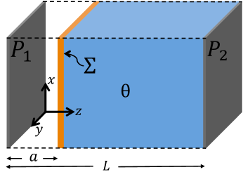
Figure 1: Schematic of the Casimir effect in $\theta$-ED.

To obtain the general solution of Eq. (4) for arbitrary external sources, we introduce the GF matrix $G^{\nu}_{\phantom{\nu}\sigma}\left(x,x^{\prime}\right)$ satisfying

$$\left[\eta^{\mu}_{\phantom{\mu}\nu}\partial^{2}-\tilde{\theta}\delta\left(\Sigma\right)\epsilon^{3\mu\alpha}_{\phantom{3\mu\alpha}\nu}\partial_{\alpha}\right]G^{\nu}_{\phantom{\nu}\sigma}\left(x,x^{\prime}\right)=4\pi\eta^{\mu}_{\phantom{\mu}\sigma}\delta\left(x-x^{\prime}\right),$$ (6)

together with the BCs in Eq. (5). Next we solve Eq. (6) along the same lines introduced in Ref. [15] for the static case. A similar technique has been used in Refs. [16, 17] to study two parallel planes represented by two $\delta$-functions. The GF we consider has translational invariance in the directions parallel to $\Sigma$, that is in the transverse $x$ and $y$ directions, while this invariance is broken in the $z$ direction. Exploiting this symmetry we can write

$$G_{\phantom{\mu}\nu}^{\mu}\left(x,x^{\prime}\right)=4\pi\int\frac{d^{2}\mathbf{p}}{\left(2\pi\right)^{2}}e^{i\mathbf{p}\cdot\textbf{R}}\int\frac{d\omega}{2\pi}e^{-i\omega(t-t^{\prime})}g_{\phantom{\mu}\nu}^{\mu}\left(z,z^{\prime}\right),$$ (7)

where $\textbf{R}=(x-x^{\prime},\;y-y^{\prime})$ and $\mathbf{p}=(p_{x},p_{y})$ is the momentum parallel to $\Sigma$ [18]. In Eq. (7) we have omitted the dependence of the reduced GF $g_{\phantom{\mu}\nu}^{\mu}$ on $\omega$ and $\mathbf{p}$. Due to the antisymmetry of the Levi-Cività symbol, the partial derivative appearing in the second term of Eq. (6) does not introduce derivatives with respect to $z$. This allows us to write the equation for the reduced GF $g_{\phantom{\nu}\sigma}^{\nu}(z,z^{\prime})$ as

$$\left[\eta_{\phantom{\mu}\nu}^{\mu}\partial^{2}+i\tilde{\theta}\delta\left(\Sigma\right)\epsilon_{\phantom{3\mu\alpha}\nu}^{3\mu\alpha}p_{\alpha}\right]g_{\phantom{\nu}\sigma}^{\nu}\left(z,z^{\prime}\right)=\eta_{\phantom{\mu}\sigma}^{\mu}\delta\left(z-z^{\prime}\right),$$ (8)

where now $\partial^{2}=\mathbf{p}^{2}-\omega^{2}-\partial_{z}^{2}$ and $p^{\alpha}=\left(\omega,\mathbf{p},0\right)$. In solving Eq. (8) we employ a method similar to that used for obtaining the GF for the one-dimensional $\delta$-function potential in quantum mechanics, where the free GF is used for integrating the GF equation with $\delta$-interaction. Here the free GF we use is the reduced GF for two parallel conducting surfaces placed at $z=0$ and $z=L$, which is the solution of $\partial^{2}\mathfrak{g}\left(z,z^{\prime}\right)=\delta\left(z-z^{\prime}\right)$ satisfying the BC $\mathfrak{g}\left(0,z^{\prime}\right)=\mathfrak{g}\left(L,z^{\prime}\right)=0$, namely:

$$\mathfrak{g}\left(z,z^{\prime}\right)=\frac{\sin\left[pz_{<}\right]\sin\left[p\left(L-z_{>}\right)\right]}{p\sin\left[pL\right]},$$ (9)

where $z_{>}$ ($z_{<}$) is the greater (lesser) of $z$ and $z^{\prime}$, and $p=\sqrt{\omega^{2}-\textbf{p}^{2}}$. Now, Eq. (8) can be directly integrated using the free GF (9) together with the properties of the $\delta$-function, reducing the problem to a set of coupled algebraic equations,

$$g^{\mu}_{\phantom{\mu}\sigma}\left(z,z^{\prime}\right)=\eta^{\mu}_{\phantom{\mu}\sigma}\mathfrak{g}\left(z,z^{\prime}\right)-i\tilde{\theta}\epsilon^{3\mu\alpha}_{\phantom{3\mu\alpha}\nu}p_{\alpha}\mathfrak{g}\left(z,a\right)g^{\nu}_{\phantom{\nu}\sigma}\left(a,z^{\prime}\right).$$ (10)

Note that the continuity of $\mathfrak{g}$ at $z=z^{\prime}$ implies the continuity of $g^{\mu}_{\phantom{\mu}\sigma}$ there, and the discontinuity of $\partial_{z}\mathfrak{g}$ at the same point yields the corresponding discontinuity of $\partial_{z}g^{\mu}_{\phantom{\mu}\sigma}$, in accordance with the BC (5). We write the general solution to Eq. (10) as the sum of two terms, $g^{\mu}_{\phantom{\mu}\nu}\left(z,z^{\prime}\right)=\eta^{\mu}_{\phantom{\mu}\nu}\mathfrak{g}\left(z,z^{\prime}\right)+g^{\mu}_{\theta\nu}\left(z,z^{\prime}\right)$. The first term provides the propagation in the absence of the TI. The second, to be called the reduced $\theta$-GF, which can be shown to be

$$g^{\mu}_{\theta\nu}\left(z,z^{\prime}\right)=\tilde{\theta}\mathfrak{g}\left(a,a\right)\left[p^{\mu}p_{\nu}-\left(\eta^{\mu}_{\phantom{\mu}\nu}+n^{\mu}n_{\nu}\right)p^{2}\right]P\left(z,z^{\prime}\right)$$

$$+\,i\,\epsilon^{\mu\phantom{\nu}\alpha 3}_{\phantom{\mu}\nu}p_{\alpha}P\left(z,z^{\prime}\right),$$ (11)

encodes the TME due to the topological $\theta$-term. Here

$$P\left(z,z^{\prime}\right)=-\tilde{\theta}\frac{\mathfrak{g}\left(z,a\right)\mathfrak{g}\left(a,z^{\prime}\right)}{1-p^{2}\tilde{\theta}^{2}\mathfrak{g}^{2}\left(a,a\right)}.$$ (12)

In the static limit ($\omega=0$), our result (11) reduces to the one reported in Ref. [15]. Clearly, the full GF matrix $G^{\mu}_{\phantom{\mu}\nu}\left(x,x^{\prime}\right)$ can also be written as the sum of two terms, $G^{\mu}_{\phantom{\mu}\nu}\left(x,x^{\prime}\right)=\eta^{\mu}_{\phantom{\mu}\nu}\mathcal{G}\left(x,x^{\prime}\right)+G^{\mu}_{\theta\nu}\left(x,x^{\prime}\right)$. We remark in passing that the reciprocity relation for the GF, $G_{\mu\nu}(x,x^{\prime})=G_{\nu\mu}(x^{\prime},x)$, is a direct consequence of the property $g_{\mu\nu}\left(z,z^{\prime},p^{\alpha}\right)=g_{\nu\mu}\left(z^{\prime},z,-p^{\alpha}\right)$.

3 III. The vacuum stress-energy tensor

In the previous section we showed that the $\theta$-term modifies the behaviour of the fields at the surface $\Sigma$ only. This suggests that, for the bulk regions, the stress-energy tensor (SET) for $\theta$-ED has the same form as that in standard electrodynamics. In fact, in Ref. [15] we explicitly computed the SET and verified the latter. As it turns out the SET can be cast in the from:

$$T^{\mu\nu}=\frac{1}{4\pi}\left(-F^{\mu\lambda}F^{\nu}_{\phantom{\nu}\lambda}+\frac{1}{4}\eta^{\mu\nu}F_{\alpha\beta}F^{\alpha\beta}\right).$$ (13)

Clearly this tensor is traceless, i.e., $T^{\mu}_{\phantom{\mu}\mu}=0$ and its divergence is

$$\partial_{\mu}T^{\mu\nu}=-F^{\nu}_{\phantom{\nu}\lambda}j^{\lambda}-(\tilde{\theta}/4\pi)\delta\left(\Sigma\right)n_{\mu}F^{\nu}_{\phantom{\nu}\lambda}\tilde{F}^{\mu\lambda}.$$ (14)

As expected, the SET it is not conserved at $\Sigma$ because of the TME which induces effective charge and current densities there.

Now we address the vacuum expectation value of the SET, to which we will refer simply as the vacuum stress (VS). The local approach to compute the VS was initiated by Brown and Maclay who calculated the renormalised stress tensor by means of GF techniques [14, 19]. In there, the VS can be obtained from appropriate derivatives of the GF, in virtue of Eq. (2.1E) from Ref. [20],

$$G^{\mu\nu}\left(x,x^{\prime}\right)=-i\left<0\right|\hat{\mathcal{T}}A^{\mu}\left(x\right)A^{\nu}\left(x^{\prime}\right)\left|0\right>.$$ (15)

Using the standard point splitting technique and taking the vacuum expectation value of the SET (13) we find

$$\left<T^{\mu\nu}\right>=\frac{i}{4\pi}\lim_{x\rightarrow x^{\prime}}\Big{[}-\partial^{\mu}\partial^{\prime\nu}G^{\lambda}_{\phantom{\lambda}\lambda}+\partial^{\mu}\partial_{\lambda}^{\prime}G^{\lambda\nu}+\partial^{\lambda}\partial^{\prime\nu}G^{\mu}_{\phantom{\mu}\lambda}$$

$$-\,\partial^{\prime\lambda}\partial_{\lambda}G^{\mu\nu}+\frac{1}{2}\eta^{\mu\nu}\left(\partial^{\alpha}\partial_{\alpha}^{\prime}G^{\lambda}_{\phantom{\lambda}\lambda}-\partial^{\alpha}\partial_{\beta}^{\prime}G^{\beta}_{\phantom{\beta}\alpha}\right)\Big{]},$$ (16)

where we have omitted the dependence of $G^{\mu\nu}$ on $x$ and $x^{\prime}$. This result can be further simplified as follows. Since the GF is written as the sum of two terms, then the VS can also be written in the same way, i.e.,

$$\left<T^{\mu\nu}\right>=\left<t^{\mu\nu}\right>+\left<T^{\mu\nu}_{\theta}\right>.$$ (17)

The first term,

$$\left<t^{\mu\nu}\right>=\frac{1}{4\pi i}\lim_{x\rightarrow x^{\prime}}\left(2\partial^{\mu}\partial^{\prime\nu}-\frac{1}{2}\eta^{\mu\nu}\partial^{\lambda}\partial_{\lambda}^{\prime}\right)\mathcal{G}\left(x,x^{\prime}\right),$$ (18)

is the VS in the absence of the TI. In obtaining Eq. (18) we use that the GF is diagonal when the TI is absent, i.e. it is equal to $\eta^{\mu}_{\phantom{\mu}\nu}\mathcal{G}\left(x,x^{\prime}\right)$. The second term, to which we will refer as the $\theta$ vacuum stress ($\theta$-VS), can be simplified since the $\theta$-GF satisfies the Lorentz gauge condition $\partial_{\mu}G^{\mu\nu}_{\theta}=0$. The proof follows from the reduced GF of Eq. (11):

$$\partial_{\mu}G^{\mu}_{\theta\nu}\left(x,x^{\prime}\right)\propto\int\int p_{\mu}g_{\theta\nu}^{\mu}\left(z,z^{\prime}\right),$$ (19)

which vanishes given that $\epsilon_{\phantom{\mu}\nu}^{\mu\phantom{\nu}\alpha 3}p_{\mu}p_{\alpha}=0$ and $p_{\mu}n^{\mu}=0$. With the previous result the $\theta$-VS can be written as

$$\left<T^{\mu\nu}_{\theta}\right>=\frac{1}{4\pi i}\lim_{x\rightarrow x^{\prime}}\left[\partial^{\mu}\partial^{\prime\nu}G_{\theta}+\partial^{\prime\lambda}\partial_{\lambda}\left(G^{\mu\nu}_{\theta}-\frac{1}{2}\eta^{\mu\nu}G_{\theta}\right)\right],$$ (20)

where $G_{\theta}=G^{\mu}_{\theta\mu}$ is the trace of the $\theta$-GF. This result exhibits the vanishing of the trace at quantum level, i.e., $\eta_{\mu\nu}\left<T^{\mu\nu}_{\theta}\right>=0$. For the simplest situation in which the SET is conserved, one can verify that $\partial_{\nu}\left<T^{\mu\nu}\right>=\left<\partial_{\nu}T^{\mu\nu}\right>=0$. However, as pointed out by Deutsch and Candelas [20], this identity need not be a rule. The problem at hand is an example of this, since $\left<\partial_{\nu}T^{\mu\nu}_{\theta}\right>=(\tilde{\theta}/8\pi i)\delta(\Sigma)\eta^{\mu 3}\epsilon^{\sigma\nu\alpha\beta}\lim_{x\rightarrow x^{\prime}}\partial_{\sigma}\partial^{\prime}_{\alpha}G_{\theta\nu\beta}$, which can be shown to be different from $\partial_{\nu}\left<T_{\theta}^{\mu\nu}\right>$.

4 IV. The Casimir Effect

Now we consider the problem of calculating the renormalised VS $\left<T^{\mu\nu}\right>_{\mathrm{ren}}$, which is obtained as the difference between the VS in the presence of boundaries and that of the free vacuum. In the standard case ($\theta=0$), Brown and Maclay [14] obtained that it is uniform between the plates,

$$\left<t^{\mu\nu}\right>_{\mathrm{ren}}=-\frac{\pi^{2}}{720L^{4}}\left(\eta^{\mu\nu}+4n^{\mu}n^{\nu}\right),$$ (21)

with $L$ the distance between the plates. The Casimir stress on the plates was obtained by differentiating the Casimir energy ${\mathcal{E}}_{L}=L\left<t^{00}\right>_{\mathrm{ren}}=-\pi^{2}/720L^{3}$ with respect to $L$, i.e., $F_{L}=-d{\mathcal{E}}_{L}/dL=-\pi^{2}/240L^{4}$.

Now our concern is to calculate the renormalised $\theta$-VS (20) for our Casimir system. We proceed along the lines of Refs. [14, 20]. From Eq. (20), together with the symmetry of the problem we find that the $\theta$-VS can be written as

$$\left<T^{\mu\nu}_{\theta}\right>=i\tilde{\theta}\int\frac{d^{2}\textbf{p}}{(2\pi)^{2}}\int\frac{d\omega}{2\pi}\left(p^{\mu}p^{\nu}+n^{\mu}n^{\nu}p^{2}\right)\times$$

$$\mathfrak{g}\left(a,a\right)\lim_{z\rightarrow z^{\prime}}\left(p^{2}+\partial^{\prime}_{z}\partial_{z}\right)P\left(z,z^{\prime}\right),$$ (22)

where we have used $\partial^{\mu}=(-i\omega,i\textbf{p},\partial_{z})$. In deriving this result we used the Fourier representation of the GF in Eq. (7) together with the solution for the reduced $\theta$-GF given by Eq. (11). From the result (22) we calculate the renormalised $\theta$-VS, which is given by $\left<T^{\mu\nu}_{\theta}\right>_{\mathrm{ren}}=\left<T^{\mu\nu}_{\theta}\right>-\left<T^{\mu\nu}_{\theta}\right>_{\mathrm{vac}}$, where the first (second) term is the $\theta$-VS in the presence (absence) of the plates [20]. When the plates are absent, the reduced GF we have to use to compute the $\theta$-VS in the region $[0,L]$ is that of the free-vacuum, $\mathfrak{g}_{0}\left(z,z^{\prime}\right)=(i/2p)\exp(ip|z-z^{\prime}|)$ [18], from which we find that $\lim_{z\rightarrow z^{\prime}}\partial_{z}\partial_{z}^{\prime}P_{0}\left(z,z^{\prime}\right)=-p^{2}\lim_{z\rightarrow z^{\prime}}P_{0}\left(z,z^{\prime}\right)$, thus implying that the integrand in Eq. (22) vanishes. The function $P_{0}$ is given by Eq. (12) when the free-vacuum reduced GF $\mathfrak{g}(z,z^{\prime})$ is replaced by $\mathfrak{g}_{0}(z,z^{\prime})$. Therefore we conclude that $\left<T^{\mu\nu}_{\theta}\right>_{vac}=0$.

Next we compute $\left<T^{\mu\nu}_{\theta}\right>_{\mathrm{ren}}=\left<T^{\mu\nu}_{\theta}\right>$ starting from Eq. (22). From the symmetry of the problem, the components of the stress along the plates, $\left<T^{11}_{\theta}\right>$ and $\left<T^{22}_{\theta}\right>$, are equal. In addition, from the mathematical structure of Eq. (22) we find the relation $\left<T^{00}_{\theta}\right>=-\left<T^{11}_{\theta}\right>$. These results, together with the traceless nature of the SET, allow us to write the renormalised $\theta$-VS in the form

$$\left<T^{\mu\nu}_{\theta}\right>_{\mathrm{ren}}=\left(\eta^{\mu\nu}+4n^{\mu}n^{\nu}\right)\tau(\theta,z)\;,$$ (23)

where

$$\tau(\theta,z) = i\tilde{\theta}\int\frac{d^{2}\textbf{p}}{(2\pi)^{2}}\int\frac{d\omega}{2\pi}\omega^{2}\mathfrak{g}\left(a,a\right)\times$$ (24)

$$\lim_{z\rightarrow z^{\prime}}\left(p^{2}+\partial^{\prime}_{z}\partial_{z}\right)P\left(z,z^{\prime}\right).$$

Note that our $\theta$-VS exhibits the same tensor structure as the result obtained by Brown and Maclay (21), but we obtain a $z$-dependent VS since the SET is not conserved at $\Sigma$. To understand better $\tau(\theta,z)$, we compute the limit of the integrand in Eq. (24). Using Eq. (9) we obtain

$$\lim_{z\rightarrow z^{\prime}}\left(p^{2}+\partial_{z}\partial_{z}^{\prime}\right)P\left(z,z^{\prime}\right)=-\frac{\tilde{\theta}}{1-\tilde{\theta}^{2}p^{2}\mathfrak{g}^{2}\left(a,a\right)}\times$$

$$\left\{\frac{\sin^{2}\left[p\left(L-a\right)\right]}{\sin^{2}\left[pL\right]}H\left(a-z\right)+\frac{\sin^{2}\left[pa\right]}{\sin^{2}\left[pL\right]}H\left(z-a\right)\right\}.$$ (25)

To evaluate the integral in Eq. (24) we first write the momentum element as $d^{2}\textbf{p}=|\textbf{p}|d|\textbf{p}|d\vartheta$ and integrate $\vartheta$. Next, we perform a Wick rotation such that $\omega\rightarrow i\zeta$, then replace $\zeta$ and $|\textbf{p}|$ by plane polar coordinates $\zeta=\xi\cos\varphi$, $|\textbf{p}|=\xi\sin\varphi$ and finally integrate $\varphi$. The renormalised $\theta$-VS in Eq. (23) then becomes

$$\left<T^{\mu\nu}_{\theta}\right>_{\mathrm{ren}}=-\frac{\pi^{2}}{720L^{4}}\left(\eta^{\mu\nu}+4n^{\mu}n^{\nu}\right)\times$$

$$\left[u(\theta,\chi)H\left(a-z\right)+u(\theta,1-\chi)H\left(z-a\right)\right],$$ (26)

where

$$u(\theta,\chi)=\frac{120}{\pi^{4}}\int_{0}^{\infty}\frac{\tilde{\theta}^{2}\xi^{3}\mbox{\small sh}\left[\xi\chi\right]\mbox{\small sh}^{3}\left[\xi\left(1-\chi\right)\right]\mbox{\small sh}^{-3}\left[\xi\right]}{1+\tilde{\theta}^{2}\mbox{\small sh}^{2}\left[\xi\chi\right]\mbox{\small sh}^{2}\left[\xi\left(1-\chi\right)\right]\mbox{\small sh}^{-2}\left[\xi\right]}d\xi,$$ (27)

with $\mbox{\small sh}(x)=\sinh(x)$ and $\chi=a/L$ with $0<\chi<1$. Physically, we interpret the function $u(\theta,\chi)$ as the ratio between the renormalised $\theta$-energy density in the vacuum region $[0,a)$ and that of the renormalised energy density in the absence of the TI, $\left<t^{00}\right>_{\mathrm{ren}}$. The function $u(\theta,1-\chi)$ has an analogous interpretation for the bulk region of the TI $(a,L]$. This shows that the energy density is constant in the bulk regions, however a simple discontinuity arises at $\Sigma$, i.e., $\partial_{z}\left<T^{00}_{\theta}\right>_{\mathrm{ren}}\propto\delta(\Sigma)$. The Casimir energy ${\cal E}={\cal E}_{L}+{\cal E}_{\theta}$ is defined as the energy per unit of area stored in the electromagnetic field between the plates. To obtain it we must integrate the contribution from the $\theta$-energy density.

$$\mathcal{E}_{\theta}=\int_{0}^{L}dz\left<T^{00}_{\theta}\right>_{\mathrm{ren}}={\mathcal{E}}_{L}\left[\chi u(\theta,\chi)+(1-\chi)u(\theta,1-\chi)\right],$$ (28)

recalling that $\mathcal{E}_{L}$ is the Casimir energy in the absence of the TI. The first term corresponds to the energy stored in the electromagnetic field between $P_{1}$ and $\Sigma$, while the second term is the energy stored in the bulk of the TI. The ratio $\mathcal{E}_{\theta}/{\mathcal{E}}_{L}$ as a function of $\chi$ for different values of $\theta$ (appropriate for TIs [11]) is plotted in Fig. 2.

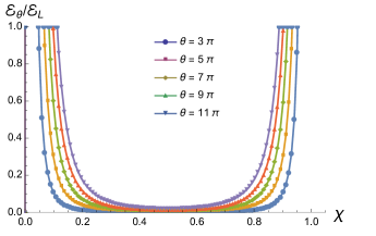
Figure 2: The ratio $\mathcal{E}_{\theta}/\mathcal{E}_{L}$ as a function of the dimensionless distance $\chi=a/L$, for different values of $\theta$.

4.1 IV-a The Casimir stress on the $\theta$-piston

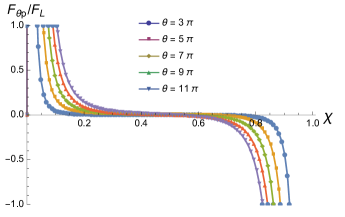
Figure 3: The Casimir stress on the $\theta$-piston in units of $F_{L}$ as a function of $\chi$, for different values of $\theta$.

The setup known in the literature as the Casimir piston consists of a rectangular box of length $L$ divided by a movable mirror (piston) at a distance $a$ from one of the plates [21]. The net result is that the Casimir energy in each region generates a force on the piston pulling it towards the nearest end of the box. Here we consider a similar setup, which we have called the $\theta$-piston, in which the piston is the TI. Since the surface $\Sigma$ changes the energy density of the electromagnetic field in the bulk regions, an effective Casimir stress acts upon $\Sigma$. This can be obtained as $F_{\theta p}=-d\mathcal{E}_{\theta}/da$. The result is

$$\frac{F_{\theta p}}{F_{L}}=-\frac{1}{3}\frac{d}{d\chi}\left[\chi u(\theta,\chi)+(1-\chi)u(\theta,1-\chi)\right],$$ (29)

where $F_{L}$ is the Casimir stress between the two perfectly reflecting plates in the absence of the TI. Figure 3 shows the Casimir stress on $\Sigma$ in units of $F_{L}$ as a function of $\chi$ for different values of $\theta$. We observe that this force pulls the boundary $\Sigma$ towards the closer of the two fixed walls $P_{1}$ or $P_{2}$, similarly to the conclusion in Ref.[21].

4.2 IV-b Casimir stress between $P_{1}$ and $\Sigma$, when $L\rightarrow\infty$

Now let us consider the limit where the plate $P_{2}$ is sent to infinity, i.e., $L\rightarrow\infty$. This configuration corresponds to a perfectly conducting plate $P_{1}$ in vacuum, and a semi-infinite TI located at a distance $a$. Here the plate and the TI exert a force upon each other. The Casimir energy (28) in the limit $L\rightarrow\infty$ takes the form $\mathcal{E}_{\theta}^{L\rightarrow\infty}={\mathcal{E}}_{a}R(\theta)$, with ${\mathcal{E}}_{a}=-\pi^{2}/720a^{3}$, and the function

$$R(\theta)=\frac{120}{\pi^{4}}\int_{0}^{\infty}\xi^{3}\frac{\tilde{\theta}^{2}}{1+\tilde{\theta}^{2}e^{-2\xi}\sinh^{2}\xi}e^{-3\xi}\sinh\xi d\xi,$$ (30)

is $a$-independent and bounded by its $\theta\rightarrow\pm\infty$ limit, i.e.,

$$R(\theta)\leq\frac{120}{\pi^{4}}\int_{0}^{\infty}\xi^{3}\frac{e^{-\xi}}{\sinh\xi}d\xi=1.$$ (31)

Thus, for this case, the energy stored in the electromagnetic field is bounded by the Casimir energy between two parallel conducting plates at a distance $a$, i.e., $\mathcal{E}_{\theta}^{L\rightarrow\infty}\leq{\mathcal{E}}_{a}$. Physically this implies that in the $\theta\rightarrow\infty$ limit the surface of the TI mimics a conducting plate, which is analogous to Schwinger’s prescription for describing a conducting plate as the $\varepsilon\rightarrow\infty$ limit of material media [18]. These results, which stem from our Eqs. (11) and (12), agree with those obtained in the global energy approach which uses the reflection matrices containing the Fresnel coefficients as in Ref. [11], when the appropriate limits to describe an ideal conductor at $P_{1}$ and a purely topological surface at $\Sigma$ are taken into account. The calculation, however, is too long to be shown here. Taking the derivative with respect to $a$ we find that the plate and the TI exert a force (in units of $F_{a}=-\pi^{2}/240a^{4}$) of attraction upon each other given by $f_{\theta}=F^{L\rightarrow\infty}_{\theta}/F_{a}=R(\theta)$. Numerical results for $f_{\theta}$ for different values of $\theta$ are presented in Table 1.

$\theta$	$\pm 7\pi$	$\pm 15\pi$	$\pm 23\pi$	$\pm 31\pi$	$\pm 39\pi$
$f_{\theta}$	0.0005	0.0025	0.0060	0.0109	0.0172

.

Table 1: Normalized force $f_{\theta}=F^{L\rightarrow\infty}_{\theta}/F_{a}=R(\theta)$ for different values of $\theta$.

5 V. Conclusions and Outlook

In this letter we have used the stress-energy tensor to compute the Casimir energy and stress for the system shown in Fig. 1. The setup consists of a slab of a coated topological insulator (TI) of constant topological magnetoelectric polarisability $\theta$ in the region $a<z<L$, which partially fills the space between two perfectly reflecting parallel plates. In a first approach, we ignore features that are relevant in experimental situations, such as the optical properties of TIs and temperature effects, which can be taken into account including these parameters in the Green’s function according to standard methods Refs. [3, 4, 18]. The system is well described by the action of $\theta$ electrodynamics given in Eq. (1). In this work, we obtained the renormalised vacuum stress from (derivatives of) the corresponding Green’s function (GF) of the problem. To this end we require the time dependent GF, for which we extended our results of Ref. [15], which dealt with the static case. This GF can be exactly calculated because the TI introduces a localised discontinuity in the equations of motion along the $z$ direction, while the dependence in time and in the remaining coordinates is invariant under the respective translations. We considered two cases: (1) the $\theta$-piston, defined in the interval $0<z<L$. The contribution to the Casimir energy ${\mathcal{E}}={\mathcal{E}}_{L}+{\mathcal{E}}_{\theta}$, that arises from the TI, ${\mathcal{E}}_{\theta}$, is plotted in Fig. 2, in units of ${\mathcal{E}}_{L}$, as a function of the reduced length $\chi$ and for various values of $\theta$. The Casimir stress on the boundary $\Sigma$, $F_{\theta p}=-d\mathcal{E}/da$, is plotted in Fig. 3, in units of $F_{L}$. We observe that this force pulls $\Sigma$ towards the closer of the two fixed walls $P_{1}$ or $P_{2}$, similarly to the conclusion in Ref.[21]. (2) The second case we have considered is the $L\rightarrow\infty$ limit of the $\theta$-piston, which describes the interaction, via the interface $\Sigma$, between the conducting plate $P_{1}$ in vacuum and a semi-infinite TI located at a distance $a$. The corresponding Casimir stress, in units of $F_{a}$, is shown in Table 1, for different values of $\theta$. These results, which rely on the due evaluation of GFs and the renormalised stress-energy tensor, are in perfect agreement with those obtained following the global energy approach of Ref. [11]. We also remark that the discontinuity of the vacuum expectation value of the energy density obtained in Eq. (26) is finite, similar to that in Ref. [17]. Although, in our case, a physical interpretation of such discontinuity is not immediate, it is somehow expected due to the non-conservation of the stress-energy tensor at the $\Sigma$ boundary owing to the self-induced charge and current densities there [15].

A general feature of our analysis is that the TI induces a $\theta$-dependence on the Casimir stress, which could be used to measure $\theta$. Since the Casimir stress has been measured for separation distances in the $0.5-3.0\,\mu$m range [2], these measurements require TIs of width lesser than $0.5\mu$m and an increase of the experimental precision of two to three orders of magnitude. In practice the measurability of $f_{\theta}$ depends on the value of the TMEP, which is quantised as $\theta=(2n+1)\pi,\,n\in\mathbb{Z}$. The particular values $\theta=\pm 7\pi,\pm 15\pi$ are appropriate for the TIs such as Bi_1-xSe_x [22], where we have $f_{\pm 7\pi}\approx 0.0005$ and $f_{\pm 15\pi}\approx 0.0025$, which are not yet feasible with the present experimental precision. This effect could also be explored in TIs described by a higher coupling $\theta$, such as Cr₂O₃. However, this material induces more general magnetoelectric couplings not considered in our model [11].

Although the reported $\theta$-effects of our Casimir systems cannot be observed in the laboratory yet, we have aimed to establish the Green’s function method as an alternative theoretical framework for dealing with the topological magnetoelectric effect of TIs and also as yet another application of the GF method we developed in Ref. [15].

Though not frequently used in the corresponding TIs literature, this method plays an important role in the calculations of the standard Casimir effect, besides its usefulness in many other topics in $\theta$ electrodynamics.

- [1] H. B. G. Casimir, Proc. K. Ned. Akad. Wet. 51, 793 (1948).
- [2] G. Bressi et al, Phys. Rev. Lett. 88, 041804 (2002).
- [3] K. A. Milton, The Casimir effect: Physical Manifestation of Zero-Point Energy (World Scientific, Singapore, 2001).
- [4] M. Bordag, G. L. Klimchitskaya, U. Mohideen and V. M. Mostepanenko, Advances in Casimir effect (Oxford University Press, Great Britain, 2009).
- [5] M. Frank and I. Turan, Phys. Rev. D 74, 033016 (2006); K. A. Milton and Y. J. Ng, Phys. Rev. D 42, 2875 (1990).
- [6] J. Q. Quach, Phys. Rev. Lett. 114, 081104 (2015).
- [7] L. Fu, C. L. Kane, and E. J. Mele, Phys. Rev. Lett. 98, 106803 (2007); Hsieh, D., D. Qian, L. Wray, Y. Xia, Y. S. Hor, R. J. Cava and M. Z. Hasan, Nature 452, 970 (2008).
- [8] X. L. Qi, R. Li, J. Zang and S. C. Zhang, Science 323, 1184 (2009).
- [9] G. Rosenberg and M. Franz, Phys. Rev. B 82, 035105 (2010).
- [10] J. Maciejko, X. L. Qi, H. D. Drew and S. C. Zhang, Phys. Rev. Lett. 105, 166803 (2010).
- [11] A. G. Grushin and A. Cortijo, Phys. Rev. Lett. 106, 020403 (2011); A. G. Grushin, P. Rodriguez-Lopez and A. Cortijo, Phys. Rev. B 84, 045119 (2011).
- [12] Y. N. Obukhov and F. W. Hehl, Phys. Lett. A 341, 357 (2005); L. Huerta and J. Zanelli, Phys. Rev. D 85, 085024 (2012); L. Huerta, Phys. Rev. D 90, 105026 (2014).
- [13] X. L. Qi and S. C. Zhang Rev. Mod. Phys. 83, 1057 (2011).
- [14] L. S. Brown and G. J. Maclay, Phys. Rev. 184, 1272 (1969).
- [15] A. Martín-Ruiz, M. Cambiaso and L. F. Urrutia, Phys. Rev. D 92, 125015 (2015); Phys. Rev. D 93, 045022 (2016).
- [16] M. Bordag, D. Hennig and D. Robaschik, J. Phys. A 25, 4483 (1992).
- [17] K. A. Milton, J. Phys. A 37, 6391 (2004).
- [18] J. Schwinger, L. DeRaad, K. Milton and W. Tsai, “Classical Electrodynamics”, Advanced Book Program, (Perseus Books 1998).
- [19] J. Schwinger, L. DeRaad and K. Milton, Ann. Phys. (N.Y.) 115, 1 (1978).
- [20] D. Deutsch and P. Candelas, Phys. Rev. D 20, 3063 (1979).
- [21] R. M. Cavalcanti, Phys. Rev. D 69, 065015 (2004).
- [22] X. Zhou, et al, Phys. Rev. A 88, 053840 (2013).