Interband heating processes in a periodically driven optical lattice

Abstract

We investigate multi-“photon” interband excitation processes in an optical lattice that is driven periodically in time by a modulation of the lattice depth. Assuming the system to be prepared in the lowest band, we compute the excitation spectrum numerically. Moreover, we estimate the effective coupling parameters for resonant interband excitation processes analytically, employing degenerate perturbation theory in Floquet space. We find that below a threshold driving strength, interband excitations are suppressed exponentially with respect to the inverse driving frequency. For sufficiently low frequencies, this leads to a rather sudden onset of interband heating, once the driving strength reaches the threshold. We argue that this behavior is rather generic and should also be found in lattice systems that are driven by other forms of periodic forcing. Our results are relevant for Floquet engineering, where a lattice system is driven periodically in time in order to endow it with novel properties like the emergence of a strong artificial magnetic field or a topological band structure. In this context, interband excitation processes correspond to detrimental heating.

I Introduction

Floquet engineering is a form of quantum engineering, where a system is periodically driven in time, such that it behaves as if it was governed by an effective time-independent Hamiltonian with desired properties. This concept has recently been demonstrated successfully in a series of experiments with ultracold atomic quantum gases in driven optical lattices Eckardt (2016). This includes the dynamic localization of a Bose-Einstein condensate in a shaken optical lattice Lignier et al. (2007); Eckardt et al. (2009), “photon”-assisted tunneling against a potential gradient Sias et al. (2008); Ivanov et al. (2008); Alberti et al. (2009); Haller et al. (2010); Ma et al. (2011) and the dynamic control of the bosonic Mott transition in a strongly interacting system Zenesini et al. (2009). The concept of Floquet engineering becomes particularly relevant, when the driven system acquires properties that are qualitatively different from those of the undriven system. A prime example is the realization of artificial magnetic fields, where driven charge-neutral atoms behave as if they had a charge coupling to an effective magnetic field Struck et al. (2011); Aidelsburger et al. (2011); Struck et al. (2012, 2013); Aidelsburger et al. (2013); Miyake et al. (2013); Atala et al. (2014); Jotzu et al. (2014); Kennedy et al. (2015); Aidelsburger et al. (2015).

The idea of Floquet engineering is based on the fact that the time evolution of a quantum system with time-periodic Hamiltonian $\hat{H}(t)=\hat{H}(t+T)$ can be expressed in terms of an effective time-independent Hamiltonian Shirley (1965); Sambe (1973). Namely, the unitary time evolution operator over one driving cycle, from time $t_{0}$ to time $t_{0}+T$, can be written like $\exp(-iT\hat{H}^{F}_{t_{0}}/\hbar)$ in terms of a hermitian operator $\hat{H}^{F}_{t_{0}}$ often called Floquet Hamiltonian. However, the very fact that we can formally define an effective time-independent Hamiltonian is not enough to make the concept of Floquet engineering work. We also have to require that the effective Hamiltonian can be computed theoretically and takes a simple form allowing for a clear interpretation. In an extended system of many interacting particles this condition will typically not be fulfilled exactly. Roughly speaking, the fact that the driving resonantly couples (and, thus, hybridizes) energetically distant states makes the effective Hamiltonian an object much more complex than a typical time-independent Hamiltonian. As a consequence of this lack of energy conservation, it is believed that a generic many-body Floquet system approaches an infinite-temperature-like state in the long-time limit Lazarides et al. (2014); D’Alessio and Rigol (2014). Floquet engineering, nevertheless, works in an approximate sense in parameter regimes, where unwanted resonant coupling is weak and can be neglected on the time scale of the experiment.

In the optical lattice experiments mentioned above, this parameter regime is characterized by two conditions Eckardt et al. (2005). The first one is a low-frequency condition: In order to describe the system in terms of a Hubbard-type tight-binding model with a single Wannier-like orbital in each lattice minimum, one requires the driving frequency to be small compared to the energy gap $\Delta$ that separates excited orbital degrees of freedom,

$$\hbar\omega\ll\Delta.$$ (1)

The second requirement is a high-frequency condition: In order to suppress resonant coupling within the subspace of low-energy orbitals described by the tight-binding model, the driving frequency shall be large compared to the matrix element $J$ for tunneling between neighboring lattice minima and the Hubbard parameter $U$ describing on-site interactions,

$$\hbar\omega\gg U,J.$$ (2)

If resonant coupling both to excited orbital states and within the low-energy tight-binding subspace can be neglected, one can compute the approximate effective Hamiltonian relevant for Floquet engineering from the driven tight-binding model using a high-frequency expansion Goldman and Dalibard (2014); Bukov et al. (2015); Eckardt and Anisimovas (2015); Mikami et al. (2015). This is the standard approach of Floquet engineering, on which the above mentioned optical-lattice experiments are based.

However, both conditions (1) and (2) do not completely prevent unwanted resonant excitation processes, which in the context of Floquet engineering must be viewed as heating. It is therefore crucial to identify the most dominant of these heating processes and to estimate their rates. The validity of the high-frequency approximation, neglecting resonant excitations within the low-energy Hubbard description, has been studied for various scenarios in references Eckardt et al. (2005); Eckardt and Holthaus (2007, 2008); Poletti and Kollath (2011); Eckardt and Anisimovas (2015); Genske and Rosch (2015); Bilitewski and Cooper (2015a, b); Bukov et al. (2015); Canovi et al. (2016). For systems with local energy bound, which includes the fermionic Hubbard model, it has been shown that the heating rates decrease exponentially with the driving frequency Kuwahara et al. (2016); Mori et al. (2015); Abanin et al. (2015a, b). In this paper, we will address the validity of the low-frequency approximation, where the resonant coupling to excited orbital states is neglected. Previous work includes theoretical studies of resonant inter-orbital coupling due to both single-particle processes Drese and Holthaus (1997); Lacki and Zakrzewski (2013); Holthaus (2015) and two-particle scattering Sowiński (2012); Choudhury and Mueller (2014, 2015). Recently multi-photon interband excitations have also been observed experimentally and explained theoretically by single-particle processes Weinberg et al. (2015).

In the following we will systematically investigate heating due to single-particle multi-photon interband excitation processes in a one-dimensional optical lattice that is driven by a modulation of the lattice depth like in the experiments described in references Alberti et al. (2009); Ma et al. (2011). For that purpose, we will study interband excitation processes numerically and compare these results to analytical estimates that we obtain using perturbation theory within the Floquet picture. The latter indicate that heating rates are suppressed exponentially for small driving frequencies as long as the driving amplitude remains below a threshold value.

II System

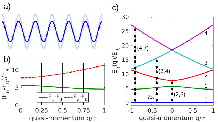
Figure 1: Optical lattice of modulated lattice depth (a). Energy difference between the first/second excited band and the lowest band versus quasimomentum (b) and band structure (c) for a static lattice of depth $V_{0}/E_{R}=10$. The label $(b,n)$ denotes the resonance condition $E_{n}(k)-E_{0}(k)=n\hbar\omega$ for an $n$ “photon” transition from the lowest to the $b$th band.

We consider ultracold atoms in a one-dimensional optical lattice, with the lattice depth modulated sinusoidally in time [Fig. 1(a)]. It is described by the single-particle Hamiltonian

$$\hat{H}(t)=-\frac{\hbar^{2}}{2m}\partial_{x}^{2}+V_{0}[1+\alpha\sin(\omega t)]\sin^{2}(k_{L}x)$$ (3)

where $m$ denotes the particle mass, $V_{0}$ the average lattice depth, $\alpha$ the dimensionless amplitude of the modulation of the lattice depth. The lattice constant $a=\pi/k_{L}$ is determined by the wave number $k_{L}$ of the laser used to create the optical lattice. Using the recoil energy $E_{R}=\frac{\hbar^{2}k_{L}^{2}}{2m}$, corresponding to the kinetic energy needed to localize a particle on the length $a$, as the unit of energy the system is described by three dimensionless parameters, the lattice depth $V_{0}/E_{R}$, the driving amplitude $\alpha$ and the driving frequency $\hbar\omega/E_{R}$. For convenience, we assume periodic boundary conditions, with $M$ denoting the number of lattice sites. Since we are interested in single-particle excitation effects, we do not need to specify the potential along spatial directions other than $x$ by assuming the transverse dynamics separates.

The invariance of the lattice potential with respect to discrete translations $x\to x+a$ implies that quasimomentum $q$, i.e. momentum $p$ modulo the reciprocal lattice constant $2\pi/a$, is conserved. Thus, when describing the system in the basis of momentum eigenstates $|p\rangle$ with wave functions

$$\langle x|p\rangle=\frac{1}{\sqrt{Ma}}e^{ipx},$$ (4)

it is convenient to decompose the momentum wave number like

$$p=q+\beta\frac{2\pi}{a},\quad\text{with}\quad-\frac{\pi}{a}<q\leq\frac{\pi}{a}\quad\text{and}\quad\beta\in\mathbb{Z}.$$ (5)

The wavenumber $q$ can take discrete values that comply with the boundary conditions of the system. With respect to the momentum eigenstates, the Hamiltonian possesses the matrix elements

$$\big{\langle}q^{\prime}+\beta^{\prime}\frac{2\pi}{a}\big{|}\hat{H}^{\prime}(t)\big{|}q+\beta\frac{2\pi}{a}\big{\rangle}=\delta_{q^{\prime},q}\,h_{\beta^{\prime}\beta}(q,t)E_{\text{R}},$$ (6)

that are diagonal with respect to $q$, where

$$h_{\beta^{\prime}\beta}(q,t) = \delta_{\beta^{\prime}\beta}(qa/\pi+2\beta)^{2}$$

$$+\,\frac{1}{4}\frac{V_{0}}{E_{R}}[1+\alpha\sin(\omega t)](\delta_{\beta^{\prime},\beta+1}+\delta_{\beta^{\prime},\beta-1}).$$

The eigenstates

$$|bq\rangle=\sum_{\beta}u_{b\beta}(q)|q+\beta 2\pi/a\rangle$$ (8)

of the undriven Hamiltonian ($\alpha=0$) are labeled by the quasimomentum quantum number $q$ and the band index $b=0,1,2,\ldots$. Their coefficients $u_{b\beta}(q)$ and energies $E_{b}(q)$ are deterimined by the eigenvalue problem

$$\sum_{\beta^{\prime}}E_{R}h_{\beta\beta^{\prime}}(q)u_{b\beta^{\prime}}=E_{b}(q)u_{b\beta}.$$ (9)

Their wave functions are Bloch waves given by $\langle x|bq\rangle=e^{iqx}\sum_{\beta}u_{b\beta}(q)e^{i\beta(2\pi/a)x}\equiv e^{iqx}u_{bq}(x)$, with $u_{bq}(x+a)=u_{bq}(x)$. The band structure $E_{b}(q)$ of the undriven system with $V_{0}/E_{R}=10$ is plotted in Fig. 1(c). Figure 1 (b), moreover, shows the energy differences between the lowest band the first two excited bands.

III Excitation spectrum

We now assume that the system is initially prepared in a Bloch state $|0q\rangle$ of the lowest band and investigate excitations to higher-lying bands when the driving is switched on at $t=0$. For that purpose we integrate the time-dependent Schrödinger equation

$$i\hbar\dot{u}_{\beta}(t)=E_{R}\sum_{\beta^{\prime}}h_{\beta^{\prime}\beta}(q,t)u_{\beta^{\prime}}(t)$$ (10)

over a time span of $\Delta t$, starting from the initial state $u_{\beta}(t=0)=u_{0\beta}(q)$. During the time evolution the state of the system is given by

$$|\psi(t)\rangle=\sum_{\beta}u_{\beta}(t)\big{|}q+\beta\frac{2\pi}{a}\big{\rangle}.$$ (11)

Assuming the recoil energy of $E_{R}=3.33\cdot 2\pi\hbar$ kHz, which is a typical value for experiments with Rubidium 87 atoms, we choose a time span $\Delta t=20$ ms.

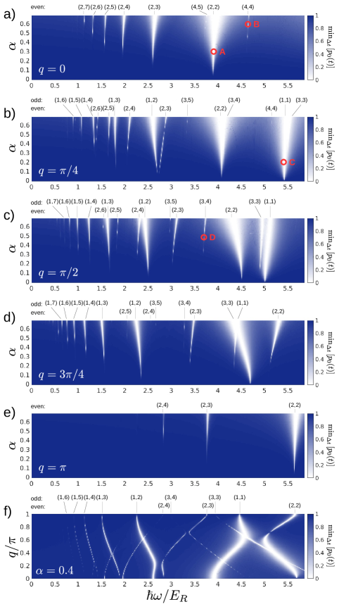
Figure 2: Excitation spectrum: Minimum probability $\min_{\Delta t}[p_{0}(t)]$ to occupy the initial state $|0q\rangle$ during a time span of $\Delta t=20$ ms, plotted versus driving frequency $\hbar\omega/E_{R}$ and either driving amplitude $\alpha$ (a-e) or quasimomentum $q$ (f). The parameters are $V_{0}/E_{R}=10$, $E_{R}=3.33\cdot 2\pi\hbar$ kHz, and $q$ or $\alpha$ as indicated in each panel. Resonances corresponding to an $n$-“photon” transition from band 0 to $b$ are visible as white stripes and labeled by $(b,n)$. For the points marked by $A$, $B$, $C$, $D$, the evolution of the probabilities $p_{b}(t)$ is depicted in panels (a), (b), (c), (d) of Fig. 3, respectively.

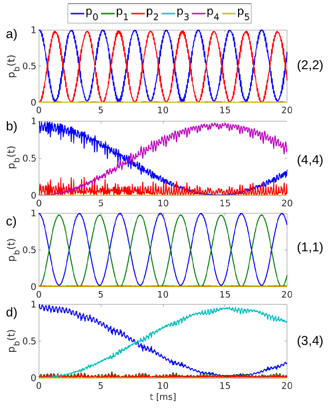
Figure 3: Time evolution of the populations $p_{b}(t)$ of the six lowest bands. From top to bottom the four subplots correspond to the parameters marked by A, B, C, and D marked in Fig. 2, respectively.

The probability to find the system in band $b$ is given by the squared overlap

$$p_{b}(t)=|\langle\psi(t)|bq\rangle|^{2}=\Big{|}\sum_{\beta}u^{*}_{\beta}(t)u_{b\beta}(q)\Big{|}^{2}.$$ (12)

In Fig. 2 we plot the minimal overlap $\min_{\Delta t}[p_{0}(t)]$ with lowest band recorded during the time span $\Delta t$ versus the driving frequency $\hbar\omega/E_{R}$ and either the driving amplitude $\alpha$ or the quasimomentum $q$ for $V_{0}/E_{R}=10$. We can clearly observe resonances, where a light color indicates a significant transfer out of the lowest band. We have labeled $n$-“photon” resonances to band $b$ by $(b,n)$. Such a resonance is expected to occur, roughly, when

$$n\hbar\omega\approx E_{n}(q)-E_{0}(q).$$ (13)

This resonance condition is also illustrated in Fig. 1(c). The precise position of the resonance shifts, however, with increasing driving strength, since the band structure is effectively modified (dressed) by the periodic forcing.

The character of a resonance can not only inferred from the frequency where it occurs by using the resonance condition (13). It can also be identified from the time evolution of the probabilities $p_{b}(t)$ for occupying band $b$. In Fig. 3, we plot $p_{b}(t)$ of the six lowest bands versus time. From top to bottom panels (a) to (d) of the figure are obtained for the parameters marked by A, B, C, and D in Fig. 2, corresponding to the resonances $(2,3)$, $(4,3)$, $(1,1)$, and $(3,4)$, respectively. One can clearly identify population transfer to the bands $b=2$, 4, 1, 3, respectively, as expected from the resonance condition (13) for $(b,n)$ transitions. From the period $T_{(b,n)}(q)$ of the oscillations found at a particular resonance, we can define an effective coupling parameter

$$C_{(b,n)}(q)=\frac{2\pi\hbar}{T_{(b,n)}(q)}.$$ (14)

When plotting the quasienergy spectrum of the driven system, the resonant coupling between different Bloch bands is reflected by the appearance of avoided level crossings. The width of the avoided crossing corresponding to the resonance $(b,n)$ is of the order of the coupling parameter $C_{(b,n)}$.

The fact that we can see almost full coherent population transfer in the time evolution shown in Fig. 2 is a consequence of the fact that we have chosen the parameters to lie precisely where an isolated resonance occurs. When tuning the frequency away from the resonance, so that the detuning becomes comparable to the effective coupling parameter $C_{(b,n)}(q)$, oscillations with incomplete population transfer occur. When the detuning becomes much larger than $C_{(b,n)}(q)$, significant population transfer is suppressed. Thus, in the spectra of Fig. 2, the width of a resonance feature reflects the effective coupling matrix element $C_{(b,n)}(q)$ related to the excitation process. Additionally, for small effective coupling matrix elements $C_{(b,n)}(q)<\pi\hbar/\Delta t$ the oscillations are truncated by the finite integration time $\Delta t$. In the spectra of Fig. 2, this effect leads to resonances dips with the minimum taking values larger than zero. Thus, resonances with $C_{(b,n)}(q)\ll\pi\hbar/\Delta t$, which are not relevant on the time scale $\Delta t$ are suppressed.

From the excitation spectra shown in Fig. 2, we can infer some general trends. (i) The resonances tend to become broader with increasing driving strength $\alpha$. This observation is not surprising, since the resonant coupling is induced by the driving. (ii) The lower the frequency, i.e. the larger the number $n$ of “photons” required, the weaker is the resonant coupling to a given band $b$. (iii) In the limit of low driving frequencies, the resonance features disappear abruptly, when the driving strength $\alpha$ falls below a finite threshold, which decreases for increasing driving frequency. (iv) Resonances to bands with odd index $b$ are completely suppressed for the quasimomenta $q=0$ and $q=\pi/a$. For other quasimomenta, they exist, but they are systematically weaker than even resonances. This can be seen for example in panel (c) of Fig. 2. Here the $n$-photon transitions to the first band $(1,n)$ give rise to a narrower dips than corresponding transition to the second band with the same $n$, $(2,n)$. (v) Within the groups of even and odd bands, for a given “photon” number $n$ resonances to higher excited bands tend to be weaker than resonances to lower bands. For example in Fig. 2(a) the $(4,4)$ resonance is much weaker than the $(2,4)$ resonance and in Fig. 2(d) the $(3,5)$ resonance is much weaker than the $(3,1)$ resonance. Transitions to higher-lying bands are suppressed, furthermore, by the larger excitation energy requiring a larger number $n$ of “photons” for a given frequency $\hbar\omega/E_{R}$. In order to justify the low-frequency approximation it is, therefore, most crucial to study transitions to the lowest even and odd band, $b=2$ and $b=1$, since these give rise to the strongest resonances for a given frequency regime. In the following section we will estimate the effective coupling matrix elements $C_{(b,n)}(q)$ using analytical arguments. This will allow us to explain the observations made on the basis of the numerically computed excitation spectra.

IV Estimating the effective coupling parameter

IV.1 Hamiltonian

As a prerequisite for further investigation, it is convenient to perform a gauge transformation

$$|\psi(t)\rangle \to |\psi^{\prime}(t)\rangle=\hat{U}^{\dagger}(t)|\psi(t)\rangle$$ (15)

$$\hat{H}(t) \to \hat{H}^{\prime}(t)=\hat{U}^{\dagger}(t)\hat{H}(t)\hat{U}(t)-i\hbar\hat{U}^{\dagger}(t)\dot{\hat{U}}(t)$$ (16)

with the time-periodic unitary operator

$$\hat{U}(t)=\sum_{q,b}|bq,t\rangle\langle bq|.$$ (17)

Here we have introduced the normalized instantaneous eigenstates $|bq,t\rangle$ of the time-dependent Hamiltonian,

$$\hat{H}(t)|bq,t\rangle=E_{b}(q,t)|bq,t\rangle.$$ (18)

They are Bloch waves of the lattice system at the instantaneous lattice depth $V_{0}[1+\alpha\sin(\omega t)]$ labeled by the same quantum numbers, quasimomentum $q$ and band index $b$, as the eigenstates of the undriven system. The transformed Hamiltonian reads

$$\hat{H}^{\prime}(t)=\sum_{q}\hat{H}^{\prime}(q,t)$$ (19)

with

$$\hat{H}^{\prime}(q,t)=\sum_{b}|bq\rangle E_{b}(q,t)\langle bq|+\sum_{bb^{\prime}}|b^{\prime}q\rangle M_{b^{\prime}b}(q,t)\langle bq|$$ (20)

and matrix elements

$$M_{b^{\prime}b}(q,t)=-i\hbar\langle b^{\prime}q,t|\partial_{t}|bq,t\rangle.$$ (21)

For the sake of a light notation, in the following we will suppress the quasimomentum label $q$, when denoting states, energies, and matrix elements. Applying the transformation (17) is a standard procedure when treating slow parameter variations in quantum systems. Following this standard procedure further, we can bring the matrix elements $M_{b^{\prime}b}(t)$ in a more convenient form. Let us first discuss the diagonal matrix elements. They describe Berry phase effects and can, in the present case, be removed by a simple gauged transformation, since we are varying a single parameter, the lattice depth, during each driving cycle only. Namely, we can write the diagonal matrix elements like

$$M_{bb}(t)=-i\hbar\langle b,t|\partial_{t}|b,t\rangle=-\hbar A_{b}(V)\dot{V}(t)$$ (22)

in terms of the Berry connection $A_{b}(t)=i\langle b,V|\partial_{V}|b,V\rangle$ for a variation of the lattice depth $V$. Here we have introduced the eigenstates $|b,V\rangle$ for a lattice of depth $V$, so that $|b,t\rangle=|b,V(t)\rangle$ with $V(t)=V_{0}[1+\alpha\sin(\omega t)]$. A gauge transformation $|b,V\rangle^{\prime}=e^{i\theta_{b}(V)}|b,V\rangle$ changes the Berry curvature to $A_{b}^{\prime}(V)=A_{b}(V)-\partial_{V}\theta_{b}(V)$, which vanishes for the choice $\theta_{b}(V)=\int_{0}^{V}\!\mathrm{d}W\,A_{b}(W)$. Thus, for a suitable definition of the phase of the instantaneous eigenstates, the diagonal matrix elements vanish

$$M_{bb}(t)=0.$$ (23)

Berry phase effects can matter, however, in more complicated driving scenarios involving the variation of several parameters.

In order to evaluate the off diagonal matrix elements $M_{b^{\prime}b}(t)$ with $b^{\prime}\neq b$, we consider the quantity $\langle b^{\prime},t|\frac{\mathrm{d}}{\mathrm{d}t}(\hat{H}^{\prime}(t)|b,t\rangle)$, which can be evaluated to both $\langle b^{\prime},t|\dot{\hat{H}}(t)|b,t\rangle+E_{b^{\prime}}(t)\langle b^{\prime},t|\partial_{t}|b,t\rangle$ and $E_{b}(t)\langle b^{\prime},t|\partial_{t}|b,t\rangle$. Equating both provides an expression for $\langle b^{\prime},t|\partial_{t}|b,t\rangle$ that gives

$$M_{b^{\prime}b}(q,t)=-i\frac{\hbar\langle b^{\prime}q,t|\dot{\hat{H}}(t)|bq,t\rangle}{E_{b^{\prime}}(q,t)-E_{b}(q,t)}$$ (24)

as long as $E_{b^{\prime}}(q,t)\neq E_{b}(q,t)$. Here we have reintroduced the quasimomentum $q$.

All in all, the system is described by the time-periodic Hamiltonian

$$\hat{H}^{\prime}(q,t)=\sum_{b}\Big{[}|bq\rangle E_{b}(q,t)\langle bq|+\sum_{b^{\prime}\neq b}|b^{\prime}q\rangle M_{b^{\prime}b}(q,t)\langle bq|\Big{]}.$$ (25)

So far, no approximation has been made.

The properties of the matrix elements (24) become more transparent, when expressing the instantaneous Bloch waves in terms of instantaneous Wannier states $|b\ell,t\rangle$,

$$|bq,t\rangle=\frac{1}{\sqrt{M}}\sum_{\ell}e^{iqa\ell}|b\ell,t\rangle.$$ (26)

Their wave functions

$$\langle x|b\ell,t\rangle=w_{b}(x-\ell a,t)$$ (27)

are real and exponentially localized at the lattice minima $x=\ell a$ with integer $\ell$; moreover, $w_{b}(x)$ is even (odd) for $b$ even (odd), $w_{b}(-x)=(-1)^{b}w_{b}(x)$ Kohn (1959). The time dependence describes a breathing motion of the Wannier functions, since the width of the Wannier orbitals decreases slightly with increasing lattice depth. The numerator on the right-hand side of Eq. (24) can then be expressed like

$$\hbar\langle b^{\prime}q,t|\dot{\hat{H}}(t)|bq,t\rangle=\alpha V_{0}\hbar\omega\cos(\omega t)\sum_{\ell}e^{iqa\ell}W_{b^{\prime}b}^{(\ell)}(t),$$ (28)

with matrix elements (see Fig. 4)

$$W_{b^{\prime}b}^{(\ell)}(t)=\int\!\mathrm{d}x\,w_{b^{\prime}}(x+\ell a,t)\sin^{2}(k_{L}x)w_{b}(x,t)$$ (29)

that obey

$$W_{b^{\prime}b}^{(-\ell)}(t)=(-1)^{b+b^{\prime}}W_{b^{\prime}b}^{(\ell)}(t).$$ (30)

Thus, for even $(b^{\prime}+b)$ the sum on the right-hand side of Eq. (28) reads

$$W_{b^{\prime}b}^{(0)}(t)+2W_{b^{\prime}b}^{(1)}(t)\cos(qa)+2W_{b^{\prime}b}^{(2)}(t)\cos(2qa)+\cdots,$$ (31)

whereas for odd $(b^{\prime}+b)$ the leading $\ell=0$ term vanishes and one finds

$$2iW_{b^{\prime}b}^{(1)}(t)\sin(qa)+2iW_{b^{\prime}b}^{(2)}(t)\sin(2qa)+\cdots.$$ (32)

These equations explain why transitions to odd bands are suppressed completely in the spectra of Fig. 2 for $q=0$ and $q=\pi/a$. The missing $\ell=0$ term for odd transitions, which is related to parity conservation within a single lattice site, explains also the observed relative suppression of transitions from the lowest to odd bands for other values of $q$. Namely, due to the exponential localization of the Wannier functions, the matrix elements $W_{b^{\prime}b}^{(\ell)}(t)$ drop rapidly with $\ell$. It is, therefore, reasonable to keep only the leading term and to approximate

$$\hbar\langle b^{\prime}q,t|\dot{\hat{H}}(t)|bq,t\rangle=\alpha V_{0}\hbar\omega\cos(\omega t)W_{b^{\prime}b}^{(0)}(t)$$ (33)

for even $(b^{\prime}+b)$ and

$$\hbar\langle b^{\prime}q,t|\dot{\hat{H}}(t)|bq,t\rangle=i2\alpha V_{0}\hbar\omega\cos(\omega t)W_{b^{\prime}b}^{(1)}(t)\sin(qa)$$ (34)

for odd $(b^{\prime}+b)$.

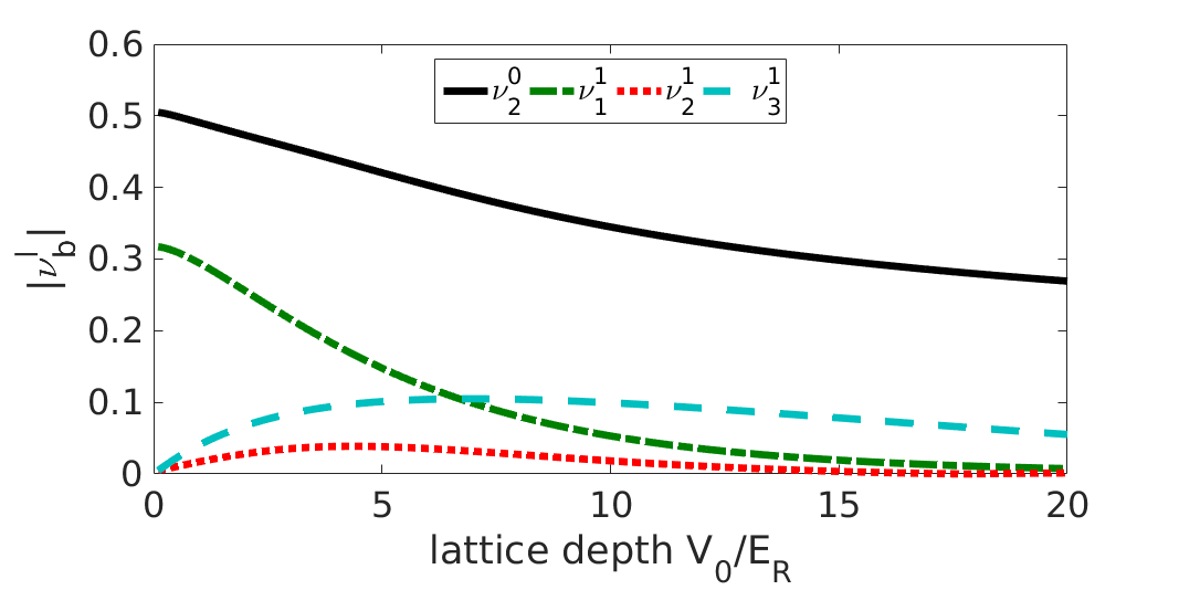
Figure 4: Coupling matrix elements $\nu^{\ell}_{b}=W_{b0}^{(\ell)}$ as defined in Eq. (29) for a static lattice of depth $V_{0}/E_{R}$.

In order to be explicit, in the following we will focus on transitions from the lowest to the second excited band. For small quasimomenta $k\ll\pi/a$ these transitions constitute the dominant heating channel. The relevant matrix element $W_{20}^{(0)}$ has a rather weak dependence on the lattice depth, as can be seen from Fig. 4 where this parameter is plotted for a lattice of static depth $V_{0}$. Thus, when the lattice depth is modulated, $V_{0}\to V_{0}[1+\alpha\sin(\omega t)]$, we can approximate

$$W_{20}^{(0)}(t)\approx W-\alpha W^{\prime}\sin(\omega t),$$ (35)

neglecting higher harmonics. Both coefficients $W$ and $W^{\prime}$ have a very weak dependence on $\alpha$ only and one has $W^{\prime}\ll W\sim 1$. At an $n$“photon” resonance, we can likewise approximate the instantaneous energy difference between both bands like

$$E_{2}(q,t)-E_{0}(q,t)\approx\Delta(q)+\alpha F(q)\sin(\omega t)$$ (36)

and its inverse like

$$\frac{1}{E_{2}(q,t)-E_{0}(q,t)}\approx\frac{1}{\Delta(q)}-\alpha\frac{F(q)}{\Delta^{2}(q)}\sin(\omega t).$$ (37)

Taking terms up to $\alpha^{2}$, the matrix element $M_{20}(q,t)$ then reads

$$M_{20}(q,t)\approx-i\frac{V_{0}}{n}\big{[}\alpha W\cos(\omega t)-\alpha^{2}X(q)\sin(2\omega t)\big{]},$$ (38)

where we have used $\sin(a)\cos(a)=\sin(2a)/2$, employed the resonance condition

$$\Delta(q)=n\hbar\omega,$$ (39)

and defined

$$X(q)=\frac{1}{2}\bigg{[}W^{\prime}+\frac{F(q)}{\Delta(q)}\bigg{]},$$ (40)

where $X(q)\ll W$.

At the resonance $(2,n)$, we will describe the system within the the subspace spanned by the bands $b=0$ and $b=2$. Up to a time-dependent energy constant, the relevant Hamiltonian is given by

$$\hat{H}^{\prime}(q,t) \approx \big{[}n\hbar\omega+\alpha F(q)\sin(\omega t)\big{]}|2q\rangle\langle 2q|$$

$$+\,M_{20}(q,t)|2q\rangle\langle 0q|+M_{20}^{*}(q,t)|0q\rangle\langle 2q|.$$

The Fourier decomposition of the Hamiltonian is given by

$$\hat{H}^{\prime}(q,t) = \sum_{m}\hat{H}^{\prime}_{m}(q)e^{im\omega t},$$ (42)

$$\hat{H}^{\prime}_{m}(q) = \frac{1}{T}\int_{0}^{T}\!\mathrm{d}t\,e^{-im\omega t}\hat{H}^{\prime}(q,t),$$ (43)

with driving period $T=2\pi/\omega$, we find

$$\hat{H}^{\prime}_{0}(q) = n\hbar\omega|2q\rangle\langle 2q|,$$ (44)

$$\hat{H}^{\prime}_{1}(q) = -i\frac{\alpha F(q)}{2}|2q\rangle\langle 2q|$$ (46)

$$-i\,\frac{\alpha V_{0}W}{2n}\big{(}|2q\rangle\langle 0q|-|0q\rangle\langle 2q|\big{)},$$

$$\hat{H}^{\prime}_{2}(q) = \frac{\alpha^{2}V_{0}X(q)}{2n}\big{(}|2q\rangle\langle 0q|-|0q\rangle\langle 2q|\big{)},$$ (47)

as well as the conjugated terms $\hat{H}_{-m}=\hat{H}_{m}^{\dagger}$. The terms $\hat{H}_{m}$ become smaller with increasing $m$ and depend on the driving strength like $\alpha^{|m|}$. This applies also to the higher harmonics that we neglected.

IV.2 Rotating-wave approximation

If the coupling matrix element $M_{20}(q,t)$ is small compared to the driving frequency $\hbar\omega$ (both scale like $1/n$), a rotating wave approximation is justified. For this approximation, we perform yet another gauge transformation, with the unitary operator

$$\hat{U}^{\prime}(t)=\exp\Big{(}-i\sum_{q}\Big{[}n\omega t-\frac{\alpha F(q)}{\hbar\omega}\cos(\omega t)\Big{]}|2q\rangle\langle 2q|\Big{)}.$$ (48)

Assuming the resonance condition $(\ref{eq:resonance})$, the transformed Hamiltonian reads

$$\hat{H}^{\prime\prime}(q,t)=M_{20}(q,t)e^{in\omega t-i\frac{\alpha F(q)}{\hbar\omega}\cos(\omega t)}|2q\rangle\langle 0q|+\text{ h.c. }.$$ (49)

In the following, we will again drop the label $q$. Employing the relation

$$\exp(-ia\cos(b))=\sum_{k=-\infty}^{\infty}(-i)^{k}\mathcal{J}_{k}(a)e^{-ikb},$$ (50)

where $\mathcal{J}_{k}(x)$ denotes a Bessel function of the first kind, we find the Fourier components of the time-dependent matrix element

$$M_{20}(q,t)e^{in\omega t-i\frac{\alpha F(q)}{\hbar\omega}\cos(\omega t)}=\sum_{r}M^{(n)}_{r}e^{ir\omega t}$$ (51)

to be given by

$$M^{(n)}_{r} = -i\frac{\alpha V_{0}W}{2n}(-i)^{n+1-r}\mathcal{J}_{n+1-r}\big{(}{\textstyle\frac{\alpha F}{\hbar\omega}}\big{)}$$

$$\quad\,-i\frac{\alpha V_{0}W}{2n}(-i)^{n-1-r}\mathcal{J}_{n-1-r}\big{(}{\textstyle\frac{\alpha F}{\hbar\omega}}\big{)}$$

$$+\,\frac{\alpha^{2}V_{0}X}{2n}(-i)^{n+2-r}\mathcal{J}_{n+2-r}\big{(}{\textstyle\frac{\alpha F}{\hbar\omega}}\big{)}$$

$$-\,\frac{\alpha^{2}V_{0}X}{2n}(-i)^{n-2-r}\mathcal{J}_{n-2-r}\big{(}{\textstyle\frac{\alpha F}{\hbar\omega}}\big{)}.$$

For the rotating-wave approximation, we now neglect the rapidly rotating phases of the coupling matrix element,

$$M_{20}(q,t)e^{in\omega t-i\frac{\alpha F(q)}{\hbar\omega}\cos(\omega t)}\approx M^{(n)}_{0}.$$ (53)

The effective coupling parameter is, thus, given by

$$C_{(2,n)}=|M^{(n)}_{0}|.$$ (54)

In order to interpret this result, it is useful to make further approximations. First of all, let us consider only the leading order with respect to the driving strength $\alpha$. For this purpose, we note that for small arguments $x$ (and $k\geq 0$) the Bessel function is asymptotically given by

$$\mathcal{J}_{k}(x)\simeq\frac{1}{k!}\Big{(}\frac{x}{2}\Big{)}^{k}.$$ (55)

Hence, in leading order only the second and the fourth line of Eq. (IV.2) contribute to $M_{0}$ and we have

$$M^{(n)}_{0}\simeq(-i)^{n}\frac{\alpha V_{0}}{n}\bigg{[}\frac{W}{2}+\frac{(n-1)X\hbar\omega}{F}\bigg{]}\frac{\Big{(}\frac{\alpha F}{2\hbar\omega}\Big{)}^{\!n-1}}{(n-1)!}$$ (56)

For large “photon” numbers $n$, we can now use Stirling’s formula

$$k!\simeq\sqrt{2\pi k}\Big{(}\frac{k}{e}\Big{)}^{k}$$ (57)

valid for large $k$. We obtain

$$C_{(2,n)}\simeq\alpha V_{0}\sqrt{\frac{\pi}{2n^{3}}}\bigg{(}W+\frac{W^{\prime}\Delta}{F}+1\bigg{)}\bigg{(}\frac{\alpha}{\alpha_{\text{thresh}}}\bigg{)}^{\!n-1},$$ (58)

with the threshold value

$$\alpha_{\text{thresh}}=\frac{2\Delta}{eF}$$ (59)

for the driving strength. Here we also employed Eqs. (39) and (40). We can compare the estimate given by the rotating wave approximation to the numerical computed dynamics.

From the evolution shown in Fig. 3(a), we can extract the period $T^{\text{sim}}_{(2,2)}\approx 2.56\,\mathrm{ms}$ for $\alpha=0.3$, $\hbar\omega=3.9E_{R}$, $q=0$, $V_{0}/E_{R}=10$ and $E_{R}=3.33\cdot 2\pi\hbar\mathrm{kHz}$. For these parameters, we obtain $\Delta\approx 7.77E_{R}$, $F(0)\approx 5.51E_{R}$, $W\approx 0.345$, as well as $W^{\prime}\approx 0.12$. Using Eq. 14 and the rotating wave approximation for the coupling parameter (56) and (54), we obtain the estimate $T^{\text{RW}}_{(2,2)}\approx 2.03\,\mathrm{ms}$ for the oscillation period, which lies about twenty percent below the numerically observe value.

Equation (58) tells us that for large $n$ the onset of heating occurs in a rather sharp transition when the driving strength reaches the threshold. Namely, for $\alpha<\alpha_{\text{thresh}}$ the coupling parameter is exponentially suppressed with respect to $n=\Delta/\hbar\omega$. This result is favorable for Floquet engineering, as it tells us that for sufficiently low frequencies and not too strong driving, interband heating becomes very small. However, the predicted threshold is only valid as long as $M_{20}(t)$ is small compared to $\hbar\omega$ for $\alpha=\alpha_{\text{thresh}}$. If this is not the case, we have to go beyond the rotating wave approximation. This can be done using degenerate perturbation theory in Floquet space.

IV.3 Floquet perturbation theory

Let us now estimate the effective coupling parameter $C_{(2,n)}(q)$ for the resonant $n$-“photon” coupling of the states $|0q\rangle$ and $|2q\rangle$ using degenerate perturbation theory within the Floquet space of the driven system (see, e.g., Ref. Eckardt and Anisimovas (2015)). Within this space the state $|bq\rangle$ is represented by a family of states $|bqm\rangle\!\rangle$ labeled by an integer index $m$ that represent a time-dependent state in the original state space $|bq\rangle e^{im\omega t}$. The coupling between these states, which form a complete basis, is described by the quasienergy operator $\bar{Q}$ playing the role of a static Hamiltonian. Starting from the problem defined by the Hamiltonian $\hat{H}^{\prime}(q,t)$, the matrix matrix elements of the quasienergy operator are given by

$$\langle\!\langle b^{\prime}q^{\prime}m^{\prime}|\bar{Q}|bqm\rangle\!\rangle=\langle b^{\prime}q^{\prime}|(\delta_{m^{\prime}m}m\hbar\omega+\hat{H}^{\prime}_{m^{\prime}-m}(q))|bq\rangle,$$ (60)

where $\hat{H}^{\prime}_{m}(q)$ denote the Fourier components of the Hamiltonian. The eigenstates and eigenvalues of the quasienergy operator correspond to the time-periodic Floquet modes and their quasienergies, respectively, which play a role similar to that of the stationary states in undriven systems and their energies.

The integer $m$ plays the role of the relative occupation of a photonic mode in the classical limit of large occupation. In this interpretation the state $|bqm\rangle\!\rangle$ represents a product state $|bq\rangle|m\rangle$ solving the unperturbed problem

$$\langle\!\langle bqm^{\prime}|\bar{Q}_{0}|bqm\rangle\!\rangle = \delta_{m^{\prime}m}\langle b^{\prime}q^{\prime}|(m\hbar\omega+\hat{H}_{0}^{\prime})|bq\rangle$$

$$= \delta_{m^{\prime}m}\delta_{q^{\prime}q}\delta_{b^{\prime}b}\big{[}m\hbar\omega+\varepsilon_{b}(q)\big{]}.$$

The unperturbed quasienergy $\varepsilon_{bm}(q)$ is thus given by the “photonic” energy $m\hbar\omega$ plus the system energy

$$\frac{1}{T}\varepsilon_{b}(q)=\int_{0}^{T}\!\mathrm{d}t\,E_{b}(q,t),$$ (62)

$\varepsilon_{bm}(q)=m\hbar\omega+\varepsilon_{b}(q)$. The coupling between the “photonic” mode and the system is described by the Fourier components $\hat{H}_{m}$ of the Hamiltonian with $m\neq 0$,

$$\langle\!\langle bqm^{\prime}|\bar{V}|bqm\rangle\!\rangle = \langle\!\langle bqm^{\prime}|(\bar{Q}-\bar{Q}_{0})|bqm\rangle\!\rangle$$

$$= (1-\delta_{m^{\prime}m})\delta_{q^{\prime}q}\langle b^{\prime}q|\hat{H}_{m^{\prime}-m}(q)|bq\rangle.$$

In order to describe the coupling between the lowest and the second excited band, let us write down the relevant matrix elements of the quasienergy operator explicitly. For the sake of a light notation, we will again suppress the label $q$. The diagonal matrix elements are given by

$$\langle\!\langle 0m|\bar{Q}_{0}|0m\rangle\!\rangle = m\hbar\omega,$$ (64)

$$\langle\!\langle 2m|\bar{Q}_{0}|2m\rangle\!\rangle = m\hbar\omega+\varepsilon_{2},$$ (65)

where $\varepsilon_{0}=0$ was chosen for convenience. At the $n$-“photon” resonance $(2,n)$, where the lowest band is resonantly coupled to the second excited band, we have

$$\varepsilon_{2}\approx n\hbar\omega,$$ (66)

so that the states $|0m\rangle\!\rangle$ and $|2(m-n)\rangle\!\rangle$ are (nearly) degenerate. The relevant coupling matrix elements of the perturbation $\bar{V}$ change the photon number $m$ by $\pm 1$ or by $\pm 2$ (so that for $n>2$ necessarily higher-order processes have to be taken into account in order to describe the coupling between $|0m\rangle\!\rangle$ and $|2(m-n)\rangle\!\rangle$). They are given by

$$\langle\!\langle 2(m\pm 1)|\bar{V}|2m\rangle\!\rangle = \mp i\frac{\alpha F}{2}$$ (67)

$$\langle\!\langle 2(m\pm 1)|\bar{V}|0m\rangle\!\rangle = -i\frac{\alpha V_{0}W}{2n}$$ (68)

$$\langle\!\langle 2(m\pm 2)|\bar{V}|0m\rangle\!\rangle = \pm\frac{\alpha^{2}V_{0}X}{2n}$$ (69)

and the hermitian conjugated terms, where we have employed Eqs. (46) and (47).

The coupling parameter $C_{(b,n)}$ introduced in Eq. (14) corresponds to the absolute value of the matrix element coupling the states $|0m\rangle\!\rangle$ and $|2(m-n)\rangle\!\rangle$ in Floquet space. For the single-“photon” resonance with $n=1$, both states are directly coupled by the matrix element (68), so that the coupling parameter reads

$$C_{(2,1)}=|\langle\!\langle 2(m-1)|\bar{V}|0m\rangle\!\rangle|=\frac{\alpha V_{0}W}{2}.$$ (70)

For the two-“photon” resonance with $n=2$, we have two relevant contributions to the coupling parameter,

$$C_{(2,2)}=\big{|}C^{(1)}_{(2,2)}+C^{(2)}_{(2,2)}\big{|}.$$ (71)

The first contribution directly corresponds to the matrix element (69) describing a two-photon process,

$$C^{(1)}_{(2,2)}=\langle\!\langle 2(m-2)|\bar{V}|0m\rangle\!\rangle=-\frac{\alpha^{2}V_{0}X}{4}.$$ (72)

The second contribution stems from the second-order processes $|0m\rangle\!\rangle\to|2(m-1)\rangle\!\rangle\to|2(m-2)\rangle\!\rangle$, where both states are coupled via an energetically distant intermediate state. The unperturbed quasienergy of this intermediate state, $\varepsilon_{2(m-1)}=n\hbar\omega+(m-1)\hbar\omega$, lies $\hbar\omega$ above the quasienergy $\varepsilon_{0m}=\varepsilon_{2(m-n)}=m\hbar\omega$ of the degenerate doublet. According to the rules of degenerate perturbation theory (see, e.g., Ref. Eckardt and Anisimovas (2015)), we find

$$C^{(2)}_{(2,2)} = \frac{\langle\!\langle 2(m-2)|\bar{V}|2(m-1)\rangle\!\rangle\langle\!\langle 2(m-1)|\bar{V}|0m\rangle\!\rangle}{\varepsilon_{0m}-\varepsilon_{2(m-1)}}$$

$$= -\frac{\alpha^{2}FV_{0}W}{8\hbar\omega}.$$

Let us finally have a closer look also at the three “photon” process with $n=3$. The coupling parameter is a combination of three contributions,

$$C_{(2,3)}=\big{|}C^{(2)}_{(2,3)}+C^{(3a)}_{(2,3)}+C^{(3b)}_{(2,3)}\big{|}.$$ (74)

The first contribution stems from the second-order process $|0m\rangle\!\rangle\to|2(m-2)\rangle\!\rangle\to|2(m-3)\rangle\!\rangle$. The intermediate state has a quasienergy lying $\hbar\omega$ above the degenerate doublet and the resulting coupling is given by

$$C^{(2)}_{(2,3)} = \frac{\langle\!\langle 2(m-3)|\bar{V}|2(m-2)\rangle\!\rangle\langle\!\langle 2(m-2)|\bar{V}|0m\rangle\!\rangle}{\varepsilon_{0m}-\varepsilon_{2(m-2)}}$$

$$= -\frac{\alpha^{3}FV_{0}X}{4n\hbar\omega}.$$

The second contribution stems from the third-order processes $|0m\rangle\!\rangle\to|2(m-1)\rangle\!\rangle\to|0(m-1)\rangle\to|2(m-3)\rangle\!\rangle$. The quasienergies of both intermediate states are separated by $2\hbar\omega$ and $-\hbar\omega$ from the degenerate doublet of states to be coupled. The matrix element is, thus, of the order of

$$C^{(3a)}_{(2,3)}\sim\bigg{(}-i\frac{\alpha V_{0}W}{2n}\bigg{)}^{3}\frac{1}{(-2\hbar\omega)(\hbar\omega)}=-i\frac{\alpha^{3}V_{0}^{3}W^{3}}{432(\hbar\omega)^{2}}.$$ (76)

The third contribution stems, finally, from the third order process $|0m\rangle\!\rangle\to|2(m-1)\rangle\!\rangle\to|2(m-2)\rangle\to|2(m-3)\rangle\!\rangle$. The quasienergies of both intermediate states are separated by $2\hbar\omega$ and $\hbar\omega$ from the degenerate doublet. The corresponding coupling parameter is of the order of

$$C^{(3b)}_{(2,3)}\sim\bigg{(}\frac{i\alpha F}{2}\bigg{)}^{2}\frac{-i\alpha V_{0}W}{2n}\frac{1}{(-2\hbar\omega)(-\hbar\omega)}=i\frac{\alpha^{3}F^{2}V_{0}W}{32(\hbar\omega)^{2}}.$$ (77)

Extending the perturbative arguments used here to higher orders of the perturbation theory, one can estimate also the coupling parameters $C_{(2,n)}$ for multi-“photon” transitions with $n>3$. A similar approach can, moreover, also be applied for transitions to the first excited band or higher lying bands. In leading order in the driving strengths $\alpha$, we can again cast the coupling parameters into the very same form

$$C_{(b,n)}=\alpha B_{(b,n)}\bigg{(}\frac{\alpha}{\alpha_{(b,n)}}\bigg{)}^{\!n-1}$$ (78)

encountered already within the rotating-wave approximation (58), with energy scale $B_{(b,n)}$ and threshold driving strength $\alpha_{(b,n)}$. This form implies that for below-threshold driving, $\alpha<\alpha_{(b,n)}$, interband excitation processes are suppressed exponentially for large “photon” numbers $n=\Delta/(\hbar\omega)$, that is for low frequencies. However, while Eq. (78) is of the same form as the rotating-wave result, the coefficient $B_{(b,n)}$ and the threshold value $\alpha_{(b,n)}$ will generally be different.

The characteristic driving strength $\alpha_{(b,n)}$, below which heating is suppressed, might show oscillatory behavior between even and odd $n$. Apart from such details, let us estimate how $\alpha_{(b,n)}$ scales when $n$ becomes large. For that purpose, the first quantity to be studied are the energy denominators of the perturbatively computed coupling parameters. They are given by the product of the quasienergies that the intermediate states have with respect to the degenerate doublet of states to be coupled. Taking, for simplicity, a sequence of processes that lower the “photon” number in steps of one, these denominators provide a factor of

$$\frac{1}{(n-1)!(\hbar\omega)^{n-1}}\simeq\frac{1}{\sqrt{2\pi(n-1)}}\bigg{(}\frac{e}{(n-1)\hbar\omega}\bigg{)}^{(n-1)},$$ (79)

where we have again used Stirling’s formula (57). This result indicates that the energy denominators contribute a factor of $n\hbar\omega/e=\Delta/e$ to $\alpha_{(b,n)}$, which for fixed $\Delta$ is independent of $n$. Similar results are obtained for sequences involving individual processes that lower the “photon” number in steps larger than one. Apart from the energy denominators also the matrix elements contribute to $\alpha_{(b,n)}$. In the present example of a lattice with modulated lattice depth, we must expect that the $1/n$-dependence of the matrix elements (68) and (69) leads to an increase of $\alpha_{(b,n)}$ with $n$. This effect is not captured by the rotating-wave approximation, which takes these matrix elements into account in linear order only. It can explain the behavior visible in Fig. 2 that for lower driving frequencies larger driving strengths are required for significant resonant excitation.

We have started our perturbation expansion from the Hamiltonian $\hat{H}^{\prime}(q,t)$ given by Eq. (IV.1). In order to systematically improve the result (58) obtained within the rotating wave approximation, one can also start from the transformed Hamiltonian $\hat{H}^{\prime\prime}(q,t)$ given by Eq. (49). In this case we would recover the result (54) already in first order. Note that the coupling matrix element (54) contains infinite powers of the matrix element (67), while it is linear in the matrix elements (68) and (69). Transforming from $\hat{H}^{\prime}(q,t)$ to $\hat{H}^{\prime\prime}(q,t)$, thus, corresponds to a resummation of part of the perturbation series obtained for $\hat{H}^{\prime}(q,t)$ to infinite order.

V Conclusions

We investigated limitations of the low-frequency approximation that underlies typical protocols of Floquet engineering in systems of ultracold atomic quantum gases in driven optical lattices. We stressed that already single-particle processes can lead to unwanted transfer to excited orbital states beyond the low-frequency approximation. In order to illustrate this fact, we studied the example of a one-dimensional optical lattice driven by a modulation of the lattice depth. For that purpose we combined two different approaches. On the one hand, we computed excitation spectra of the driven system by numerical means. On the other hand, we estimated the effective coupling parameters for resonant interband transitions using an analytical approach involving perturbation theory in Floquet space. The latter approach is able to explain important features of the numerically computed spectra, like a momentum-dependent suppression of transitions to the first excited band. The most important result is, however, the prediction of a threshold value of the driving strength, below which interband excitations are suppressed exponentially for large $n$, that is for large inverse driving frequencies.

We expect that this exponential suppression of interband heating with $n$ for below-threshold driving is a rather general feature, which is found also for lattices driven by other forms of periodic forcing. Namely, the arguments that we employed to motivate the form (78) of the effective coupling matrix element $C_{b,n}$ for an $n$-“photon” interband excitation process are rather general.

One example for another driving scheme is the shaken optical lattice investigated in Ref. Weinberg et al. (2015). For this system the driving strength $K$ can be defined as the amplitude of the potential modulation between neighboring lattice sites in the comoving lattice frame, carrying the dimension of an energy. Using the above arguments together with the perturbation theory worked out in appendix of Ref. Weinberg et al. (2015), the threshold driving strength can be evaluated to read

$$K_{(1,n)}=\frac{2\eta_{10}\Delta}{e},$$ (80)

where $\eta_{01}$ is a dimensionless matrix element describing the coupling between the two lowest bands. However, in the shaken optical lattice the physics of the system is mainly determined by the scaled driving amplitude $K/(\hbar\omega)$. The threshold value for this relevant quantity grows linearly with the “photon” number, $[K/(\hbar\omega)]_{(1,n)}=\Delta/(e\hbar\omega)=n/e$.

We can now draw two conclusions concerning interband heating processes in Floquet driven optical lattices: On the one hand, heating processes to excited orbital states are a relevant heating channel in periodically driven optical lattices already on the single-particle level. On the other hand, such heating can be suppressed efficiently, provided that both (i) the driving frequency is low enough, so that heating corresponds to $n$-“photon” transitions with large $n\gg 1$, and (ii) the driving strength remains below the threshold value. Our results contribute to a theoretical foundation of Floquet engineering in periodically driven lattices.

Relevant questions to be addressed in future work concern interband heating rates induced by driving schemes that were used to Floquet engineer artificial gauge fields. This includes driving functions involving higher harmonics of the driving frequency, as they were used in the experiments described in Refs. Struck et al. (2012, 2013), as well as lattices that are driven by a moving running waves in order to create the Hofstadter Hamiltonian Aidelsburger et al. (2015, 2013); Miyake et al. (2013); Kennedy et al. (2015). Furthermore, it will be crucial to understand in how far such single-particle heating channels are modified in systems of interacting particles. Also heating induced by two-particle scattering processes deserves further investigation.