Direct Visual Odometry using Bit-Planes

Abstract

Feature descriptors, such as SIFT and ORB, are well-known for their robustness to illumination changes, which has made them popular for feature-based VSLAM. However, in degraded imaging conditions such as low light, low texture, blur and specular reflections, feature extraction is often unreliable. In contrast, direct VSLAM methods which estimate the camera pose by minimizing the photometric error using raw pixel intensities are often more robust to low textured environments and blur. Nonetheless, at the core of direct VSLAM is the reliance on a consistent photometric appearance across images, otherwise known as the brightness constancy assumption. Unfortunately, brightness constancy seldom holds in real world applications.

In this work, we overcome brightness constancy by incorporating feature descriptors into a direct visual odometry framework. This combination results in an efficient algorithm that combines the strength of both feature-based algorithms and direct methods. Namely, we achieve robustness to arbitrary photometric variations while operating in low-textured and poorly lit environments. Our approach utilizes an efficient binary descriptor, which we call Bit-Planes, and show how it can be used in the gradient-based optimization required by direct methods. Moreover, we show that the squared Euclidean distance between Bit-Planes is equivalent to the Hamming distance. Hence, the descriptor may be used in least squares optimization without sacrificing its photometric invariance. Finally, we present empirical results that demonstrate the robustness of the approach in poorly lit underground environments.

I Introduction

Visual Odometry (VO) is the problem of estimating the relative pose between cameras sharing a common field of view. Due to its importance, VO has received a large amount of attention in the literature as evident by the number of high quality systems freely available to the community [18, 42, 19, 21]. Current systems, however, are not equipped to tackle environments with challenging illumination conditions such as the ones shown in Figs. 1 and 2. In this paper, our goal is to enable vision-only pose estimation to operate robustly in such challenging environments.

Current state-of-the-art algorithms rely on a feature-based pipeline [52], where keypoint correspondences are used to obtain an estimate of the camera motion (e.g. [44, 42, 5, 38, 27, 31, 28, 20]). However, the performance of feature extraction and matching struggles under challenging imaging conditions, such as motion blur, low light, and repetitive texture [41, 50]. An example environment where keypoint extraction is not easily possible is shown in Fig. 1. If the feature-based pipeline fails, a vision-only system has little hope of recovery.

An alternative to the feature-based pipeline is the use of pixel intensities directly, or what is commonly referred to as direct methods [37, 30]. The use of direct methods has been recently popularized with the introduction of the Kinect as a real-time source for high-frame rate depth and RGB data [34, 33, 51, 23, 54] as well as monocular SLAM algorithms [18, 19]. When the apparent image motion is small, direct methods deliver more robustness and accuracy as the majority of pixels in the image could be used to estimate a small number of degrees-of-freedom as demonstrated by several authors [43, 12, 19, 49].

Nonetheless, as pointed out by other researchers [42], the main limitation of direct methods is their reliance on a consistent appearance between the matched pixels, otherwise known as the brightness constancy assumption [26, 22], which is seldom satisfied in real world applications.

Due to the complexity of real world illumination conditions, an efficient solution to the problem of appearance change for direct VO is challenging. The most common scheme to mitigating the effects of illumination change is to assume a parametric illumination model that is estimated alongside the camera pose, such as the gain and bias model [34, 17]. This approach is limited by definition and does not address the plethora of the possible non-global and nonlinear intensity deformations. More sophisticated techniques have been proposed [49, 36, 40], but either assume a certain structure of the scene (such as local planarity) thereby limiting applicability, heavily rely on dense depth estimates (which is not always possible), or significantly increase the dimensionality of the state vector and thereby the computational cost to account for a complex illumination model.

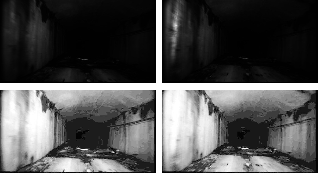
Figure 1: Shown at the top row are two consecutive images collected from an underground mine. The bottom row shows a histogram equalization of the images for better visualization. The equalized images may appear noiseless due to its smooth appearance in the document (due to resizing). The data has a low signal-to-noise ratio due to the poor illumination of the scene.

Figure 2: An example of the nonlinear intensity deformation caused by the automatic camera settings. A common problem with outdoor applications of robot vision.

I-A Contributions

In this work, we relax the photometric consistency assumption required by most direct VO algorithms thus allowing them to operate in environments where the appearance between images vary considerably. We achieve this by combining the illumination invariance afforded by feature descriptors within a direct alignment framework. This in fact is a challenging problem, as conventional illumination invariant feature descriptors are not well-suited to the iterative gradient-based optimization at the heart of direct methods. Our contributions in this work are as follows:

• We combine descriptors from feature-based methods within a direct alignment framework to allow vision-only pose estimation in challenging environments where the current state-of-the-art in feature-based, and direct VSLAM provide unsatisfactory results.

• We introduce a binary descriptor [3], show how it can be integrated into a direct method and demonstrate its suitability for linearization. Moreover, we show that under a least squares cost functions the method is equivalent to the Hamming distance over the binary descriptor space. We call this descriptor Bit-Planes.

• We have previously developed Bit-Planes and demonstrated its performance on template tracking under challenging illumination conditions [3]. In this work, we demonstrate the effectiveness of the descriptor on the more challenging task of VO from relatively sparse and noisy depth measurements.

• We show that the approach is efficient and robust using a combination of synthetic and real data to evaluate performance as compared to existing method.

Figure 3: Local intensity comparisons in a $3\times 3$ neighborhood. In LABEL:fig:ct1 the center pixel is highlighted, and compared to its neighbors as shown in LABEL:fig:ct2. The descriptor is obtained by combining the results of each comparison in LABEL:fig:ct3 into a single scalar descriptor [45, 55].

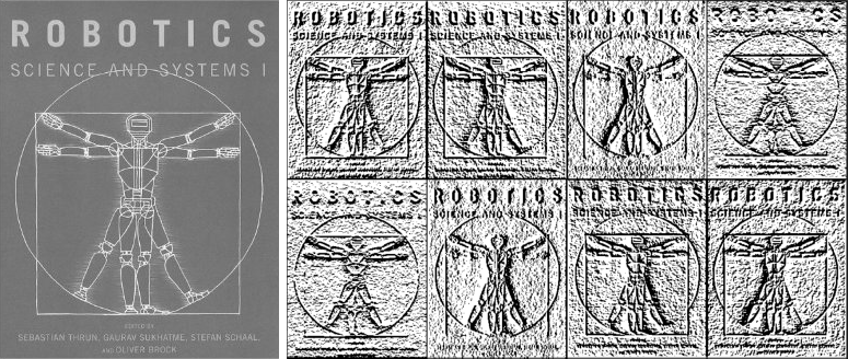
Figure 4: An illustration of our Bit-Planes descriptor where each channel is composed of bits. Since the residual vector is binary, least squares minimization becomes equivalent to minimizing the Hamming distance.

II Background

II-A Direct Visual Odometry

Let the intensity, and depth of a pixel coordinate $\mathbf{p}={\left(x,~{}y\right)}^{\mathstrut\scriptscriptstyle{\top}}$ at the reference image be respectively given by $\mathbf{I}(\mathbf{p})\in\mathbb{R}$ and $\mathbf{D}(\mathbf{p})\in\mathbb{R}^{+}$. Upon a rigid-body motion of the camera a new image is obtained $\mathbf{I}^{\prime}(\mathbf{p}^{\prime})$. The goal of conventional direct VO is to estimate an increment of the camera motion parameters $\Delta\bm{\theta}\in\mathbb{R}^{6}$ such that the photometric error is minimized

$$\Delta\bm{\theta}^{\ast}=\underset{\Delta\bm{\theta}}{\operatorname*{argmin}}{\sum_{\mathbf{p}\in\Omega}{\left\|{\mathbf{I}^{\prime}\left(\mathbf{w}(\mathbf{p};\bm{\theta}+\Delta\bm{\theta})\right)-\mathbf{I}\left(\mathbf{p}\right)}\right\|}^{2}},$$ (1)

where $\Omega$ is a subset of pixel coordinates of interest in the reference frame, $\mathbf{w}\left(\cdot\right)$ is a warping function that depends on the parameter vector we seek to estimate, and $\bm{\theta}$ is an initial estimate. After every iteration, the current estimate of parameters is updated additively (i.e. $\bm{\theta}\leftarrow\bm{\theta}+\Delta\bm{\theta}$). The process repeats until convergence, or some termination criteria have been met. This is the well known Lucas and Kanade (forward additive) algorithm [37].

By (conceptually) interchanging the roles of the template and input images, Baker & Matthews’ devise a more efficient alignment techniques known as the Inverse Compositional (IC) algorithm [6]. Under the IC formulation we seek an update $\Delta\bm{\theta}$ that satisfies

$${\Delta\bm{\theta}}^{\ast}=\underset{\Delta\bm{\theta}}{\operatorname*{argmin}}{\sum_{\mathbf{p}\in\omega}{\lVert\mathbf{I}\left(\mathbf{w}(\mathbf{p};\Delta\bm{\theta})\right)-\mathbf{I}^{\prime}\left(\mathbf{w}(\mathbf{p};\bm{\theta})\right)\rVert^{2}}}.$$ (2)

The optimization problem in Eq. 2 is nonlinear irrespective of the form of the warping function or the parameters, as in general there is no linear relationship between pixel coordinates and their intensities. By equating the partial derivatives of the first-order Taylor expansion of Eq. 2 to zero, we reach at solution given by the following closed-form (normal equations)

$$\Delta\bm{\theta}={\left({\mathbf{J}}^{\mathstrut\scriptscriptstyle{\top}}{\mathbf{J}}\right)}^{-1}{\mathbf{J}}^{\mathstrut\scriptscriptstyle{\top}}\mathbf{e},$$ (3)

where $\mathbf{J}=\left({\mathbf{g}(\mathbf{p}_{1})}^{\mathstrut\scriptscriptstyle{\top}},~{}\ldots,~{}{\mathbf{g}(\mathbf{p}_{m})}^{\mathstrut\scriptscriptstyle{\top}}\right)\in\mathbb{R}^{m\times p}$ is the matrix of first-order partial derivatives of the objective function, or the Jacobian, $m$ is the number of pixels, and $p=\left|\bm{\theta}\right|$ is the number of parameters. Each $\mathbf{g}$ is $\in\mathbb{R}^{1\times p}$ and is given by the chain rule as

$$\mathbf{g}(\mathbf{p})^{\mathstrut\scriptscriptstyle{\top}}=\nabla\mathbf{I}(\mathbf{p})\frac{\partial\mathbf{w}}{\partial\bm{\theta}},$$ (4)

where $\nabla\mathbf{I}=\left(I_{x},~{}I_{y}\right)\in\mathbb{R}^{1\times 2}$ is the image gradient along the $x$- and $y$- directions respectively. Finally,

$$\mathbf{e}(\mathbf{p})=\mathbf{I}^{\prime}(\mathbf{w}(\mathbf{p};\bm{\theta}))-\mathbf{I}(\mathbf{p})$$ (5)

is the vector of residuals, or the error image. Parameters of the motion model are updated via the IC rule given by

$$\mathbf{w}\left(\mathbf{p},\bm{\theta}\right)\leftarrow\mathbf{w}\left(\mathbf{p},\bm{\theta}\right)\circ{\mathbf{w}\left(\mathbf{p},\Delta\bm{\theta}\right)}^{-1}.$$ (6)

We refer the reader to the excellent series by Baker and Matthews [6] for a detailed treatment.

II-B Image Warping

Given a rigid body motion $\mathbf{T}(\bm{\theta})\in SE(3)$ and a depth value $\mathbf{D}(\mathbf{p})$ in the coordinate frame of the template image, warping to the coordinate frame of the input image is performed according to

$$\mathbf{p}^{\prime}=\pi\left(\mathbf{T}(\bm{\theta})\pi^{-1}(\mathbf{D}(\mathbf{p})\right),$$ (7)

where $\pi\left(\cdot\right):\mathbb{R}^{3}\rightarrow\mathbb{R}^{2}$ denotes the projection onto a camera with a known intrinsic calibration, and $\pi^{-1}\left(\cdot,\cdot\right):\mathbb{R}^{2}\times\mathbb{R}\rightarrow\mathbb{R}^{3}$ denotes the inverse of this projection given the camera intrinsics and the pixel’s depth. Finally, the intensity values corresponding to the warped input image $\mathbf{I}(\mathbf{p}^{\prime})$ are obtained via a suitable interpolation scheme (bi-linear in this work).

III Binary Descriptor Constancy Direct VO

A limitation of direct method is the reliance on the brightness constancy assumption (Eq. 1). To circumvent this shortcoming, we propose the use of a descriptor constancy assumption. Namely, we seek an update to the pose parameters such that

$$\Delta\bm{\theta}^{\ast}=\underset{\Delta\bm{\theta}}{\operatorname*{argmin}}{{\left\|{\bm{\phi}(\mathbf{I}^{\prime}\left(\mathbf{w}(\mathbf{p};\bm{\theta}+\Delta\bm{\theta})\right))-\bm{\phi}(\mathbf{I}\left(\mathbf{p}\right))}\right\|}^{2}},$$ (8)

where $\bm{\phi(\cdot)}$ is a feature descriptor such as SIFT [35], HOG [14], or ORB [47]. The idea of using descriptors in lieu of intensity has been recently explored in optical flow estimation [48], template tracking [3], image-based tracking of a known 3D model [13], Active Appearance Models [4], and inter-object category alignment [10], in which results are very encouraging and consistently outperform classical minimization of the photometric error. To date, however, the idea has not been explored in the context of real-time direct VO with relatively sparse and noisy depth estimates.

The descriptor constancy objective in Eq. 8 is more complicated than its brightness counterpart in Eq. 1 as interesting feature descriptors are high dimensional and the suitability of their linearization remains unclear, and is only beginning to be investigated in the literature [4, 10].

In VO, however, another challenge is the need for an efficient feature descriptor suitable for real-time implementation. Densely computing classical descriptors such as HOG [14] and SIFT [35] becomes infeasible for real-time performance with a limited computational budget. Simpler descriptors, such as photometrically normalized image patches, or the gradient-constraint [11], are efficient to compute, but do not possess sufficient invariance to radiometric changes in the wild. Additionally, since reliable depth estimates from stereo are sparse, warping feature descriptors is challenging as it harder to reason about visibility and occlusions from sparse 3D points.

In this work, we propose a novel descriptor that satisfies the requirements for efficient direct alignment under challenging illumination, we also show its suitability for VO from relatively sparse depth data. Namely, our descriptor has the following properties:

• Invariance to monotonic changes in intensity, which is important as many robotic applications rely on automatic camera gain and exposure control. Gain adjustment (gamma correction) such as the one shown in Fig. 2 results in nonlinear changes in image appearance that are not captured by additive, or multiplicative terms.

• Computational efficiency, even on embedded devices, which is required for real-time VO, and

• Suitability for least squares minimization (e.g. Eq. 8). This is important for two reasons. First, solutions to least squares problems are the among the most computationally efficient optimization problems with a plethora of ready to use software packages. Second, due to the small residuals nature of least squares, only first-order derivatives are required to compute a good approximation of the Hessian. Hence, increasing efficiency and avoiding numerical errors associated with estimating second-order derivatives that arise, for example, when using alignment algorithms based on intrinsically robust objectives [16, 29, 15].

III-A The Bit-Planes Descriptor

The rationale behind binary descriptors is that using relative changes of pixel intensities is more robust than working with the raw values for correspondence estimation tasks. As with all binary descriptors, we perform local comparisons between the pixel and its immediate neighbors as shown in Fig. 3. We found that a $3\times 3$ neighborhood is sufficient when working with high-frame rate data and is the most efficient to compute. This is step is identical to the Census Transform [55], also known as LBP [45]. Choice of the comparison operator is arbitrary and will be denoted with $\bowtie\in\{>,\geq,<,\leq\}$. Since the binary representation of the descriptor requires eight comparisons in a $3\times 3$ neighborhood, it is commonly compactly stored as a single byte according to

$$\bm{\phi}_{\textsc{byte}}(\mathbf{x})=\sum_{i=1}^{8}2^{i-1}\big{[}\mathbf{I}(\mathbf{x})\bowtie\mathbf{I}(\mathbf{x}+\Delta\mathbf{x}_{i})\big{]},$$ (9)

where ${\{\Delta\mathbf{x}_{i}\}}_{i=1}^{8}$ is the set of the eight relative coordinate displacements that are possible within a $3\times 3$ neighborhood around the center pixel location $\mathbf{x}$.

In order for the descriptor to maintain its morphological invariance to intensity changes it must be matched under a binary norm, such as the Hamming distance. The reason for this is easy to illustrate with an example. Consider two bit patterns differing at a single bit — which so happens to be at the most significant position —

$$\mathbf{a} =\left\{\mathtt{{\color[rgb]{1,0,0}1},0,1,0,1,1,1,0}\right\},\text{ and}$$

$$\mathbf{b} =\left\{\mathtt{{\color[rgb]{1,0,0}0},0,1,0,1,1,1,0}\right\}.$$

The two bit-strings are clearly similar and their distance under the Hamming norm is $1$. However, if the decimal representation is used and matched under the squared Euclidean distance, their distance becomes $128^{2}=16384$, which does not capture their closeness in the descriptor space. Hence, using the descriptor in its decimal form is no longer invariant to monotonic intensity change. Nonetheless, it is not possible to use the Hamming distance in least squares optimization, and so it is usually approximated [53], but at the cost of reduced invariance.

In our proposed descriptor, we avoid the approximation of the Hamming distance and instead store each bit/coordinate of the descriptor as its own image, namely

$$\bm{\phi}_{\textsc{bp}}(\mathbf{x})=\begin{bmatrix}\mathbf{I}(\mathbf{x})\bowtie\mathbf{I}(\mathbf{x}+\Delta\mathbf{x}_{1})\\ \vdots\\ \mathbf{I}(\mathbf{x})\bowtie\mathbf{I}(\mathbf{x}+\Delta\mathbf{x}_{8})\end{bmatrix}\in\mathbb{R}^{8}\;.$$ (10)

Since each coordinate of the 8-vector descriptor is binary (as shown in Fig. 4), we call our descriptor “Bit-Planes.” Using this descriptor it is now possible to minimize an equivalent form of the Hamming distance using ordinary least squares.

III-B Bit-Planes implementation details

In order to reduce the sensitivity of the descriptor to noise, the image is smoothed with a Gaussian filter in a $3\times 3$ neighborhood ($\sigma=0.5$). The effect of this smoothing will be investigated in Section V. Since the operations involved in extracting the descriptor are simple and data parallel, they can be done efficiently with SIMD (Single Instruction Multiple Data) instructions [8, 24, 9]. A pseudo code of our implementation is shown in LABEL:code:simd.

Listing 1: Data parallel impelmentation, where src and dst indicate pointers to the source and destination images. The symbol load denotes loading the line of data into a SIMD register. With SSE2, for example, 16 pixels are processed at once. Similarly, for the set operator that fills the register with a single value. The comparision operator ’>’ along with the logical AND ’&’ and logical OR ’|’ are overloaded for SIMD types using the appropriate machine instructions.

⬇

c = set(src[0]);

dst = ((load(src[-stride-1] > c)) & 0x01) |

((load(src[-stride ] > c)) & 0x02) |

((load(src[-stride+1] > c)) & 0x04) |

((load(src[ +1] > c)) & 0x08) |

((load(src[ -1] > c)) & 0x10) |

((load(src[+stride-1] > c)) & 0x20) |

((load(src[+stride ] > c)) & 0x40) |

((load(src[+stride+1] > c)) & 0x80) ;

III-C Pre-computing descriptors for efficiency

Descriptor constancy as stated in Eq. 8 requires re-computing the descriptors after every iteration of image warping. In addition to the extra computational cost of repeated applications of the descriptor, it is difficult to warp individual pixel locations with sparse depth. An approximation to the descriptor constancy objective in Eq. 8 is to pre-compute the descriptors and minimize the following expression instead:

$$\min_{\Delta\bm{\theta}}\sum_{\mathbf{p}\in\Omega}{\sum_{i=1}^{8}{\lVert\bm{\Phi}^{\prime}_{i}(\mathbf{w}(\mathbf{p};\bm{\theta}+\Delta\bm{\theta}))-\bm{\Phi}_{i}(\mathbf{p})\rVert^{2}}},$$ (11)

where $\bm{\Phi}_{i}$ indicates the $i$-th coordinate of the pre-computed descriptor. We found that the loss of accuracy caused by using Eq. 11 instead of Eq. 8 to be insignificant in comparison to the computational savings.

IV VO using Bit-Planes

We will use Eq. 11 as our objective function, which we minimize using the Baker and Matthews’ IC formulation [6], allowing us to pre-compute the Jacobian of the cost function. The Jacobian is given by

$$\sum_{\mathbf{p}\in\Omega}\sum_{i=1}^{8}\mathbf{g}_{i}(\mathbf{p};\bm{\theta})^{\mathstrut\scriptscriptstyle{\top}}\mathbf{g}_{i}(\mathbf{p};\bm{\theta}),$$ (12)

where

$$\mathbf{g}_{i}(\mathbf{q};\bm{\theta})=\frac{\partial\bm{\Phi}_{i}}{\partial\mathbf{p}}\Bigr{\rvert}_{\mathbf{p}=\mathbf{q}}\frac{\partial\mathbf{w}}{\partial\bm{\theta}}\Bigr{\rvert}_{\mathbf{p}=\mathbf{q},\bm{\theta}=\mathbf{0}}\;\;.$$ (13)

Similar to other direct VO algorithms [32, 34, 1] pose parameters are represented with the exponential map, i.e. $\bm{\theta}=\left[\bm{\omega},~{}\bm{\nu}\right]^{\mathstrut\scriptscriptstyle{\top}}\in\mathbb{R}^{6}$. A rigid-body transformation $\mathbf{T}(\bm{\theta})\in SE(3)$ is obtained in closed-form for $\theta=\lVert\bm{\omega}\rVert\neq 0$, $s=\sin\theta$, and $\bar{c}=1-\cos\theta$ as

$$\exp\left(\bm{\theta}\right) =\begin{bmatrix}\mathbf{I}+s\left[\bm{\omega}\right]_{\times}+\bar{c}\left[\bm{\omega}\right]_{\times}^{2}&\mathbf{A}(\bm{\omega})\bm{\nu}\\ \mathbf{0}^{\mathstrut\scriptscriptstyle{\top}}&1\end{bmatrix}\;\in SE(3),$$ (14)

$$\mathbf{A}(\bm{\omega}) =\mathbf{I}+\frac{\bar{c}}{\theta}\left[\bm{\omega}\right]_{\times}+\frac{\theta-s}{\theta}\left[\bm{\omega}\right]_{\times}^{2}\;\in\mathbb{R}^{3\times 3}\;.$$ (15)

To improve the computational running time of the algorithm, we subsample pixel locations for use in direct VO. A pixel is selected for the optimization if its absolute gradient magnitude is non-zero and is a strict local maxima in a $3\times 3$ neighborhood. The intuition for this pixel selection procedure is that pixels with a small gradient magnitude contribute little, if any, to the objective function as the term in Eq. 13 vanishes. We compute the pixel saliency map for all eight Bit-Planes coordinate as

$$\mathbf{G}=\sum_{i=1}^{8}\sum_{\mathbf{p}}\left|\nabla_{x}\bm{\Phi}_{i}(\mathbf{p})\right|+\left|\nabla_{y}\bm{\Phi}_{i}(\mathbf{p})\right|.$$ (16)

An example of this saliency map is shown in Fig. 5. This pixel selection procedure is performed if the image resolution is at least $320\times 240$. For lower resolution images (coarser pyramid levels) we use all pixels with non-zero saliency without the non-maxima suppression step.

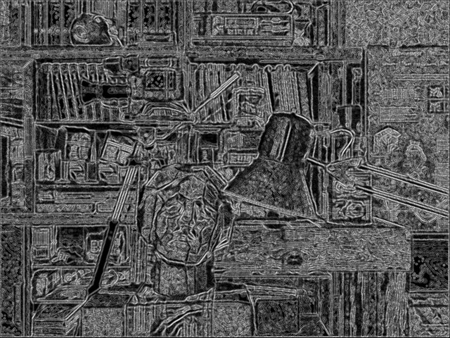
Figure 5: The absolute gradient magnitude of Bit-Planes over all channels. Darker values are smaller.

Minimization of the objective function is performed using an iteratively re-weighted Gauss-Newton algorithms. The weights are computed using the Tukey bi-weight function [7] given by

$$\rho(r_{i};\tau)=\begin{cases}{\left(1-{\left(r_{i}/\tau\right)}^{2}\right)}^{2}&\text{if }|r_{i}|\leq\tau;\\ 0&\text{otherwise}.\end{cases}$$ (17)

where $r_{i}$ is the $i$-th residual. The cutoff threshold $\tau$ is set to $4.6851$ to obtain a $95\%$ asymptotic efficiency of the normal distribution. The threshold assumes normalized residuals with unit deviations. For this purpose, we use a robust estimator of standard deviation. For $m$ observations and $p$ parameters, the robust standard deviation is given by:

$$\hat{\sigma}=1.4826\left[1+5/(m-p)\right]\underset{i}{\mathrm{median}}|r_{i}|.$$ (18)

The constant $1.4826$ is used to obtain the same efficiency of least squares under Gaussian noise, while $\left[1+5/(m-p)\right]$ is used to compensate for small data [56]. In practice, $m\gg p$ and the small data constant vanishes.

The approach is implemented in coarse-to-fine manner. The number of pyramid octaves is selected such that the minimum image dimension at the coarsest level is at least $40$ pixels. Termination conditions for Gauss-Newton are fixed to either a maximum number of iterations ($50$), or if the relative change in the estimated parameters, or the relative reduction of the objective function value, falls below $1\times 10^{-6}$.

Finally, we implement a simple keyframing strategy to reduce drift accumulation over time. A keyframe is created if the magnitude of motion exceeds a threshold (data dependent), or if the percentage of “good points” falls below $60\%$. A point is deemed good if its weight from the M-Estimator is at the top $80$-percentile. Points that project outside the image (i.e. no longer visible) are assigned zero weight.

In the experiments section, we use a calibrated stereo rig to fixate the scale ambiguity and obtain a metric reconstruction directly. The photometric (and descriptor) error is evaluated using the left image only. The approach is possible to extend to monocular systems using a suitable depth initialization scheme [18, 19], and is readily available for RGB-D sensors.

V Experiments & Results

V-A Effect of pre-computing descriptors

Using the approximated descriptor constancy term in Eq. 11 instead of Eq. 8 is slightly less accurate as shown in Fig. 6. But, favoring the computational savings, we opt to use the approximated form of the descriptor constancy.

Figure 6: Recomputing descriptors after image warping shows consistently better performance than warping feature images when tested with several LK variants. FA: Forward Addition, FC: Forward Compositional, IC: Inverse Compositional. The suffix ‘-1‘ indicates recomputed features on warped images.

V-B Effect of smoothing

Fig. 7 shows the effect of smoothing the image prior to computing Bit-Planes. The experiment is performed on synthetic data with a small translational shift. Higher smoothing kernels tend to washout the image details required to estimate small motions. Hence, we use a $3\times 3$ kernel with $\sigma=0.5$.

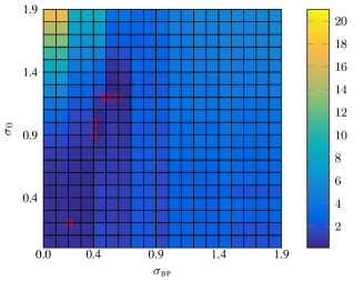
Figure 7: Error as function of pre-smoothing the image with a Gaussian kernel of standard deviation of $\sigma_{0}$ as as well smoothing the Bit-Planes with $\sigma_{1}$. The lowest error is associated with smaller kernels.

V-C Runtime

There are two steps to the algorithm. First, is pre-computing the Jacobian of the cost function as well as the Bit-Planes descriptor for the reference image. This is required only when a new keyframe is created. We call this step Jacobians. The second step, which is repeated at every iteration consists of: (i) image warping using the current estimate of pose, (ii) computing the Bit-Planes error, (iii) computing the residuals and estimating their standard deviations, and (iv) building the weighted linear system and solving it. We call this image Linearization. The running time for each step is summarized in Table I as a function of image resolution and the selected image points. A typical number of iterations for a run using stereo computed with block matching is shown in Figs. 8 and 9. The bottleneck in the Linearization step is computing the median absolute deviation of the residuals, which could be mitigated by approximating the median with histograms [34]. Timing for each of the major steps is shown in Tables I and II.

TABLE I: Execution time of each major step in the algorithm reported in milliseconds (ms) and using four pyramid levels. The construction of the image pyramid is a common step for both raw intensity and Bit-Planes. Descriptor computation step for raw intensity amounts to converting the image to floating point. Jacobian pre-computation is required only when creating a new keyframe. The most commonly performed operation is descriptor warping, which is not significantly more expensive than warping a single channel of raw intensity. Note, both descriptors (raw intensity and Bit-Planes) use the same generic code base. It is possible to obtain additional speedups by optimizing the code for Bit-Planes specifically. For larger images see Table II.

	Raw Intensity	Bit-Planes
Pyramid construction	$0.31$
Descriptor computation	$0.18$	$4.33$
Jacobian pre-computation	$3.34$	$10.47$
Descriptor warping	$0.35$	$1.65$

TABLE II: Execution time of each major step of the algorithm using the KITTI dataset with image size $1024\times 376$. Please refer to Table I for details.

	Raw Intensity	Bit-Planes
Pyramid construction	$0.44$
Descriptor computation	$0.28$	$5.55$
Jacobian pre-computation	$5.00$	$13.92$
Descriptor warping	$0.30$	$1.74$

Figure 8: Number of iterations and runtime on the first $500$ frames of the New Tsukuba dataset using raw intensity only. On average, the algorithm runs at more than $100$ Hz.

Figure 9: Number of iterations and run time using on the first $500$ frames of the New Tsukuba dataset using the Bit-Planes descriptors. On average, the algorithm runs at $15$ Hz.

V-D Experiments with synthetic data

We use the “New Tsukuba” dataset [46, 39] to compare the performance of our algorithm against two representative algorithms from the state-of-the-art. The first, is FOVIS [28], which we use as a representative of feature-based methods. The second, is DVO [32] as representative of direct methods using the brightness constancy assumption. The most challenging illumination condition provided by the Tsukuba dataset is when the scene is lit by “lamps” as shown in Fig. 12, which we use in our evaluation.

Our goal is this experiment is to assess the utility of our proposed descriptor in handling the arbitrary change in illumination visible in all frames of the dataset. Hence, we initialize all algorithms with the ground truth disparity/depth map. In this manner, any pose estimation errors are caused by failures to extract and match features, or failure in minimizing the photometric error. As shown in Fig. 10 and Fig. 11 the robustness of our approach far exceeds the conventional state-of-the-art. Also, as expected, feature-based methods in this case (FOVIS) slightly outperforms direct methods (DVO) due to the challenging illumination of the scene.

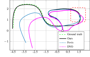
Figure 10: Evaluation on the synthetic Tsukuba sequence [46] using the illumination provided by “lamps” in comparison to other VO algorithms. The figure shows a bird’s eye view of the estimated trajectory of the camera form each algorithm in comparison to the ground truth. The highlighted area is shown with more details in Fig. 11. Example images are in Fig. 12.

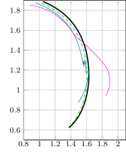
Figure 11: Estimated camera path details for each of the algorithms shown in Fig. 10.

.

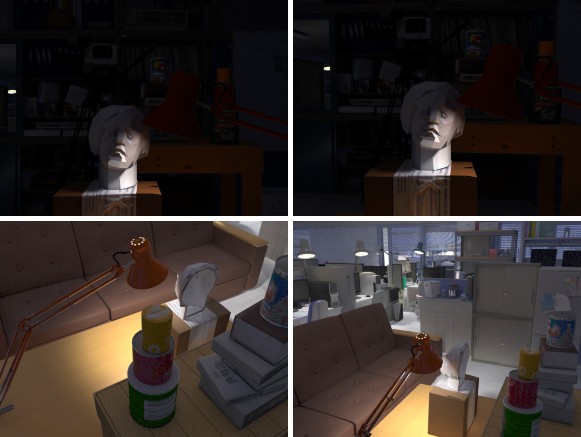
Figure 12: Example images from the “lamps” sequence.

V-E Evaluation on the KITTI benchmark

The KITTI benchmark [21] presents a challenging dataset for our algorithm, and all direct methods in general, as the motion between consecutive frames is large. The effect of large motions can be observed in Fig. 13, where the performance of our algorithm noticeably degrades at higher vehicle speeds. This limitation could be mitigated by using a higher camera frame rate, or providing a suitable initialization.

Figure 13: Performance on the training data of the KITTI benchmark in comparison to VISO2 [20]. The large baseline between consecutive frames presents a challenge to direct methods as can been seen by observing the error as a function of speed. Nonetheless, rotation accuracy of our method remains high.

V-F Real data from underground mines

We demonstrate the robustness of our algorithm using data collected in underground mines. Our robot is equipped with a stereo camera with $7$cm baseline that outputs grayscale images of size $1024\times 544$ and computes an estimate of disparity using a hardware implementation of SGM [25]. An example VO result along with a sample of the data is shown in Fig. 14.

Due to lack of lighting in underground mines, the robot carries its own source of LED light. However, the LEDs are insufficient to uniformly illuminate the scene due to power constraints in the system. We have attempted to use other open source VSLAM/VO packages [28, 42, 20], but they all fail too often due to the severely degraded illumination conditions.

In Fig. 15, we show another result from a different underground environment where the stereo 3D points are colorized by height. The large empty areas in the generated map is due to lack of disparity estimates in large portions of the input images. Due to lack of ground-truth we are unable to assess the accuracy of the system. But, visual inspection of the created 3D maps indicate minimal drift, which is expected when operating in an open loop fashion.

(a) Long section of $\approx 400$ meters of robust VO in a poorly lit underground environments.

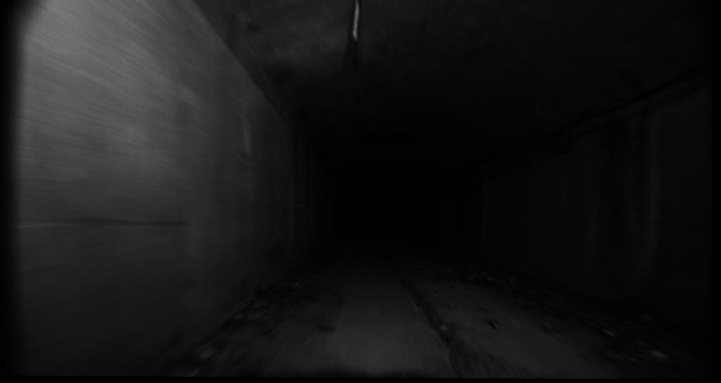
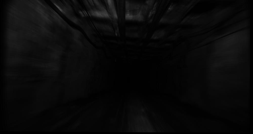
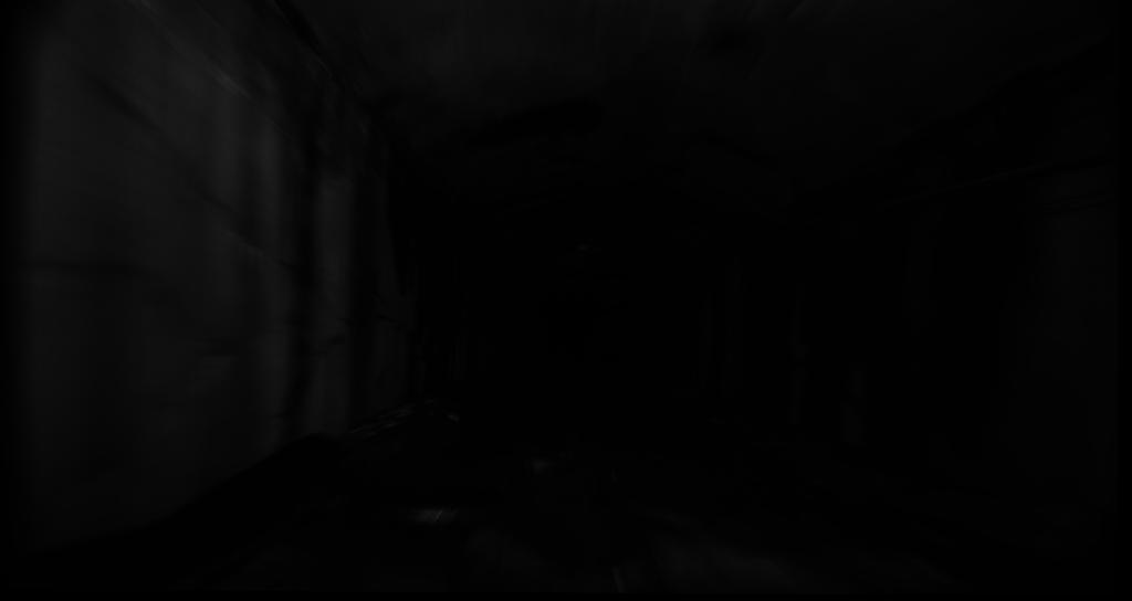
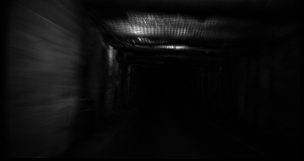
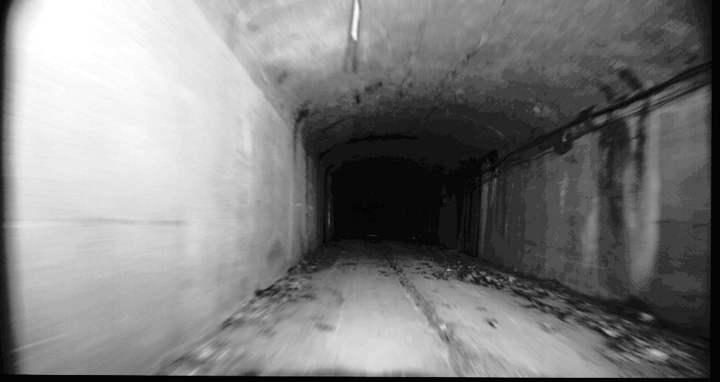
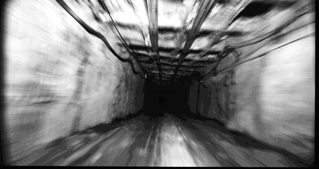
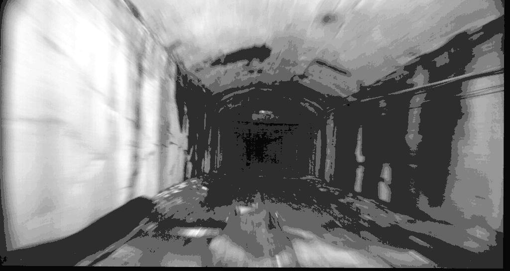
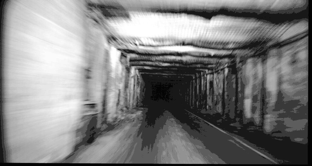
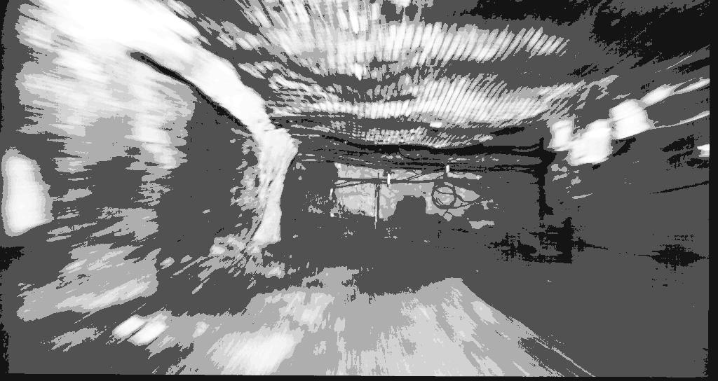
Figure 14: Example result and representative images from the first mine sequence (top row) and a histogram equalized version for visualization (bottom row).

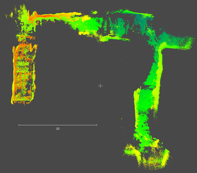
Figure 15: VO map colorized by height showing the robot transitioning between different levels in the second mine dataset.

V-G Reconstruction density

Density of the reconstructed point cloud is demonstrated in Fig. 16 and Fig. 17. Denser output is possible by eliminating the pixel selection step at the expense of increased computational time.

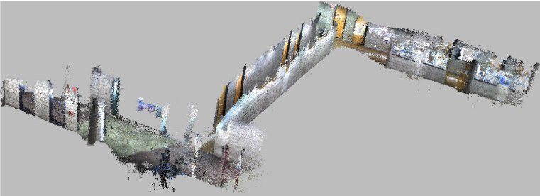
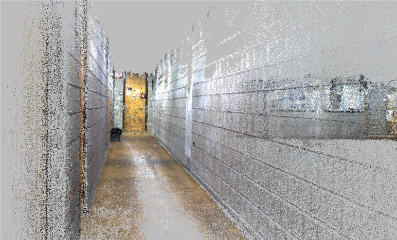
Figure 16: Reconstruction density using an indoor dataset collected by us [2].

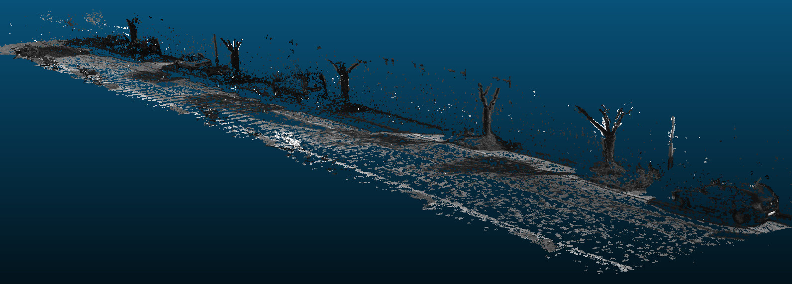
Figure 17: Reconstruction density on a section of the KITTI dataset.

V-H Failure cases

Most failure cases are due to a complete image washout. An example is shown in Fig. 18. Theses cases occur when the robot is navigating a tight turn such that all of the LED output is constrained very closely to the camera. Addressing such cases, form vision-only data, is a good avenue of future work.

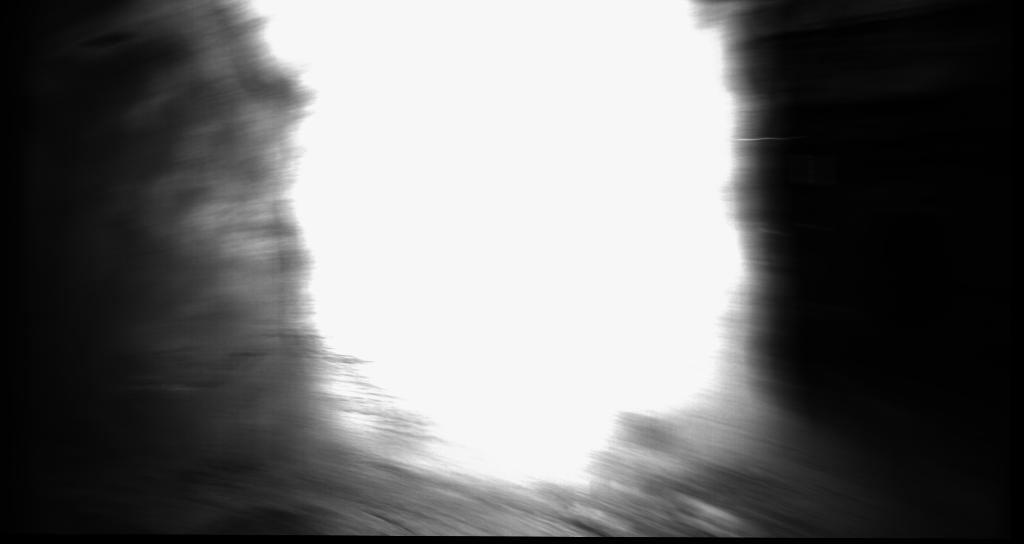
Figure 18: An example of a failure case where most of the image details are washed out causing complete loss of stereo.

VI Conclusion

In this work, we presented a VO system capable of operating in challenging environments where the illumination of the scene is poor and non-uniform. The approach is based on direct alignment of feature descriptors. In particular, we designed an efficient to compute binary descriptor that is invariant to monotonic changes in intensity. By using this descriptor constancy, we allow vision-only pose estimation to operate robustly in environments that lack keypoints and lack the photometric consistency required by direct methods.

Our descriptor, Bit-Planes, is designed for efficiency. However, other descriptors could be used instead (such ORB and/or SIFT) if computational demands are not an issues. A comparison of performance between difference descriptors in a direct framework is an interesting direction of future work as their amenability to linearization may differ.

The approach is simple to implement, and can be readily integrated into existing direct VSLAM algorithms with a small additional computational overhead.

References

- Alismail and Browning [2014] Hatem Alismail and Brett Browning. Direct Disparity Space: An Algorithm for Robust and Real-time Visual Odometry. Technical Report CMU-RI-TR-14-20, Robots Institute, Oct 2014.
- Alismail et al. [2010] Hatem Alismail, Brett Browning, and M Bernardine Dias. Evaluating Pose Estimation Methods for Stereo Visual Odometry on Robots. In the 11th Int’l Conf. on Intelligent Autonomous Systems (IAS-11), 2010.
- Alismail et al. [2016] Hatem Alismail, Brett Browning, and Simon Lucey. Bit-Planes: Dense Subpixel Alignment of Binary Descriptors. CoRR, abs/1602.00307, 2016.
- Antonakos et al. [2015] E. Antonakos, J. Alabort-i Medina, G. Tzimiropoulos, and S.P. Zafeiriou. Feature-Based Lucas-Kanade and Active Appearance Models. Image Processing, IEEE Transactions on, 24(9):2617–2632, Sept 2015.
- Badino et al. [2013] Hernán Badino, Akihiro Yamamoto, and Takeo Kanade. Visual odometry by multi-frame feature integration. In Computer Vision Workshops (ICCVW), 2013 IEEE International Conference on, pages 222–229, 2013.
- Baker and Matthews [2004] Simon Baker and Iain Matthews. Lucas-kanade 20 years on: A unifying framework. International Journal of Computer Vision, 56(3):221–255, 2004.
- Beaton and Tukey [1974] Albert E. Beaton and John W. Tukey. The Fitting of Power Series, Meaning Polynomials, Illustrated on Band-Spectroscopic Data. Technometrics, 16(2):pp. 147–185, 1974. ISSN 00401706.
- Bilaniuk et al. [2014] O. Bilaniuk, E. Fazl-Ersi, R. Laganiere, C. Xu, D. Laroche, and C. Moulder. Fast LBP Face Detection on Low-Power SIMD Architectures. In Computer Vision and Pattern Recognition Workshops (CVPRW), 2014 IEEE Conference on, pages 630–636, June 2014.
- Bordallo López et al. [2014] Miguel Bordallo López, Alejandro Nieto, Jani Boutellier, Jari Hannuksela, and Olli Silvén. Evaluation of real-time LBP computing in multiple architectures. Journal of Real-Time Image Processing, pages 1–22, 2014. ISSN 1861-8200. doi: 10.1007/s11554-014-0410-5.
- Bristow and Lucey [2014] Hilton Bristow and Simon Lucey. In Defense of Gradient-Based Alignment on Densely Sampled Sparse Features. In Dense correspondences in computer vision. Springer, 2014.
- Brox et al. [2004] Thomas Brox, Andres Bruhn, Nils Papenberg, and Joachim Weickert. High Accuracy Optical Flow Estimation Based on a Theory for Warping. In ECCV, volume 3024 of Lecture Notes in Computer Science, pages 25–36. Springer Berlin Heidelberg, 2004.
- Comport et al. [2010] Andrew I Comport, Ezio Malis, and Patrick Rives. Real-time quadrifocal visual odometry. The International Journal of Robotics Research, 29(2-3):245–266, 2010.
- Crivellaro and Lepetit [2014] Alberto Crivellaro and Vincent Lepetit. Robust 3D Tracking with Descriptor Fields. In Conference on Computer Vision and Pattern Recognition (CVPR), 2014.
- Dalal and Triggs [2005] N. Dalal and B. Triggs. Histograms of oriented gradients for human detection. In Computer Vision and Pattern Recognition (CVPR). IEEE Computer Society Conference on, volume 1, pages 886–893 vol. 1, June 2005.
- Dame and Marchand [2010] A. Dame and E. Marchand. Accurate real-time tracking using mutual information. In Mixed and Augmented Reality (ISMAR), 2010 9th IEEE International Symposium on, pages 47–56, Oct 2010.
- Dowson and Bowden [2008] N. Dowson and R. Bowden. Mutual Information for Lucas-Kanade Tracking (MILK): An Inverse Compositional Formulation. PAMI, 30(1):180–185, Jan 2008.
- Engel et al. [2015] J. Engel, J. Stueckler, and D. Cremers. Large-Scale Direct SLAM with Stereo Cameras. In International Conference on Intelligent Robots and Systems (IROS), 2015.
- Engel et al. [2014] Jakob Engel, Thomas Schöps, and Daniel Cremers. LSD-SLAM: Large-Scale Direct Monocular SLAM. In ECCV, 2014.
- Forster et al. [2014] Christian Forster, Matia Pizzoli, and Davide Scaramuzza. SVO: Fast Semi-Direct Monocular Visual Odometry. In Proc. IEEE Intl. Conf. on Robotics and Automation (ICRA), 2014.
- Geiger et al. [2011] Andreas Geiger, Julius Ziegler, and Christoph Stiller. StereoScan: Dense 3d Reconstruction in Real-time. In Intelligent Vehicles Symposium (IV), 2011.
- Geiger et al. [2012] Andreas Geiger, Philip Lenz, and Raquel Urtasun. Are we ready for Autonomous Driving? The KITTI Vision Benchmark Suite. In Conference on Computer Vision and Pattern Recognition (CVPR), 2012.
- Gennert and Negahdaripour [1987] Michael A Gennert and Shahriar Negahdaripour. Relaxing the brightness constancy assumption in computing optical flow, 1987.
- Henry et al. [2012] Peter Henry, Michael Krainin, Evan Herbst, Xiaofeng Ren, and Dieter Fox. RGB-D mapping: Using Kinect-style depth cameras for dense 3D modeling of indoor environments. IJRR, 31(5):647–663, 2012.
- Herout et al. [2010] Adam Herout, Roman Juránek, and Pavel Zemčík. Implementing the Local Binary Patterns with SIMD instructions of cpu. In Proceedings of WSCG 2010, pages 39–42. University of West Bohemia in Pilsen, 2010. ISBN 978-80-86943-86-2.
- Hirschmuller [2005] H. Hirschmuller. Accurate and efficient stereo processing by semi-global matching and mutual information. In Computer Vision and Pattern Recognition, 2005.
- Horn and Schunck [1981] Berthold KP Horn and Brian G Schunck. Determining optical flow. Artificial intelligence, 17(1):185–203, 1981.
- Howard [2008] A Howard. Real-time stereo visual odometry for autonomous ground vehicles. In Int’l Conf. on Intelligent Robots and Systems, 2008.
- Huang et al. [2011] Albert S Huang, Abraham Bachrach, Peter Henry, Michael Krainin, Daniel Maturana, Dieter Fox, and Nicholas Roy. Visual odometry and mapping for autonomous flight using an RGB-D camera. In International Symposium on Robotics Research (ISRR), pages 1–16, 2011.
- Irani and Anandan [1998] M. Irani and P. Anandan. Robust multi-sensor image alignment. In Computer Vision, 1998. Sixth International Conference on, pages 959–966, Jan 1998.
- Irani and Anandan [2000] M. Irani and P. Anandan. About Direct Methods. In Vision Algorithms: Theory and Practice, pages 267–277, 2000.
- Kaess et al. [2009] M. Kaess, Kai Ni, and F. Dellaert. Flow separation for fast and robust stereo odometry. In IEEE Conf. on Robotics and Automation, pages 3539–3544, May 2009.
- Kerl et al. [2013a] Christian Kerl, J. Sturm, and D. Cremers. Robust Odometry Estimation for RGB-D Cameras. In Int’l Conf. on Robotics and Automation (ICRA), May 2013a.
- Kerl et al. [2013b] Christian Kerl, Jurgen Sturm, and Daniel Cremers. Dense visual slam for RGB-D cameras. In Int’l Conf. on Intelligent Robots and Systems, 2013b.
- Klose et al. [2013] Sebastian Klose, Philipp Heise, and Alois Knoll. Efficient compositional approaches for real-time robust direct visual odometry from RGB-D data. In IEEE/RSJ Int’l Conf. on Intelligent Robots and Systems, 2013.
- Lowe [2004] David G. Lowe. Distinctive Image Features from Scale-Invariant Keypoints. International Journal of Computer Vision, 60(2):91–110, 2004.
- Lu and Song [2015] Yan Lu and Dezhen Song. Robustness to lighting variations: An RGB-D indoor visual odometry using line segments. In Intelligent Robots and Systems (IROS), IEEE/RSJ International Conference on, 2015.
- Lucas and Kanade [1981] Bruce D. Lucas and Takeo Kanade. An Iterative Image Registration Technique with an Application to Stereo Vision (DARPA). In Proc. of the 1981 DARPA Image Understanding Workshop, pages 121–130, April 1981.
- Maimone et al. [2007] Mark Maimone, Yang Cheng, and Larry Matthies. Two years of visual odometry on the Mars Exploration Rovers. Journal of Field Robotics, Special Issue on Space Robotics, 24, 2007.
- Martull et al. [2012] Sarah Martull, Martin Peris, and Kazuhiro Fukui. Realistic CG stereo image dataset with ground truth disparity maps. In ICPR workshop TrakMark2012, volume 111, pages 117–118, 2012.
- Meilland et al. [2012] M. Meilland, P Rives, and A. I. Comport. Dense RGB-D mapping for real-time localisation and navigation. In IV12 Workshop on Navigation Positionnig and Mapping, Alcalá de Henares, Spain., June 3 2012.
- Milford et al. [2014] Michael Milford, Eleonora Vig, Walter Scheirer, and David Cox. Vision-based Simultaneous Localization and Mapping in Changing Outdoor Environments. Journal of Field Robotics, 31(5):780–802, 2014.
- Mur-Artal et al. [2015] Raul Mur-Artal, J. M. M. Montiel, and Juan D. Tardós. ORB-SLAM: a Versatile and Accurate Monocular SLAM System. CoRR, abs/1502.00956, 2015.
- Newcombe et al. [2011] R.A. Newcombe, S.J. Lovegrove, and A.J. Davison. DTAM: Dense tracking and mapping in real-time. In Computer Vision (ICCV), 2011 IEEE International Conference on, pages 2320–2327, Nov 2011.
- Nister et al. [2004] D. Nister, O. Naroditsky, and J. Bergen. Visual odometry. In Computer Vision and Pattern Recognition (CVPR), June 2004.
- Ojala et al. [1996] Timo Ojala, Matti Pietikäinen, and David Harwood. A comparative study of texture measures with classification based on featured distributions. Pattern Recognition, 29:51–59, 1996.
- Peris et al. [2012] M. Peris, A Maki, S. Martull, Y. Ohkawa, and K. Fukui. Towards a simulation driven stereo vision system. In Pattern Recognition (ICPR), 2012 21st International Conference on, pages 1038–1042, Nov 2012.
- Rublee et al. [2011] E. Rublee, V. Rabaud, K. Konolige, and G. Bradski. ORB: An efficient alternative to SIFT or SURF. In Computer Vision (ICCV), 2011 IEEE International Conference on, pages 2564–2571, Nov 2011.
- Sevilla-Lara et al. [2014] Laura Sevilla-Lara, Deqing Sun, Erik G. Learned-Miller, and Michael J. Black. Computer Vision – ECCV 2014: 13th European Conference, Zurich, Switzerland, September 6-12, 2014, Proceedings, Part I, chapter Optical Flow Estimation with Channel Constancy, pages 423–438. Springer International Publishing, Cham, 2014. ISBN 978-3-319-10590-1. doi: 10.1007/978-3-319-10590-1˙28.
- Silveira and Malis [2007] G. Silveira and E. Malis. Real-time Visual Tracking under Arbitrary Illumination Changes. In Computer Vision and Pattern Recognition, 2007. CVPR ’07. IEEE Conference on, pages 1–6, June 2007.
- Song and Klette [2013] Zijiang Song and Reinhard Klette. Robustness of Point Feature Detection. 2013.
- Steinbrucker et al. [2011] F Steinbrucker, Jürgen Sturm, and Daniel Cremers. Real-time visual odometry from dense RGB-D images. In ICCV Workshops, IEEE Int’l Conf. on Computer Vision, 2011.
- Torr and Zisserman [2000] P.H.S. Torr and A. Zisserman. Feature Based Methods for Structure and Motion Estimation. In Vision Algorithms: Theory and Practice, pages 278–294. Springer Berlin Heidelberg, 2000.
- Vogel et al. [2013] Christoph Vogel, Stefan Roth, and Konrad Schindler. An Evaluation of Data Costs for Optical Flow. In Joachim Weickert, Matthias Hein, and Bernt Schiele, editors, Pattern Recognition, Lecture Notes in Computer Science. Springer Berlin Heidelberg, 2013. ISBN 978-3-642-40601-0. doi: 10.1007/978-3-642-40602-7˙37.
- Whelan et al. [2013] T. Whelan, H. Johannsson, M. Kaess, J.J. Leonard, and J. McDonald. Robust real-time visual odometry for dense RGB-D mapping. In IEEE Proc. of Intl’ Conf. on Robotics and Automation (ICRA), May 2013.
- Zabih and Woodfill [1994] Ramin Zabih and John Woodfill. Non-parametric local transforms for computing visual correspondence. In Computer Vision - ECCV’94, pages 151–158. Springer, 1994.
- Zhang [1997] Zhengyou Zhang. Parameter estimation techniques: A tutorial with application to conic fitting. Image and vision Computing, 15(1), 1997.