Progressive Temporal Window Widening

Abstract

This paper introduces a scheme for data stream processing which is robust to batch duration. Streaming frameworks process streams in batches retrieved at fixed time intervals. In a common setting a pattern recognition algorithm is applied independently to each batch. Choosing the right time interval is tough — a pattern may not fit in an interval which is too short, but detection will be delayed and memory may be exhausted if the interval is too long. We propose here Progressive Window Widening, an algorithm for increasing the interval gradually so that patterns are caught at any pace without unnecessary delays or memory overflow.

This algorithm is relevant to computer security, system monitoring, user behavior tracking, and other applications where patterns of unknown or varying duration must be recognized online in data streams. Modern data stream processing frameworks are ubiquitously used to process high volumes of data, and adaptive memory and CPU allocation, facilitated by Progressive Window Widening, is crucial for their performance.

1 Introduction

We consider here the problem of windowed data stream processing [7]. A data stream is a real-time, continuous, ordered sequence of items. In the windowed setting, the arriving data are divided into windows, either by time interval or by data size, and a pattern recognition algorithm, based on a data mining or machine learning approach, is applied to each window to discover exact or approximate patterns appearing in the window [6]. Here, we view a pattern recognition algorithm as a black box function on stream fragments. For example, a pattern can be an episode — a partially ordered sparse subsequence [10], the language of the text, or the most likely goal of the sequence of actions in the fragment.

Windowed data stream processing is frequently used in computer security [12, 11, 14], user behavior tracking [2], sensor data analysis for system monitoring [3], and other applications. The right choice of window size is crucial for efficient data processing and timely response. Data are divided either into physical windows, by time interval, or into logical, or count-based, windows, by data size or number of records in a single window [7, 6].

The choice of either physical or logical windows depends both on properties of the data stream and on the objective of the data processing algorithm. Logical windows are more naturally handled by machine learning algorithms with inputs of fixed size [6], while physical windows allow both more efficient processing and faster online response [9, 17, 16]. This paper explores selecting a window size for physical, interval-based windows. The dilemma behind selecting a window size which inspired this research is

• whether to choose a smaller window and sacrifice context, such that no single window contains a complete pattern,

• or to increase the window size at the cost of increased consumption of computational resources and delayed response.

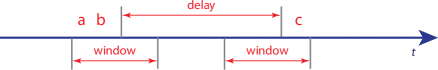
Figure 1: Adversary escaping detection. Pattern $a,b,c$ cannot be caught because the delay between $b$ and $c$ is longer than the window duration.

This dilemma is relevant to many applications of data stream processing, but in particular to security applications [12, 11, 14], where an adversary aware of the maximum window time interval can escape the detection algorithm by introducing delays between data stream entries (such as transactions or web site accesses) which exceed the interval and prevent detection (Figure 1). Even if the maximum duration of a pattern is known in advance, setting the window size to exceed the maximum duration means that recognition of any shorter pattern will be delayed.

To address this dilemma, we introduce an algorithm which we call Progressive Window Widening (PWW). PWW processes the data stream through an array of sliding windows of increasing physical size, such that shorter patterns are recognized sooner, however windows covering longer patterns are also applied to the stream. Despite employing several window sizes in parallel, PWW still remains efficient in CPU and memory consumption. The paper proceeds as follows: first, necessary preliminaries are introduced in Section 2. Then, the algorithm is described and analysed (Sections 3 and 4), as well as evaluated empirically (Section 5). Finally, related work is reviewed, and contribution and future research are discussed (Sections 6 and 7).

2 Preliminaries

2.1 Batched Stream Processing

In batched stream processing, which we adopt in this paper as a lower level for PWW, stream data arrives in batches — sequences of fixed duration. Several batches can be combined into a window of size equal to the total size of the batches composing the window. Along with batch size (or duration, used interchangeably here), a batch is characterized by its length, the number of atomic elements, or records, it contains. For example, a one-minute batch of web site log stream may contain 1000 entries — we shall say that the size, or duration of the batch is 1 minute, and the length of the batch is 1000 entries.

Further on, we extend the note of batched stream processing by stating that a data stream with batch duration $t$ may be transformed into a data stream with batch duration $kt$ by concatenating each $k$ consecutive batches together. Denoting a batch of the original stream with batch duration $t$ by $B_{i,l}$ and a batch of the combined stream with batch duration $kt$ by $B_{i+1,j}$ for some $i$, $j$, and $l$, one may write ($\circ$ stands for batch concatenation):

$$B_{i+1,j}=B_{i,kj-k+1}\circ B_{i,kj-k+2}\circ\dots\circ B_{i,kj}\quad\forall j\in\mathbb{N}^{+}$$ (1)

2.2 Sliding Windows

Depending on the overlay between windows, one discerns between tumbling (there are gaps between windows), jumping (the windows are adjacent), and sliding (overlapping) windows [7]. PWW is based on sliding windows; the next window starts earlier than the current window terminates.

Sliding windows have several uses. We are interested in one particular case: sliding windows with a half-size overlap; the feature we are interested in is described by Lemma 1:

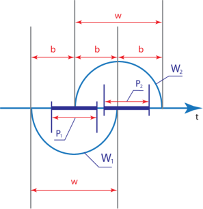
Figure 2: Pattern recognition in sliding windows. If we want to recognize patterns of duration at most $t$, it is sufficient to use sliding windows of size $2t$ with half-size overlap.

Lemma 1

A sequence of sliding windows of size $2b$ with overlap $b$ covers any interval of size at most $b$.

Proof

Indeed, divide the stream into batches of size $b$ (Figure 2). Any interval of size at most $b$ is either entirely within a single batch, or spans two consequent batches. But every single batch, and every pair of consequent batches is covered by a single window. This completes the proof.

A corollary of Lemma 1 is that if we want to recognize patterns of duration at most $t$, it is sufficient to use sliding windows of size $2t$ with half-size overlap.

3 Progressive Window Widening

We introduce here Progressive Window Widening, an algorithm for progressive widening of temporal windows. To define the algorithm efficiently, we rely on two auxiliary notions:

• $L_{max}$ — the maximum length of a data sequence which may contain a pattern. For example, if a game player must complete each game round in 20 moves, than any pattern pertaining to a single round must be contained within 20 moves. Alternatively, $L_{max}$ can be chosen such that the probability of a random occurence of the pattern in a data sequence of length $L_{max}$ is sufficiently low [8].

• $T_{max}$ — the upper bound on pattern duration. For example, if a computer is rebooted every week, then the longest duration of a running process is one week, or $604\,800$ (less than $2^{20}$) seconds. $T_{max}$ is not strictly required for the definition of the algorithm but helps in the algorithm’s implementation.

The algorithm processes the data stream in parallel, through multiple asynchronous sliding windows of different sizes.

3.1 Algorithm Outline

1:  procedure PWW($S$ – stream, $t$ – batch duration)

2:  Sleep($t$)

3:  Create stream $S^{\prime}$ from $S$ with batch duration $2t$ (see Algorithm 2)

4:  Call PWW($S^{\prime}$, $2t$) asynchronously

5:  for each sliding window $W$ in $S$ do

6:     if patterns present in $W$ then

7:        Output detected patterns

8:     end if

9:  end for

Algorithm 1 Progressive Window Widening

PWW (Algorithm 1) performs the following operations:

1. Recursively combines pairs of adjacent batches, doubling batch duration of each stream and creating a stream with batches of double duration (line 3).

2. Runs a detection algorithm in a sliding window on each stream (line 6).

3. While combining batches, discards subintervals of combined batches which cannot intersect a yet unseen pattern (see Section 3.2 for detailed explanation).

As the algorithm runs, multiple batched streams are created, and sliding windows move through each of the streams (Figure 3). The algorithm relies on asynchronous recursive calls to PWW (line 4). Asynchronous calls are possible because the processing of each stream is independent. Such asynchronous execution is particularly suitable for modern multi-core multi-node cluster architectures: different invocations of PWW may be executed on different cores or different nodes in the cluster.

Note that extra streams are created (lines 2–4) and processed (line 5) with exponentially increasing delays, since a window can be processed only upon termination of the window’s interval.

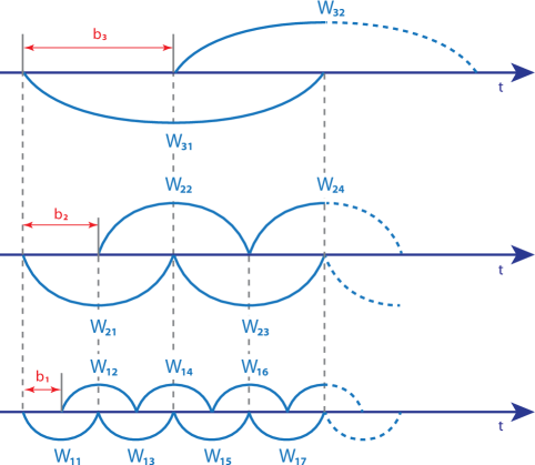
Figure 3: Window widening. Multiple sliding windows of increasing durations are processed in parallel, with delay.

3.2 Combining batches

An integral part of PWW is the optional discarding of a subinterval while combining two subsequent batches. For every stream of batches of duration $t$, the algorithm waits $2t$ time units for 2 batches to arrive. Then, a stream of base duration $2t$ is formed by combining the batches (Algorithm 2).

1:  procedure Combine($B_{i-1,2j-1}$, $B_{i-1,2j}$ – consequent batches)

2:  $B_{i,j}$ $\leftarrow$ Concatenate($B_{i-1,2j-1}$, $B_{i-1,2j}$)

3:  if Length($B_{i,j}$) $>2L_{max}$ then

4:     Remove($B_{i,j}$, from=$L_{max}$, till=Length($B_{i,j}$)$-L_{max}$)

5:  end if

6:  return  $B_{i,j}$

Algorithm 2 Combining Batches

PWW combines batches by concatenation (line 2). If the length of the combined batch is greater than $2L_{max}$, the middle part of the combined batch is discarded (Figure 4), leaving subsequences of length $L_{max}$ at both ends of the batch (lines 3–5).

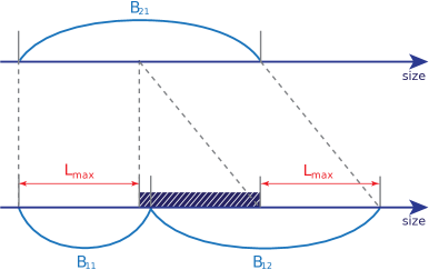
Figure 4: Removing useless data from batches. Since no pattern can span a fragment of more than $L_{max}$ items, the middle part of the combined batch can be discarded. Only subsequences of length $L_{max}$ at the ends of the batch must be kept.

Consequently, no batch in any stream is longer than $2L_{max}$. The subintervals may be discarded because a combined batch at the next level coincides with a sliding window at the current level, so new patterns may be discovered only between batches, rather than within a single batch.

4 Algorithm Analysis

In this section we show that the algorithm eventually has a chance to detect a pattern of any duration and, at the same time, runs in bounded resources.

4.1 Correctness

Since window duration is unbounded, to prove the correctness we just need to show that discarded intervals do not intersect any pattern which did not fall entirely within a single window.

Theorem 1

Any pattern of length at most $L_{max}$ is contained in a window.

Proof

Indeed, as we noted earlier, a combined batch at the next level coincides with a single sliding window at the current level. Any pattern which is contained in a sliding window could be seen by the pattern recognition algorithm, and the interval containing the pattern can be discarded. Hence, a yet unseen pattern intersecting a window must cross one of the ends of the window (and of the combined batch at the next level).

Since every combined batch with a discarded subinterval has $L_{max}$ contiguous elements adjacent to each of the ends, the discarded interval does not intersect with a pattern of length at most $L_{max}$. This completes the proof.

4.2 Complexity

We launch an unbounded number of parallel processes, and want to show that PWW runs in computationally bounded resources. The work that the algorithm performs is assumed to take place inside a pattern recognition algorithm run on each sliding window. Let us denote the resources (a combination of memory and amount of work) required to run a certain pattern recognition algorithm on window of length $l$ by $\mathcal{R}(l)$. Then, the following theorem holds:

Theorem 2

Denote by $t$ the batch duration of the initial, uncombined stream. Assume that the maximum length of a batch of the initial stream does not exceed $2L_{max}$. Then the average resources $\rho$ per unit time required to run PWW are bounded by a constant:

$$\rho\leq\frac{2\mathcal{R}(4L_{max})}{t}\,.$$ (2)

Proof

Due to Algorithm 2, the length of a sliding window is at most $4L_{max}$, hence running the pattern recognition algorithm on a window requires at most $\mathcal{R}(4L_{max})$ resources.

Windows in streams are processed sequentially, and a window in the $i$th stream arrives after delay $2^{i-1}t$. Therefore,

$$\rho\leq\sum_{i=1}^{\infty}\frac{\mathcal{R}(4L_{max})}{2^{i}t}=\frac{\mathcal{R}(4L_{max})}{t}\sum_{i=1}^{\infty}\frac{1}{2^{i-1}}=\frac{2\mathcal{R}(4L_{max})}{t}\,.$$ (3)

This completes the proof.

Note that the assumption in Theorem 2 is satisfied by choosing the initial batch duration $t$ to be small enough. On the other hand, it may be the case that the length of a batch at any intermediate level reaches $2L_{max}$ (and then the data in the batch is partially disregarged, as detailed in Section 3.2.

In practice, the number of parallel streams may be bounded. However, even if unbounded, average resources required to run the algorithm are bounded.

5 Case Study: Detecting Remote Shells in a System Call Stream

In this case study, we monitor an online stream of system calls from a network-connected server, and want to detect possible invocations of remote shells as soon as possible. System call traces are represented according to the following format:

system-call [argument ...] [=> return-value]

A line consists of the system call name, followed by optional arguments, followed by optional return value preceded by =>. Each argument is a name-value pair, with the name separated from the value by =. System call sequences corresponding to remote shell invocations can be interspersed with unrelated activities.

For simplicity, we limit detection to a single episode which may correspond to accepting a network connection and then launching a shell communicating with the remote user through the connection:

1 accept fd=x => y
2 dup fd=y => 0 | dup fd=y => 1 | dup fd=y => 2
3 execve exe=z

In the above pseudocode, system call name is followed by name=value argument pairs and then by return value preceded by =>. In a matching system call sequence y must have the same value in lines 1 and 2, three system calls in line 2 may be executed in any order, and x, z may take any value. For example, sequence

accept fd=5 => 6
dup fd=6 => 2
dup fd=6 => 1
dup fd=6 => 0
execve exe=sh

matches the episode.

For the empirical evaluation we use a sequential version of PWW which facilitates easy estimation of the amount of work. We set $L_{max}=100$ because malicious code is often transmitted in a single packet with only a few dozens of instructions. For simplicity, we assume that one system call arrives per time unit. We use a stream of $10\,000$ system calls recorded on a Linux machine, into which we inject episode instances with varying delays between instructions. As a baseline, we use a fixed duration window of $200$ time units. We find that:

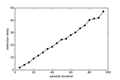
Figure 5: Detection delay. The delay grows linearly with shell code duration, with factor 0.5, as expected. In other words, by linearly increasing the amount of work we are able to detect patterns with delay which is only half of the pattern duration.

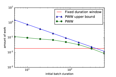
Figure 6: Amount of work. The amount of work of PWW (green) approaches but stays below the theoretical bound (blue). The amount of work of PWW is lower than of fixed duration window (red) for sufficiently large initial batch duration.

• The detection delay (Figure 5) is proportional to the episode duration with factor 0.5.

• The amount of work (Figure 6) approaches but stays below bound (2) as the initial batch duration grows. For sufficiently large initial batch duration, the amount of work of PWW is lower than of fixed window duration.

The results are in accordance with the algorithm analysis. If a fixed duration window were used, either the average detection delay would be larger, or some episodes were left undetected. PWW ensures timely detection of episodes of any duration at the cost of only a constant factor increase in the amount of work.

The source code, data, and results for the case study are available at https://bitbucket.org/dtolpin/pww-paper-case-studies. The evaluation notebook can be viewed in the browser at http://tinyurl.com/jgknulz.

6 Related Work

While Progressive Window Widening can be implemented from scratch on low-level data streams, the algorithm was inspired and relies in implementation on batched stream processing. Batch stream processing was introduced in Comet [9]. Apache Spark offers Spark Streaming [17, 16], a powerful implementation of programming model discretized streams. Discretized streams, which enable efficient batch processing in parallel architectures, is the enabling lower level for PWW.

PWW uses varying window sizes to accommodate for differences in data. Another approach in batched stream processing is to use adaptive window size. Adaptive window algorithms is a field of active research [18, 4, 5, 13]. However, this research represents a different approach, in which the window size is changed sequentially and adaptively, for future windows based on earlier seen data. In PWW, several windows of fixed sizes are applied in parallel, in a parameter-free manner suitable for simple and robust implementation. Windows of doubling size were proposed for processing data streams in earlier work [1], however the approach employed in PWW is significantly different in that temporal windows of unbounded doubling durations are applied in parallel, while still ensuring efficient use of resources.

7 Contribution and Future Research

This paper introduced the Progressive Window Widening algorithm for data stream processing using temporal sliding windows. The algorithm

• solves the dilemma of smaller window size at a cost of inability to recognize longer patterns versus larger windows but slower response;

• works in parallel, in a manner suitable for modern multi-core multi-node cluster architectures;

• uses computational resources efficiently, imposing only a constant factor overhead compared to an algorithm based on a single window size.

The basic algorithm described in the paper brings a solution to the stated problem. At the same time, the algorithm design poses a number of questions and opens several research directions.

• Many adaptive window algorithms are, unlike PWW, essentially sequential. Modern data frameworks provide an opportunity to exploit the parallelism for more flexible and efficient adaptation.

• Doubling of batch durations is chosen in PWW due to simplicity of implementation and analysis. A different allocation of window sizes, either data-independent or adaptive, may bring better theoretical performance and practical results.

• PWW relies on batched stream processing, however it is only loosely coupled with the underlying computing architecture, which is both an advantage and a drawback. A tighter coupling with lower-level stream processing may be helpful.

Along with others, these directions are deemed to be important for future research.

Appendix: Algorithm Implementations

For real-life applications, the algorithm must be implemented within a stream-processing framework, and different frameworks provide different means and conveniences. For illustration, we describe an implementation for Apache Spark [15]. We provide code snippets in Scala and Python.

Spark Streaming implies that the stream processing structure is defined statically rather than dynamically. Because of that, all hierarchically combined streams should be defined upfront. Here comes handy the upper bound on the session duration — $T_{max}$. If we start with batch duration of 1 unit, and allocate $\lceil\log_{2}T_{max}\rceil$ levels of streams of combined batches, each session will fall entirely within a sliding window at some level.

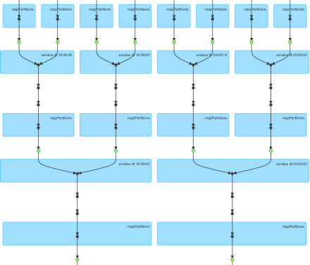
Figure 7: Progressive window widening in Apache Spark.

Code fragments illustrating an implementation of progressive window widening are provided below. The code snippets are also available as a https://gist.github.com/dtolpin/84158adce3e4218af06453771cae15f2GitHub Gist https://gist.github.com/dtolpin/84158adce3e4218af06453771cae15f2(http://tinyurl.com/hqugoyb). A visualization of a Spark Streaming job executing progressive window widening, as displayed by Apache Spark’s web UI, is shown in Figure 7.

Scala

The main loop is initialized with a stream of batches of unit size. Function detect is called at each level, applies a pattern recognition algorithm, and stores the result as a side effect.

⬇

(1 to config.depth).foldLeft((batches, 1)) {

case ((batch, batch_size), _) => {

// Generate sliding windows with half-window step

val windows = batches

.window(Seconds(2*window_size), Seconds(window_size))

.reduceByKey(_ ++ _)

// Apply data mining/pattern recognition algorithm

detect(windows)

widen(batch, batch_duration, config.max_length)

}

}

Functions widen and combine are defined as follows:

⬇

def combine[A](a: Vector[A], b: Vector[A], max_length: Int)

= {

val ab = a ++ b

if(ab.length > 2*max_length )

ab.patch(max_length, Seq(), ab.length - 2*max_length);

else

ab

}

def widen(_batches: DStream[(String, Vector[Syscall])],

_batch_duration: Int,

max_length: Int) = {

// Double batch duration

val batch_duration = _batch_duration*2

val batches = _batches

.window(Seconds(batch_duration), Seconds(batch_duration))

.reduceByKey(combine(_, _, max_length))

(batches, batch_duration)

}

Python

As in the Scala version, the main loop is initialized with a stream of batches of unit size. Function detect is called at each level, applies a pattern recognition algorithm, and stores the result as a side effect.

⬇

t = 1

for _ in range(ceil(log2(max_time))):

# Generate sliding windows with half-window step

windows = (batches

.window(2*t, t)

.reduce(lambda a, b: a + b))

# Apply data mining/pattern recognition algorithm

detect(windows)

# Double batch duration

t *= 2

batches = (batches

.window_size(t, t)

.reduce(lambda a, b: combine(a, b, max_length)))

Function combine is defined as follows:

⬇

def combine(a, b, max_length):

ab = a + b

if len(ab) - max_lenbgth > max_length:

ab[max_length:len(ab) - max_length] = []

return ab

References

- [1] Aggarwal, C.C., Han, J., Wang, J., Yu, P.S.: A framework for clustering evolving data streams. In: 29th International Conference on Very Large Data Bases. pp. 81–92. VLDB ’03, VLDB Endowment (2003)
- [2] Agrawal, D., Budak, C., Abbadi, A., Georgiou, T., Yan, X.: Databases in Networked Information Systems: 9th International Workshop, chap. Big Data in Online Social Networks: User Interaction Analysis to Model User Behavior in Social Networks, pp. 1–16. DNIS ’14, Springer International Publishing (2014)
- [3] de Aquino, A.L.L., Figueiredo, C.M.S., Nakamura, E.F., Buriol, L.S., Loureiro, A.A.F., Fernandes, A.O., Coelho, C.J.N.J.: Data stream based algorithms for wireless sensor network applications. In: IEEE 21st International Conference on Advanced Information Networking and Applications. pp. 869–876. AINA ’07, IEEE (2007)
- [4] Bifet, A., Gavaldà, R.: Learning from time-changing data with adaptive windowing. In: SIAM International Conference on Data Mining. SDM ’07, SIAM (2007)
- [5] Bifet, A., Pfahringer, B., Read, J., Holmes, G.: Efficient data stream classification via probabilistic adaptive windows. In: 28th Annual ACM Symposium on Applied Computing. pp. 801–806. SAC ’13, ACM (2013)
- [6] Gama, J.: A survey on learning from data streams: current and future trends. Progress in Artificial Intelligence 1(1), 45–55 (2012)
- [7] Golab, L., Özsu, M.T.: Issues in data stream management. SIGMOD Record 32(2), 5–14 (2003)
- [8] Gwadera, R., Atallah, M., Szpankowski, W.: Reliable detection of episodes in event sequences. In: Third IEEE International Conference on Data Mining. pp. 67–74. ICDM ’03, IEEE (2003)
- [9] He, B., Yang, M., Guo, Z., Chen, R., Su, B., Lin, W., Zhou, L.: Comet: Batched stream processing for data intensive distributed computing. In: 1st ACM Symposium on Cloud Computing. pp. 63–74. SoCC ’10, ACM (2010)
- [10] Mannila, H., Toivonen, H., Inkeri Verkamo, A.: Discovery of frequent episodes in event sequences. Data Mining and Knowledge Discovery 1(3), 259–289 (1997)
- [11] Varghese, S.M., Jacob, K.P.: Anomaly detection using system call sequence sets. Journal of Software 2(6), 14–21 (2007)
- [12] Warrender, C., Forrest, S., Pearlmutter, B.: Detecting intrusions using system calls: alternative data models. In: IEEE Symposium on Security and Privacy. pp. 133–145. SP ’99, IEEE (1999)
- [13] Yang, Y., Mao, G.: International Conference of Intelligence Computation and Evolutionary Computation, chap. A Self-Adaptive Sliding Window Technique for Mining Data Streams, pp. 689–697. ICEC ’12, Springer Berlin Heidelberg (2013)
- [14] Yolacan, E.N., Dy, J.G., Kaeli, D.R.: System call anomaly detection using multi-HMMs. In: IEEE Eighth International Conference on Software Security and Reliability-Companion. pp. 25–30. SERE-C ’14, IEEE (2014)
- [15] Zaharia, M., Chowdhury, M., Franklin, M.J., Shenker, S., Stoica, I.: Spark: Cluster computing with working sets. In: Proceedings of the 2Nd USENIX Conference on Hot Topics in Cloud Computing. pp. 10–10. HotCloud’10, USENIX Association, Berkeley, CA, USA (2010)
- [16] Zaharia, M., Das, T., Li, H., Hunter, T., Shenker, S., Stoica, I.: Discretized streams: Fault-tolerant streaming computation at scale. In: Twenty-Fourth ACM Symposium on Operating Systems Principles. pp. 423–438. SOSP ’13, ACM (2013)
- [17] Zaharia, M., Das, T., Li, H., Shenker, S., Stoica, I.: Discretized streams: An efficient and fault-tolerant model for stream processing on large clusters. In: 4th USENIX Conference on Hot Topics in Cloud Computing. pp. 10–15. HotCloud’12, USENIX Association (2012)
- [18] Zhang, D., Li, J., Zhang, Z., Wang, W., Guo, L.: Advances in Web-Age Information Management: 5th International Conference, chap. Dynamic Adjustment of Sliding Windows over Data Streams, pp. 24–33. WAIM ’04, Springer Berlin Heidelberg (2004)