Evolution operators in conformal field theories and conformal mappings:
the entanglement Hamiltonian, the sine-square deformation, and others

Abstract

By making use of conformal mapping, we construct various time-evolution operators in (1+1) dimensional conformal field theories (CFTs), which take the form $\int dx\,f(x)\mathcal{H}(x)$, where $\mathcal{H}(x)$ is the Hamiltonian density of the CFT, and $f(x)$ is an envelope function. Examples of such deformed evolution operators include the entanglement Hamiltonian, and the so-called sine-square deformation of the CFT. Within our construction, the spectrum and the (finite-size) scaling of the level spacing of the deformed evolution operator are known exactly. Based on our construction, we also propose a regularized version of the sine-square deformation, which, in contrast to the original sine-square deformation, has the spectrum of the CFT defined on a spatial circle of finite circumference $L$, and for which the level spacing scales as $1/L^{2}$, once the circumference of the circle and the regularization parameter are suitably adjusted.

I Introduction

Many classical statistical mechanical systems and quantum many-body systems at criticality enjoy conformal invariance – invariance under scale as well as special conformal transformations. Combined with translations and spatial rotations (or spacetime Lorentz boosts), they are invariant under the conformal group. That critical systems are conformally invariant can be exploited to put some constraints on the operator content of the critical theory. Such constraints are most restrictive and powerful in 2 or (1+1) dimensions, and in some cases can fully specifyCardy (1986) the critical theory.

In this work, we consider various kinds of ”deformations” of (1+1) dimensional conformal field theories (CFTs). By ”deformation” we mean the following. Let $\mathcal{H}(x)$ be the Hamiltonian density of a CFT where $x$ is the spatial coordinate. Then, the ordinary time-evolution is generated by

$$H=\int\,dx\,\mathcal{H}(x).$$ (1)

We ”deform” this Hamiltonian by introducing an ”envelope function” $f(x)$ as

$$H[f]=\int dx\,f(x)\,\mathcal{H}(x).$$ (2)

Similarly, suppose we have a lattice model, which is critical and described by a CFT. Schematically, its Hamiltonian is given by

$$H =\sum_{i}h_{i,i+1}$$ (3)

where $h_{i,i+1}$ is the lattice analogue of the Hamiltonian density. (We have restricted ourselves to the case of nearest-neighbor interactions, and neglected for simplicity further neighbor interactions. The lattice here can be periodic, infinite, or even open, but, we are interested in the Hamiltonian density.) We ”deform” this lattice Hamiltonian by introducing an ”envelope” function $f(x)$ as

$$H[f] =\sum_{i}f\left(\frac{{x_{i}+x_{i+1}}}{2}\right)h_{i,i+1}.$$ (4)

There are various problems that fit into the above class of deformations. For example, let us consider the ground state $|\Psi\rangle$ of a CFT defined on infinite one-dimensional space, and then define the reduced density matrix $\rho_{A}$ associated with a region $x\in(-R,R)$ by $\rho_{A}=\mathrm{Tr}_{B}\,|\Psi\rangle\langle\Psi|$, where the partial trace $\mathrm{Tr}_{B}$ is taken over the all degrees of freedom associated with the region outside of the interval $(-R,R)$. Then, the entanglement Hamiltonian $H_{E}$, defined by $\rho_{A}=\exp(-H_{E}),$ is of the form (2) where the envelope function is

$$f(x)=\frac{{R^{2}-x^{2}}}{2R},\quad x\in(-R,R),$$ (5)

and $f(x)=0$ otherwise, Hislop and Longo (1982); Haag (1992); Casini et al. (2011); Cardy ; Cho et al. (2016) i.e.,

$$H_{E}=\int^{R}_{-R}dx\,\frac{R^{2}-x^{2}}{2R}\mathcal{H}(x).$$ (6)

Another example is the so-called sine-square deformation (SSD) of quantum many-body Hamiltonians in (1+1) dimensions. Gendiar et al. (2009, 2010); Hikihara and Nishino (2011); Gendiar et al. (2011); Shibata and Hotta (2011); Maruyama et al. (2011); Katsura (2011, 2012); Hotta and Shibata (2012); Hotta et al. (2013); Okunishi and Katsura (2015); Tada (2015); Ishibashi and Tada (2015, 2016) In the SSD, one chooses the envelope function as

$$f(x)=\sin^{2}\frac{{\pi x}}{L},\quad x\in(0,L),$$ (7)

and $f(x)=0$ otherwise. It was discovered that, for CFTs, the ground state of the SSD Hamiltonian is identical to the ground state of the CFT defined on an infinite one-dimensional space. This has practical implications as the SSD Hamiltonian allows us to study the CFT in the thermodynamic limit by studying a finite system of length $L$ (in numerical simulations, say).

There are various other examples. For example, yet another context where such a deformation has been discussed is the quantum energy inequalities. Flanagan (1997)

Obviously, there are infinitely many ways to deform CFTs in this way. As an attempt to find a systematic and controlled construction of such deformations, we will make use of conformal mapping. Our construction can be described as follows: (i) We start from a reference (1+1)-dimensional spacetime, parameterized by a complex coordinate which is denoted in the following by $w$, and an evolution operator $\tilde{H}$. (ii) We next pick a suitable conformal map which maps the reference space-time (coordinate $w$) to the “target” spacetime, parameterized by a complex coordinate which we denote in the following by $z$. The conformal map maps the set of trajectories generated by $\tilde{H}$ (determined by the Killing vectors) in the reference spacetime to some (potentially complicated) trajectories in the complex $z$-plane. (iii) Finally, we transform $\tilde{H}$ and express it in terms of the energy-momentum tensor on the complex $z$-plane. If we choose the reference evolution $\tilde{H}$ to be something simple, by construction, the spectrum of the deformed Hamiltonian is known exactly, and so is its level spacing as a function of the parameters on which the conformal map depends (e.g., the system size). Put differently, in our construction we deal with the set of envelope functions, which we can “undo” by choosing a suitable conformal map.

The construction described above has been used, for example, to obtain the entanglement Hamiltonian in a number of cases. Peschel and Truong (1987); Cardy ; Cho et al. (2016) In this paper, by making use of conformal mapping, we describe various deformations of the CFT with various envelope functions, and also discuss the finite size scaling of their spectra. As a particular example, we obtain a “regularized version” of the SSD. The regularized SSD is closed related to the entanglement Hamiltonian (defined for a finite interval), in that the entanglement Hamiltonian and the regularized SSD can be obtained from the same conformal mapping. However, the direction of the evolutions generated by them are orthogonal to each other. (In the fluid dynamics language, the flows generated by these two evolution operators correspond to the equipotential lines and the streamlines, respectively.)

As compared to the original SSD, the regularized SSD has the following properties: The spectrum of the regularized SSD Hamiltonian matches the spectrum of a CFT with periodic boundary conditions (PBC). However, the level spacing of the regularized SSD Hamiltonian shows $(1/\mbox{length})^{2}$ scaling, as opposed to the familiar $(1/\mbox{length})$ scaling of a CFT with PBC. (To be more precise, the length here means the length in the complex plane – in the actual Hamiltonian, one needs to scale simultaneously both, the size of the system and the regularization parameter.)

On the contrary, the spectrum of the original SSD Hamiltonian is known to possess a continuous spectrum (in the continuum limit and at criticality). For this reason, it is rather subtle to discuss the scaling of the finite size spectrum of the SSD Hamiltonian on a lattice. Nevertheless, it has been shown numerically that the spectrum of the SSD Hamiltonian on a finite lattice shows $(1/\mbox{length})^{2}$ scaling. (Once again, this should be contrasted with the ordinary $(1/\mbox{{length}})$ scaling of ordinary CFT put on a finite cylinder. ) The regularized SSD does not have such subtle issues. The $(1/\mbox{length})^{2}$ scaling of the regularized SSD may shed some light on the scaling of the original SSD on a lattice, by taking the limit where the regularization parameter goes to zero.

By using the same idea, we also generated other deformations of CFTs. For example, we obtain the ”square root” deformation of CFTs, defined by the envelope function

$$f(x)=\sqrt{(R-x)(R+x)}$$ (8)

for $x\in(-R,R)$ and $f(x)=0$ otherwise (see Eq. (57)). We will show that the level spacing of the deformed evolution operator with the envelope function (8) does not depend on $R$. This deformation was previously discussed in the context of quantum information transport in quantum spin chains. In particular, so-called ‘perfect state transfer’ can be achieved in the XX model with inhomogeneous nearest neighbor couplings which are modulated according to the envelope function (8). Christandl et al. (2004); Albanese et al. (2004); Christandl et al. (2005); Kay (2009)

II Single vortex

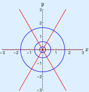
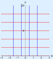
Figure 1: Conformal map $w=\log z.$

We will consider conformal maps from the Euclidean spacetime to another (“target”) spacetime. The “target” spacetime is parameterized by the complex coordinate $(z,\bar{z})$, and we write the real and imaginary parts of $z$ as

$$z=x+iy.$$ (9)

The coordinate of the “reference” spacetime is denoted by $(w,\bar{w})$, and we write the real and imaginary parts of $w$ as

$$w=u+iv.$$ (10)

As a warm up, we start by illustrating our strategy by taking the well-known example of the radial and angular quantization of CFTs in the complex plane. Consider the conformal mapping

$$w(z)=\log z$$ (11)

which maps the entire complex $z$-plane (“target” spacetime) into an infinitely long cylinder ($w$-coordinates; “reference spacetime”). This conformal map also transforms an annulus in the $z$-plane into a finite cylinder in the $w$-plane. In the following, we will consider a ‘flow’, or ‘time-evolution’ along the $u$ or the $v$ direction in the “reference” spacetime. We then consider the corresponding evolution in the “target” spacetime by ‘mapping back’ the evolution operator from the “reference” space time into the $z$-plane.

II.1 Radial flow (”radial quantization”)

The radial flow in the $z$-plane is mapped onto a ”straight” flow in the $w$-plane (flow along the $u$-direction). This simple evolution is generated by the evolution operator in the $u$-direction,

$$\tilde{H}=\int_{0}^{2\pi}dv\,\tilde{T}_{uu}(u_{0},v),$$ (12)

where $\tilde{T}_{uu}$ is the $uu$ component of the stress (energy-momentum) tensor, and we choose a particular “time” $u=u_{0}$ to define the evolution operator. This evolution operator is the Hamiltonian of a CFT on a circle of circumference $2\pi$. Since it is defined on a finite space, it has a discrete spectrum.

Mapping back to the $z$-plane, $\tilde{H}$ can be expressed in terms of the dilatation operator (a Virasoro generator) in the plane as

$$\frac{\tilde{H}}{2\pi}=L_{0}+\bar{{L}}_{0}-\frac{{c}}{24}$$ (13)

where $c$ is the central charge and $L_{0}$ and $\bar{L}_{0}$ are given by

$$L_{0}=\frac{{1}}{2\pi i}\oint dz\>z\>T(z),\quad\bar{L}_{0}=\frac{{-1}}{2\pi i}\oint d\bar{{z}}\>\bar{{z}}\>\bar{{T}}(\bar{{z}}).$$ (14)

The dilatation operator generates translations in the radial direction in the complex plane. This is the well-known radial quantization.

For later use, let us consider polar coordinates $(r,\theta)$ in the $z$-plane defined by

$$z=re^{i\theta}.$$ (15)

From the tensorial transformation law of the energy-momentum tensor,

$$T_{ij}=\tilde{T}_{\mu\nu}\frac{\partial u^{\mu}}{\partial x^{i}}\frac{\partial u^{\nu}}{\partial x^{j}},$$ (16)

$\tilde{T}_{uu}$ can be expressed as

$$T_{rr}(r,\theta)=\tilde{T}_{uu}\frac{\partial u}{\partial r}\frac{\partial u}{\partial r}=\frac{1}{r^{2}}\tilde{T}_{uu}(u,v)$$ (17)

(up to the Schwartzian derivative term). Hence, $\tilde{H}$ can also be expressed as

$$\tilde{H}=r^{2}_{0}\int_{0}^{2\pi}dv\,T_{rr}(r_{0},\theta)=r^{2}_{0}\int_{0}^{2\pi}d\theta\,T_{rr}(r_{0},\theta),$$ (18)

where $r_{0}$ is defined by $u_{0}=\log r_{0}$.

Since the circumference of the circle in the $z$-plane is $L:=2\pi r_{0},$ it is natural to introduce

$$\theta=\frac{2\pi}{L}s,\quad s\in[0,L],\quad L=2\pi r_{0}.$$ (19)

Then, $\tilde{H}$ can be written as

$$\tilde{H}=\frac{L}{2\pi}\int^{L}_{0}ds\,T_{rr}\left(\frac{L}{2\pi},\frac{2\pi s}{L}\right).$$ (20)

Comparing with Eq. (13), the spectrum of the operator

$$\int^{L}_{0}ds\,T_{rr}\left(\frac{L}{2\pi},\frac{2\pi s}{L}\right)$$ (21)

scales as $1/L$, and hence this operator can be consideredCardy (1984) as the Hamiltonian of a CFT defined on a circle of circumference $L$.

II.2 Angular flow (”Rindler Hamiltonian”)

The conformal transformation in Eq. (11) also maps the angular flow in the $z$-plane into the ”straight” flow along the $v$-direction in the $w$-plane. This simple time-evolution is generated by the evolution operator in $v$ direction

$$\tilde{H}=\int_{-\infty}^{+\infty}du\>\tilde{T}_{vv}(u,v).$$ (22)

We next transform this evolution operator back into the $z$-plane. Using the tensorial transformation law (16), the energy-momentum tensor on the cylinder and in the plane are related by

$$T_{yy} =\frac{1}{(x^{2}+y^{2})^{2}}\left[y^{2}\tilde{T}_{uu}+(xy)^{2}(\tilde{T}_{uv}+\tilde{T}_{vu})+x^{2}\tilde{T}_{vv}\right].$$ (23)

In particular, when $y=0$ we have the relationship $T_{yy}=x^{-2}\tilde{T}_{vv},$ and hence when expressed in the $z$-plane, $\tilde{H}$ is given by

$$\tilde{H} =\int du\tilde{T}_{vv}=\int^{\infty}_{0}dx\,xT_{yy}.$$ (24)

This is the Hamiltonian in Rindler spacetime. The Rindler Hamiltonian Eq. (24) generates the angular flow (the Lorentz-boost in Minkowski signature), and corresponds to “angular quantization” in the $z$-plane. It is also nothing but the entanglement Hamiltonian of the reduced density matrix associated to the semi-infinite interval $x\in(0,\infty)$ (where we consider the ground state $|\Psi\rangle$ of a CFT defined on infinite one-dimensional space, and then take the partial trace over all degrees of freedom for $x\in(-\infty,0)$.) - Since the entanglement or Rindler Hamiltonian (or Lorentz-boost) in Eq. (24) is equal to the Hamiltonian Eq. (22) of the CFT defined on an infinite space, its spectrum is continuous.

III Vortex-anti-vortex pair

Table 1: Conformal map $w=\log(z+1)/(z-1).$

In this section, we consider the conformal map

$$w(z)=\log(z+R)-\log(z-R),$$ (25)

with inverse $z(w)=$ $R\coth(w/2)$. This maps the entire complex $z$-plane into an infinitely long cylinder. The coordinate $v$ in the “reference” spacetime (coordinates $w$) is periodic with period $=2\pi$. This conformal map can be thought of as describing the complex potential of a flow which consists of a source with unit strength located at $z=-R$, represented by the complex potential $\log(z+R)$, and a sink with the same strength located at $z=+R$.

Taking the limit $R/z\to 0$, the vortex-anti-vortex pair reduces to a dipole,

$$\log\frac{{z+R}}{z-R} \sim\frac{{2R}}{z}.$$ (26)

It is also convenient to consider a pair of a vortex of strength $k$ and an anti-vortex of strength $-k$. Then, by letting $R\to 0$ and $k\to\infty$ such that $2kR$ is finite,

$$w(z)=k\log\frac{{z+R}}{z-R} \sim\frac{{2Rk}}{z}.$$ (27)

This is the complex potential due to a dipole, i.e., the combination of a source and sink of equal strengths separated by a very small distance. The quantity $2kR$ is the dipole moment. - Note that the inverse of the left equation in Eq. (27) reads $z(w)=R\coth(w/2k)$, which shows that the period of $v$ in the “reference” spacetime tends to infinity in the dipolar limit, $k\to\infty$. This is consistent with the fact that ‘dipolar map’ $w=1/z$ maps the entire complex plane into itself. (See also Section IV.)

III.1 $v$-evolution: Entanglement Hamiltonian

As in the simple exercise we did in Sec. II, we now consider two kinds of time-evolutions associated to the conformal map (25).

Let us first take $v$ as time, and consider the evolution operator at $v=v_{0}=\pi$,

$$\tilde{H}=\int_{-\log[(2R-\epsilon)/\epsilon)}^{+\log[(2R-\epsilon)/\epsilon]}du\,\ \tilde{T}_{vv}(u,v_{0}=\pi).$$ (28)

Here, we have cut off the integral over $u$ by introducing an UV cutoff $\epsilon>0$ in position space $x$ (so that $-R+\epsilon<x<+R-\epsilon$).

The (time-)evolution operator in (28) generates the evolution along the constant $u$-trajectories. In the fluid dynamic terminology, these are equipotential lines and are given in the $z$-plane by

$$[x\pm R\,\coth(u)]^{2}+y^{2}=\frac{{R^{2}}}{\sinh^{2}(u)}.$$ (29)

Thus, the constant $u$ trajectories are, for different values of $u$, circles having centers at $(x,y)=(\pm R\coth(u),0)$ and radii equal to $R/|\sinh(u)|$. (Compare TABLE 1.)

The evolution operator (28) can be now mapped into the $z$-plane. Focusing on $y=0$, $\tilde{T}_{vv}$ is transformed as

$$T_{yy} =\tilde{T}_{vv}\left(\frac{\partial v}{\partial y}\right)^{2}=\tilde{T}_{vv}\left[\frac{2R}{(x-R)(x+R)}\right]^{2},$$ (30)

and hence $\tilde{H}$, when mapped into the $z$-plane, reads

$$\tilde{H}=\int_{-R+\epsilon}^{+R-\epsilon}dx\frac{{(x-R)(x+R)}}{2R}T_{yy}.$$ (31)

This is the entanglement Hamiltonian obtained from a CFT defined on an infinite line, after tracing out degrees of freedom living outside of the finite interval $x\in[-R,R]$.Hislop and Longo (1982); Haag (1992); Casini et al. (2011); Cardy ; Cho et al. (2016)

III.2 $u$-evolution: “Regularized” SSD

Let us now move on to consider the evolution operator along the $u$-direction in $w$-space which is given by

$$\tilde{H}=\int^{\pi}_{0}dv\,\tilde{T}_{uu}(u_{0},v)$$ (32)

where we fix $u=u_{0}$. The constant-$v$ trajectories under this evolution, which are ‘streamlines’ in the fluid dynamics language, are given in the $z$-plane by

$$x^{2}+[y+R\cot(v)]^{2}=\frac{{R^{2}}}{\sin^{2}(v)}.$$ (33)

For different values of $v$, these are circles with centers at $(0,-R\cot(v))$, and radii $R/|\sin(v)|$. These circles pass through $(\pm R,0)$. - See TABLE 1.

Turning now to the constant-$u$ “time”-slices (the Cauchy surfaces for the current choice of “time”-evolution), we see from Eq. (29) that their $(x,y)$-coordinates in the $z$-plane satisfy, for a fixed $u=u_{0}$,

$$\left(x+\frac{{\cosh u_{0}}}{\sinh u_{0}}R\right)^{2}+y^{2}=\frac{{R^{2}}}{(\sinh u_{0})^{2}}.$$ (34)

These are circles of radius $r_{0}$ and circumference $L$, where

$$r_{0}:=\frac{{R}}{\sinh u_{0}},\quad{\rm and}\ \ L=2\pi r_{0}.$$ (35)

The evolution operator (32), defined at $u=u_{0}$, acts on quantum states defined on the circle.

Making use of the transformation law of the energy-momentum tensor,

$$T_{rr}=\tilde{T}_{uu}\left(\frac{\partial u}{\partial r}\right)^{2}=\tilde{T}_{uu}\frac{1}{r_{0}^{2}}\left(\frac{\sinh u_{0}}{\cos\theta+\cosh u_{0}}\right)^{2},$$ (36)

$\tilde{H}$ can be mapped into the $z$-plane and can be written as

$$\tilde{H} =r_{0}^{2}\int^{2\pi}_{0}d\theta\,\frac{\cos\theta+\cosh u_{0}}{\sinh u_{0}}\,T_{rr}(r,\theta).$$ (37)

By further introducing

$$\theta=\frac{2\pi}{L}s,\quad s\in[0,L],$$ (38)

$\tilde{H}$ is written as

$$\tilde{H} =\frac{L}{2\pi}\frac{1}{\sinh u_{0}}\int^{L}_{0}ds\,$$

$$\quad\times\left(\cos\frac{2\pi s}{L}+\cosh u_{0}\right)T_{rr}\left(r=\frac{L}{2\pi},\theta=\frac{2\pi s}{L}\right).$$ (39)

From the discussion in the paragraph containing Eq. (21), the operator $\int^{L}_{0}ds\,T_{rr}\left(L/2\pi,2\pi s/L\right)$ is the Hamiltonian of a CFT defined on a circle of circumference $L$. Thus, the part of $\tilde{H}$ which we call $H_{\mathrm{rSSD}}$, defined by

$$H_{\mathrm{rSSD}}=\int^{L}_{0}ds\left(\cos\frac{2\pi s}{L}+\cosh u_{0}\right)T_{rr}\left(\frac{L}{2\pi},\frac{2\pi s}{L}\right),$$ (40)

is the ”deformed Hamiltonian” with the envelope function $\left(\cos(2\pi s/L)+\cosh u_{0}\right)$. Because of the presence of the term $\cosh u_{0}$, this deformation is different from the ordinary SSD, and can be regarded as a ”regularized” version of the SSD. The limit $u_{0}\to 0$ corresponds to the ordinary SSD, which for fixed $L$, or equivalently for fixed $r_{0}$, corresponds to $R\to 0$. (See Eq. (35).) As discussed in the paragraph containing Eq. (27) this is the dipolar limit.

By construction, when $u_{0}\neq$0, the spectrum of the $u$-evolution operator is the spectrum of a CFT defined on a finite circle (i.e., with PBC), which is discrete. This should be contrasted with the ordinary SSD, for which the spectrum of the evolution operator is a continuum.

Finite Size Scaling

We now turn to the finite-size scaling of the spectrum of the regularized SSD evolution operator, Eq. (40). (Once again, in the SSD limit $u_{0}\to 0$, the spectrum is continuous, and hence there is no finite size scaling to discuss.) We can in principle discuss the following two kinds of finite-size scaling behaviors.

First, we fix $u_{0}$ and change the distance $R$ between the two monopoles which controls the (spatial) size of the system. Since $\tilde{H}$ has a level spacing of order one, recalling (35), the level spacing of $H_{\mathrm{rSSD}}=(2\pi\sinh u_{0}/L)\tilde{H}$ scales as

$$\sim\frac{\sinh u_{0}}{L}={1\over 2\pi}\frac{(\sinh u_{0})^{2}}{R}\sim\frac{1}{R}.$$ (41)

Since $R$ is proportional to $L$ when $u_{0}$ is fixed, this means $1/L$ scaling.

On the other hand, we can fix $R$ and change $u_{0}$ which, due to (35), also controls the size $L$ of the system. In this case, the level spacing scales as

$$\sim\frac{\sinh u_{0}}{L}={1\over 2\pi}\frac{(\sinh u_{0})^{2}}{R}\sim\frac{1}{L^{2}}.$$ (42)

This should be contrasted with the regular $1/L$ scaling of CFTs put on a finite spatial circle of circumference $L$. It should also be noted that for the original SSD, previous numerical studies reported $1/L^{2}$ scaling. Gendiar et al. (2010); Hotta et al. (2013) The $1/L^{2}$ scaling of the regularized SSD may be related to this observation. Finally, as we will discuss momentarily, for the original SSD the spectrum consists of a continuum, when we consider the continuum field theory (CFT) formulation of the system, and hence there is no finite size scaling to discuss.

The Dipolar Limit

Let us now consider the dipolar limit $R\to 0$. In the dipolar limit, the spacetime cylinder in $w$-space shrinks as it is bounded in the $u$-direction by the cut off $\pm\log[(2R-\epsilon)/\epsilon]$. - See Eq. (28). (Note that in the section containing Eq. (28), we discussed the entanglement Hamiltonian where $u$ represented the “spatial” coordinate, and $v$ the (imaginary time) “temporal” coordinate. In contrast, in the present section, we have chosen the $u$-direction as our (imaginary time) “temporal”, and the $v$-direction as our ”spatial” coordinate.) Thus, in the limit $R\to\epsilon$, the (“temporal”) $u$-direction shrinks to zero. Hence, the ”modular parameter” of the CFT, which depends on the aspect ratio of space and (imaginary) time directions, is given by

$$\mbox{(total space length)}/\mbox{(total time length)}\to\infty.$$ (43)

This can be interpreted as achieving the infinite size limit, as noted by Ishibashi and Tada. Ishibashi and Tada (2015, 2016)

Before closing this section, let us discuss the special case $u=0$. This means that we consider the evolution in the $z$-plane right on the imaginary axis, $x=0$, rather than on a finite circle that we considered when $u\neq 0$. Hence, we consider the evolution (flow) that brings the infinite line to a point (eventually, at asymptotically long times). - See TABLE 1. The evolution operator $\tilde{H}=\int dv\tilde{T}_{uu}(u=0,v)$ is mapped into

$$\tilde{H}=\int_{-\infty}^{+\infty}\,dy\,\ \frac{y^{2}+R^{2}}{2R}T_{xx}.$$ (44)

By construction, this Hamiltonian $\tilde{H}$ has a spectrum which is described by a CFT with PBC, although the system is defined on infinite one-dimensional space. In the dipolar limit, $R\ll y$, this yields

$$\tilde{H}=\frac{1}{2R}\int\,dy\frac{{1+(R/y)^{2}}}{y^{-2}}T_{xx}\sim\frac{{1}}{2R}\int\,dy\,y^{2}T_{xx}.$$ (45)

This evolution operator can be considered as derived from the decompactification limit of the SSD Hamiltonian: $\int_{0}^{L}\,dx\,\sin^{2}\frac{{\pi x}}{L}\mathcal{{H}\sim\int}dx\,x^{2}\mathcal{{H}}.$ Observe that while before taking the dipolar limit, the system is defined on the whole imaginary axis; the limit $R\to 0$ ”cuts” the imaginary axis into two halves, $y>0$ and $y<0$.

IV Dipolar map

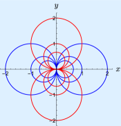
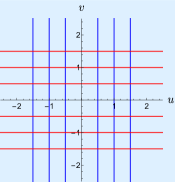
Figure 2: Conformal map $w=1/z$.

The conformal map

$$w=\frac{1}{z}$$ (46)

describes the dipolar flow, which maps the entire complex $z$-plane into the entire complex $w$-plane. As described in the paragraph containing Eq. (27), the corresponding flow can be obtained from a pair of a vortex and an anti-vortex, by taking the limit where their separation goes to zero. Here, we directly deal with the dipolar flow without taking the limit.

We will focus on the evolution in $u$-direction. Furthermore, we use the parametrization $u=1/(2r_{0})$. For $u=1/(2r_{0})$, Eq.(46) implies

$$\frac{{1}}{2r_{0}}=\frac{{x}}{x^{2}+y^{2}}\Rightarrow(x-r_{0})^{2}+y^{2}=r^{2}_{0}.$$ (47)

Thus, the constant $u$ trajectories are circles of radius $r_{0}$ centered at $(r_{0},0)$.

We consider the evolution operator in $w$-space given by

$$\tilde{H}=\int_{-\infty}^{+\infty}dv\,\ \tilde{T}_{uu}(u_{0},v),$$ (48)

and then map $\tilde{H}$ to the $z$-plane. In the $z$-plane, we work with the polar coordinate $(r,\theta)$ defined by

$$x-r_{0}=:r_{0}\cos\theta,\quad y=:r_{0}\sin\theta.$$ (49)

By transforming $\tilde{H}$, the evolution operator in the $r$ direction is generated by

$$\tilde{H} =4r_{0}^{3}\int^{2\pi}_{0}d\theta\cos^{2}(\theta/2)\,T_{rr}(r_{0},\theta).$$ (50)

Shifting the angular variable $\theta\equiv\phi+\pi$ for convenience, and introducing $L=2\pi r_{0}$ as well as $\phi\equiv 2\pi s/L$, this reads

$$\tilde{H} =4r_{0}^{3}\int^{2\pi}_{0}d\phi\sin^{2}(\phi/2)\,T_{rr}(r_{0},\theta)$$

$$=\frac{L^{2}}{\pi^{2}}\int^{L}_{0}ds\,\sin^{2}\frac{\pi s}{L}\,T_{rr}\left(\frac{L}{2\pi},\frac{2\pi s}{L}\right).$$ (51)

Thus, we have related $\tilde{H}$ to

$$H_{\mathrm{SSD}} =\int^{L}_{0}ds\,\sin^{2}\frac{\pi s}{L}\,T_{rr}\left(\frac{L}{2\pi},\frac{2\pi s}{L}\right).$$ (52)

By construction, we expect this SSD Hamiltonian has a CFT spectrum on the infinite line, although $H_{\mathrm{SSD}}$ is defined for a circle of circumference $L$. The prefactor $L^{2}$ relating $\tilde{H}$ and $H_{\mathrm{SSD}}$ is indicative of the $1/L^{2}$ scaling. However, since both, $H_{\mathrm{SSD}}$ as well as $\tilde{H}$ (defined on infinite space - see Eq. (48)) have a continuum spectrum, there is no finite size scaling that we can discuss for the level spacing.

V Inverse sine map

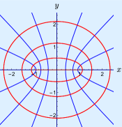
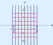
Figure 3: Conformal map $z=\sin(w)$.

As yet another conformal transformation, let us consider

$$z=R\sin w.$$ (53)

By this transformation, the infinite strip defined by $-\pi/2<u<\pi/2$ and $-\infty<v<+\infty$ is mapped onto the complex $z$-plane.

Consider the evolution operator in the $v$-direction. At “time” $v=v_{0}$ this reads

$$\tilde{H}=\int^{+\pi/2-\delta}_{-\pi/2+\delta}du\,\tilde{T}_{vv}(u,v_{0}),\qquad(\delta\to 0^{+}).$$ (54)

In the following, we focus on $y=0$, which translates into $v_{0}=0$. Then, $x$ and $u$ are related by $x/R=\sin u$.

In (54), the upper and lower limit of the integral should be suitably cut off. As $u$ ranges over the interval $(-\pi/2,+\pi/2)$, $x$ ranges over the interval $(-R,R)$. When $x$ is close to its upper limit, $x=R-\epsilon$ where $\epsilon\to 0^{+}$, which suggests

$$R-\epsilon=R\sin(\pi/2-\delta)=R(1-\delta^{2}/2+...),$$ (55)

and hence $\delta\sim\sqrt{{2\epsilon}/R}\to 0^{+}$. In terms of $\epsilon$, the evolution operator is then written as

$$\tilde{H}=\int_{-\pi/2+\sqrt{2\epsilon/R}}^{+\pi/2-\sqrt{{2\epsilon/R}}}du\,\tilde{T}_{vv}(u,v=0).$$ (56)

By mapping $\tilde{T}_{vv}(u,v)$ to $T_{yy}(x,y)$ we obtain

$$\tilde{H}=\int_{-R+\epsilon}^{+R-\epsilon}dx\,\sqrt{{R^{2}-x^{2}}}\,T_{yy}(x,y=0).$$ (57)

We call this evolution operator ”the square root deformation” (SRD). This evolution operator is somewhat similar to the entanglement Hamiltonian. However, this evolution brings (eventually, at asymptotically long times) the interval $x\in(-R,R)$ to to infinite space $x\in(-\infty,+\infty)$, unlike the entanglement Hamiltonian which takes the interval $(-R,R)$ to its compliment on the real axis. Note that, interestingly, by construction the spectrum of the square root deformation, Eq. (57), does not scale with $R$.

VI Numerics

In this section, we use specific lattice models, such as the s=1/2 XX quantum spin model, to study the deformed Hamiltonians. We have also checked numerically the transverse Ising model and the XXZ model, but the results for these models are qualitatively similar. We therefore focus here on the XX model.

The spin 1/2 XX model is defined by:

$$H=\sum_{i}\left(S_{i}^{x}S_{i+1}^{x}+S_{i}^{y}S_{i+1}^{y}\right)=\sum_{i}h_{i,i+1},$$ (58)

where $S^{x,y,z}_{i}$ is the spin 1/2 operator defined at site $i$ of a one-dimensional lattice. The finite-size spectra of the XX model, both for PBC and for open boundary conditions (OBC), are shown in Fig.  4. The low-energy part of these spectra are described by the $c=1$ compactified free boson theory. We will use these spectra as our reference when discussing the spectra of the deformed evolution operators.

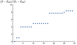
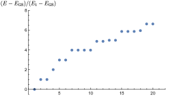
Figure 4: The finite size spectra of the XX model (18 sites) with PBC and OBC.

VI.1 SSD

Let us now consider the deformation of the XX model by the envelope function:

$$f(x)=\cos\frac{{2\pi x}}{L}+1$$ (59)

The resulting SSD Hamiltonian is given by

$$H_{\mathrm{{SSD}}}=\sum_{i=1}^{L}f(x_{i}+1/2)h_{i,i+1}$$ (60)

where we impose the PBC, $h_{L,L+1}=h_{L,1}$. For previous analytical studies of the SSD of the XX model, see Ref. Okunishi and Katsura, 2015.

In the continuum Hamiltonian, we expect that this model exhibits a continuum spectrum even when the system is put on a circle of finite circumference. The numerical, exact-diagonalization spectrum of the model shows a spectrum which does not compare well with the CFT spectrum, neither with PBC nor with OBC (Fig. 5), at least for the system sizes we studied.

On the other hand, finite size scaling analysis shows the level spacing scales as $\sim 1/L^{2}$ (Fig. 5). This finding agrees with a previous numerical study. Hotta et al. (2013)

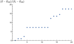
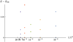
Figure 5: The finite size spectra of the XX model with the SSD (18 sites) and the finite size scaling analysis of its low-lying spectrum.

VI.2 Regularized SSD

Next, we turn to the regularized SSD. The regularized SSD deformation of the XX model is given by the envelope function

$$f(x)=\cos\frac{2\pi x}{L}+\sqrt{{1-R^{2}/L^{2}}}.$$ (61)

Here $R$ here is a parameter which serves as a regularization. The envelope function reduces to the SSD envelope function by taking the limit $R\to 0$. The resulting SSD Hamiltonian is given by

$$H_{\mathrm{{rSSD}}}=\sum_{i=1}^{L}f(x_{i}+1/2)h_{i,i+1}$$ (62)

where we impose the PBC, $h_{L,L+1}=h_{L,1}$.

In the continuum limit, we expect that this model exhibits the spectrum of a CFT defined on a spatial circle. The low-lying part of the numerical exact-diagonalization spectrum of the model (Fig. 6) compares reasonably with the expected spectrum of the CFT with PBC in Fig. 4.

As for the finite size scaling, we scale the system size as well as the second term in the enveloping function. From the finite size scaling analysis within continuum field theories, we expect the level spacing scales as $\sim 1/L^{2}$. The numerical analysis in Fig. 4 up to $L\sim 20$ sites, where we choose $R=20$, is in reasonable agreement with the expected $1/L^{2}$ scaling. On the other hand, we have checked that, if we choose a smaller value of $R$, $R\sim 1$, the low-lying spectrum does not look like the CFT with PBC.

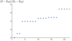
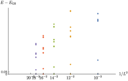
Figure 6: The finite size spectra of the XX model with the regularized SSD (18 sites) and the finite size scaling analysis of its low-lying spectrum. We chose $R=20.$

VI.3 Square root deformation (SRD)

Finally, the square root deformation of the XX model is given by the envelope function

$$f(x) =\sqrt{{(L/2)^{2}-(x-1/2-L/2)^{2}}}$$

$$=\sqrt{(x-1/2)(L-x+1/2)}.$$ (63)

Observe that we have a ”shift” by 1/2, which ensures $f(L+1/2)=0$. The resulting SRD Hamiltonian is given by

$$H_{\mathrm{{SRD}}}=\sum_{i=1}^{L}f(x_{i}+1/2)h_{i,i+1}$$ (64)

where $f(L+1/2)h_{L,L+1}=0$.

In the continuum limit, we expect that this model exhibits the spectrum of a CFT with boundary. The low-lying part of the numerical exact-diagonalization spectrum of the model (Fig. 7) compares very well with the spectrum of the XX model with OBC (Fig. 4). As for the level spacing, the finite size scaling analysis shows the level spacing scales as $\sim 1/L^{0}$ as expected. In fact, already from the very small system size ($L=4$), the low-lying spectrum of $H_{\mathrm{SRD}}$ (64) the finite size spectra of the XX model with OBC agrees surprisingly well (almost perfectly).

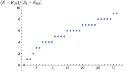
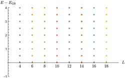
Figure 7: The finite size spectra of the XX model with the square root deformation (18 sites) and the finite size scaling analysis of its low-lying spectrum.

In fact, this deformation is quite peculiar. When applied to a non-interacting fermion system, it completely ”straightens” out the spectrum, and hence makes the spectrum perfectly relativistic, as analytically shown in Ref. Christandl et al., 2004.

VII Conclusion

Summarizing, we have constructed various deformed evolution operators of type (2). In particular, we have constructed a regularized version of the SSD. From our construction, it is also obvious that the regularized SSD Hamiltonian has a very close connection with the entanglement Hamiltonian; the evolution generated by the regularized SSD and the entanglement Hamiltonian are orthogonal to each other.

We have also studied the scaling of the level spacing of the spectra of the deformed evolution operators. The regularized SSD shows $1/L^{2}$ scaling as opposed to (i) the regular $1/L$ scaling of CFTs put on a finite spatial circle of circumference $L$ and (ii) the scaling of the spectrum of the original SSD Hamiltonian. For the latter, within the continuum field theory description, the spectrum consists of a continuum (and hence there is no scaling to be discussed for the level spacing). When the SSD Hamiltonians are studied on discrete one-dimensional lattices, $1/L^{2}$ level spacing has been observed, which seems closely related to the scaling of the regularized SSD.

Generalization to conformal maps (e.g.Rastelli and Zwiebach (2001), $z=(2/\pi)\mathrm{arctan}\,w$ ) other than those we considered in this paper should be straightforward. To give a broader perspective, it is worth pointing out that our construction, namely, the construction of the deformed evolution operator on the complex $z$-plane from some reference evolution operator on the $w$-plane (cylinder or strip), is closely related to the classification scheme of conformal vacua Birrell and Davies (1984); Candelas and Dowker (1979) in curved spacetime. In that classification, we are interested in a curved spacetime $M$, which is conformally mapped into the flat spacetime $\tilde{M}$. We suppose that $\Sigma$, a global Cauchy hypersurface of $M$, is mapped under the conformal transformation to a global Cauchy hypersurface $\tilde{\Sigma}$ of $\tilde{M}$. Then, for a timelike conformal Killing vector field in $\tilde{M}$, there exists a global timelike conformal Killing vector field in $M$. Thus, we can classify the conformal vacua defined with respect to the latter conformal Killing vector field by reference to the vacua defined in $\tilde{M}$. Birrell and Davies (1984) In Ref. Candelas and Dowker, 1979, various (1+1) dimensional spacetimes are conformally mapped into the Einstein static universe (which can be represented as a spacetime cylinder.)

Taking the $z$-plane (the $w$-space) as $M$ ($\tilde{M}$), the only minor difference is that here we have considered Euclidean conformal field theories, while in Ref. Candelas and Dowker, 1979 conformal field theories in curved spacetime with Minkowski signature are studied. At any rate, the global considerations as well as the classification scheme developed in Ref. Candelas and Dowker, 1979 can all be applied to the set of deformed evolution operators discussed in this paper.

Note added: Upon completion of this work, we became aware of the recent preprint Ref. Okunishi, 2016, in which the regularized SSD is also studied.