Coulomb field in a constant electromagnetic background

Abstract

Nonlinear Maxwell equations are written up to the third-power deviations from a constant-field background, valid within any local nonlinear electrodynamics including QED with a Euler-Heisenberg (EH) effective Lagrangian. The linear electric response to an imposed static finite-sized charge is found in the vacuum filled by an arbitrary combination of constant and homogeneous electric and magnetic fields. The modified Coulomb field and corrections to the total charge and to the charge density are given in terms of derivatives of the effective Lagrangian with respect to the field invariants. These are specialized for the EH Lagrangian.

1 Introduction

The large values of electromagnetic fields, close to or larger than $\frac{m^{2}}{e}=4.4\cdot 10^{13}G=1.6\cdot 10^{16}V/cm$, are present not only in astrophysical objects, such as pulsars, magnetars and quark stars, but also in the close vicinities of elementary particles as produced by their charges, magnetic and electric dipole moments. (For instance, the magnetic field of the neutron at the edge of its electromagnetic radius makes up the value of about $10^{16}G$, characteristic of magnetars.) This fact is encouraging interest in nonlinear electrodynamics that accounts for the effects of interaction between electromagnetic fields when at least one of them is large. These are, for instance, linear, quadratic and cubic responses of the vacuum, that include large “background” or “external” electromagnetic fields, to probe fields of, say, the ones produced by charges and currents. Another example of nonlinear effects is the correction to the magnetic and electric dipole moments of elementary particles and resonances owing to their self-coupling.

Another circumstance that has been fueling interest in the effects of quantum electrodynamics, this time within the framework of (2+1)-dimensional space-time, is the problem of Coulomb impurities in graphene; see the most recent review in Ref [1] and also the recent paper [2]. The point is that the effective coupling in that theory is much larger, and, correspondingly, the values of the fields optimal for nonlinearity are much smaller than in the (3+1)-dimensional QED.

Among the possible background fields most handy are those that admit an exact solution to the Dirac equation for the electron, which enables explicitly exploiting the Furry picture in order to take the background exactly while calculating the response functions – the polarization operators of different ranks. These are the plane-wave field (see the review [3]), the Coulomb field (dealt with in Ref. [4]), and the constant homogeneous field [5, 6]. However, only the latter admits, strictly speaking, a treatment with the use of a local electromagnetic action. The local approach, thanks to its relative simplicity, proved to be very fruitful in revealing special nonlinear effects [7]. These include the consequences of nonlinearity of quantum electrodynamics stemming from the quantum phenomenon of virtual electron-positron pairs creation by a photon, the pairs interacting with an electromagnetic field before their mutual annihilation. The corresponding interaction between electromagnetic fields is included at the local level by appealing to the Euler-Heisenberg effective action either at the one-loop [8, 9, 10] or two-loop [11] level giving rise to a modification of the classical Maxwell equations. Among the other, intrinsically nonlinear local classical theories of electromagnetism, the most popular is the geometrically elegant Born-Infeld model [12] , also arisen in the low-energy limit out of the string theory in the electromagnetic sector [13]. Its extensions [14, 15] are also in use. All these models are automatically included in our local treatment.

Many effects of nonlinear electrodynamics were considered before. The ones for which the three-photon diagram in an external magnetic field is responsible are the photon splitting [16] and the quadratic in the electric charge magnetoelectric effect when the charge becomes a magnetic dipole [17]. The cubic effect for which the light-by-light four-photon diagram is responsible was considered [18] without a background to produce nonlinear corrections to electric and magnetic dipoles and other sources. In the present paper, we are studying solutions of the Maxwell equations linearized above the background, which is an arbitrary combination of space- and time-independent electric and magnetic fields. We concentrate on finding the electric response to the applied field of a static charge; in other words, we are looking for the Coulomb field modified by the presence of this complex background. Previously, the Coulomb correction was considered (also beyond the local regime) in the external magnetic field taken alone [19, 20, 21, 22, 23]. In the combined field considered here, also a magnetic response to the electrostatic source exists. The preliminary study of it has indicated the possible presence of a solution carrying a magnetic monopole [24] in the simplifying case of a small background and parallel background fields. However, we postpone the detailed description of the magnetic response in the general case free of these restrictions to a forthcoming paper.

In Sec. 2, supported by Appendix A, we present the derivation of nonlinear Maxwell equations with background fields including quadratic and cubic nonlinearities. In Sec. 2, we find the linear correction to the Coulomb field in a constant background. In Subsec. 3.2.1, we describe the current induced by the background fields and by the probe field of an electric charge of finite radius, and we find the nonvanishing correction to the total charge. In Subsec. 3.2.2, we study the solutions for the modified Coulomb field calculated in Appendix B by using the projector method that separates the solutions subject to the first pair of Maxwell equations. The special cases of parallel external fields and the corresponding scalar potential are considered in Secs. 3.2.3 and 3.2.4. In Sec. 4, we concentrate on some realizations of the considered effects stemming from the use of the Euler-Heisenberg Lagrangian as a quantum source of nonlinearity. We consider small- and large-field limits, especially an extension of the effect of screening of the charge by strong magnetic field [19, 20, 21, 22, 23] to the case where a smaller electric field is also present. The results are finally discussed in the conclusions.

2 Nonlinear Maxwell equations at the infrared regime

2.1 Maxwell equations for arbitrary strong fields

The equations of motion of a nonlinear Maxwell theory, which incorporates the contribution of an effective field theory into its formulation, are extracted from the action,

$$S\left[A\right]=S_{\mathrm{Max}}\left[A\right]+S_{\mathrm{int}}\left[A\right]+\Gamma\left[A\right]\,,$$

$$S_{\mathrm{Max}}\left[A\right]=-\int\mathfrak{F}\left(x\right)d^{4}x\,,\ \ S_{\mathrm{int}}\left[A\right]=-\int J_{\mu}\left(x\right)A^{\mu}\left(x\right)d^{4}x\,,\ \ \Gamma\left[A\right]=\int\mathfrak{L}\left(x\right)d^{4}x\,,$$ (1)

in the form of Euler-Lagrange equations $\delta S\left[A\right]/\delta A^{\mu}\left(x\right)$,

$$\partial^{\nu}F_{\nu\mu}\left(x\right)+\frac{\delta\Gamma\left[A\right]}{\delta A^{\mu}\left(x\right)}=J_{\mu}\left(x\right)\,,$$ (2)

where $A^{\mu}\left(x\right)$ are electromagnetic potentials, $S_{\mathrm{Max}}\left[A\right]$ is the free Maxwell action, $S_{\mathrm{int}}\left[A\right]$ is the interaction with a classical current $J_{\mu}\left(x\right)$, and $\Gamma\left[A\right]$ and $\mathfrak{L}\left(x\right)$ are the effective action and Lagrangian, respectively. Here $F^{\mu\nu}\left(x\right)=\partial^{\mu}A^{\nu}(x)-\partial^{\nu}A^{\mu}(x)$ is the usual electromagnetic field strength, $\tilde{F}^{\mu\nu}\left(x\right)=\left(1/2\right)\varepsilon^{\mu\nu\rho\sigma}F_{\rho\sigma}\left(x\right)$ is its dual and $\mathfrak{F}$, $\mathfrak{G}$ stand for the field invariants $\mathfrak{F}\left(x\right)=\frac{1}{4}F^{\mu\nu}\left(x\right)F_{\mu\nu}\left(x\right)$ and $\mathfrak{G}\left(x\right)=\left(1/4\right)\tilde{F}^{\mu\nu}\left(x\right)F_{\mu\nu}\left(x\right)$, respectively. Through the identities,

$$\frac{\delta\Gamma\left[A\right]}{\delta A^{\mu}\left(x\right)} = \int dz\left(\frac{\delta\mathfrak{L}\left(\mathfrak{F},\mathfrak{G}\right)}{\delta\mathfrak{F}\left(z\right)}F_{\tau\mu}\left(z\right)+\frac{\delta\mathfrak{L}\left(\mathfrak{F},\mathfrak{G}\right)}{\delta\mathfrak{G}\left(z\right)}\tilde{F}_{\tau\mu}\left(z\right)\right)\frac{\partial}{\partial z_{\tau}}\delta^{4}\left(x-z\right)\,,$$

$$\frac{\delta\mathfrak{F}\left(z\right)}{\delta F^{\alpha\beta}\left(x\right)} = \frac{1}{2}F_{\alpha\beta}\left(z\right)\delta\left(x-z\right)\,,\ \ \frac{\delta\mathfrak{G}\left(z\right)}{\delta F^{\alpha\beta}\left(x\right)}=\frac{1}{2}\tilde{F}_{\alpha\beta}\left(z\right)\delta\left(x-z\right)\,,$$ (3)

the Euler-Lagrange equations (2) become the nonlinear Maxwell equations at the infrared limit,

$$\partial^{\nu}F_{\nu\mu}\left(x\right)-\partial^{\tau}\left[\frac{\delta\mathfrak{L}\left(\mathfrak{F},\mathfrak{G}\right)}{\delta\mathfrak{F}\left(x\right)}F_{\tau\mu}\left(x\right)+\frac{\delta\mathfrak{L}\left(\mathfrak{F},\mathfrak{G}\right)}{\delta\mathfrak{G}\left(x\right)}\tilde{F}_{\tau\mu}\left(x\right)\right]=J_{\mu}\left(x\right)\,,$$ (4)

assuming that the action (1) is a Lorentz-invariant functional only of the field strengths, and not on potentials $A^{\mu}\left(x\right)$ due to the gauge invariance. These equations are nonlinear, because the unknown fields enter into the functional derivatives above in a complicated way. The second term in this equation may be referred to as a nonlinearly induced current:

$$j_{\mu}^{\text{{nl}}}=\partial^{\tau}\left(\frac{\delta\mathfrak{L}\left(\mathfrak{F},\mathfrak{G}\right)}{\delta\mathfrak{F}\left(x\right)}F_{\tau\mu}\left(x\right)+\frac{\delta\mathfrak{L}\left(\mathfrak{F},\mathfrak{G}\right)}{\delta\mathfrak{G}\left(x\right)}\tilde{F}_{\tau\mu}\left(x\right)\right)\,.$$ (5)

The nonlinear Maxwell equations above must be completed with the first pair of Maxwell equations

$$\partial_{\nu}\widetilde{F}^{\nu\mu}\left(x\right)=0$$ (6)

(which, indeed, is an identity of the classical electrodynamics formulated in terms of potentials, instead of field strengths.) which are to be additionally postulated, in the same way as they were in the linear Faraday-Maxwell theory on the basis of the apparent absence of a magnetic charge from nature. Although we have pointed  a nontrivial magnetic charge under certain conditions [24], internally induced within the nonlinear theory, in the present paper we are dealing only with solutions obeying Eq. (6), while leaving other solutions of Eqs. (4) for the upcoming paper.

Remark. Two exact solutions to Eqs. (4) and (6) with zero source $J_{\mu}\left(x\right)=0$ are known. One is quite evident. It is the field $F_{\alpha\beta}$ independent of the space-time coordinate $x_{\mu}$. Another exact solution with the zero source is the plane-wave laser field. This statement is equivalent to the one derived in Ref. [25] appealing also to the $U(1)$ gauge and charge invariance. It is associated with the infrared problem in a massless vector theory. There is also a third, very exotic, nilpotent solution to the pair of exact field equations (4) and (6) in quantum electrodynamics owing to the absence of the asymptotic freedom in it that leads to spontaneous breakdown of translational invariance [25].

From (4), below in this section we derive nonlinear Maxwell equations for small deviations from a certain background field. When doing it we keep to the infrared limit, that describes slowly varying electromagnetic fields. In this case one takes the effective action $\Gamma\left[A\right]$ as a local functional of the field invariants $\mathfrak{F}$ and $\mathfrak{G}$. This means that the effective Lagrangian $\mathfrak{L}=\mathfrak{L}\left(\mathfrak{F},\mathfrak{G}\right)$ in (1) does not include space-time derivatives of the field intensities. Correspondingly, partial derivatives should be substituted in (4) in the place of functional ones.

2.2 Expansion of the nonlinear Maxwell equations around a background field

In what follows we divide the current into two parts $J_{\mu}\left(x\right)=\mathcal{J}_{\mu}\left(x\right)+j_{\mu}\left(x\right)$ and treat the field strength as a sum $F^{\alpha\beta}\left(x\right)=\mathcal{F}^{\alpha\beta}\left(x\right)+f^{\alpha\beta}\left(x\right)$ of a background field $\mathcal{F}^{\alpha\beta}\left(x\right)$, provided by the sources $\mathcal{J}_{\mu}\left(x\right)$, and a small deviation $f^{\alpha\beta}\left(x\right)$ from it owing to $j_{\mu}\left(x\right)$. In other words, the background field is subjected to the nonlinear equation

$$\partial^{\nu}\mathcal{F}_{\nu\mu}\left(x\right)-\partial^{\nu}\left[\left.\frac{\delta\mathfrak{L}\left(\mathfrak{F},\mathfrak{G}\right)}{\delta\mathfrak{F}\left(x\right)}\right|_{F=\mathcal{F}}\mathcal{F}_{\nu\mu}\left(x\right)+\left.\frac{\delta\mathfrak{L}\left(\mathfrak{F},\mathfrak{G}\right)}{\delta\mathfrak{G}\left(x\right)}\right|_{F=\mathcal{F}}\widetilde{\mathcal{F}}_{\nu\mu}\left(x\right)\right]=\mathcal{J}_{\mu}\left(x\right)\,,$$ (7)

where it is indicated that the field invariants $\mathfrak{F,G}$ are formed by the background field.

To find equations for the deviation $f^{\alpha\beta}\left(x\right)$ it is needed to expand Eq. (4) in its powers, with the use of Eq. (7) for the zero-order term. By truncating these expansions at any power of $f^{\alpha\beta}\left(x\right)$, equations with the polynomial nonlinearity are constructed. In Appendix A we present the tensor-valued coefficients in the expansion of the quantities $\frac{\delta\mathfrak{L}\left(\mathfrak{F},\mathfrak{G}\right)}{\delta\mathfrak{F}\left(x\right)}F_{\tau\mu}\left(x\right)$ and$\ \frac{\delta\mathfrak{L}\left(\mathfrak{F},\mathfrak{G}\right)}{\delta\mathfrak{G}\left(x\right)}\tilde{F}_{\tau\mu}\left(x\right)$, involved in Eq. (4) in powers of the deviations $f^{\alpha\beta}\left(x\right)$ from the background field up to the third power. Their substitution into (4) is rather cumbersome, although it is simplified if certain restrictions are imposed on the background field $\mathcal{F}_{\mu\nu}\left(x\right)$. However as far as the first power of the deviation is concerned, all terms shall be kept in subsequent calculations.

We label derivatives of the effective Lagrangian as follows

$$\left.\frac{\partial\mathfrak{L}}{\partial\mathfrak{F}}\right|_{F=\mathcal{F}}=\mathfrak{L}_{\mathfrak{F}}\,,\ \ \left.\frac{\partial\mathfrak{L}}{\partial\mathfrak{G}}\right|_{F=\mathcal{F}}=\mathfrak{L}_{\mathfrak{G}}\,,$$

$$\left.\frac{\partial^{2}\mathfrak{L}}{\partial\mathfrak{F}^{2}}\right|_{F=\mathcal{F}}=\mathfrak{L}_{\mathfrak{FF}}\,,\ \ \left.\frac{\partial^{2}\mathfrak{L}}{\partial\mathfrak{F}\partial\mathfrak{G}}\right|_{F=\mathcal{F}}=\mathfrak{L}_{\mathfrak{FG}}\,,\ \ \left.\frac{\partial^{2}\mathfrak{L}}{\partial\mathfrak{G}^{2}}\right|_{F=\mathcal{F}}=\mathfrak{L}_{\mathfrak{GG}}\,.$$ (8)

Then, using Eqs. (68), (77) from Appendix A, we get the linearized equation (4),

$$\partial^{\nu}f_{\nu\mu}\left(x\right) = j_{\mu}^{\mathrm{lin}}\left(x\right)+j_{\mu}\left(x\right)\,,$$

$$j_{\mu}^{\mathrm{lin}}\left(x\right) = \partial^{\tau}\left[\mathfrak{L}_{\mathfrak{F}}f_{\tau\mu}\left(x\right)+\frac{1}{2}\left(\mathfrak{L}_{\mathfrak{FF}}\mathcal{F}_{\alpha\beta}+\mathfrak{L}_{\mathfrak{FG}}\widetilde{\mathcal{F}}_{\alpha\beta}\right)\mathcal{F}_{\tau\mu}f^{\alpha\beta}\left(x\right)\right]$$ (9)

$$+ \partial^{\tau}\left[\mathfrak{L}_{\mathfrak{G}}\tilde{f}_{\tau\mu}\left(x\right)+\frac{1}{2}\left(\mathfrak{L}_{\mathfrak{FG}}\mathcal{F}_{\alpha\beta}+\mathfrak{L}_{\mathfrak{GG}}\widetilde{\mathcal{F}}_{\alpha\beta}\right)\widetilde{\mathcal{F}}_{\tau\mu}f^{\alpha\beta}\left(x\right)\right]\,,$$

for the linear response $f_{\nu\mu}\left(x\right)$ to the small current $j_{\mu}\left(x\right)$ in the presence of background field $\mathcal{F}_{\alpha\beta}$, produced by the current $\mathcal{J}_{\mu}\left(x\right)$ via Eq. (7). Here and below the subscripts by $\mathfrak{L}$ denote the multiple derivatives of the effective Lagrangian with respect the field invariants $\mathfrak{F}$ and $\mathfrak{G}$ with the background field substituted into them after the derivatives are calculated. When the background is the constant field of the most general form, we have $\mathcal{J}_{\mu}\left(x\right)=0$ and the coefficient functions $\mathfrak{L}_{\mathfrak{F}\mathcal{\ }},$ $\mathfrak{L}_{\mathfrak{FF}\mathcal{\ }},$ $\mathfrak{L}_{\mathfrak{FG}},$ $\mathfrak{L}_{\mathfrak{G}},$ $\mathfrak{L}_{\mathfrak{GG}}$ are not subject to the space-time differentiation indicated in (9).

For the special case where the background field has its second invariant $\mathfrak{G}$ equal to zero, setting $\mathfrak{G=}$ $0$ implies $\mathfrak{L}_{\mathfrak{FG}}=$ $\mathfrak{L}_{\mathfrak{FFG}}=0$ due to parity conservation, since the latter requires that the Lagrangian $\mathfrak{L}$ be even in $\mathfrak{G}$. In this case the quadratic contribution from (78), (69), (77) to the nonlinearly induced current (5) can be split in two parts,

$$j_{\mu}^{\text{{nl}}}(x)=j_{\mu}^{\mathrm{lin}}\left(x\right)+j_{\mu}^{\text{{qua}}}\left(x\right)\,,$$

where $j_{\mu}^{\mathrm{lin}}\left(x\right)$ has been written as Eq. (9) and $j_{\mu}^{\text{{qua}}}\left(x\right)$ represents the quadratic in the deviation part, expressed as

$$j_{\mu}^{\text{{qua}}}(x)=\frac{1}{8}\frac{\partial}{\partial x_{\alpha}}\mathcal{O}_{\mu\tau\sigma\alpha\beta\gamma}f^{\beta\tau}f^{\gamma\sigma},$$ (10)

where

$$\mathcal{O}_{\mu\tau\sigma\alpha\beta\gamma}=\mathfrak{L_{GG}}\left[\widetilde{\mathcal{F}}_{\gamma\sigma}\epsilon_{\alpha\mu\beta\tau}+\widetilde{\mathcal{F}}_{\alpha\mu}\epsilon_{\beta\tau\gamma\sigma}+\widetilde{\mathcal{F}}_{\beta\tau}\epsilon_{\alpha\mu\gamma\sigma}\right]+$$

$$+\mathfrak{L_{FF}}\left[\left(\eta_{\mu\tau}\eta_{\alpha\beta}-\eta_{\mu\beta}\eta_{\alpha\tau}\right)\mathcal{F}_{\gamma\sigma}+\mathcal{F}_{\alpha\mu}\left(\eta_{\tau\sigma}\eta_{\gamma\beta}-\eta_{\beta\sigma}\eta_{\gamma\tau}\right)+\mathcal{F}_{\beta\tau}\left(\eta_{\mu\sigma}\eta_{\gamma\alpha}-\eta_{\alpha\sigma}\eta_{\gamma\mu}\right)\right]$$

$$+\mathfrak{L_{FGG}}\left[{\mathcal{F}}_{\alpha\mu}\widetilde{\mathcal{F}}_{\beta\tau}\widetilde{\mathcal{F}}_{\gamma\sigma}+\widetilde{\mathcal{F}}_{\alpha\mu}\mathcal{F}_{\beta\tau}\widetilde{\mathcal{F}}_{\gamma\sigma}+\widetilde{\mathcal{F}}_{\alpha\mu}\widetilde{\mathcal{F}}_{\beta\tau}\mathcal{F}_{\gamma\sigma}\right]+\mathfrak{L_{FFF}}\mathcal{F}_{\alpha\mu}\mathcal{F}_{\beta\tau}\mathcal{F_{\gamma\sigma}}\,.$$ (11)

The current (10) may be thought of as corresponding to the three-photon diagram (photon splitting/merging) beyond the photon mass shell, nonzero against a nontrivial background [26]. In our past papers [7, 17] we studied the corresponding nonlinear equation quadratic in the field resulted from the truncation at the second power, but with $\mathfrak{G}=0$. The quadratic response to an applied Coulomb field of an electric charge was considered when the background field is a constant magnetic field $\mathfrak{F}>0,$ $\mathfrak{G}=0$ in the rest frame of the charge. Once the background field is constant the matrix (11) can be taken from under the derivative sign in (10). It was found that the response was purely magnetic and formed a magnetic dipole.

In Ref. [18] (see also the Eq. (84) in Appendix A) we considered the third-power nonlinearity, but with no background. The cubic contribution to the nonlinearly induced current (5) is

$$j_{\mu}^{\text{{nl}}}\simeq\frac{1}{4}\mathfrak{L}_{\mathfrak{FF}}\frac{\partial}{\partial x_{\tau}}f_{\tau\mu}\left(x\right)f_{\alpha\beta}\left(x\right)f^{\alpha\beta}\left(x\right)+\frac{1}{4}\mathfrak{L}_{\mathfrak{GG}}\frac{\partial}{\partial x_{\tau}}\tilde{f}_{\tau\mu}\left(x\right)f^{\alpha\beta}\left(x\right)\tilde{f}_{\alpha\beta}\left(x\right).$$ (12)

This is deduced from (70) and (78) by setting $\mathcal{F}=0$ and $\mathfrak{L}_{\mathfrak{FG}}=0$. Here it is meant that the background field invariants $\mathfrak{F}$ and $\mathfrak{G}$ are set equal to zero after the derivatives $\mathfrak{L}_{\mathfrak{FF}}$ and $\mathfrak{L}_{\mathfrak{GG}}$ are calculated. It is directly seen from (11) that in the no-background case $\mathcal{F}=\widetilde{\mathcal{F}}=0$ the quadratic current (10) vanishes, reflecting the vanishing of the three-photon diagram due to the charge invariance. The remaining cubic self-coupling of electromagnetic field introduced by the current (12) (light-by-light scattering beyond the photon mass shell) leads to corrections to static fields of electric charges and magnetic moments, as described in Ref. [18] (see also [28]). If taken seriously for short distances from a point charge, this selfcoupling results in finiteness of its field energy [27]. The interaction between two collinear (colliding) free electromagnetic fields was studied in Ref. [29] against the blank background using terms also of higher power than in (12).

In the present paper we restrict ourselves to effects of the first order, i. e. we shall handle Eqs. (9) with the constant electric and magnetic field of arbitrary strength and mutual orientation, i. e. with $\mathfrak{G}\neq 0$, in contrast to the references mentioned above in this subsection. The current $j_{\mu}\left(x\right)$ will be that of a static electric charge of finite extension. In principle, a better treatment for approaching the same problem, free of the limitations to slowly varying solutions, is possible, based on the known expressions of the polarization operator in constant external electric and magnetic fields of the most general form, calculated beyond the present infrared (local) approximation in Ref. [34]. However, these expressions are far less transparent and up to now only the magnetic response was considered in some detail [35]. Besides, as long as a finite-sized source is concerned the infrared approximation is sufficient.

3 Linear vacuum response to applied electrostatic source in constant-field background

3.1 General part

Henceforward we shall treat Eq. (9) by perturbations. This is meaningful as long as the coefficients in this equation are considered as small. For instance, if the underlying nonlinear theory (1) is quantum electrodynamics with the effective action $\Gamma\left[A\right]$ being the generating functional of one-electron-irreducible vertex functions (see [30]), the quantities $\mathfrak{L}_{\mathfrak{F}}$, $\mathfrak{L}_{\mathfrak{G}}$, $\mathfrak{L}_{\mathfrak{FF}}$, and $\mathfrak{L}_{\mathfrak{FG}}\mathfrak{\ }$are proportional to the fine-structure constant $\alpha$ (besides being functions of the background field, wherein the latter enters multiplied by the electron charge $e$). In what follows all quantities associated with the constant field will be represented with a bar above. For instance, the constant electric and magnetic components of $\overline{\mathcal{F}}_{\alpha\beta}$ are $\overline{E}^{i}=\overline{\mathcal{F}}_{0i}$, and $\overline{\mathcal{F}}_{ij}=-\varepsilon_{ijk}\overline{B}^{k}$. It should be stressed that after the charge distribution is fixed the problem is deprived of the relativistic invariance. Henceforward all the fields are understood to be attributed to the reference frame where the charge distribution is defined.

We are going to consider perturbations of the vacuum with the constant background field $\overline{\mathcal{F}}_{\alpha\beta}$ in response to a small static current $j_{\mu}\left(x\right)$

$$j_{\mu}\left(x\right)=\delta_{\mu 0}\rho^{\left(0\right)}\left(r\right)\,,\text{ }r=|\mathbf{x|\,,}$$

$$\rho^{\left(0\right)}\left(r\right)=\frac{3q}{4\pi R^{3}}\theta\left(R-r\right)\,,\ \ R=\mathrm{const.}\,,$$ (13)

which is a constant electric charge $q$ homogeneously distributed within a sphere of the radius $R$, to be referred to below also as a core. In (13), $\theta\left(z\right)$ is the Heaviside step function. Here $q$ is the algebraic charge such that $q=-e$, for an electron, where $e>0$ is the absolute value of the electric charge.

In the zeroth order in $\alpha$, Eq. (9) becomes the ordinary Maxwell equation

$$\partial^{\nu}f_{\nu\mu}^{\left(0\right)}\left(x\right)=j_{\mu}\left(x\right)\,,$$ (14)

and we take the ordinary regularized Coulomb field

$$f_{0i}^{\left(0\right)}\left(\mathbf{x}\right)=E^{\left(0\right)i}\left(\mathbf{x}\right)=\frac{q}{4\pi}\Phi\left(r\right)x^{i}\,,$$ (15)

$$\Phi\left(r\right)=\frac{\theta\left(R-r\right)}{R^{3}}+\frac{\theta\left(r-R\right)}{r^{3}},$$

$$\tilde{f}_{0i}^{\left(0\right)}\left(x\right)=B^{\left(0\right)i}\left(\mathbf{x}\right)=0\,,$$ (16)

for its solution. Substituting (14) in (9) with $\mathcal{F}_{\alpha\beta}(x)=\overline{\mathcal{F}}_{\alpha\beta}$ one finds that the first-order corrections $f_{\nu\mu}^{\left(1\right)}\left(x\right)$ obey the equation

$$\partial^{\nu}f_{\nu\mu}^{\left(1\right)}\left(x\right) = \frac{\partial}{\partial x_{\tau}}\left[\frac{1}{2}\left(\mathfrak{L}_{\mathfrak{FF}}\overline{\mathcal{F}}_{\alpha\beta}+\mathfrak{L}_{\mathfrak{FG}}\overline{\widetilde{\mathcal{F}}}_{\alpha\beta}\right)\overline{\mathcal{F}}_{\tau\mu}f^{\left(0\right)\alpha\beta}\left(x\right)+\mathfrak{L}_{\mathfrak{F}}f_{\tau\mu}^{\left(0\right)}\left(x\right)\right]$$ (17)

$$+ \frac{\partial}{\partial x_{\tau}}\left[\frac{1}{2}\left(\mathfrak{L}_{\mathfrak{FG}}\overline{\mathcal{F}}_{\alpha\beta}+\mathfrak{L}_{\mathfrak{GG}}\overline{\widetilde{\mathcal{F}}}_{\alpha\beta}\right)\overline{\widetilde{\mathcal{F}}}_{\tau\mu}f^{\left(0\right)\alpha\beta}\left(x\right)+\mathfrak{L}_{\mathfrak{G}}\tilde{f}_{\tau\mu}^{\left(0\right)}\left(x\right)\right]\,.$$

The static electric correction $E^{\left(1\right)i}\left(\mathbf{x}\right)=f_{0i}^{\left(1\right)}\left(\mathbf{x}\right)$ to the Coulomb field (15) $E^{\left(0\right)i}\left(\mathbf{x}\right)$ is governed by the $\mu=0$ component of equation (17) with all time derivatives in it set equal to zero

$$\boldsymbol{\nabla}\cdot\left(\mathbf{E}^{\left(1\right)}\left(\mathbf{x}\right)-\mathbf{\mathcal{E}}\left(\mathbf{x}\right)\right)=0\,,$$ (18)

while the magnetic response $B^{\left(1\right)i}\left(\mathbf{x}\right)=-\left(1/2\right)\varepsilon_{ijk}f^{\left(1\right)jk}\left(\mathbf{x}\right)$ obeys the spacial components of this equation

$$\boldsymbol{\nabla}\times\left(\mathbf{B}^{\left(1\right)}\left(\mathbf{x}\right)-\mathbf{\mathfrak{H}}\left(\mathbf{x}\right)\right)=0\,,$$ (19)

where the vectors $\mathbf{\mathcal{E}}\left(\mathbf{x}\right)$ and $\mathbf{\mathfrak{H}}\left(\mathbf{x}\right)$ (referred to by us as auxiliary electric and magnetic fields, respectively), have the form

$$\mathbf{\mathcal{E}}\left(\mathbf{x}\right) = \mathfrak{L}_{\mathfrak{F}}\mathbf{E}^{(0)}\left(\mathbf{x}\right)$$ (20)

$$- \left[\mathfrak{L}_{\mathfrak{FF}}\mathbf{\overline{E}}\cdot\mathbf{E}^{(0)}\left(\mathbf{x}\right)+\mathfrak{L}_{\mathfrak{FG}}\mathbf{\overline{B}}\cdot\mathbf{E}^{(0)}\left(\mathbf{x}\right)\right]\mathbf{\overline{E}}$$

$$- \left[\mathfrak{L}_{\mathfrak{FG}}\mathbf{\overline{E}}\cdot\mathbf{E}^{(0)}\left(\mathbf{x}\right)+\mathfrak{L}_{\mathfrak{GG}}\mathbf{\overline{B}}\cdot\mathbf{E}^{(0)}\left(\mathbf{x}\right)\right]\mathbf{\overline{B}}\,,$$

$$\mathbf{\mathfrak{H}}\left(\mathbf{x}\right) = -\mathfrak{L}_{\mathfrak{G}}\mathbf{E}^{(0)}\left(\mathbf{x}\right)$$ (21)

$$- \left[\mathfrak{L}_{\mathfrak{FF}}\mathbf{\overline{E}}\cdot\mathbf{E}^{(0)}\left(\mathbf{x}\right)+\mathfrak{L}_{\mathfrak{FG}}\mathbf{\overline{B}}\cdot\mathbf{E}^{(0)}\left(\mathbf{x}\right)\right]\mathbf{\overline{B}}$$

$$+ \left[\mathfrak{L}_{\mathfrak{FG}}\mathbf{\overline{E}}\cdot\mathbf{E}^{(0)}\left(\mathbf{x}\right)+\mathfrak{L}_{\mathfrak{GG}}\mathbf{\overline{B}}\cdot\mathbf{E}^{(0)}\left(\mathbf{x}\right)\right]\mathbf{\overline{E}\,,}$$

The magnetic correction $\mathbf{B}^{\left(1\right)}\left(\mathbf{x}\right)$ is defined by Eq. (19) up to a gradient of a scalar function $\Omega\left(\mathbf{x}\right)$,

$$\mathbf{B}^{\left(1\right)}\left(\mathbf{x}\right)=\mathbf{\mathfrak{H}}\left(\mathbf{x}\right)+\boldsymbol{\nabla}\Omega\left(\mathbf{x}\right)\,,$$ (22)

subject to the condition

$$\mathbf{\nabla}^{2}\Omega\left(\mathbf{x}\right)=-\boldsymbol{\nabla}\cdot\mathbf{\mathfrak{H}}\left(\mathbf{x}\right)\,,$$ (23)

as long as $\mathbf{B}^{\left(1\right)}\left(\mathbf{x}\right)$ must satisfy Eq. (6), $\boldsymbol{\nabla}\cdot\mathbf{B}^{\left(1\right)}\left(\mathbf{x}\right)=0$. Likewise, the first-order correction to the electric field $\mathbf{E}^{\left(1\right)}\left(\mathbf{x}\right)$ (18) is defined by $\mathbf{\mathcal{E}}\left(\mathbf{x}\right)$ up to the curl of some vector field $\mathbf{W}\left(\mathbf{x}\right)$,

$$\mathbf{E}^{\left(1\right)}\left(\mathbf{x}\right)=\mathbf{\mathcal{E}}\left(\mathbf{x}\right)+\boldsymbol{\nabla}\times\mathbf{W}\left(\mathbf{x}\right)\,,$$ (24)

under the condition that $\mathbf{E}^{\left(1\right)}\left(\mathbf{x}\right)$ be consistent with (6), $\boldsymbol{\nabla}\times\mathbf{E}^{\left(1\right)}\left(\mathbf{x}\right)=0,$ i. e.,

$$-\boldsymbol{\nabla}\times\mathbf{\mathcal{E}}\left(\mathbf{x}\right)=\boldsymbol{\nabla}\times\left[\boldsymbol{\nabla}\times\mathbf{W}\left(\mathbf{x}\right)\right]=\boldsymbol{\nabla}\left(\boldsymbol{\nabla}\cdot\mathbf{W}\left(\mathbf{x}\right)\right)-\boldsymbol{\nabla}^{2}\mathbf{W}\left(\mathbf{x}\right)\,.$$

By an infinitesimal $U\left(1\right)$ gauge transformation on the arbitrary vector field $\mathbf{W}^{\prime}\left(\mathbf{x}\right)=\mathbf{W}\left(\mathbf{x}\right)+\boldsymbol{\nabla}\Lambda\left(\mathbf{x}\right)$, one may select $\Lambda\left(\mathbf{x}\right)$ to cancel the term $\boldsymbol{\nabla}\cdot\mathbf{W}\left(\mathbf{x}\right)$. Whence

$$\boldsymbol{\nabla}\times\mathbf{\mathcal{E}}\left(\mathbf{x}\right)=\boldsymbol{\nabla}^{2}\mathbf{W}\left(\mathbf{x}\right)\,,$$

and one may conclude that both the first-order magnetic field $\mathbf{B}^{\left(1\right)}\left(\mathbf{x}\right)$ and the first-order electric field $\mathbf{E}^{\left(1\right)}\left(\mathbf{x}\right)$ are the transverse and the longitudinal components of $\mathbf{\mathfrak{H}}\left(\mathbf{x}\right)$ and $\mathbf{\mathcal{E}}\left(\mathbf{x}\right)$, respectively

$$B^{\left(1\right)i}\left(\mathbf{x}\right)=\left(\delta^{ij}-\partial_{i}\frac{1}{\mathbf{\nabla}^{2}}\partial_{j}\right)\mathfrak{H}^{j}\left(\mathbf{x}\right)\,,\ \ E^{\left(1\right)i}\left(\mathbf{x}\right)=\partial_{i}\frac{1}{\boldsymbol{\nabla}^{2}}\partial_{j}\mathcal{E}^{j}\left(\mathbf{x}\right)\,,$$ (25)

which is written in the integral form as

$$B^{\left(1\right)i}\left(\mathbf{x}\right) = \mathfrak{H}^{i}\left(\mathbf{x}\right)+\frac{1}{4\pi}\partial_{i}\partial_{j}\int d\mathbf{y}\frac{\mathfrak{H}^{j}\left(\mathbf{y}\right)}{\left|\mathbf{x-y}\right|}\,,$$ (26)

$$E^{\left(1\right)i}\left(\mathbf{x}\right) = -\frac{1}{4\pi}\partial_{i}\partial_{j}\int d\mathbf{y}\frac{\mathcal{E}^{j}\left(\mathbf{y}\right)}{\left|\mathbf{x-y}\right|}\,.$$ (27)

In the subsections below we proceed to evaluate the first-order nonlinear corrections (26), (27) owing to an electric charge distribution (13), the source of a Coulomb field $\mathbf{E}^{\left(0\right)}\left(\mathbf{x}\right)$ (15), placed in constant and homogeneous external fields$\mathbf{\mathfrak{\ }\overline{E}}$ and $\mathbf{\overline{B}}$.

3.2 Electric response

In this subsection we evaluate the first-order electric corrections following the method in [7], based on the application of the projection operator. We leave the detailed consideration of the magnetic perturbation caused by the same charge distribution (13) for a separate article.

3.2.1 Induced charge density

Before considering the electric solution (27) for the field equation, it is worth highlighting some interesting properties of the induced anisotropic charge distribution $\rho^{(1)}\left(\mathbf{x}\right)=\mathbf{\nabla\cdot E}^{\left(1\right)}\left(\mathbf{x}\right)=\mathbf{\nabla\cdot\mathcal{E}}\left(\mathbf{x}\right)$, as calculated directly from (20) and (15)

$$\rho^{(1)}\left(\mathbf{x}\right) = \mathfrak{L}_{\mathfrak{F}}\rho^{(0)}\left(\mathbf{x}\right)-\frac{q}{4\pi}\left(\mathfrak{L}_{\mathfrak{FF}}\overline{\mathbf{E}}^{2}+\mathfrak{L}_{\mathfrak{GG}}\overline{\mathbf{B}}^{2}-2\mathfrak{L}_{\mathfrak{FG}}\overline{\mathfrak{G}}\right)\Phi$$ (28)

$$- \frac{q}{4\pi}\left[\mathfrak{L}_{\mathfrak{FF}}\left(\mathbf{\overline{E}}\cdot\mathbf{x}\right)^{2}+\mathfrak{L}_{\mathfrak{GG}}\left(\mathbf{\overline{B}}\cdot\mathbf{x}\right)^{2}+2\mathfrak{L}_{\mathfrak{FG}}\left(\mathbf{\overline{B}}\cdot\mathbf{x}\right)\left(\mathbf{\overline{E}}\cdot\mathbf{x}\right)\right]\frac{\Phi^{\prime}}{r}\,,$$

where the prime denotes differentiation over $r$ and $\overline{\mathfrak{G}}=-\mathbf{\overline{E}}\cdot\mathbf{\overline{B}}$. (As the function $\Phi(r)$ (15) is continuous at $r=R$ no differentiation of the step functions in it is needed. This results in the absence of an induced surface charge.) This density may be presented as

$$\rho^{\left(1\right)}\left(\mathbf{x}\right)=\rho_{\mathrm{in}}^{\left(1\right)}\left(\mathbf{x}\right)\theta\left(R-r\right)+\rho_{\mathrm{out}}^{\left(1\right)}\left(\mathbf{x}\right)\theta\left(r-R\right)\,,$$

where

$$\rho_{\mathrm{in}}^{\left(1\right)}\left(\mathbf{x}\right) = \frac{q}{4\pi}\frac{1}{R^{3}}\left[3\mathfrak{L}_{\mathfrak{F}}-\left(\mathfrak{L}_{\mathfrak{FF}}\overline{\mathbf{E}}^{2}+\mathfrak{L}_{\mathfrak{GG}}\overline{\mathbf{B}}^{2}-2\mathfrak{L}_{\mathfrak{FG}}\overline{\mathfrak{G}}\right)\right]$$ (29)

$$\rho_{\mathrm{out}}^{\left(1\right)}\left(\mathbf{x}\right) = \frac{q}{4\pi}\frac{1}{r^{3}}\left\{\mathfrak{L}_{\mathfrak{FF}}\left[3\left(\frac{\mathbf{\overline{E}}\cdot\mathbf{x}}{r}\right)^{2}-\overline{\mathbf{E}}^{2}\right]+\mathfrak{L}_{\mathfrak{GG}}\left[3\left(\frac{\mathbf{\overline{B}}\cdot\mathbf{x}}{r}\right)^{2}-\overline{\mathbf{B}}^{2}\right]\right.$$ (30)

$$+ \left.2\mathfrak{L}_{\mathfrak{FG}}\left[3\left(\frac{\mathbf{\overline{B}}\cdot\mathbf{x}}{r}\right)\left(\frac{\mathbf{\overline{E}}\cdot\mathbf{x}}{r}\right)+\overline{\mathfrak{G}}\right]\right\}\,.$$

The first term $\mathfrak{L}_{\mathfrak{F}}\rho^{(0)}\left(\mathbf{x}\right)$ in $\rho_{\mathrm{in}}^{(1)}\left(\mathbf{x}\right)$ is entirely localized inside the sphere $r<R$. On the contrary, the rest part of the induced density (28) is different from zero both inside and outside that sphere. Nevertheless, the total induced charge $Q_{\mathrm{out}}$ found between any two spheres with their radii $r_{1}$ and $r_{2}$ both larger than $R,$ defined as the integral of $\rho^{(1)}\left(\mathbf{x}\right)$ over this volume,  vanishes. To demonstrate this fact note that the contribution from the term proportional to $\mathfrak{L}_{\mathfrak{FF}}$ at $r>R$ into the volume integral of (30) $\overline{\mathbf{E}}^{2}-3\left(\frac{\mathbf{\overline{E}}\cdot\mathbf{x}}{r}\right)^{2}=\overline{\mathbf{E}}^{2}(1-3\zeta^{2}),$ where $\zeta$ is the cosine of the angle $\theta$ between $\mathbf{\overline{E}}$ and $\mathbf{x}$, turns to zero when integrated over $\zeta$ within the limits $\pm 1$. The same is true for the contribution from the $\mathfrak{L}_{\mathfrak{GG}}$term. It remains to consider the last term in (30), the one proportional to $\mathfrak{L}_{\mathfrak{FG}}$. It is $-\left(\mathbf{\overline{E}}\cdot\mathbf{\overline{B}}\right)+3\left(\frac{\mathbf{\overline{E}}\cdot\mathbf{x}}{r}\right)\left(\frac{\mathbf{\overline{B}}\cdot\mathbf{x}}{r}\right)=-\overline{E}\overline{B}\left(\cos\psi-3\cos\theta(\cos\psi\cos\theta+\sin\theta\sin\psi\cos\varphi\right))$, where $\psi$ is the angle between $\mathbf{\overline{E}}$ and $\mathbf{\overline{B}}$, and $\varphi$ is the polar angle. The integration over $\varphi$ annihilates the last term, and we are left with $-\frac{\overline{E}\overline{B}}{r^{3}}\cos\psi(1-3\zeta^{2})$, which again disappears after being integrated over $\zeta$. We conclude that

$$Q_{\mathrm{out}}=0\,.$$ (31)

The total charge induced inside the sphere may be calculated by integrating (29) over the sphere to be

$$Q_{\mathrm{in}}=q\left(\mathfrak{L}_{\mathfrak{F}}+\frac{\tilde{b}}{3}\right)\,,$$ (32)

where the notation

$$\tilde{b}=-\left(\mathfrak{L}_{\mathfrak{FF}}\mathbf{\overline{E}}^{2}+\mathfrak{L}_{\mathfrak{GG}}\mathbf{\overline{B}}^{2}-2\overline{\mathfrak{G}}\mathfrak{L}_{\mathfrak{FG}}\right)\,,$$ (33)

is used. The result (32) implies the presence of correction to the initial charge $q$. We stress again that Eq. (33), as well as many other equations above do not have a Lorentz-invariant form, since they are associated with the special frame where the charge is at rest.

When the core radius shrinks to zero, $R\rightarrow 0,$ the whole charge (32) is pressed inside, the density $\rho_{\mathrm{in}}^{(1)}\left(\mathbf{x}\right)$ tending to infinity. Therefore, finally, the charge density induced by a point charge is

$$\rho_{\mathrm{point}}^{(1)}\left(\mathbf{x}\right)=Q_{\mathrm{in}}\delta^{3}\left(\mathbf{x}\right)+\rho_{\mathrm{out}}^{(1)}\left(\mathbf{x}\right)\,.$$ (34)

A more formal discussion underlying the appearance of the delta function will be traced in the next item.

The outer charge density (30) becomes more illustrative for the special case of the background constant fields parallel to one another, $\mathbf{\overline{E}}\parallel\mathbf{\overline{B}}$

$$\rho_{\mathrm{out}}^{(1)}\left(\mathbf{x}\right)=\frac{q\tilde{b}}{4\pi r^{3}}(1-3\zeta^{2})\,,$$ (35)

where $\zeta$ is now the cosine of the angle between the radius vector $\mathbf{x}$ and the common direction of the fields $\mathbf{\overline{E}}$ and $\mathbf{\overline{B}}$. This form is cylindric symmetrical as independent of the polar angle. The sign of the charge distributed inside the two polar cones $1>\zeta^{2}>\frac{1}{3}$ is opposite to that of the charge distributed outside them, $\zeta^{2}<\frac{1}{3}$. So, towards the common axis of the background fields the induced charge screens locally the initial charge, whereas in the orthogonal direction the latter is antiscreened, the global effect of screening by the charge distributed outside the core being absent, as prescribed by (31). The charge density (35) is depicted in Fig. 1.

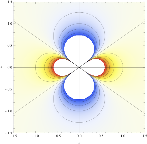
Figure 1: The contour plot of the induced charge density (35) in the plane $x_{1}=x\,,x_{3}=z$. The 3-D pattern is to be obtained by a half-revolution around the axiz $x_{2}=y$. In the polar cones $|z|>|x/\sqrt{2}|$ $\left(|\zeta|<\arccos\left(1/\sqrt{3}\right)\right)$ – (blue online) – the charge density is negative, while it is positive in the equatorial zone – (yellow - red online). The solid lines are those of a constant charge density, the latter being zero on the separating straight lines $z=x/\sqrt{2}$. Owing to the $1/r^{3}$ dependence, regions close to the origin could not be handled by the code and are left blank.

3.2.2 Nonlinearly modified Coulomb field

The electric correction (27) is calculated in Appendix B. It can be split into two parts:

$$\mathbf{E}^{\left(1\right)}\left(\mathbf{x}\right)=\mathbf{E}_{\mathrm{in}}^{\left(1\right)}\left(\mathbf{x}\right)\theta\left(R-r\right)+\mathbf{E}_{\mathrm{out}}^{\left(1\right)}\left(\mathbf{x}\right)\theta\left(r-R\right)\,,$$ (36)

where the inner $\mathbf{E}_{\mathrm{in}}^{\left(1\right)}\left(\mathbf{x}\right)$ component corresponds to points inside the Coulomb source,

$$\mathbf{E}_{\mathrm{in}}^{\left(1\right)}\left(\mathbf{x}\right) = \frac{q}{4\pi}\frac{1}{R^{3}}\left(\mathfrak{L}_{\mathfrak{F}}+\frac{\tilde{b}}{5}\right)\mathbf{x}-\frac{2}{5R^{3}}\left(\frac{q}{4\pi}\right)\left[\mathfrak{L}_{\mathfrak{FF}}\left(\mathbf{\overline{E}}\cdot\mathbf{x}\right)+\mathfrak{L}_{\mathfrak{FG}}\left(\mathbf{\overline{B}}\cdot\mathbf{x}\right)\right]\mathbf{\overline{E}}$$ (37)

$$- \frac{2}{5R^{3}}\left(\frac{q}{4\pi}\right)\left[\mathfrak{L}_{\mathfrak{FG}}\left(\mathbf{\overline{E}}\cdot\mathbf{x}\right)+\mathfrak{L}_{\mathfrak{GG}}\left(\mathbf{\overline{B}}\cdot\mathbf{x}\right)\right]\mathbf{\overline{B}\,,}$$

while $\mathbf{E}_{\mathrm{out}}^{\left(1\right)}\left(\mathbf{x}\right)$ corresponds to the electric field at points outside the Coulomb source

$$\mathbf{E}_{\mathrm{out}}^{\left(1\right)}\left(\mathbf{x}\right) = \frac{q}{4\pi}\left\{\mathfrak{L}_{\mathfrak{F}}+\left(1-\frac{3R^{2}}{5r^{2}}\right)\frac{\tilde{b}}{2}+\frac{3}{2r^{2}}\left(1-\frac{R^{2}}{r^{2}}\right)\times\right.$$ (38)

$$\times \left.\left[\mathfrak{L}_{\mathfrak{FF}}\left(\mathbf{\overline{E}}\cdot\mathbf{x}\right)^{2}+\mathfrak{L}_{\mathfrak{GG}}\left(\mathbf{\overline{B}}\cdot\mathbf{x}\right)^{2}+2\mathfrak{L}_{\mathfrak{FG}}\left(\mathbf{\overline{B}}\cdot\mathbf{x}\right)\left(\mathbf{\overline{E}}\cdot\mathbf{x}\right)\right]\right\}\frac{\mathbf{x}}{r^{3}}$$

$$- \frac{q}{4\pi}\frac{1}{r^{3}}\left(1-\frac{3R^{2}}{5r^{2}}\right)\left[\mathfrak{L}_{\mathfrak{FF}}\left(\mathbf{\overline{E}}\cdot\mathbf{x}\right)+\mathfrak{L}_{\mathfrak{FG}}\left(\mathbf{\overline{B}}\cdot\mathbf{x}\right)\right]\mathbf{\overline{E}}$$

$$- \frac{q}{4\pi}\frac{1}{r^{3}}\left(1-\frac{3R^{2}}{5r^{2}}\right)\left[\mathfrak{L}_{\mathfrak{FG}}\left(\mathbf{\overline{E}}\cdot\mathbf{x}\right)+\mathfrak{L}_{\mathfrak{GG}}\left(\mathbf{\overline{B}}\cdot\mathbf{x}\right)\right]\mathbf{\overline{B}}\,.$$

The electric field given by Eqs. (36), (37), (38) is continuous on the surface of the sphere $r=R$, the boundary of the charge (13). Note that the $R$-dependent, fast decreasing at $\left(r/R\right)\rightarrow\infty,$ part

$$\mathbf{E}_{\mathrm{out}}^{\left(1\right)}\left(\mathbf{x};R\right) = \frac{q}{4\pi}\left\{\left(-\frac{3R^{2}}{5r^{2}}\right)\frac{\tilde{b}}{2}-\frac{3}{2r^{2}}\left(\frac{R^{2}}{r^{2}}\right)\times\right.$$

$$\times \left.\left[\mathfrak{L}_{\mathfrak{FF}}\left(\mathbf{\overline{E}}\cdot\mathbf{x}\right)^{2}+\mathfrak{L}_{\mathfrak{GG}}\left(\mathbf{\overline{B}}\cdot\mathbf{x}\right)^{2}+2\mathfrak{L}_{\mathfrak{FG}}\left(\mathbf{\overline{B}}\cdot\mathbf{x}\right)\left(\mathbf{\overline{E}}\cdot\mathbf{x}\right)\right]\right\}\frac{\mathbf{x}}{r^{3}}$$

$$+ \frac{q}{4\pi}\frac{1}{r^{3}}\left(\frac{3R^{2}}{5r^{2}}\right)\left[\mathfrak{L}_{\mathfrak{FF}}\left(\mathbf{\overline{E}}\cdot\mathbf{x}\right)+\mathfrak{L}_{\mathfrak{FG}}\left(\mathbf{\overline{B}}\cdot\mathbf{x}\right)\right]\mathbf{\overline{E}}$$

$$+ \frac{q}{4\pi}\frac{1}{r^{3}}\left(\frac{3R^{2}}{5r^{2}}\right)\left[\mathfrak{L}_{\mathfrak{FG}}\left(\mathbf{\overline{E}}\cdot\mathbf{x}\right)+\mathfrak{L}_{\mathfrak{GG}}\left(\mathbf{\overline{B}}\cdot\mathbf{x}\right)\right]\mathbf{\overline{B}}\,,$$

of the outer field (38) is a solution of the sourceless equation $\mathbf{\nabla\cdot E}_{\mathrm{out}}^{\left(1\right)}\left(\mathbf{x};R\right)=0$. This is not unexpected, because the source (30) does not contain $R$. The hidden role of adding the free solution $\mathbf{E}_{\mathrm{out}}^{\left(1\right)}\left(\mathbf{x};R\right)$ is only to provide the continuity. It has appeared automatically within the calculation of the projection (27).

3.2.3 Parallel background fields

For a simplifying special case of external fields parallel $\mathbf{\overline{E}\parallel\overline{B}}$ in the rest frame of the charge (or antiparallel in the spatially reflected frame), $\mathbf{\overline{B}}=\overline{B}\boldsymbol{\mu}$, $\mu=1$ the results (37) and (38) above take the cylindric-symmetrical form $\mathbf{E}^{(1)}=\alpha(r,\zeta)\mathbf{x}+\beta(r,\zeta)\boldsymbol{\mu}$, namely

$$\mathbf{E}_{\mathrm{in}}^{\left(1\right)}\left(\mathbf{x}\right)=\frac{q}{4\pi}\left[\frac{1}{5R^{3}}\left(5\mathfrak{L}_{\mathfrak{F}}+\tilde{b}\right)\mathbf{x}+\frac{2\tilde{b}r}{5R^{3}}\left(\frac{\boldsymbol{\mu}\cdot\mathbf{x}}{r}\right)\boldsymbol{\mu}\right]\,,$$ (39)

and

$$\mathbf{E}_{\mathrm{out}}^{\left(1\right)}\left(\mathbf{x}\right) = \frac{q}{4\pi}\left[\mathfrak{L}_{\mathfrak{F}}+\frac{\tilde{b}}{2}\left(1-\frac{3R^{2}}{5r^{2}}\right)-\frac{3\tilde{b}}{2}\left(1-\frac{R^{2}}{r^{2}}\right)\left(\frac{\boldsymbol{\mu}\cdot\mathbf{x}}{r}\right)^{2}\right]\frac{\mathbf{x}}{r^{3}}$$ (40)

$$+ \frac{q}{4\pi}\frac{\tilde{b}}{r^{2}}\left(1-\frac{3R^{2}}{5r^{2}}\right)\left(\frac{\boldsymbol{\mu}\cdot\mathbf{x}}{r}\right)\boldsymbol{\mu}\,.$$

The structural functions $\alpha(r,\zeta)$ and $\beta(r,\zeta)\boldsymbol{\ }$are, respectively, even and odd in the angular variable $\zeta=\left(\mathbf{x}\cdot\boldsymbol{\mu}\right)/r$ because $\boldsymbol{\mu}$ is a pseudovector, while $q\tilde{b}$ and $q\mathfrak{L}_{\mathfrak{F}}$ are scalars. In the limit $R/r\rightarrow 0$, the free part

$$\frac{3\tilde{b}q}{8\pi}R^{2}\left\{\left[-\frac{1}{5}+\left(\frac{\boldsymbol{\mu}\cdot\mathbf{x}}{r}\right)^{2}\right]\frac{\mathbf{x}}{r^{5}}-\frac{2}{5}\left(\frac{\boldsymbol{\mu}\cdot\mathbf{x}}{r}\right)\frac{\boldsymbol{\mu}}{r^{4}}\right\}\,,$$ (41)

of the outer field disappears, such that (40) becomes the electric field generated by a pointlike particle $\mathbf{E}_{\mathrm{PL}}^{\left(1\right)}\left(\mathbf{x}\right)$, valid for every $r>0$

$$\lim_{R\rightarrow 0}\mathbf{E}_{\mathrm{out}}^{\left(1\right)}\left(\mathbf{x}\right)=\mathbf{E}_{\mathrm{PL}}^{\left(1\right)}\left(\mathbf{x}\right)=\frac{q}{4\pi}\left[\mathfrak{L}_{\mathfrak{F}}+\frac{\tilde{b}}{2}\left(1-3\zeta^{2}\right)\right]\frac{\mathbf{x}}{r^{3}}+\frac{q}{4\pi}\frac{\tilde{b}}{r^{2}}\zeta\boldsymbol{\mu}\,,\ \ r>0\,,$$ (42)

with $\zeta=\frac{\boldsymbol{\mu}\cdot\mathbf{x}}{r}$ being the azimuth angle cosine. The induced charge density corresponding to such a limit $\rho_{\mathrm{PL}}^{\left(1\right)}=\boldsymbol{\nabla}\cdot\mathbf{E}_{\mathrm{PL}}^{\left(1\right)}\left(\mathbf{x}\right)$ distributed outside the origin is

$$\rho_{\mathrm{PL}}^{\left(1\right)}=\frac{q\tilde{b}}{4\pi r^{3}}\left(1-3\zeta^{2}\right)\,,\text{ }r>0\,.$$

Therefore, the total charge concentrated in the volume $V$ between any two spheres of finite radii $r_{1}$ and $r_{2}$ is zero:

$$\int_{V}\rho_{\mathrm{PL}}^{\left(1\right)}d^{3}x=\frac{q\tilde{b}}{2}\int_{r_{1}}^{r_{2}}\frac{dr}{r}\int_{-1}^{1}\left(1-3\zeta^{2}\right)d\zeta=0\,,$$

in agreement with the general case of nonparallel background fields (31). On the other hand, the flux of the field (42) through the surface of a sphere centered in the origin is different from zero (and independent of the radius)

$$\oint_{S}\mathbf{E}_{\mathrm{PL}}^{\left(1\right)}\left(\mathbf{x}\right)\cdot\mathbf{\hat{n}}dS=q\left(\mathfrak{L}_{\mathfrak{F}}+\frac{1}{3}\tilde{b}\right)\,,$$ (43)

which coincides with (32). Because of the Gauss theorem $\oint_{S}\mathbf{E}^{\left(1\right)}\left(\mathbf{x}\right)\cdot\mathbf{\hat{n}}dS=\int_{V}d^{3}x\mathbf{\nabla\cdot E}^{\left(1\right)}\left(\mathbf{x}\right)$ this implies that the distribution of the induced charge $\rho^{(1)}=\mathbf{\nabla\cdot E}^{\left(1\right)}\left(\mathbf{x}\right)$ in parallel constant background fields is

$$\rho_{\mathrm{point}}^{(1)}=\frac{q}{4\pi}\left[\left(\mathfrak{L}_{\mathfrak{F}}+\frac{\tilde{b}}{3}\right)\delta^{3}\left(\mathbf{x}\right)+\frac{\tilde{b}}{r^{3}}\left(1-3\left(\frac{\boldsymbol{\mu}\cdot\mathbf{x}}{r}\right)^{2}\right)\right]\,,$$

following the definition of the Dirac delta-function in terms of an integral. Note that formally the second term here, as well as in (34), has a $r^{-3}$ singularity in the origin. Certainly this singularity should not be taken seriously, because the whole infrared approximation on which our present approach is based fails in this point. Nevertheless this singularity itself is not significant, since the overall distributed charge is zero thanks to the angle integration.

3.2.4 Scalar potential

As long as the fulfillment of identities (6) is provided, the result for the modified Coulomb field must have a potential representation $\mathbf{E}^{\left(1\right)}\left(\mathbf{x}\right)=-\boldsymbol{\nabla}A_{0}^{(1)}\left(\mathbf{x}\right)$. For the cylindrically symmetric case of parallel background fields the field (39) and (40) corresponds to the potential

$$A_{0}^{(1)}\left(\mathbf{x}\right)=A_{0}^{(1)\mathrm{in}}\left(\mathbf{x}\right)\theta\left(R-r\right)+A_{0}^{(1)\mathrm{out}}\left(\mathbf{x}\right)\theta\left(r-R\right)\,,$$

where its inner and outer parts are of the form

$$A_{0}^{(1)\mathrm{in}}\left(\mathbf{x}\right)=\mathrm{const.}+r^{2}\lambda_{1}\left(\zeta^{2}\right)\,,\text{ \ }A_{0}^{(1)\mathrm{out}}\left(\mathbf{x}\right)=\frac{\lambda_{2}\left(\zeta^{2}\right)}{r}+\frac{\lambda_{3}\left(\zeta^{2}\right)}{r^{3}}\,,$$

namely

$$A_{0}^{(1)\mathrm{in}}\left(\mathbf{x}\right) = \frac{q}{4\pi}\left\{\frac{1}{2R}\left(3\mathfrak{L}_{\mathfrak{F}}+\tilde{b}\right)-\frac{1}{5R^{3}}\left[\frac{1}{2}\left(\tilde{b}+5\mathfrak{L}_{\mathfrak{F}}\right)+\tilde{b}\zeta^{2}\right]r^{2}\right\}\,,$$

$$A_{0}^{(1)\mathrm{out}}\left(\mathbf{x}\right) = \frac{q}{4\pi}\left\{\frac{1}{r}\left[\mathfrak{L}_{\mathfrak{F}}+\frac{\tilde{b}}{2}\left(1-\zeta^{2}\right)\right]+\frac{\tilde{b}R^{2}}{10r^{3}}\left(3\zeta^{2}-1\right)\right\}\,.$$ (44)

The structural coefficient functions $\lambda_{1,2,3}\left(\zeta^{2}\right)$ are even in $\zeta=\frac{\mathbf{x\cdot}\overline{\mathbf{B}}}{r\overline{B}}$ because the latter is a pseudoscalar, while $\tilde{b}$ and $\mathfrak{L}_{\mathfrak{F}}$ are scalars. The written potential is continuous at $r=R$ everywhere at the sphere surface. Its part $\frac{q}{4\pi}\frac{\tilde{b}R^{2}}{10r^{3}}\left(3\zeta^{2}-1\right)$ depending on $R$ satisfies the free equation $\boldsymbol{\nabla}^{2}A_{0}^{(1)\mathrm{out}}=0$ out of the core, as it should. This is the quadrupole addition to the potential in the case of cylindric symmetry [31], the quadrupole moment being $\frac{q}{4\pi}\frac{\tilde{b}R^{2}}{5}$. It disappears together with $R$, which means that for the pointlike initial charge the induced charge contribution does not possess a quadrupole moment. The boundary conditions for the scalar potential have been chosen so as to provide finiteness at $r=0$ and decreasing at $r\rightarrow\infty$.

We present in Fig. 2 the pattern of electric lines of force following Eq. (42) and the equipotential lines, corresponding to the pointlike limit of Eq. (44) at $r>0$

$$A_{0}^{(1)\mathrm{PL}}\left(\mathbf{x}\right)=\frac{q}{4\pi}\frac{1}{r}\left[\mathfrak{L}_{\mathfrak{F}}+\frac{\tilde{b}}{2}\left(1-\zeta^{2}\right)\right]\,,$$ (45)

which is also the asymptotic behavior of the potential Eq. (44) in the far-off domain.

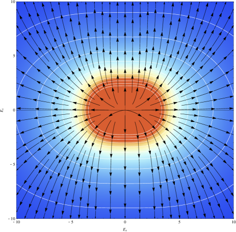
Figure 2: Electric lines of force (42) (represented by black arrows) and the corresponding equipotential curves (45) (represented by white lines) of a point-like source placed in external constant electric and magnetic fields directed along the $z$ axis. We set $q>0$ and $\left(q/4\pi\right)\mathfrak{L}_{\mathfrak{F}}=1=\left(q/4\pi\right)\tilde{b}$. The electric field is more intense close to the origin, represented by the red region, becoming weaker far from the origin, represented by the blue regions. The complete pattern corresponds to the modification of the standard Coulombic electric lines of force and its equipotential lines.

It remains to confront the present results with those obtained previously for purely magnetic background [19] [20]. For that case, using a different method, the following expression for the scalar potential of a point charge in a magnetic field $\overline{\mathbf{B}}$ in the far-off region (the anisotropic Coulomb law) was finally presented as Eq. (27) in Ref. [7]:

$$A_{0}(\mathbf{x})=\frac{q}{4\pi}\frac{1}{\sqrt{\varepsilon_{\perp}}\sqrt{\varepsilon_{\perp}x_{{}_{\parallel}}^{2}+\varepsilon_{{}_{\parallel}}\mathbf{x}_{\perp}^{2}}},$$ (46)

where $\varepsilon_{\perp}=1-\mathfrak{L}_{\mathfrak{F}}$ and  $\varepsilon_{{}_{\parallel}}=1-\mathfrak{L}_{\mathfrak{F}}+2\overline{\mathfrak{F}}\mathfrak{L}_{\mathfrak{G}\mathfrak{G}}\$are eigenvalues of the dielectric tensor [32] $\varepsilon_{ij}=\left(1-\mathfrak{L}_{\mathfrak{F}}\right)\delta_{ij}+\mathfrak{L}_{\mathfrak{G}\mathfrak{G}}\overline{B}_{i}\overline{B}_{j},$ responsible for polarization induced by homogeneously charged planes parallel and orthogonal to $\overline{\mathbf{B}}$, respectively, [33]. In Eq. (46), $\mathbf{x}_{\perp}=r\sin\theta$ and $\mathbf{x}_{\parallel}=r\cos\theta$ are the coordinate components across and along $\overline{\mathbf{B}}$, respectively. Taking this into account we rewrite the anisotropic Coulomb potential (46) as

$$A_{0}(\mathbf{x})=\frac{q}{4\pi r}\frac{1}{\sqrt{\varepsilon_{\perp}}\sqrt{\varepsilon_{\perp}\cos^{2}\theta+\varepsilon_{{}_{\parallel}}\sin^{2}\theta}}=\frac{q}{4\pi r}\frac{1}{\sqrt{\varepsilon_{\perp}}\sqrt{1-\mathfrak{L}_{\mathfrak{F}}+2\overline{\mathfrak{F}}\mathfrak{L}_{\mathfrak{G}\mathfrak{G}}\sin^{2}\theta}}.$$ (47)

Considering the corrections $\mathfrak{L}_{\mathfrak{F}}$ and $2\overline{\mathfrak{F}}\mathfrak{L}_{\mathfrak{G}\mathfrak{G}}$ to the vacuum dielectric permeability $\epsilon=1$ as small, we find that in this approximation Eq. (47) turns into $\frac{q}{4\pi r}\left[1+\mathfrak{L}_{\mathfrak{F}}-\mathfrak{L}_{\mathfrak{GG}}\overline{\mathfrak{F}}\left(1-\zeta^{2}\right)\right],$ which is just $\frac{q}{4\pi r}+A_{0}^{(1)\mathrm{PL}}\left(\mathbf{x}\right),$ Eq. (45), with $\tilde{b}=-2\mathfrak{L}_{\mathfrak{GG}}\overline{\mathfrak{F}}$ obtained by setting $\mathbf{\overline{E}}^{2}=\overline{\mathfrak{G}}=0$ in (33). The important difference between the results (46) or (47), on one hand, and (45), on the other, is that the former were obtained using the full photon propagator component $D_{00}=$ ($\boldsymbol{k}^{2}-\varkappa_{2})^{-1}$ (in the momentum representation) with $\varkappa_{2}=\boldsymbol{k}^{2}\mathfrak{L}_{\mathfrak{F}}-k_{\parallel}^{2}2\overline{\mathfrak{F}}\mathfrak{L_{GG}}$. Here $\boldsymbol{k}^{2}=\boldsymbol{k}_{\perp}^{2}+k_{\parallel}^{2},$ and $\boldsymbol{k}_{\perp}$ and $k_{\parallel}$ are the momentum components across and along $\overline{\boldsymbol{B}}$ , respectively. The full propagator is decomposed into the series

$$D_{00}=\frac{1}{\boldsymbol{k}^{2}-\varkappa_{2}}=\frac{1}{\boldsymbol{k}^{2}}+\frac{1}{\boldsymbol{k}^{2}}\frac{\varkappa_{2}}{\boldsymbol{k}^{2}}+...,$$ (48)

corresponding to the summation of the one-photon-reducible chain of one- electron-positron loop diagrams. On the contrary, the correction (45) corresponds to the second term in this expansion alone, since only the free photon propagator $\frac{1}{\boldsymbol{\nabla}^{2}}=\frac{1}{\boldsymbol{k}^{2}}$ was used in (25) for finding the field of a point charge. As a consequence, there is a difference in the convexity of the lines of force in Fig. 2 as compared to Fig. 2b in Ref. [21] and, correspondingly, in the orientation of the equipotential ellipsoid as compared to Fig. 1 in Ref. [23]. The summation of the chain, though not strictly grounded, was crucial for establishing [19] the squeezing of the Coulomb field into a string in the limit of infinite magnetic field and for the screening of the Coulomb field by a strong magnetic field that prevents the collapse of the hydrogen atom in the limit $\overline{B}\rightarrow\infty$ (see also [20, 23]).

4 Considerations within the Euler-Heisenberg effective Lagrangian

It is most interesting to apply the formulas of the previous sections valid for the arbitrary local nonlinear theory to quantum electrodynamics approximated by the Euler-Heisenberg (EH) effective Lagrangian [8]. This is what we shall be doing in the present Section where, for the sake of simplicity, we omit bars over the background fields.

According to Refs. [8, 10] it is written as

$$\mathfrak{L}=\frac{m^{4}}{8\pi^{2}}\int_{0}^{\infty}dt\frac{e^{-t}}{t^{3}}\left\{-\left(ta\cot ta\right)\left(tb\coth tb\right)+1-\frac{1}{3}\left(a^{2}-b^{2}\right)t^{2}\right\}\,,$$ (49)

where the integration contour is meant to circumvent the poles on the real axis of $t$ supplied by $\cot ta$ above the real axis. Because of the exponentially fast decrease of the integrand at $t\rightarrow\infty$ we may equivalently accept that the integration path is a straight ray inclined by an infinitesimally small angle to the real axis in the upper complex plane. This circumstance will be significant in the situation treated in Sec. 4.2.2 where the Schwinger effect of pair creation from the vacuum might come into play.

In (49), the dimensionless invariant combinations, eigenvalues of the field tensor,

$$a=\left(\frac{e}{m^{2}}\right)\sqrt{-\mathfrak{F}+\sqrt{\mathfrak{F}^{2}+\mathfrak{G}^{2}}}\,,$$

$$b=\left(\frac{e}{m^{2}}\right)\sqrt{\mathfrak{F}+\sqrt{\mathfrak{F}^{2}+\mathfrak{G}^{2}}}\,$$ (50)

have the meaning of the electric and magnetic field in a Lorentz frame in which these are parallel, normalized to the characteristic field value $\frac{e}{m^{2}}$, where $m$ and $e$ are the electron mass and charge, respectively. Such a frame exists as long as $\mathfrak{G}\neq 0.$ Since in the previous sections we mostly dealt with the general case where the fields are not necessarily parallel in the rest frame of the charge, we shall not generally identify $a$ with $eE/m^{2}$ and $b$ with $eB/m^{2}$.

4.1 Small background fields

In the small-field limit, $a,b\ll 1,$ we should take the (lowest) quadratic approximation for the Euler-Heisenberg Lagrangian (49) known to be

$$\mathfrak{L}_{\mathrm{weak}}\simeq\frac{1}{8\pi^{2}}\left(\frac{e^{4}}{m^{4}}\right)\left(\frac{4\mathfrak{F}^{2}+7\mathfrak{G}^{2}}{45}\right)\,.$$

Hence, the coefficients involved in our previous formulas should be defined in this approximation by Eqs. (8) with $\mathcal{F}=0$. One has $\mathfrak{L}_{\mathfrak{FF}}=\frac{1}{8\pi^{2}}\left(\frac{e^{4}}{m^{4}}\right)\left(\frac{8}{45}\right),$ $\mathfrak{L}_{\mathfrak{GG}}=\frac{1}{8\pi^{2}}\left(\frac{e^{4}}{m^{4}}\right)\left(\frac{14}{45}\right),$ $\mathfrak{L}_{\mathfrak{FG}}=0$, and $\mathfrak{L}_{\mathfrak{F}}=0$. With this substitution, the induced charge Eq. (32), for instance becomes

$$Q_{\mathrm{in}}=-\frac{q}{12\pi^{2}}\left(\frac{e^{4}}{45m^{4}}\right)\left(4\mathbf{E}^{2}+7\mathbf{B}^{2}\right)\,.$$

4.2 Strong background fields

In the general case of arbitrarily strong fields the necessary coefficients are calculated from (62). With the help of (50) and two auxiliary functions $\mathcal{H}\left(\tau\right)$ and $\mathcal{Q}\left(\tau\right)$,

$$\mathcal{H}\left(\tau\right)=\tau\coth\tau-\frac{\tau^{2}}{\sinh^{2}\tau}\,,\ \ \mathcal{Q}\left(\tau\right)=\tau\cot\tau-\frac{\tau^{2}}{\sin^{2}\tau}\,,$$ (51)

the derivative of (49) with respect to $\mathfrak{F}$ can be expressed as

$$\mathfrak{L}_{\mathfrak{F}} = \frac{m^{4}}{16\pi^{2}}\frac{b^{2}}{\sqrt{\mathfrak{F}^{2}+\mathfrak{G}^{2}}}\int_{0}^{\infty}d\tau\frac{e^{-\tau/b}}{\tau^{3}}\left\{-\mathcal{H}\left(\tau\right)\left(\frac{a\tau}{b}\cot\frac{a\tau}{b}\right)\right.$$ (52)

$$+ \left.\left(\tau\coth\tau\right)\mathcal{Q}\left(\frac{a\tau}{b}\right)+\frac{2\tau^{2}}{3}\left[1+\left(\frac{a}{b}\right)^{2}\right]\right\}\,.$$

Introducing two more constants $\gamma_{\pm}$ and new auxiliary functions $\mathcal{\tilde{H}}\left(\tau\right)$ and $\mathcal{\tilde{Q}}\left(\tau\right)$,

$$\gamma_{\pm}=1\pm\frac{2\mathfrak{F}}{\sqrt{\mathfrak{F}^{2}+\mathfrak{G}^{2}}}\,,$$

$$\mathcal{\tilde{Q}}\left(\tau\right)=\frac{2\tau^{2}}{\sin^{2}\tau}\left(\tau\cot\tau-1\right)\,,\ \ \mathcal{\tilde{H}}\left(\tau\right)=\frac{2\tau^{2}}{\sinh^{2}\tau}\left(\tau\coth\tau-1\right)\,.$$ (53)

the second-order derivatives involved in the definition of $\tilde{b}$ (33) are:

$$\mathfrak{L}_{\mathfrak{FF}} = \frac{m^{4}}{32\pi^{2}}\frac{b^{2}}{\left(\mathfrak{F}^{2}+\mathfrak{G}^{2}\right)}\int_{0}^{\infty}d\tau\frac{e^{-\tau/b}}{\tau^{3}}\left\{2\mathcal{H}\left(\tau\right)\mathcal{Q}\left(\frac{a\tau}{b}\right)\right.$$

$$- \tau\coth\tau\left[\gamma_{+}\mathcal{Q}\left(\frac{a\tau}{b}\right)+\mathcal{\tilde{Q}}\left(\frac{a\tau}{b}\right)\right]$$

$$- \left.\left(\frac{a\tau}{b}\cot\frac{a\tau}{b}\right)\left[\gamma_{-}\mathcal{H}\left(\tau\right)+\mathcal{\tilde{H}}\left(\tau\right)\right]\right\}\,,$$

$$\mathfrak{L}_{\mathfrak{GG}} = \frac{m^{4}}{32\pi^{2}}\frac{b^{2}}{\left(\mathfrak{F}^{2}+\mathfrak{G}^{2}\right)}\int_{0}^{\infty}d\tau\frac{e^{-\tau/b}}{\tau^{3}}\left\{-2\mathcal{H}\left(\tau\right)\mathcal{Q}\left(\frac{a\tau}{b}\right)\right.$$

$$- \tau\coth\tau\left[-\gamma_{+}\mathcal{Q}\left(\frac{a\tau}{b}\right)+\frac{b^{2}}{a^{2}}\mathcal{\tilde{Q}}\left(\frac{a\tau}{b}\right)\right]$$

$$- \left.\left(\frac{a\tau}{b}\cot\frac{a\tau}{b}\right)\left[-\gamma_{-}\mathcal{H}\left(\tau\right)+\frac{a^{2}}{b^{2}}\mathcal{\tilde{H}}\left(\tau\right)\right]\right\}\,,$$

$$\mathfrak{L}_{\mathfrak{FG}} = \frac{m^{4}\kappa}{32\pi^{2}}\frac{b^{2}}{\left(\mathfrak{F}^{2}+\mathfrak{G}^{2}\right)}\int_{0}^{\infty}d\tau\frac{e^{-\tau/b}}{\tau^{3}}\left\{\frac{1}{ab}\left(a^{2}-b^{2}\right)\mathcal{H}\left(\tau\right)\mathcal{Q}\left(\frac{a\tau}{b}\right)\right.$$ (54)

$$+ \frac{b\tau}{a}\coth\tau\left[-\gamma_{-}\mathcal{Q}\left(\frac{a\tau}{b}\right)+\mathcal{\tilde{Q}}\left(\frac{a\tau}{b}\right)\right]$$

$$+ \left.\frac{a}{b}\left(\frac{a\tau}{b}\cot\frac{a\tau}{b}\right)\left[\gamma_{+}\mathcal{H}\left(\tau\right)-\mathcal{\tilde{H}}\left(\tau\right)\right]\right\}\,.$$

It should be noted that $\mathfrak{L}_{\mathfrak{FG}}$ as a pseudoscalar is an odd function, as expressed by the constant $\kappa=\mathrm{sign}\left(\mathfrak{G}\right)$.

4.2.1 Magnetic-dominated large-field regime

We can represent Eqs. (52), (54) as functions of $b$ and of the ratio $a/b$, that can be then expanded in powers of the latter assuming that

$$\frac{a}{b}\ll 1,$$ (55)

but irrespective of whether $a\$ and $b$ are small or not as compared to unity. Condition (55) implies the magnetic dominance $B\gg E$ in any reference frame. The expansion of (52) and (54) includes the expansion of the trigonometric cotangent in the power series of its argument. Thereby the poles at the real axis are avoided in accord with the well-known fact that an expansion over the (relatively) small electric field excludes the Schwinger effect. Then by virtue of (55), every coefficient is expressed as a power series of the ratio $a/b$,

$$\mathfrak{L}_{k}=\mathfrak{L}_{k}^{\left(0\right)}+\left(\frac{a}{b}\right)^{2}\mathfrak{L}_{k}^{\left(2\right)}+O\left[\left(\frac{a}{b}\right)^{4}\right]\,,$$ (56)

where $k$ simply labels distinct coefficients, i. e., $k=\left\{\mathfrak{F},\mathfrak{FF},\mathfrak{GG},\mathfrak{FG}\right\}$. It should be noted that the identity $\mathfrak{L}_{\mathfrak{FG}}^{\left(0\right)}=0$ is a consequence of the fact that $\mathfrak{L}_{\mathfrak{FG}}$ must be absent when the electric field is zero. We obtain, for the leading $\mathfrak{L}_{k}^{\left(0\right)}$ and the next-to-leading $\mathfrak{L}_{k}^{\left(2\right)}$ terms, the following expressions

$$\mathfrak{L}_{\mathfrak{F}}^{\left(0\right)} = \frac{\alpha}{2\pi}\int_{0}^{\infty}d\tau\frac{e^{-\tau/b}}{\tau}\left(\frac{2}{3}-\frac{\coth\tau}{\tau}+\frac{1}{\sinh^{2}\tau}\right)\,,$$

$$\mathfrak{L}_{\mathfrak{F}}^{\left(2\right)} = \frac{\alpha}{2\pi}\int_{0}^{\infty}d\tau\frac{e^{-\tau/b}}{\tau}\left[\left(\frac{1}{\tau}-\frac{\tau}{3}\right)\coth\tau-\left(1+\frac{\tau^{2}}{3}\right)\frac{1}{\sinh^{2}\tau}\right]\,,$$ (57)

for the first derivatives and

$$\left(\mathfrak{F}+\sqrt{\mathfrak{F}^{2}+\mathfrak{G}^{2}}\right)\mathfrak{L}_{\mathfrak{FF}}^{\left(0\right)} = \frac{\alpha}{2\pi}\int_{0}^{\infty}d\tau\frac{e^{-\tau/b}}{\tau}\left(\frac{1}{\tau}\coth\tau+\frac{1}{\sinh^{2}\tau}-\frac{2\tau\coth\tau}{\sinh^{2}\tau}\right)\,,$$

$$\left(\mathfrak{F}+\sqrt{\mathfrak{F}^{2}+\mathfrak{G}^{2}}\right)\mathfrak{L}_{\mathfrak{FF}}^{\left(2\right)} = \frac{\alpha}{2\pi}\int_{0}^{\infty}d\tau\frac{e^{-\tau/b}}{\tau}\left[\left(\tau-\frac{6}{\tau}\right)\coth\tau+\frac{\left(2+\tau^{2}\right)}{\sinh^{2}\tau}\right.$$

$$+ \left.\left(\frac{2\tau^{2}}{3}+4\right)\frac{\tau\coth\tau}{\sinh^{2}\tau}\right]\,,$$

$$\left(\mathfrak{F}+\sqrt{\mathfrak{F}^{2}+\mathfrak{G}^{2}}\right)\mathfrak{L}_{\mathfrak{GG}}^{\left(0\right)} = \frac{\alpha}{2\pi}\int_{0}^{\infty}d\tau\frac{e^{-\tau/b}}{\tau}\left(\frac{2\tau}{3}\coth\tau-\frac{1}{\tau}\coth\tau+\frac{1}{\sinh^{2}\tau}\right)\,,$$

$$\left(\mathfrak{F}+\sqrt{\mathfrak{F}^{2}+\mathfrak{G}^{2}}\right)\mathfrak{L}_{\mathfrak{GG}}^{\left(2\right)} = \frac{\alpha}{2\pi}\int_{0}^{\infty}d\tau\frac{e^{-\tau/b}}{\tau}\left[\left(\frac{4\tau^{3}}{15}+\frac{6}{\tau}-\frac{5\tau}{3}\right)\coth\tau\right.$$

$$- \left.\left(4+\frac{5\tau^{2}}{3}\right)\frac{1}{\sinh^{2}\tau}-\frac{2\tau\coth\tau}{\sinh^{2}\tau}\right]\,,$$

$$\left(\mathfrak{GL}_{\mathfrak{FG}}\right)^{\left(2\right)} = \frac{\alpha}{2\pi}\int_{0}^{\infty}d\tau\frac{e^{-\tau/b}}{\tau}\left[\left(\frac{3}{\tau}-\frac{2\tau}{3}\right)\coth\tau\right.$$ (58)

$$- \left.\left(1+\frac{2\tau^{2}}{3}\right)\frac{1}{\sinh^{2}\tau}-\frac{2\tau\coth\tau}{\sinh^{2}\tau}\right]\,,$$

for the second derivatives.

This representation allows us to consider the asymptotic regime of large magnetic field with the electric field kept moderate by studying the $b\gg 1$ limit. In this regime the coefficient $\mathfrak{L}_{\mathfrak{GG}}$ dominates over every other coefficient in our expressions for the fields and charges, since the integrals (57) and (58) over $\tau$ would diverge linearly for $\left(\mathfrak{F}+\sqrt{\mathfrak{F}^{2}+\mathfrak{G}^{2}}\right)\mathfrak{L}_{\mathfrak{GG}}^{\left(0\right)}$ and cubically for $\left(\mathfrak{F}+\sqrt{\mathfrak{F}^{2}+\mathfrak{G}^{2}}\right)\mathfrak{L}_{\mathfrak{GG}}^{\left(2\right)}$ if the limit $b=\infty$ had been formally substituted into their integrands. To be more rigorous, the asymptotic forms of Eqs. (57) and (58) read

$$\mathfrak{L}_{\mathfrak{F}}^{\left(0\right)}\simeq\frac{\alpha}{2\pi}\left(\frac{2}{3}\log b+\mathcal{K}_{\mathfrak{F}}^{\left(0\right)}\right)\,,\ \ \mathfrak{L}_{\mathfrak{F}}^{\left(2\right)}\simeq\frac{\alpha}{2\pi}\left(-\frac{b}{3}+\mathcal{K}_{\mathfrak{F}}^{\left(2\right)}\right)\,,\ \ \left(\mathcal{K}_{\mathfrak{F}}^{\left(0\right)},\mathcal{K}_{\mathfrak{F}}^{\left(2\right)}\right)=\mathrm{const.}\,,$$ (59)

and

$$\left(\mathfrak{F}+\sqrt{\mathfrak{F}^{2}+\mathfrak{G}^{2}}\right)\mathfrak{L}_{\mathfrak{FF}}^{\left(0\right)}\simeq\frac{\alpha}{2\pi}\mathcal{K}_{\mathfrak{FF}}^{\left(0\right)}\,,\ \ \mathcal{K}_{\mathfrak{FF}}^{\left(0\right)}=\mathrm{const.\,,}$$

$$\left(\mathfrak{F}+\sqrt{\mathfrak{F}^{2}+\mathfrak{G}^{2}}\right)\mathfrak{L}_{\mathfrak{FF}}^{\left(2\right)}\simeq\frac{\alpha}{2\pi}\left(b+\mathcal{K}_{\mathfrak{FF}}^{\left(2\right)}\right)\,,\ \ \mathcal{K}_{\mathfrak{FF}}^{\left(2\right)}=\mathrm{const.\,,}$$

$$\left(\mathfrak{F}+\sqrt{\mathfrak{F}^{2}+\mathfrak{G}^{2}}\right)\mathfrak{L}_{\mathfrak{GG}}^{\left(0\right)}\simeq\frac{\alpha}{2\pi}\left(\frac{2}{3}b+\mathcal{K}_{\mathfrak{GG}}^{\left(0\right)}\right)\,,\ \ \mathcal{K}_{\mathfrak{GG}}^{\left(0\right)}=\mathrm{const.\,,}$$

$$\left(\mathfrak{F}+\sqrt{\mathfrak{F}^{2}+\mathfrak{G}^{2}}\right)\mathfrak{L}_{\mathfrak{GG}}^{\left(2\right)}\simeq\frac{\alpha}{2\pi}\left(\frac{8}{15}b^{3}-\frac{5}{3}b+\mathcal{K}_{\mathfrak{GG}}^{\left(2\right)}\right)\,,\ \ \mathcal{K}_{\mathfrak{GG}}^{\left(2\right)}=\mathrm{const.\,,}$$

$$\left(\mathfrak{GL}_{\mathfrak{FG}}\right)^{\left(2\right)}\simeq\frac{\alpha}{2\pi}\left(-\frac{2}{3}b+\mathcal{K}_{\mathfrak{FG}}^{\left(2\right)}\right)\,,\ \ \mathcal{K}_{\mathfrak{FG}}^{\left(2\right)}=\mathrm{const.\,.}$$ (60)

From these results, we find, for instance, that the correction to the Coulomb charge (32) in the magnetic-field-dominant asymptotic regime limit $\left(a/b\right)\ll 1$, $b\gg 1$ has the form

$$Q_{\mathrm{strong}}\simeq q\left(\frac{\alpha}{3\pi}\right)\left[-\frac{b}{3}\left(1+\frac{4}{5}a^{2}\right)+\log b+\mathcal{K}\right]\,,\ \ \mathcal{K}\simeq-1.156\,.$$ (61)

(Here we have expressed $E$ and $B$ in terms of the Lorentz invariants, although the form (61) is applicable only in the rest frame of the charge).

The negative sign in the charge correction here may be attributed to the lack of asymptotic freedom in QED. Note that in a non-Abelian situation, when the asymptotic freedom takes place, the linear growth with the magnetic field is absent from the polarization operator, while the logarithmic term has an opposite sign (see the discussion around Eqs. (78) - (80) in Ref. [33]). As applied to effective Lagrangian, connection between the asymptotic freedom and large-field behavior was first discussed in Ref. [11].

We are now in a position to shed light upon whether the linear growth of the polarization operator with the magnetic field established earlier in the pure magnetic case [37, 5] and resulting [19] in strong screening of the Coulomb field by the magnetic field and prevention of the collapse of the hydrogen atom [19, 20, 21, 22, 23] retains when an electric field is also present.

This problem is burdened by the fact that, in contrast to the pure magnetic case where only the virtual photons of the eigenmode labeled as mode 2 in Ref. [34, 5] are carriers of electrostatic field [38], in that case also mode-3 photons contribute into it. However, it can be seen from the analysis in Ref. [35] where the eigenvalue problem of the polarization operator was considered that within the infrared approximation, in the magnetic-dominating regime, like the one now under consideration, the above statement reestablishes.

Therefore, again the only contribution of the second mode into the photon propagator (48) is responsible for the Coulomb field modification. According to Eq. (12) of Ref. [35] the polarization operator eigenvalue $\varkappa_{2}$ is

$$\varkappa_{2}=\Lambda_{4}=-\mathbf{k}^{2}\mathfrak{L}_{\mathfrak{F}}+k_{3}^{2}\tilde{b}\,,$$

where we set $k_{0}=0$, and $\mathbf{k}$ and $k_{3}$ are the momentum components across and along the dominant magnetic field direction. When used in the photon propagator it corrects the Coulomb potential as

$$A_{0}(\mathbf{x})=\frac{q}{4\pi}\int\frac{d^{3}k\exp(-i\mathbf{k\cdot x)}}{\mathbf{k}^{2}+\varkappa_{2}}\,.$$

This means that the polarization correction found in the present paper, when summed up to the denominator as in (48), leads to suppression of the Coulomb field with the growth of the magnetic field in the same way as it did when the electric field was absent. This result cannot be immediately applied to the hydrogen atom, because the direct interaction of the electric field with the orbital electron in strong magnetic field needs to be taken into account at a step, previous to considering the radiative corrections contained in the effective Lagrangian.

4.2.2 Equally strong magnetic and electric fields

Another interesting-to-treat option is the case where both fields are sufficiently strong, with equal amplitude $a=b\equiv c$, such that the field invariant $\mathfrak{F}$ vanishes,

$$\mathfrak{F}=0\,,\ \ \left(\frac{m^{2}}{e}\right)^{2}c^{2}=\left|\mathfrak{G}\right|\,.$$ (62)

In this case the coefficient (52) $\mathfrak{L}_{\mathfrak{F}}$ takes the form,

$$\mathfrak{L}_{\mathfrak{F}}=\frac{\alpha}{4\pi}\int_{0}^{\infty}d\tau e^{-\tau/c}\left(\frac{\cot\tau}{\sinh^{2}\tau}-\frac{\coth\tau}{\sin^{2}\tau}+\frac{4}{3\tau}\right)\,,$$ (63)

while $\mathfrak{L}_{\mathfrak{FF}}$, $\mathfrak{L}_{\mathfrak{GG}}$ and $\mathfrak{L}_{\mathfrak{FG}}$ reduce to:

$$\mathfrak{L}_{\mathfrak{FF}} = \frac{m^{4}}{32\pi^{2}}\frac{c^{2}}{\mathfrak{G}^{2}}\int_{0}^{\infty}d\tau\frac{e^{-\tau/c}}{\tau^{3}}\left\{2\mathcal{H}\left(\tau\right)\mathcal{Q}\left(\tau\right)\right.$$

$$- \left.\tau\coth\tau\left(\mathcal{Q}\left(\tau\right)+\mathcal{\tilde{Q}}\left(\tau\right)\right)-\tau\cot\tau\left(\mathcal{H}\left(\tau\right)+\mathcal{\tilde{H}}\left(\tau\right)\right)\right\}\,,$$

$$\mathfrak{L}_{\mathfrak{GG}} = \frac{m^{4}}{32\pi^{2}}\frac{c^{2}}{\mathfrak{G}^{2}}\int_{0}^{\infty}d\tau\frac{e^{-\tau/c}}{\tau^{3}}\left\{-2\mathcal{H}\left(\tau\right)\mathcal{Q}\left(\tau\right)\right.$$

$$- \left.\tau\coth\tau\left[-\mathcal{Q}\left(\tau\right)+\mathcal{\tilde{Q}}\left(\tau\right)\right]-\tau\cot\tau\left[-\mathcal{H}\left(\tau\right)+\mathcal{\tilde{H}}\left(\tau\right)\right]\right\}\,,$$

$$\mathfrak{L}_{\mathfrak{FG}} = \kappa\frac{\alpha}{8\pi}\left(\frac{e}{m^{2}}\right)^{2}\frac{1}{c^{2}}\int_{0}^{\infty}d\tau\frac{e^{-\tau/c}}{\tau^{3}}\left\{\tau\coth\tau\left(-\mathcal{Q}\left(\tau\right)+\mathcal{\tilde{Q}}\left(\tau\right)\right)\right.$$ (64)

$$+ \left.\tau\cot\tau\left[\mathcal{H}\left(\tau\right)-\mathcal{\tilde{H}}\left(\tau\right)\right]\right\}\,.$$

Referring to the choice of the integration path indicated after Eq. (4) we see that all trigonometric functions in denominators of (63), (64) grow fast in the remote integration domain. This observation allows us to consider the leading asymptotic behavior of these integrals in the same way as in the previous Subsubsection despite the Schwinger effect. The integrals (63), (64) with $c$ set equal to $\infty$ in them diverge at the most logarithmically. More rigorous consideration confirms that the leading terms are (at most) logarithmic and real, i.e. independent of the Schwinger effect. The absence of the linear growth manifests that contrary to the case of the previous Subsubsection there is no strong suppression of the electrostatic field by a constant external field when both the electric and magnetic components of the latter are equally strong.

5 Conclusions

We addressed the charge distribution induced in the vacuum by the applied field of an electric charge of finite size $R$ in the background of constant and homogeneous electric and magnetic fields, and also the electric field strength and its scalar potential. The field of the charge was treated as small, but the background was taken into account exactly. So, although the response to the charge was taken as linear, the charge and the Coulomb field modification induced by it (even in the limit of small background) are at least quadratic in the strength of the backgrounds, the overall power of nonlinearity handled being at least cubic, as seen in (29), (30). Of course, the same problem might have been considered with better precision, especially in what concerns small distances from the charge when its size tends to zero, using the available expression for the polarization operator in the external constant and homogeneous field [34] (see also [5]) along the lines of Ref. [35]. However, the use of the local (infrared) approximation as described in [7] allows obtaining much more transparent results, quite reliable unless $R$ is too small.

We have found that the induced anisotropic charge density is distributed both within the site of the imposed charge and outside it. The outer part of the distribution does not depend on the size $R$ of the imposed charge, while the inner part does, and it tends to delta function when the size shrinks to zero $R\rightarrow 0$. The distributions occupying the northern and southern cones of the outer space contain the charges with the sign opposite to the one occupying the rest of the space. When integrated over the spherical angle the charge cancels so that any finite outer volume between two spheres remains neutral. Thus, the net charge is nonzero and it is located inside the inner volume. In this point the situation drastically differs from the one claimed for the radiative correction for the Coulomb charge without background, where the correction to the core (point) charge compensates the induced distributed charge – see [4] for (3+1)-dimensional QED and [36] for (2+1)-dimensional theory as applied to graphene. The reason lies in the fact that the correction $Q_{\mathrm{in}}$ Eq. (32), to the charge is reduced to the effect of a constant dielectric permeability, which cannot help being unity when the background is absent or disappears far from the charge: the coefficient $\tilde{b}$ (33) nullifies in the absence of background $\mathbf{\overline{E}=\overline{B}=0,}$ and so does $\mathfrak{L}_{\mathfrak{F}},$ because the correspondence principle requires that there be no quadratic correction to the Lagrangian for small fields. In the present case, when the background is nonvanishing in the infinitely remote region, so is the dielectric constant. It may be thought that the compensating charge $-Q_{\mathrm{in}}$ is moved to infinity or concentrates at the outer edge of the background field, if this edge is imagined to exist – in full analogy with the electrodynamics of the media.

The induced distributed charge density $\rho_{\mathrm{out}}$ (30) decays as $r^{-3}$ far from the charge. The modified Coulomb field (37), (38) is anisotropic and continuous at the border of the imposed charge, which implies the absence of the surface charge at this border. The field depends on the size $R$, the part independent of $R$ decreases as $r^{-2}$, while the $R$-depending part behaves like an electric quadrupole. At last, but not least, we analyze the nonlinear effects by considering the one-loop effective action of QED in constant backgrounds, provided by Euler and Heisenberg. The results shows that a nontrivial electric field superposed with a constant magnetic field enhances the screening of the Coulomb field, when compared with the case of a pure magnetic field [19, 20, 21, 22, 23].

Appendix A Nonlinear Maxwell equations truncated to the cubic power

In this Appendix we present expansions of the coefficient tensors $\frac{\delta\mathfrak{L}\left(\mathfrak{F},\mathfrak{G}\right)}{\delta\mathfrak{F}\left(x\right)}F_{\tau\mu}\left(x\right)$ and $\frac{\delta\mathfrak{L}\left(\mathfrak{F},\mathfrak{G}\right)}{\delta\mathfrak{G}\left(x\right)}\tilde{F}_{\tau\mu}\left(x\right)$ involved in (4) in powers of deviations $f^{\alpha\beta}\left(x\right)=F^{\alpha\beta}\left(x\right)-\mathcal{F}^{\alpha\beta}\left(x\right)$ from the background $F^{\alpha\beta}\left(x\right)=\mathcal{F}^{\alpha\beta}\left(x\right)$. Although only time- and space-independent background fields are efficiently handled in the article, all the equations below are valid irrespective of the condition $\mathcal{F}^{\alpha\beta}\left(x\right)=\mathrm{Const.}$, i. e. for arbitrary background produced by the current $\mathcal{J}_{\mu}\left(x\right)$ via Eq. (7). For the sake of convenience, representing the coefficient tensors as

$$\frac{\delta\mathfrak{L}\left(\mathfrak{F},\mathfrak{G}\right)}{\delta\mathfrak{F}\left(z\right)}F_{\tau\mu}\left(z\right) = \lambda_{\tau\mu}\left(z\right)=\lambda\left(z\right)F_{\tau\mu}\left(z\right)\,,\ \ \lambda\left(z\right)=\frac{\delta\mathfrak{L}\left(\mathfrak{F},\mathfrak{G}\right)}{\delta\mathfrak{F}\left(z\right)}\,,$$

$$\frac{\delta\mathfrak{L}\left(\mathfrak{F},\mathfrak{G}\right)}{\delta\mathfrak{G}\left(z\right)}\tilde{F}_{\tau\mu}\left(z\right) = \tilde{\lambda}_{\tau\mu}\left(z\right)=\tilde{\lambda}\left(z\right)\tilde{F}_{\tau\mu}\left(z\right)\,,\ \ \tilde{\lambda}\left(z\right)=\frac{\delta\mathfrak{L}\left(\mathfrak{F},\mathfrak{G}\right)}{\delta\mathfrak{G}\left(z\right)}\,,$$ (65)

the expansions reads

$$\lambda_{\tau\mu}\left(z\right) = \left.\lambda_{\tau\mu}\left(z\right)\right|_{f=0}+\int dy\left(\frac{\delta\lambda_{\tau\mu}\left(z\right)}{\delta F^{\alpha\beta}\left(y\right)}\right)_{f=0}f^{\alpha\beta}\left(y\right)$$ (66)

$$+ \frac{1}{2}\int dydy^{\prime}\left(\frac{\delta^{2}\lambda_{\tau\mu}\left(z\right)}{\delta F^{\alpha\beta}\left(y\right)\delta F^{\rho\sigma}\left(y^{\prime}\right)}\right)_{f=0}f^{\alpha\beta}\left(y\right)f^{\rho\sigma}\left(y^{\prime}\right)$$

$$+ \frac{1}{6}\int dydy^{\prime}dy^{\prime\prime}\left(\frac{\delta^{3}\lambda_{\tau\mu}\left(z\right)}{\delta F^{\alpha\beta}\left(y\right)\delta F^{\rho\sigma}\left(y^{\prime}\right)\delta F^{\varkappa\gamma}\left(y^{\prime\prime}\right)}\right)_{f=0}f^{\alpha\beta}\left(y\right)f^{\rho\sigma}\left(y^{\prime}\right)f^{\varkappa\gamma}\left(y^{\prime\prime}\right)+O\left(f^{4}\right)\,,$$

and

$$\tilde{\lambda}_{\tau\mu}\left(z\right) = \left.\tilde{\lambda}_{\tau\mu}\left(z\right)\right|_{f=0}+\int dy\left(\frac{\delta\tilde{\lambda}_{\tau\mu}\left(z\right)}{\delta F^{\alpha\beta}\left(y\right)}\right)_{f=0}f^{\alpha\beta}\left(y\right)$$ (67)

$$+ \frac{1}{2}\int dydy^{\prime}\left(\frac{\delta^{2}\tilde{\lambda}_{\tau\mu}\left(z\right)}{\delta F^{\alpha\beta}\left(y\right)\delta F^{\rho\sigma}\left(y^{\prime}\right)}\right)_{f=0}f^{\alpha\beta}\left(y\right)f^{\rho\sigma}\left(y^{\prime}\right)$$

$$+ \frac{1}{6}\int dydy^{\prime}dy^{\prime\prime}\left(\frac{\delta^{3}\tilde{\lambda}_{\tau\mu}\left(z\right)}{\delta F^{\alpha\beta}\left(y\right)\delta F^{\rho\sigma}\left(y^{\prime}\right)\delta F^{\varkappa\gamma}\left(y^{\prime\prime}\right)}\right)_{f=0}f^{\alpha\beta}\left(y\right)f^{\rho\sigma}\left(y^{\prime}\right)f^{\varkappa\gamma}\left(y^{\prime\prime}\right)+O\left(f^{4}\right)\,.$$

Truncating the series above at a given power of the field deviations $f^{\mu\nu}\left(z\right)$, say $n$-th power, generates a set of nonlinear Maxwell equations whose solutions are interpreted as the $n$-th electromagnetic response of the background field $\mathcal{F}^{\alpha\beta}\left(x\right)$ to a small electromagnetic source, denoted by $j^{\mu}\left(x\right)$ in agreement with the division $J_{\mu}\left(x\right)=\mathcal{J}_{\mu}\left(x\right)+j_{\mu}\left(x\right)$. In this Appendix we present an explicit derivation of each coefficient above up to the third power in the field deviations, whose solutions correspond to a cubic response of the background to the source $j^{\mu}\left(x\right)$. We list below each functional derivatives of (66) and (67).

• First functional derivatives:

  $$\frac{\delta\lambda_{\tau\mu}\left(z\right)}{\delta F^{\alpha\beta}\left(y\right)}=\frac{\delta\lambda\left(z\right)}{\delta F^{\alpha\beta}\left(y\right)}F_{\tau\mu}\left(z\right)+\frac{1}{2}\lambda\left(z\right)\left(\eta_{\alpha\tau}\eta_{\beta\mu}-\eta_{\alpha\mu}\eta_{\beta\tau}\right)\delta\left(z-y\right)\,,$$

  $$\frac{\delta\tilde{\lambda}_{\tau\mu}\left(z\right)}{\delta F^{\alpha\beta}\left(y\right)}=\frac{\delta\tilde{\lambda}\left(z\right)}{\delta F^{\alpha\beta}\left(y\right)}\tilde{F}_{\tau\mu}\left(z\right)+\frac{1}{2}\tilde{\lambda}\left(z\right)\varepsilon_{\tau\mu\alpha\beta}\delta\left(z-y\right)\,;$$ (68)

• Second functional derivatives:

  $$\frac{\delta^{2}\lambda_{\tau\mu}\left(z\right)}{\delta F^{\alpha\beta}\left(y\right)\delta F^{\rho\sigma}\left(y^{\prime}\right)} = \frac{\delta^{2}\lambda\left(z\right)}{\delta F^{\alpha\beta}\left(y\right)\delta F^{\rho\sigma}\left(y^{\prime}\right)}F_{\tau\mu}\left(z\right)+\frac{1}{2}\frac{\delta\lambda\left(z\right)}{\delta F^{\alpha\beta}\left(y\right)}\left(\eta_{\tau\rho}\eta_{\mu\sigma}-\eta_{\tau\sigma}\eta_{\mu\rho}\right)\delta\left(z-y^{\prime}\right)$$

  $$+ \frac{1}{2}\frac{\delta\lambda\left(z\right)}{\delta F^{\rho\sigma}\left(y^{\prime}\right)}\left(\eta_{\tau\alpha}\eta_{\mu\beta}-\eta_{\tau\beta}\eta_{\mu\alpha}\right)\delta\left(z-y\right)\,,$$

  $$\frac{\delta^{2}\tilde{\lambda}_{\tau\mu}\left(z\right)}{\delta F^{\alpha\beta}\left(y\right)\delta F^{\rho\sigma}\left(y^{\prime}\right)} = \frac{\delta^{2}\tilde{\lambda}\left(z\right)}{\delta F^{\alpha\beta}\left(y\right)\delta F^{\rho\sigma}\left(y^{\prime}\right)}\tilde{F}_{\tau\mu}\left(z\right)+\frac{1}{2}\frac{\delta\tilde{\lambda}\left(z\right)}{\delta F^{\alpha\beta}\left(y\right)}\varepsilon_{\tau\mu\rho\sigma}\delta\left(z-y^{\prime}\right)$$ (69)

  $$+ \frac{1}{2}\frac{\delta\tilde{\lambda}\left(z\right)}{\delta F^{\rho\sigma}\left(y^{\prime}\right)}\varepsilon_{\tau\mu\alpha\beta}\delta\left(z-y\right)\,;$$

• Third functional derivatives:

  $$\frac{\delta^{3}\lambda_{\tau\mu}\left(z\right)}{\delta F^{\alpha\beta}\left(y\right)\delta F^{\rho\sigma}\left(y^{\prime}\right)\delta F^{\varkappa\gamma}\left(y^{\prime\prime}\right)} = \frac{\delta^{3}\lambda\left(z\right)}{\delta F^{\alpha\beta}\left(y\right)\delta F^{\rho\sigma}\left(y^{\prime}\right)\delta F^{\varkappa\gamma}\left(y^{\prime\prime}\right)}F_{\tau\mu}\left(z\right)$$ (70)

  $$+ \frac{1}{2}\frac{\delta^{2}\lambda\left(z\right)}{\delta F^{\alpha\beta}\left(y\right)\delta F^{\rho\sigma}\left(y^{\prime}\right)}\left(\eta_{\gamma\mu}\eta_{\varkappa\tau}-\eta_{\gamma\tau}\eta_{\varkappa\mu}\right)\delta\left(z-y^{\prime\prime}\right)$$

  $$+ \frac{1}{2}\frac{\delta^{2}\lambda\left(z\right)}{\delta F^{\alpha\beta}\left(y\right)\delta F^{\varkappa\gamma}\left(y^{\prime\prime}\right)}\left(\eta_{\tau\rho}\eta_{\mu\sigma}-\eta_{\tau\sigma}\eta_{\mu\rho}\right)\delta\left(z-y^{\prime}\right)$$

  $$+ \frac{1}{2}\frac{\delta^{2}\lambda\left(z\right)}{\delta F^{\rho\sigma}\left(y^{\prime}\right)\delta F^{\varkappa\gamma}\left(y^{\prime\prime}\right)}\left(\eta_{\tau\alpha}\eta_{\mu\beta}-\eta_{\tau\beta}\eta_{\mu\alpha}\right)\delta\left(z-y\right)\,,$$

  and

  $$\frac{\delta^{3}\tilde{\lambda}_{\tau\mu}\left(z\right)}{\delta F^{\alpha\beta}\left(y\right)\delta F^{\rho\sigma}\left(y^{\prime}\right)\delta F^{\varkappa\gamma}\left(y^{\prime\prime}\right)} = \frac{\delta^{3}\tilde{\lambda}\left(z\right)}{\delta F^{\alpha\beta}\left(y\right)\delta F^{\rho\sigma}\left(y^{\prime}\right)\delta F^{\varkappa\gamma}\left(y^{\prime\prime}\right)}\tilde{F}_{\tau\mu}\left(z\right)$$ (71)

  $$+ \frac{1}{2}\frac{\delta^{2}\tilde{\lambda}\left(z\right)}{\delta F^{\alpha\beta}\left(y\right)\delta F^{\rho\sigma}\left(y^{\prime}\right)}\varepsilon_{\varkappa\gamma\tau\mu}\delta\left(z-y^{\prime\prime}\right)$$

  $$+ \frac{1}{2}\frac{\delta^{2}\tilde{\lambda}\left(z\right)}{\delta F^{\alpha\beta}\left(y\right)\delta F^{\varkappa\gamma}\left(y^{\prime\prime}\right)}\varepsilon_{\tau\mu\rho\sigma}\delta\left(z-y^{\prime}\right)$$

  $$+ \frac{1}{2}\frac{\delta^{2}\tilde{\lambda}\left(z\right)}{\delta F^{\rho\sigma}\left(y^{\prime}\right)\delta F^{\varkappa\gamma}\left(y^{\prime\prime}\right)}\varepsilon_{\tau\mu\alpha\beta}\delta\left(z-y\right)\,.$$

As long as the effective Lagrangian $\mathfrak{L}$ is a function of the field invariants $\mathfrak{F}\left(z\right)$, $\mathfrak{G}\left(z\right)$ only, the functional derivatives of $\lambda\left(z\right)$ takes the form

• First functional derivatives:

  $$\frac{\delta\lambda\left(z\right)}{\delta F^{\alpha\beta}\left(y\right)}=\frac{1}{2}\left[\frac{\partial\lambda\left(z\right)}{\partial\mathfrak{F}\left(z\right)}F_{\alpha\beta}\left(z\right)+\frac{\partial\lambda\left(z\right)}{\partial\mathfrak{G}\left(z\right)}\tilde{F}_{\alpha\beta}\left(z\right)\right]\delta\left(y-z\right)\,;$$ (72)

• Second functional derivatives:

  $$\frac{\delta^{2}\lambda\left(z\right)}{\delta F^{\alpha\beta}\left(y\right)\delta F^{\rho\sigma}\left(y^{\prime}\right)} = \frac{1}{4}\left\{\left(\frac{\partial^{2}\lambda\left(z\right)}{\partial\mathfrak{F}\left(z\right)\partial\mathfrak{G}\left(z\right)}\tilde{F}_{\rho\sigma}\left(z\right)+\frac{\partial^{2}\lambda\left(z\right)}{\partial\mathfrak{F}\left(z\right)^{2}}F_{\rho\sigma}\left(z\right)\right)F_{\alpha\beta}\left(z\right)\right.$$ (73)

  $$+ \left(\frac{\partial^{2}\lambda\left(z\right)}{\partial\mathfrak{G}\left(z\right)\partial\mathfrak{F}\left(z\right)}F_{\rho\sigma}\left(z\right)+\frac{\partial^{2}\lambda\left(z\right)}{\partial\mathfrak{G}\left(z\right)^{2}}\tilde{F}_{\rho\sigma}\left(z\right)\right)\tilde{F}_{\alpha\beta}\left(z\right)$$

  $$+ \left.\frac{\partial\lambda\left(z\right)}{\partial\mathfrak{F}\left(z\right)}\left(\eta_{\alpha\rho}\eta_{\beta\sigma}-\eta_{\alpha\sigma}\eta_{\beta\rho}\right)+\frac{\partial\lambda\left(z\right)}{\partial\mathfrak{G}\left(z\right)}\varepsilon_{\alpha\beta\rho\sigma}\right\}\delta\left(z-y\right)\delta\left(z-y^{\prime}\right)\,;$$

• Third functional derivatives:

  $$\frac{\delta^{3}\lambda\left(z\right)}{\delta F^{\alpha\beta}\left(y\right)\delta F^{\rho\sigma}\left(y^{\prime}\right)\delta F^{\varkappa\gamma}\left(y^{\prime\prime}\right)}=$$

  $$= \frac{1}{8}\left\{\left[\frac{\partial^{3}\lambda\left(z\right)}{\partial\mathfrak{F}^{2}\left(z\right)\partial\mathfrak{G}\left(z\right)}F_{\varkappa\gamma}\left(z\right)+\frac{\partial^{3}\lambda\left(z\right)}{\partial\mathfrak{F}\left(z\right)\partial\mathfrak{G}^{2}\left(z\right)}\tilde{F}_{\varkappa\gamma}\left(z\right)\right]\tilde{F}_{\rho\sigma}\left(z\right)F_{\alpha\beta}\left(z\right)\right.$$

  $$+ \frac{\partial^{2}\lambda\left(z\right)}{\partial\mathfrak{F}\left(z\right)\partial\mathfrak{G}\left(z\right)}\left[\varepsilon_{\varkappa\gamma\rho\sigma}F_{\alpha\beta}\left(z\right)+\left(\eta_{\alpha\varkappa}\eta_{\beta\gamma}-\eta_{\alpha\gamma}\eta_{\beta\varkappa}\right)\tilde{F}_{\rho\sigma}\left(z\right)\right]$$

  $$+ \left[\frac{\partial^{3}\lambda\left(z\right)}{\partial\mathfrak{F}^{3}\left(z\right)}F_{\varkappa\gamma}\left(z\right)+\frac{\partial^{3}\lambda\left(z\right)}{\partial\mathfrak{F}^{2}\left(z\right)\partial\mathfrak{G}\left(z\right)}\tilde{F}_{\varkappa\gamma}\left(z\right)\right]F_{\rho\sigma}\left(z\right)F_{\alpha\beta}\left(z\right)$$

  $$+ \frac{\partial^{2}\lambda\left(z\right)}{\partial\mathfrak{F}^{2}\left(z\right)}\left[\left(\eta_{\gamma\sigma}\eta_{\rho\varkappa}-\eta_{\gamma\rho}\eta_{\varkappa\sigma}\right)F_{\alpha\beta}\left(z\right)+\left(\eta_{\alpha\varkappa}\eta_{\beta\gamma}-\eta_{\alpha\gamma}\eta_{\beta\varkappa}\right)F_{\rho\sigma}\left(z\right)\right]$$

  $$+ \left[\frac{\partial^{3}\lambda\left(z\right)}{\partial\mathfrak{G}\left(z\right)\partial\mathfrak{F}^{2}\left(z\right)}F_{\varkappa\gamma}\left(z\right)+\frac{\partial^{3}\lambda\left(z\right)}{\partial\mathfrak{G}^{2}\left(z\right)\partial\mathfrak{F}\left(z\right)}\tilde{F}_{\varkappa\gamma}\left(z\right)\right]F_{\rho\sigma}\left(z\right)\tilde{F}_{\alpha\beta}\left(z\right)$$

  $$+ \frac{\partial^{2}\lambda\left(z\right)}{\partial\mathfrak{G}\left(z\right)\partial\mathfrak{F}\left(z\right)}\left[\left(\eta_{\gamma\sigma}\eta_{\rho\varkappa}-\eta_{\gamma\rho}\eta_{\varkappa\sigma}\right)\tilde{F}_{\alpha\beta}\left(z\right)+\varepsilon_{\varkappa\gamma\alpha\beta}F_{\rho\sigma}\left(z\right)\right]$$

  $$+ \left[\frac{\partial^{3}\lambda\left(z\right)}{\partial\mathfrak{G}^{2}\left(z\right)\partial\mathfrak{F}\left(z\right)}F_{\varkappa\gamma}\left(z\right)+\frac{\partial^{3}\lambda\left(z\right)}{\partial\mathfrak{G}^{3}\left(z\right)}\tilde{F}_{\varkappa\gamma}\left(z\right)\right]\tilde{F}_{\rho\sigma}\left(z\right)\tilde{F}_{\alpha\beta}\left(z\right)$$

  $$+ \frac{\partial^{2}\lambda\left(z\right)}{\partial\mathfrak{G}^{2}\left(z\right)}\left[\varepsilon_{\varkappa\gamma\rho\sigma}\tilde{F}_{\alpha\beta}\left(z\right)+\varepsilon_{\varkappa\gamma\alpha\beta}\tilde{F}_{\rho\sigma}\left(z\right)\right]$$

  $$+ \left[\frac{\partial^{2}\lambda\left(z\right)}{\partial\mathfrak{F}^{2}\left(z\right)}F_{\varkappa\gamma}\left(z\right)+\frac{\partial^{2}\lambda\left(z\right)}{\partial\mathfrak{F}\left(z\right)\partial\mathfrak{G}\left(z\right)}\tilde{F}_{\varkappa\gamma}\left(z\right)\right]\left(\eta_{\alpha\rho}\eta_{\beta\sigma}-\eta_{\alpha\sigma}\eta_{\beta\rho}\right)$$

  $$+ \left.\left[\frac{\partial^{2}\lambda\left(z\right)}{\partial\mathfrak{G}^{2}\left(z\right)}\tilde{F}_{\varkappa\gamma}\left(z\right)+\frac{\partial^{2}\lambda\left(z\right)}{\partial\mathfrak{G}\left(z\right)\partial\mathfrak{F}\left(z\right)}F_{\varkappa\gamma}\left(z\right)\right]\varepsilon_{\alpha\beta\rho\sigma}\right\}\delta\left(z-y\right)\delta\left(z-y^{\prime}\right)\delta\left(z-y^{\prime\prime}\right)\,.$$ (75)

With the help of the results above one may finally write nonlinear Maxwell equations by truncating the series (66), (67) to the third power in the deviations $f^{\alpha\beta}\left(x\right)$. To this aim we simplify the notation by labeling the partial derivatives of the effective Lagrangian as follows:

$$\lambda=\mathfrak{L}_{\mathfrak{F}}\,,\ \ \tilde{\lambda}=\mathfrak{L}_{\mathfrak{G}}\,,\ \ \frac{\partial\lambda}{\partial\mathfrak{F}}=\mathfrak{L}_{\mathfrak{FF}}\,,$$

$$\frac{\partial\tilde{\lambda}}{\partial\mathfrak{G}}=\mathfrak{L}_{\mathfrak{GG}}\,,\ \ \frac{\partial\lambda}{\partial\mathfrak{G}}=\mathfrak{L}_{\mathfrak{FG}}=\frac{\partial\tilde{\lambda}}{\partial\mathfrak{F}}\,,$$

$$\frac{\partial^{2}\lambda}{\partial\mathfrak{G}^{2}}=\mathfrak{L}_{\mathfrak{FGG}}=\frac{\partial^{2}\tilde{\lambda}}{\partial\mathfrak{F}\partial\mathfrak{G}}\,,\ \ \frac{\partial^{2}\lambda}{\partial\mathfrak{F}\partial\mathfrak{G}}=\mathfrak{L}_{\mathfrak{FFG}}=\frac{\partial^{2}\tilde{\lambda}}{\partial\mathfrak{F}^{2}}\,,$$

$$\frac{\partial^{2}\lambda}{\partial\mathfrak{F}^{2}}=\mathfrak{L}_{\mathfrak{FFF}}\,,\ \ \frac{\partial^{2}\tilde{\lambda}}{\partial\mathfrak{G}^{2}}=\mathfrak{L}_{\mathfrak{GGG}}\,,\ \ \frac{\partial^{3}\lambda}{\partial\mathfrak{F}^{3}}=\mathfrak{L}_{\mathfrak{FFFF}}\,,$$

$$\frac{\partial^{3}\lambda}{\partial\mathfrak{G}^{3}}=\mathfrak{L}_{\mathfrak{FGGG}}=\frac{\partial^{3}\tilde{\lambda}}{\partial\mathfrak{F}^{3}}\,,\ \ \frac{\partial^{3}\lambda}{\partial\mathfrak{F}^{2}\partial\mathfrak{G}}=\mathfrak{L}_{\mathfrak{FFFG}}=\frac{\partial^{3}\tilde{\lambda}}{\partial\mathfrak{F}\partial\mathfrak{G}^{2}}\,,$$

$$\frac{\partial^{3}\lambda}{\partial\mathfrak{F}\partial\mathfrak{G}^{2}}=\mathfrak{L}_{\mathfrak{FFGG}}=\frac{\partial^{3}\tilde{\lambda}}{\partial\mathfrak{F}^{2}\partial\mathfrak{G}}\,,\ \ \frac{\partial^{3}\tilde{\lambda}\left(z\right)}{\partial\mathfrak{G}^{3}\left(z\right)}=\mathfrak{L}_{\mathfrak{GGGG}}\,.$$ (76)

Hence the first functional derivatives of $\lambda\left(z\right)$ and $\tilde{\lambda}\left(z\right)$ (72) (as they should be used in (66), (67)) are given by,

$$\left.\frac{\delta\lambda\left(z\right)}{\delta F^{\alpha\beta}\left(y\right)}\right|_{f=0}=\frac{1}{2}\left(\mathfrak{L}_{\mathfrak{FF}}\mathcal{F}_{\alpha\beta}+\mathfrak{L}_{\mathfrak{FG}}\mathcal{\tilde{F}}_{\alpha\beta}\right)\delta\left(z-y\right)\,,$$

$$\left.\frac{\delta\tilde{\lambda}\left(z\right)}{\delta F^{\alpha\beta}\left(y\right)}\right|_{f=0}=\frac{1}{2}\left(\mathfrak{L}_{\mathfrak{FG}}\mathcal{F}_{\alpha\beta}+\mathfrak{L}_{\mathfrak{GG}}\mathcal{\tilde{F}}_{\alpha\beta}\right)\delta\left(z-y\right)\,.$$ (77)

Next, the second derivatives (73) are

$$\left.\frac{\delta^{2}\lambda\left(z\right)}{\delta F^{\alpha\beta}\left(y\right)\delta F^{\rho\sigma}\left(y^{\prime}\right)}\right|_{f=0} = \frac{1}{4}\left\{\left[\mathfrak{L}_{\mathfrak{FFG}}\mathcal{\tilde{F}}_{\rho\sigma}+\mathfrak{L}_{\mathfrak{FFF}}\mathcal{F}_{\rho\sigma}\right]\mathcal{F}_{\alpha\beta}+\left[\mathfrak{L}_{\mathfrak{FFG}}\mathcal{F}_{\rho\sigma}+\mathfrak{L}_{\mathfrak{FGG}}\mathcal{\tilde{F}}_{\rho\sigma}\right]\mathcal{\tilde{F}}_{\alpha\beta}\right.$$

$$+ \left.\mathfrak{L}_{\mathfrak{FF}}\left(\eta_{\alpha\rho}\eta_{\beta\sigma}-\eta_{\alpha\sigma}\eta_{\beta\rho}\right)+\mathfrak{L}_{\mathfrak{FG}}\varepsilon_{\alpha\beta\rho\sigma}\right\}\delta\left(z-y\right)\delta\left(z-y^{\prime}\right)\,,$$

$$\left.\frac{\delta^{2}\tilde{\lambda}\left(z\right)}{\delta F^{\alpha\beta}\left(y\right)\delta F^{\rho\sigma}\left(y^{\prime}\right)}\right|_{f=0} = \frac{1}{4}\left\{\left[\mathfrak{L}_{\mathfrak{FGG}}\mathcal{\tilde{F}}_{\rho\sigma}+\mathfrak{L}_{\mathfrak{FFG}}\mathcal{F}_{\rho\sigma}\right]\mathcal{F}_{\alpha\beta}+\left[\mathfrak{L}_{\mathfrak{FGG}}\mathcal{F}_{\rho\sigma}+\mathfrak{L}_{\mathfrak{GGG}}\mathcal{\tilde{F}}_{\rho\sigma}\right]\mathcal{\tilde{F}}_{\alpha\beta}\right.$$ (78)

$$+ \left.\mathfrak{L}_{\mathfrak{FG}}\left(\eta_{\alpha\rho}\eta_{\beta\sigma}-\eta_{\alpha\sigma}\eta_{\beta\rho}\right)+\mathfrak{L}_{\mathfrak{GG}}\varepsilon_{\alpha\beta\rho\sigma}\right\}\delta\left(z-y\right)\delta\left(z-y^{\prime}\right)\,,$$

and, at last, the third-order derivatives (75) are reduced to

$$\left.\frac{\delta^{3}\lambda\left(z\right)}{\delta F^{\alpha\beta}\left(y\right)\delta F^{\rho\sigma}\left(y^{\prime}\right)\delta F^{\varkappa\gamma}\left(y^{\prime\prime}\right)}\right|_{f=0} = \frac{1}{8}\left\{\left[\mathfrak{L}_{\mathfrak{FFFG}}\mathcal{F}_{\varkappa\gamma}+\mathfrak{L}_{\mathfrak{FFGG}}\mathcal{\tilde{F}}_{\varkappa\gamma}\right]\mathcal{\tilde{F}}_{\rho\sigma}\mathcal{F}_{\alpha\beta}\right.$$

$$+ \mathfrak{L}_{\mathfrak{FFG}}\left[\varepsilon_{\varkappa\gamma\rho\sigma}\mathcal{F}_{\alpha\beta}+\left(\eta_{\alpha\varkappa}\eta_{\beta\gamma}-\eta_{\alpha\gamma}\eta_{\beta\varkappa}\right)\mathcal{\tilde{F}}_{\rho\sigma}\right]$$

$$+ \left[\mathfrak{L}_{\mathfrak{FFFF}}\mathcal{F}_{\varkappa\gamma}+\mathfrak{L}_{\mathfrak{FFFG}}\mathcal{\tilde{F}}_{\varkappa\gamma}\right]\mathcal{F}_{\rho\sigma}\mathcal{F}_{\alpha\beta}$$

$$+ \mathfrak{L}_{\mathfrak{FFF}}\left[\left(\eta_{\gamma\sigma}\eta_{\rho\varkappa}-\eta_{\gamma\rho}\eta_{\varkappa\sigma}\right)\mathcal{F}_{\alpha\beta}+\left(\eta_{\alpha\varkappa}\eta_{\beta\gamma}-\eta_{\alpha\gamma}\eta_{\beta\varkappa}\right)\mathcal{F}_{\rho\sigma}\right]$$

$$+ \left[\mathfrak{L}_{\mathfrak{FFFG}}\mathcal{F}_{\varkappa\gamma}+\mathfrak{L}_{\mathfrak{FFGG}}\mathcal{\tilde{F}}_{\varkappa\gamma}\right]\mathcal{F}_{\rho\sigma}\mathcal{\tilde{F}}_{\alpha\beta}$$

$$+ \mathfrak{L}_{\mathfrak{FFG}}\left[\left(\eta_{\gamma\sigma}\eta_{\rho\varkappa}-\eta_{\gamma\rho}\eta_{\varkappa\sigma}\right)\mathcal{\tilde{F}}_{\alpha\beta}+\varepsilon_{\varkappa\gamma\alpha\beta}\mathcal{F}_{\rho\sigma}\right]$$

$$+ \left[\mathfrak{L}_{\mathfrak{FFGG}}\mathcal{F}_{\varkappa\gamma}+\mathfrak{L}_{\mathfrak{FGGG}}\mathcal{\tilde{F}}_{\varkappa\gamma}\right]\mathcal{\tilde{F}}_{\rho\sigma}\mathcal{\tilde{F}}_{\alpha\beta}+\mathfrak{L}_{\mathfrak{FGG}}\left[\varepsilon_{\varkappa\gamma\rho\sigma}\mathcal{\tilde{F}}_{\alpha\beta}+\varepsilon_{\varkappa\gamma\alpha\beta}\mathcal{\tilde{F}}_{\rho\sigma}\right]$$

$$+ \left[\mathfrak{L}_{\mathfrak{FFF}}\mathcal{F}_{\varkappa\gamma}+\mathfrak{L}_{\mathfrak{FFG}}\mathcal{\tilde{F}}_{\varkappa\gamma}\right]\left(\eta_{\alpha\rho}\eta_{\beta\sigma}-\eta_{\alpha\sigma}\eta_{\beta\rho}\right)$$

$$+ \left.\left[\mathfrak{L}_{\mathfrak{FGG}}\mathcal{\tilde{F}}_{\varkappa\gamma}+\mathfrak{L}_{\mathfrak{FFG}}\mathcal{F}_{\varkappa\gamma}\right]\varepsilon_{\alpha\beta\rho\sigma}\right\}\delta\left(z-y\right)\delta\left(z-y^{\prime}\right)\delta\left(z-y^{\prime\prime}\right)\,,$$

$$\left.\frac{\delta^{3}\tilde{\lambda}\left(z\right)}{\delta F^{\alpha\beta}\left(y\right)\delta F^{\rho\sigma}\left(y^{\prime}\right)\delta F^{\varkappa\gamma}\left(y^{\prime\prime}\right)}\right|_{f=0} = \frac{1}{8}\left\{\left[\mathfrak{L}_{\mathfrak{FFGG}}\mathcal{F}_{\varkappa\gamma}+\mathfrak{L}_{\mathfrak{FGGG}}\mathcal{\tilde{F}}_{\varkappa\gamma}\right]\mathcal{\tilde{F}}_{\rho\sigma}\mathcal{F}_{\alpha\beta}\right.$$ (79)

$$+ \mathfrak{L}_{\mathfrak{FGG}}\left[\varepsilon_{\varkappa\gamma\rho\sigma}\mathcal{F}_{\alpha\beta}+\left(\eta_{\alpha\varkappa}\eta_{\beta\gamma}-\eta_{\alpha\gamma}\eta_{\beta\varkappa}\right)\mathcal{\tilde{F}}_{\rho\sigma}\right]$$

$$+ \left[\mathfrak{L}_{\mathfrak{FFFG}}\mathcal{F}_{\varkappa\gamma}+\mathfrak{L}_{\mathfrak{FFGG}}\mathcal{\tilde{F}}_{\varkappa\gamma}\right]\mathcal{F}_{\rho\sigma}\mathcal{F}_{\alpha\beta}$$

$$+ \mathfrak{L}_{\mathfrak{FFG}}\left[\left(\eta_{\gamma\sigma}\eta_{\rho\varkappa}-\eta_{\gamma\rho}\eta_{\varkappa\sigma}\right)\mathcal{F}_{\alpha\beta}+\left(\eta_{\alpha\varkappa}\eta_{\beta\gamma}-\eta_{\alpha\gamma}\eta_{\beta\varkappa}\right)\mathcal{F}_{\rho\sigma}\right]$$

$$+ \left[\mathfrak{L}_{\mathfrak{FFGG}}\mathcal{F}_{\varkappa\gamma}+\mathfrak{L}_{\mathfrak{FGGG}}\mathcal{\tilde{F}}_{\varkappa\gamma}\right]\mathcal{F}_{\rho\sigma}\mathcal{\tilde{F}}_{\alpha\beta}$$

$$+ \mathfrak{L}_{\mathfrak{FGG}}\left[\left(\eta_{\gamma\sigma}\eta_{\rho\varkappa}-\eta_{\gamma\rho}\eta_{\varkappa\sigma}\right)\mathcal{\tilde{F}}_{\alpha\beta}+\varepsilon_{\varkappa\gamma\alpha\beta}\mathcal{F}_{\rho\sigma}\right]$$

$$+ \left[\mathfrak{L}_{\mathfrak{FGGG}}\mathcal{F}_{\varkappa\gamma}+\mathfrak{L}_{\mathfrak{GGGG}}\mathcal{\tilde{F}}_{\varkappa\gamma}\right]\mathcal{\tilde{F}}_{\rho\sigma}\mathcal{\tilde{F}}_{\alpha\beta}+\mathfrak{L}_{\mathfrak{GGG}}\left[\varepsilon_{\varkappa\gamma\rho\sigma}\mathcal{\tilde{F}}_{\alpha\beta}+\varepsilon_{\varkappa\gamma\alpha\beta}\mathcal{\tilde{F}}_{\rho\sigma}\right]$$

$$+ \left[\mathfrak{L}_{\mathfrak{FFG}}\mathcal{F}_{\varkappa\gamma}+\mathfrak{L}_{\mathfrak{FGG}}\mathcal{\tilde{F}}_{\varkappa\gamma}\right]\left(\eta_{\alpha\rho}\eta_{\beta\sigma}-\eta_{\alpha\sigma}\eta_{\beta\rho}\right)$$

$$+ \left.\left[\mathfrak{L}_{\mathfrak{GGG}}\mathcal{\tilde{F}}_{\varkappa\gamma}+\mathfrak{L}_{\mathfrak{FGG}}\mathcal{F}_{\varkappa\gamma}\right]\varepsilon_{\alpha\beta\rho\sigma}\right\}\delta\left(z-y\right)\delta\left(z-y^{\prime}\right)\delta\left(z-y^{\prime\prime}\right)\,.$$

Here it is meant that the derivatives (76) are reduced to the background field $\mathcal{F}^{\alpha\beta}\left(x\right)$.

Truncating the series in the first power of deviations $f^{\alpha\beta}\left(x\right)$, one obtains the nonlinear Maxwell equations corresponding to the linear response of the background field applied to a small source $j^{\mu}\left(x\right)$. As discussed at the Subsec. 2.2, the nonlinear current (9) takes the form

$$j_{\mu}^{\text{{nl}}}\left(x\right) = \partial^{\tau}\left(\lambda_{\tau\mu}\left(x\right)+\tilde{\lambda}_{\tau\mu}\left(x\right)\right)=j_{\mu}^{\text{{lin}}}\left(x\right)\,,$$

$$j_{\mu}^{\text{{lin}}}\left(x\right) = \mathfrak{L}_{\mathfrak{F}}\partial^{\tau}f_{\tau\mu}\left(x\right)+\frac{1}{2}\left(\mathfrak{L}_{\mathfrak{FF}}\mathcal{F}_{\alpha\beta}+\mathfrak{L}_{\mathfrak{FG}}\widetilde{\mathcal{F}}_{\alpha\beta}\right)\mathcal{F}_{\tau\mu}\partial^{\tau}f^{\alpha\beta}\left(x\right)$$ (80)

$$+ \mathfrak{L}_{\mathfrak{G}}\partial^{\tau}\tilde{f}_{\tau\mu}\left(x\right)+\frac{1}{2}\left(\mathfrak{L}_{\mathfrak{FG}}\mathcal{F}_{\alpha\beta}+\mathfrak{L}_{\mathfrak{GG}}\widetilde{\mathcal{F}}_{\alpha\beta}\right)\widetilde{\mathcal{F}}_{\tau\mu}\partial^{\tau}f^{\alpha\beta}\left(x\right)\,.$$

Truncating the series in the second power of deviations, the nonlinear current (5) now has more terms, and can be splited in two parts,

$$j_{\mu}^{\text{{nl}}}\left(x\right)\simeq j_{\mu}^{\text{{lin}}}\left(x\right)+j_{\mu}^{\text{{qua}}}\left(x\right)\,,$$ (81)

where $j_{\mu}^{\text{{lin}}}\left(x\right)$ is linear in $f^{\alpha\beta}\left(x\right)$ while $j_{\mu}^{\text{{qua}}}\left(x\right)$ is quadratic. Again when the background is formed by constant fields, $j_{\mu}^{\text{{lin}}}\left(x\right)$ takes the same form as (80) while the quadratic part read

$$j_{\mu}^{\text{{qua}}}\left(x\right) = \frac{1}{8}\left(\mathfrak{L}_{\mathfrak{FFG}}\mathcal{\tilde{F}}_{\rho\sigma}+\mathfrak{L}_{\mathfrak{FFF}}\mathcal{F}_{\rho\sigma}\right)\mathcal{F}_{\tau\mu}\mathcal{F}_{\alpha\beta}\partial^{\tau}\left[f^{\alpha\beta}\left(x\right)f^{\rho\sigma}\left(x\right)\right]$$ (82)

$$+ \frac{1}{8}\left(\mathfrak{L}_{\mathfrak{FFG}}\mathcal{F}_{\rho\sigma}+\mathfrak{L}_{\mathfrak{FGG}}\mathcal{\tilde{F}}_{\rho\sigma}\right)\mathcal{F}_{\tau\mu}\mathcal{\tilde{F}}_{\alpha\beta}\partial^{\tau}\left[f^{\alpha\beta}\left(x\right)f^{\rho\sigma}\left(x\right)\right]$$

$$+ \frac{1}{4}\mathfrak{L}_{\mathfrak{FF}}\mathcal{F}_{\tau\mu}\partial^{\tau}\left[f_{\rho\sigma}\left(x\right)f^{\rho\sigma}\left(x\right)\right]+\frac{1}{4}\mathfrak{L}_{\mathfrak{FG}}\mathcal{F}_{\tau\mu}\partial^{\tau}\left[\tilde{f}_{\rho\sigma}\left(x\right)f^{\rho\sigma}\left(x\right)\right]$$

$$+ \frac{1}{2}\left(\mathfrak{L}_{\mathfrak{FF}}\mathcal{F}_{\alpha\beta}+\mathfrak{L}_{\mathfrak{FG}}\mathcal{\tilde{F}}_{\alpha\beta}\right)\partial^{\tau}\left[f^{\alpha\beta}\left(x\right)f_{\tau\mu}\left(x\right)\right]$$

$$+ \frac{1}{8}\left(\mathfrak{L}_{\mathfrak{FGG}}\mathcal{\tilde{F}}_{\rho\sigma}+\mathfrak{L}_{\mathfrak{FFG}}\mathcal{F}_{\rho\sigma}\right)\mathcal{F}_{\alpha\beta}\mathcal{\tilde{F}}_{\tau\mu}\partial^{\tau}\left[f^{\alpha\beta}\left(x\right)f^{\rho\sigma}\left(x\right)\right]$$

$$+ \frac{1}{8}\left(\mathfrak{L}_{\mathfrak{FGG}}\mathcal{F}_{\rho\sigma}+\mathfrak{L}_{\mathfrak{GGG}}\mathcal{\tilde{F}}_{\rho\sigma}\right)\mathcal{\tilde{F}}_{\alpha\beta}\mathcal{\tilde{F}}_{\tau\mu}\partial^{\tau}\left[f^{\alpha\beta}\left(x\right)f^{\rho\sigma}\left(x\right)\right]$$

$$+ \frac{1}{4}\mathfrak{L}_{\mathfrak{FG}}\mathcal{\tilde{F}}_{\tau\mu}\partial^{\tau}\left[f_{\rho\sigma}\left(x\right)f^{\rho\sigma}\left(x\right)\right]+\frac{1}{4}\mathfrak{L}_{\mathfrak{GG}}\mathcal{\tilde{F}}_{\tau\mu}\partial^{\tau}\left[\tilde{f}_{\rho\sigma}\left(x\right)f^{\rho\sigma}\left(x\right)\right]$$

$$+ \frac{1}{2}\left(\mathfrak{L}_{\mathfrak{FG}}\mathcal{F}_{\alpha\beta}+\mathfrak{L}_{\mathfrak{GG}}\mathcal{\tilde{F}}_{\alpha\beta}\right)\partial^{\tau}\left[\tilde{f}_{\tau\mu}\left(x\right)f^{\alpha\beta}\left(x\right)\right]\,.$$

Following the procedure discussed above, one may use the formulas (70), (71), (75), (79) and construct the cubic nonlinear current. Although its exact expression can be rather complicated, it takes a simple form in the vacuum. To derive such an equation one must set $\mathcal{F}^{\alpha\beta}=0$ in all formulas above such that only cubic terms survives. For example in this case the tensor coefficients (65) reads

$$\left.\lambda_{\tau\mu}\left(z\right)\right|_{\mathcal{F}=0}\simeq\left[\mathcal{L}_{\mathfrak{FF}}\mathfrak{f}\left(z\right)+\mathcal{L}_{\mathfrak{FG}}\mathfrak{g}\left(z\right)\right]f_{\tau\mu}\left(z\right)\,,$$

$$\left.\tilde{\lambda}_{\tau\mu}\left(z\right)\right|_{\mathcal{F}=0}\simeq\left[\mathcal{L}_{\mathfrak{FG}}\mathfrak{f}\left(z\right)+\mathcal{L}_{\mathfrak{GG}}\mathfrak{g}\left(z\right)\right]\tilde{f}_{\tau\mu}\left(z\right)\,,$$ (83)

$$\mathfrak{f}\left(z\right)=\frac{1}{4}f_{\alpha\beta}\left(z\right)f^{\alpha\beta}\left(z\right)\,,\ \ \mathfrak{g}\left(z\right)=\frac{1}{4}f_{\alpha\beta}\left(z\right)\tilde{f}^{\alpha\beta}\left(z\right)\,,$$

Then using the results above the nonlinear Maxwell equations in the vacuum takes the form

$$\partial^{\nu}f_{\nu\mu}=\mathcal{L}_{\mathfrak{FF}}\partial^{\tau}\left(\mathfrak{f}f_{\tau\mu}\right)+\mathcal{L}_{\mathfrak{FG}}\partial^{\tau}\left(\mathfrak{f}\tilde{f}_{\tau\mu}+\mathfrak{g}f_{\tau\mu}\right)+\mathcal{L}_{\mathfrak{GG}}\partial^{\tau}\left(\mathfrak{g}\tilde{f}_{\tau\mu}\right)\,.$$ (84)

This equation has been previously derived following a different method. See [18].

Restricting to the static case where the time derivatives are absent, the zero component of (80) $\left(\mu=0\right)$, gives the nonlinear nonhomogeneous Maxwell equation for the electric field

$$\boldsymbol{\nabla}\cdot\mathbf{E}=\boldsymbol{\nabla}\cdot\left[\mathcal{L}_{\mathfrak{FF}}\mathfrak{f}\mathbf{E}+\mathcal{L}_{\mathfrak{FG}}\left(\mathfrak{f}\mathbf{B}+\mathfrak{g}\mathbf{E}\right)+\mathcal{L}_{\mathfrak{GG}}\mathfrak{g}\mathbf{B}\right]\,,$$ (85)

while the spacial component $\left(\mu=1,2,3\right)$, provides the nonlinear nonhomogeneous Maxwell equation for the magnetic field

$$\boldsymbol{\nabla}\times\mathbf{B}=\boldsymbol{\nabla}\times\left[\mathcal{L}_{\mathfrak{FF}}\mathfrak{f}\mathbf{B}-\mathcal{L}_{\mathfrak{FG}}\left(\mathfrak{f}\mathbf{E}-\mathfrak{g}\mathbf{B}\right)-\mathcal{L}_{\mathfrak{GG}}\mathfrak{g}\mathbf{E}\right]\,.$$ (86)

Appendix B Projection operator

In this Appendix we evaluate the action of the projection operator (27). Substituting (15) in (20) the auxiliary electric field $\mathbf{\mathcal{E}}\left(\mathbf{x}\right)$ (20) takes the form

$$\mathbf{\mathcal{E}}\left(\mathbf{x}\right) = \frac{q}{4\pi}\mathfrak{L}_{\mathfrak{F}}\Phi\left(r\right)\mathbf{x}-\frac{q}{4\pi}\Phi\left(r\right)\left(\mathfrak{L}_{\mathfrak{FF}}\mathbf{\overline{E}}+\mathfrak{L}_{\mathfrak{FG}}\mathbf{\overline{B}}\right)\left(\mathbf{\overline{E}}\cdot\mathbf{x}\right)$$ (87)

$$- \frac{q}{4\pi}\Phi\left(r\right)\left(\mathfrak{L}_{\mathfrak{FG}}\mathbf{\overline{E}}+\mathfrak{L}_{\mathfrak{GG}}\mathbf{\overline{B}}\right)\left(\mathbf{\overline{B}}\cdot\mathbf{x}\right)\,.$$

In accordance to (27), the integral of the auxiliary electric field above can be written as,

$$\int d\mathbf{y}\frac{\mathcal{E}^{j}\left(\mathbf{y}\right)}{\left|\mathbf{x-y}\right|}=\frac{q}{4\pi}\mathfrak{L}_{\mathfrak{F}}\mathcal{I}^{j}\left(\mathbf{x}\right)+\mathfrak{T}_{E}^{jk}\mathcal{I}^{k}\left(\mathbf{x}\right)\,,$$

$$\mathcal{I}^{j}\left(\mathbf{x}\right)=\int d\mathbf{y}\frac{\Phi\left(y\right)y^{j}}{\left|\mathbf{x-y}\right|}\,,$$

$$\mathfrak{T}_{E}^{jk}=-\frac{q}{4\pi}\left[\left(\mathfrak{L}_{\mathfrak{FF}}\overline{E}^{j}+\mathfrak{L}_{\mathfrak{FG}}\overline{B}^{j}\right)\overline{E}^{k}+\left(\mathfrak{L}_{\mathfrak{FG}}\overline{E}^{j}+\mathfrak{L}_{\mathfrak{GG}}\overline{B}^{j}\right)\overline{B}^{k}\right]\,,$$ (88)

where $\mathcal{I}^{j}\left(\mathbf{x}\right)$ can be expressed in terms of the auxiliary function $\varrho\left(r\right)$,

$$\mathcal{I}^{j}\left(\mathbf{x}\right)=2\pi\varrho\left(r\right)x^{j}\,,\ \ 2\pi\varrho\left(r\right)=\frac{1}{r^{2}}\int d\mathbf{y}\frac{\Phi\left(y\right)\left(\mathbf{y\cdot x}\right)}{\left|\mathbf{x-y}\right|}\,,$$

whose explicit form reads,

$$\varrho\left(r\right)=\frac{1}{R}\left(1-\frac{r^{2}}{5R^{2}}\right)\theta\left(R-r\right)+\frac{1}{r}\left(1-\frac{R^{2}}{5r^{2}}\right)\theta\left(r-R\right)\,.$$ (89)

Using this result one may write the following set of relations:

$$\partial_{i}\partial_{j}\mathcal{I}^{j}\left(\mathbf{x}\right)=\frac{2\pi x^{i}}{r}\left[4\varrho^{\prime}\left(r\right)+r\varrho^{\prime\prime}\left(r\right)\right]\,,$$

$$\partial_{i}\partial_{j}\mathcal{I}^{k}\left(\mathbf{x}\right)=2\pi\left[\left(\delta^{ij}x^{k}+x^{j}\delta^{ik}+x^{i}\delta^{jk}-\frac{x^{j}x^{k}x^{i}}{r^{2}}\right)\frac{\varrho^{\prime}\left(r\right)}{r}+\frac{x^{j}x^{k}x^{i}}{r^{2}}\varrho^{\prime\prime}\left(r\right)\right]\,,$$ (90)

where the primes denote differentiations with respect to $r$, and

$$\mathfrak{T}_{E}^{ik}x^{k}=-\frac{q}{4\pi}\left(V_{\mathfrak{F}}\overline{E}^{i}+V_{\mathfrak{G}}\overline{B}^{i}\right)=\mathfrak{T}_{E}^{ki}x^{k}\,,$$

$$V_{\mathfrak{F}}=\mathfrak{L}_{\mathfrak{FF}}\left(\mathbf{\overline{E}}\cdot\mathbf{x}\right)+\mathfrak{L}_{\mathfrak{FG}}\left(\mathbf{\overline{B}}\cdot\mathbf{x}\right)\,,\ \ V_{\mathfrak{G}}=\mathfrak{L}_{\mathfrak{FG}}\left(\mathbf{\overline{E}}\cdot\mathbf{x}\right)+\mathfrak{L}_{\mathfrak{GG}}\left(\mathbf{\overline{B}}\cdot\mathbf{x}\right)\,,$$

$$\mathfrak{T}_{E}^{jk}x^{i}\delta^{jk}=\mathfrak{T}_{E}^{jj}x^{i}=\frac{q}{4\pi}\tilde{b}x^{i}\,,\ \ \tilde{b}=-\left[\mathfrak{L}_{\mathfrak{FF}}\mathbf{\overline{E}}^{2}+\mathfrak{L}_{\mathfrak{GG}}\mathbf{\overline{B}}^{2}-2\mathfrak{GL}_{\mathfrak{FG}}\right]\,,$$

$$x^{j}\mathfrak{T}_{E}^{jk}x^{k}=-\frac{q}{4\pi}\left[\mathfrak{L}_{\mathfrak{FF}}\left(\mathbf{\overline{E}}\cdot\mathbf{x}\right)^{2}+\mathfrak{L}_{\mathfrak{GG}}\left(\mathbf{\overline{B}}\cdot\mathbf{x}\right)^{2}+2\mathfrak{L}_{\mathfrak{FG}}\left(\mathbf{\overline{B}}\cdot\mathbf{x}\right)\left(\mathbf{\overline{E}}\cdot\mathbf{x}\right)\right]\,,$$ (91)

With the help of (90), (91), one sees finally that the action of partial derivatives on (88) has the result

$$\frac{\partial_{i}\partial_{j}}{4\pi}\int d\mathbf{y}\frac{\mathcal{E}^{j}\left(\mathbf{y}\right)}{\left|\mathbf{x-y}\right|} = \frac{q}{8\pi}\mathfrak{L}_{\mathfrak{F}}\left(\frac{4\varrho^{\prime}\left(r\right)}{r}+\varrho^{\prime\prime}\left(r\right)\right)x^{i}$$ (92)

$$+ \left(2\mathfrak{T}_{E}^{jk}\delta^{ij}x^{k}+\mathfrak{T}_{E}^{jj}x^{i}\right)\frac{\varrho^{\prime}\left(r\right)}{2r}+\frac{x^{j}\mathfrak{T}_{E}^{jk}x^{k}x^{i}}{2r^{2}}\left(\varrho^{\prime\prime}\left(r\right)-\frac{\varrho^{\prime}\left(r\right)}{r}\right)\,.$$

Since the function $\varrho\left(r\right)$ as given by (89), and its derivative $\varrho^{\prime}\left(r\right)$ are both continuous in the point $r=R$ one must not differentiate the step functions $\theta\left(R-r\right)$ and $\theta\left(r-R\right)$ when calculating (92). Then the latter produces Eq. (36).

References

- [1] V.N. Kotov, B. Uchoa, V.M. Pereira, F. Guinea, and A.H. Castro Neto, Rev. Mod. Phys., 84, 1067 (2012).
- [2] S. P. Gavrilov, D. M. Gitman, N. Yokomizo, Phys. Rev. D 86, 125022 (2012).
- [3] A. Di Piazza, C. Müller, K.Z. Hatsagortsyan, and C.H. Keitel, Rev. Mod. Phys. 84, 1177 (2012).
- [4] A.I. Mil’stein and V.M. Strakhovenko, Zh. Eksp. Teor. Fiz. 84, 1247 (1983) [Sov. Phys. JETP 57, 722 (1983); L.S. Brown, R.N. Cahn, and L. McLerran, Phys. Rev. D 12, 581, 596 (1975), J. Blomqvist, Nucl. Phys. B48, 95 (1972); E.H. Wichmann and N.M. Kroll, Phys. Rev. 96, 232 (1954), 101, 343 (1956).
- [5] A. E. Shabad, Polarization of the Vacuum and Quantum Relativistic Gas in an External Field (Nova Science Publishers, New York 1991). See also in Polarization Effects in an External Gauge Fields Ed. V. L. Ginzburg, Proc. P. N. Lebedev Phys. Inst. 192,05 (Nauka, Moscow, 1988) in Russian.
- [6] W. Dittrich and H. Gies, Probing the Quantum Vacuum; Perturbative Effective Action Approach in Quantum electrodynamics and its Application (Springer Tracts in Modern Physics, Vol 166, Berlin - Heidelberg 2000).
- [7] D. M. Gitman and A. E. Shabad, Phys. Rev. D 86, 125028 (2012); arXiv:1209.6287.
- [8] W. Heisenberg and H. Euler, Zeitschr. Phys. 98, 714 (1936); English Translation by W. Korolevski and H. Kleinert arXiv:0605038 (2006).
- [9] V. Weiskopf, K. Dan. Vidensk. Selsk. Mat. Fys. Medd. 14, 6 (1936);
- [10] V. B. Berestetsky, E. M. Lifshits, and L. P. Pitayevsky, Quantum Electrodynamics (Nauka, Moscow, 1989); Quantum Electrodynamics (Pergamon, New York, 1982).
- [11] V.I. Ritus, in Issues in Intense-Field Quantum Electrodynamics, Proc. Lebedev Phys. Inst. 168, 5, Ed. V. L. Ginzburg (Nauka, Moscow, 1986; Nova Science Publ., New York , 1987).
- [12] M. Born and L. Infeld, Proc. Roy. Soc. A 144, 425 (1934).
- [13] E.S. Fradkin and A.A. Tseytlin, Phys. Lett. 163B, 123 (1985).
- [14] P. Gaete and J. Helayel-Neto, Eur. Phys. J. C 74, 2816 (2015).
- [15] S.I. Kruglov, Ann. Phys. 353, 299 (2015)..
- [16] S.L. Adler, J.N. Bahcall, C.G. Callan, and M.N. Rosenbluth, Phys. Rev. Lett. 25, 1061 (1970); S.L. Adler, Ann. Phys. 67, 599 (1971).
- [17] T. C. Adorno, D. M. Gitman, A. E. Shabad, Phys. Rev. D 89, 047504 (2014); Eur. Phys. J. C 74, 2838 (2014).
- [18] C. V. Costa, D.M. Gitman, and A.E.Shabad, Phys. Rev. D 88, 085026 (2013), arXiv:1307.1802 [hep-th] (2013).
- [19] A.E. Shabad and V.V. Usov, Phys. Rev. Lett. 98, 180403 (2007); arXiv: 0707.3475; A.E. Shabad and V.V. Usov, Phys. Rev. D 77, 025001 (2008).
- [20] N. Sadooghi and A. Sodeiri Jalili, Phys. Rev. D 76, 065013 (2007).
- [21] A. E. Shabad, V.V. Usov, “String-like electrostatic interaction from QED with infinite magnetic field” in: Particle Physics on the Eve of LHC, Proc. of the 13th Lomonosov Conference on Elementary Particle Physics, Moscow, August 2007, Ed. by A.Studenikin, World Scientific, Singapore, 2008; arXiv:0801.0115 [hep-th] (2008).
- [22] B. Machet and M. I. Vysotsky, Phys. Rev. D 83, 025022 (2011); S.I. Godunov and V.I. Vysotsky, Phys. Rev. D 87, 124035 (2013).
- [23] S.I. Godunov, B. Machet and V.I. Vysotsky, Phys. Rev. D 85, 044058 (2012).
- [24] T.C.Adorno, D.M. Gitman and A.E. Shabad, Phys. Rev. D 92, 041702 (2015).
- [25] E.S. Fradkin and A.E. Shabad, Trudy (Proceedings) of P.N. Lebedev Phys. Inst., Vol. 57, pp. 246 – 269 (1972).
- [26] Z. Bialynicka-Birula and I. Bialynicki-Birula, Phys. Rev. D 2, 2341 (1970).
- [27] C.V. Costa, D.M. Gitman and A.E. Shabad, Phys. Scr. 90, 074012 (2015).
- [28] D.M. Gitman, A.E. Shabad and A.A. Shishmarev, “Moving point charge as a soliton in nonlinear electrodynamics” , arXiv:1509.06401[hep-th] (2015).
- [29] B. King, P. Böhl and H. Ruhl, Phys. Rev. D 90, 065018 (2014).
- [30] S. Weinberg, The Quantum Theory of Fields (University Press, Cambridge, 2001).
- [31] L. D. Landau and E. M. Lifshitz, The Classical Theory of Fields (Vol. 2 in Course of Theoretical Physics Series, Butterworth-Heinemann, 4 edition, Oxford, 1980).
- [32] S. Villalba-Chávez and A.E. Shabad, Phys. Rev., D 86, 105040 (2012).
- [33] A.E. Shabad and V.V. Usov, Phys. Rev. D 83, 105006 (2011).
- [34] I. A. Batalin and A.E. Shabad, Zh. Eksp. Teor .Fiz. 60, 894 (1971) [Sov. Phys. JETP 33, 483 (1971)].
- [35] A. E. Shabad and V. V. Usov, Phys. Rev. D 81, 125008 (2010).
- [36] V.R. Khalilov and I.V. Mamsurov “Polarization operator in the 2+1 dimensional quantum electrodynamics with a nonzero fermion density in a constant uniform magnetic field”, arXiv:1502.05355 [hep-th] (2015); V.R. Khalilov, Eur. Phys. J. C74, 3061 (2014); R. Jackiw, S.-Y. Pi, and I.S. Terekhov, Phys. Rev., B 80, 033413 (2009); I.S. Terekhov, A.I. Mil’stein, V.N. Kotov, and Sushkov, Phys. Rev. Lett., 100, 076803 (2008).
- [37] V.V. Skobelev, Isv. Vyssh. Uchebn. Zaved., Fiz. 10, 142 (1975); A.E. Shabad, Kratkie Soobtchenia po Fizike (Sov. Phys. – Lebedev Inst. Reps.) 3, 13 (1976); D.B. Melrose and R.J. Stoneham, Nuovo Cimento A 32, 435 (1976).
- [38] A. E. Shabad and V. V. Usov, arXiv:0911.0640[hep-th] (2009).