Quantum field theory of the Casimir force for graphene

Abstract

We present theoretical description of the Casimir interaction in graphene systems which is based on the Lifshitz theory of dispersion forces and the formalism of the polarization tensor in (2+1)-dimensional space-time. The representation for the polarization tensor of graphene allowing the analytic continuation to the whole plane of complex frequencies is given. This representation is used to obtain simple asymptotic expressions for the reflection coefficients at all Matsubara frequencies and to investigate the origin of large thermal effect in the Casimir force for graphene. The developed theory is shown to be in a good agreement with the experimental data on measuring the gradient of the Casimir force between a Au-coated sphere and a graphene-coated substrate. The possibility to observe the thermal effect for graphene due to a minor modification of the already existing experimental setup is demonstrated.

PACS numbers: 78.67.Wj, 12.20.Ds, 42.50.Nn, 68.65.Pq

1 Introduction

Graphene is a two-dimensional sheet of carbon atoms possessing unusual properties, which make it interesting for both fundamental physics and for numerous applications.[1] The electronic excitations in pristine (undoped) graphene at frequencies below a few eV are massless and possess linear dispersion relation,[1, 2] where the speed of light is replaced by the Fermi velocity (which is the so-called Dirac model of graphene). As a result, the interaction of the electromagnetic field with these excitations is described by relativistic quantum electrodynamics in (2+1)-dimensions. The existence of massless charged particles in graphene provides a unique opportunity to test some fundamental predictions of quantum field theory which are beyond the reach for usual elementary particles. Among the effects which have become accessible, one could mention the Klein paradox in the interaction of graphene with an electrostatic potential barrier[3] and the creation of graphene quasiparticles from vacuum either by the Schwinger mechanism in a static electric field[4, 5] or in a time-dependent field.[6]

One physical phenomenon, where the presence of graphene leads to outstanding results, is the Casimir effect. It is well known that the Casimir force between closely spaced material boundaries is caused by the zero-point and thermal fluctuations of the electromagnetic field.[7] If at least one of the boundary surfaces is formed by a graphene sheet, the Casimir effect takes some new features. Specifically, it was shown[8] that for graphene the thermal correction to the Casimir force becomes dominant at by an order of magnitude shorter separations than for bodies made of ordinary materials. Although several formalisms have been used in the literature to study the Casimir effect in different systems including graphene,[8, 9, 10, 11, 12, 13, 14, 15, 16, 17, 18] the most straightforward approach, starting from the first principles of quantum electrodynamics, is based on the Lifshitz theory of the Casimir force[7] and the polarization tensor of graphene in (2+1)-dimensions. This tensor was explicitly calculated in Ref. 19 at zero temperature and in the framework of thermal quantum field theory in Ref. 20 at any Matsubara frequency. Currently the polarization tensor is actively used for investigation of the Casimir effect in graphene systems and many important results are obtained quite recently.[21, 22, 23, 24, 25, 26, 27, 28, 29, 30, 31, 32, 33, 34, 35]

In this paper, we briefly describe the formalism of the polarization tensor and its applications to graphene. In Sec. 2 we present the Lifshitz formula for graphene as an infinitesimally thin plane sheet and consider various forms of the reflection coefficients. This allows one to make a link between different formalisms using the spatially nonlocal dielectric permittivities of graphene, electric polarizabilities, dynamic conductivities, and density-density correlation functions, on the one hand, and the polarization tensor, on the other hand. Section 3 is devoted to different representations of the polarization tensor. Here, main attention is given to the recently discovered representation[34] allowing an analytic continuation to the entire plane of complex frequencies including the real frequency axis. In Sec. 4, using this representation, the origin of the large thermal effect for graphene is discussed. The measurements of the gradient of the Casimir force between a Au-coated sphere and a graphene-coated substrate are considered in Sec. 5. It is shown that the measurement data are in a very good agreement with theory using the polarization tensor. Section 6 is devoted to the possibility of observing the large thermal effect which is predicted for graphene systems at short separation distances. We argue that this effect can be observed by means of already existing experimental setup using the dynamic atomic force microscope (AFM). In Sec. 7 the reader will find our conclusions and discussion.

2 Lifshitz Formula for Graphene

The Lifshitz theory of van der Waals and Casimir forces was originally formulated for the case of two semispaces described by the frequency-dependent dielectric permittivities.[7] At present, using the scattering approach, it is generalized for bodies of arbitrary geometrical shape.[36] It is only required that the electromagnetic scattering amplitudes for each body be available. For two plane parallel bodies separated by the vacuum gap of width $a$ at temperature $T$ in thermal equilibrium the free energy per unit area takes common form, irrespective of whether these bodies are material semispaces or infinitely thin graphene sheets:

$${\cal F}(a,T)=\frac{k_{B}T}{2\pi}\sum_{l=0}^{\infty}{\vphantom{\sum}}^{\prime}\int_{0}^{\infty}k_{\bot}\,dk_{\bot}\left\{\ln\left[1-r_{{\rm TM}}^{(1)}(i\xi_{l},k_{\bot})r_{{\rm TM}}^{(2)}(i\xi_{l},k_{\bot})e^{-2aq_{l}}\right]\right.$$

$$~{}~{}~{}~{}~{}~{}~{}~{}~{}~{}~{}~{}~{}~{}~{}~{}~{}~{}~{}~{}~{}~{}~{}~{}~{}~{}~{}~{}~{}~{}~{}~{}~{}+\left.\ln\left[1-r_{{\rm TE}}^{(1)}(i\xi_{l},k_{\bot})r_{{\rm TE}}^{(2)}(i\xi_{l},k_{\bot})e^{-2aq_{l}}\right]\right\}.$$ (1)

Here, $r_{{\rm TM,\,TE}}^{(1)}$ and $r_{{\rm TM,\,TE}}^{(2)}$ are the reflection coefficients for two independent polarizations of the electromagnetic field, transverse magnetic (TM) and transverse electric (TE), on the first and second body, respectively. The Matsubara frequencies are $\xi_{l}=2\pi k_{B}Tl/\hbar$, where $k_{B}$ is the Boltzmann constant, $l=0,\,1,\,2,\,\ldots$, $q_{l}^{2}=k_{\bot}^{2}+\xi_{l}^{2}/c^{2}$, where $k_{\bot}=|\mbox{\boldmath$k$}_{\bot}|$ is the magnitude of the projection of the wave vector on the plane of the graphene sheet, and the prime on the summation sign means that the term with $l=0$ is divided by two. For ordinary material bodies $r_{{\rm TM,\,TE}}^{(1,2)}$ are the familiar Fresnel reflection coefficients calculated along the imaginary frequency axis. Below we consider the cases when at least one of the boundary bodies is a graphene sheet either free-standing or deposited on a substrate. For a free-standing graphene sheet we notate the reflection coefficients as $r_{{\rm TM,\,TE}}^{(g)}$.

According to Sec. 1, the most fundamental quantity describing the response of graphene on the electromagnetic field is the polarization tensor $\Pi_{kn}=\Pi_{kn}(\omega,k_{\bot})$ with $k,\,n=0,\,1,\,2$. This is a diagonal tensor, and only two of its components are independent. It is customary to use $\Pi_{00}$ and $\Pi_{\rm tr}=\Pi_{0}^{~{}0}+\Pi_{1}^{~{}1}+\Pi_{2}^{~{}2}$ as independent quantities. In fact, the polarization tensor is closely related to other physical characteristics of graphene. Keeping in mind applications to the Casimir effect, we present them at the imaginary Matsubara frequencies. Thus, the longitudinal (along the surface) and transverse electric susceptibilities (polarizabilities) of graphene

$$\alpha^{\|,\bot}(i\xi_{l},k_{\bot})=\varepsilon^{\|,\bot}(i\xi_{l},k_{\bot})-1,$$ (2)

where $\varepsilon^{\|,\bot}(i\xi_{l},k_{\bot})$ are the respective spatially nonlocal dielectric permittivities, are expressed as[30]

$$\alpha^{\|}(i\xi_{l},k_{\bot})=\frac{1}{2\hbar k_{\bot}}\Pi_{00}(i\xi_{l},k_{\bot}),$$

$$\alpha^{\bot}(i\xi_{l},k_{\bot})=\frac{c^{2}}{2\hbar k_{\bot}\xi_{l}^{2}}\Pi(i\xi_{l},k_{\bot}).$$ (3)

Here, the following notation is introduced:

$$\Pi(i\xi_{l},k_{\bot})=k_{\bot}^{2}\Pi_{\rm tr}(i\xi_{l},k_{\bot})-q_{l}^{2}\Pi_{00}(i\xi_{l},k_{\bot}).$$ (4)

In a similar way, the longitudinal and transverse density-density correlation functions of graphene are given by[30]

$$\chi^{\|}(i\xi_{l},k_{\bot})=-\frac{1}{4\pi\hbar e^{2}}\Pi_{00}(i\xi_{l},k_{\bot}),$$

$$\chi^{\bot}(i\xi_{l},k_{\bot})=-\frac{c^{2}}{4\pi\hbar e^{2}\xi_{l}^{2}}\Pi(i\xi_{l},k_{\bot}).$$ (5)

Then, such important quantities as conductivities of graphene can be expressed in the form[17, 30]

$$\sigma^{\|}(i\xi_{l},k_{\bot})=-\frac{e^{2}\xi_{l}}{k_{\bot}^{2}}\chi^{\|}(i\xi_{l},k_{\bot})=\frac{\xi_{l}}{4\pi\hbar k_{\bot}^{2}}\Pi_{00}(i\xi_{l},k_{\bot}),$$

$$\sigma^{\bot}(i\xi_{l},k_{\bot})=-\frac{e^{2}\xi_{l}}{k_{\bot}^{2}}\chi^{\bot}(i\xi_{l},k_{\bot})=\frac{c^{2}}{4\pi\hbar k_{\bot}^{2}\xi_{l}}\Pi(i\xi_{l},k_{\bot}).$$ (6)

Equations (4), (5) and (6) make a link between the formalism of the polarization tensor and other theoretical descriptions of graphene used in the literature. In fact each of the formalisms can be used to express the reflection coefficients of graphene $r_{{\rm TM,\,TE}}^{(g)}$. In so doing, the polarization tensor found in the one-loop approximation turns out to be equivalent to the density-density correlation functions calculated in the random-phase approximation. It should be taken into account, however, that until very recently the full information about both longitudinal and transverse density-density correlation functions (respectively, polarizabilities and conductivities) of graphene at nonzero temperature was not available. Full information was obtained first for the polarization tensor of graphene at the imaginary Matsubara frequencies.[19, 20]

The reflection coefficients on the free-standing graphene sheet expressed in terms of the polarization tensor take the form[19, 20]

$$r_{{\rm TM}}^{(g)}(i\xi_{l},k_{\bot})=\frac{q_{l}\Pi_{00}(i\xi_{l},k_{\bot})}{q_{l}\Pi_{00}(i\xi_{l},k_{\bot})+2\hbar k_{\bot}^{2}},$$

$$r_{{\rm TE}}^{(g)}(i\xi_{l},k_{\bot})=-\frac{\Pi(i\xi_{l},k_{\bot})}{\Pi(i\xi_{l},k_{\bot})+2\hbar k_{\bot}^{2}q_{l}},$$ (7)

where $\Pi$ is defined in Eq. (4). Using Eqs. (2), (3), (5) and (6) the reflection coefficients can be expressed also in terms of the polarizabilities of graphene, spatially nonlocal dielectric permittivities, density-density correlation functions and conductivities.

3 Two Representations for the Polarization Tensor

The polarization tensor of graphene at zero temperature was first derived in Ref. 19. The generalization of the results of Ref. 19 for the case of nonzero temperature was obtained in Ref. 20 at all imaginary Matsubara frequencies. It was extensively used in investigations of the Casimir and Casimir-Polder forces in various systems.[22, 23, 24, 25, 26, 27, 28, 29, 30, 31, 32, 33]

The polarization tensor of graphene at nonzero temperature can be presented as a sum of the zero-temperature part and the thermal correction to it. For the 00-component and the quantity defined in Eq. (4) we have

$$\Pi_{00}(i\xi_{l},k_{\bot})=\Pi_{00}^{(0)}(i\xi_{l},k_{\bot})+\Delta_{T}\Pi_{00}(i\xi_{l},k_{\bot}),$$

$$\Pi(i\xi_{l},k_{\bot})=\Pi^{(0)}(i\xi_{l},k_{\bot})+\Delta_{T}\Pi(i\xi_{l},k_{\bot}),$$ (8)

where $\Pi_{00}^{(0)}$ and $\Pi^{(0)}$ were derived at zero temperature with continuous frequencies $\xi$, which were thereafter replaced with the Matsubara frequencies $\xi_{l}$. The explicit expressions for $\Pi_{00}^{(0)}$ and $\Pi^{(0)}$ are well known.[19] For a graphene with nonzero mass gap parameter $\Delta$ (the electronic excitations in graphene can acquire some small mass under the influence of electron-electron interactions, substrates and defects of structure[2]) they are given by

$$\Pi_{00}^{(0)}(i\xi_{l},k_{\bot})=\frac{\alpha\hbar k_{\bot}^{2}}{\tilde{q}_{l}^{2}}\Phi(\xi_{l},k_{\bot}),$$

$$\Pi^{(0)}(i\xi_{l},k_{\bot})=\alpha\hbar k_{\bot}^{2}\Phi(\xi_{l},k_{\bot}).$$ (9)

Here, $\alpha$ is the fine-structure constant and the following notations are introduced:

$$\Phi(\xi_{l},k_{\bot})=\frac{4}{\hbar}\left(c\Delta+\frac{\hbar^{2}\tilde{q}_{l}^{2}-4c^{2}\Delta^{2}}{2\hbar\tilde{q}_{l}}\,\arctan\frac{\hbar\tilde{q}_{l}}{2c\Delta}\right),$$

$$\tilde{q}_{l}^{2}=\frac{v_{F}^{2}}{c^{2}}k_{\bot}^{2}+\frac{\xi_{l}^{2}}{c^{2}}.$$ (10)

The thermal correction to the polarization tensor is much more complicated. In Ref. 20 it was obtained in the form which is valid only at the imaginary Matsubara frequencies and does not allow analytic continuation to the whole plane of complex frequencies including the real frequency axis. Another representation for the thermal correction, which can be easily analytically continued to the whole plane of complex frequencies, was derived very recently.[34] At the Matsubara frequencies, the thermal correction of Ref. 34 takes the same values as that of Ref. 20, but, as opposed to the latter, satisfies all physical requirements at all other frequencies. According to the results of Ref. 34, the thermal correction to the 00-component of the polarization tensor is given by

$$\Delta_{T}\Pi_{00}(i\xi_{l},k_{\bot})=\frac{16\alpha\hbar c^{2}}{v_{F}^{2}}\int_{0}^{\infty}\!\!dq_{\bot}\frac{q_{\bot}}{\Gamma(q_{\bot})}\,\frac{1}{e^{\hbar c\Gamma(q_{\bot})/(k_{B}T)}+1}$$

$$~{}~{}~{}~{}~{}~{}~{}~{}~{}~{}~{}~{}\times\left[1+\frac{1}{2}\sum_{\lambda=\pm 1}\frac{M_{00,\,\lambda}(\xi_{l},k_{\bot},q_{\bot})}{N_{\lambda}(\xi_{l},k_{\bot},q_{\bot})}\right].$$ (11)

Here we use the notations:

$$N_{\lambda}(\xi_{l},k_{\bot},q_{\bot})=\left[Q_{\lambda}^{2}(\xi_{l},k_{\bot},q_{\bot})-\left(2\frac{v_{F}}{c}k_{\bot}q_{\bot}\right)^{2}\right]^{1/2},$$

$$Q_{\lambda}(\xi_{l},k_{\bot},q_{\bot})=\tilde{q}_{l}^{2}-2i\lambda\frac{\xi_{l}}{c}\Gamma(q_{\bot}),$$

$$M_{00,\lambda}(\xi_{l},k_{\bot},q_{\bot})=4\Gamma^{2}(q_{\bot})-\tilde{q}_{l}^{2}+4i\lambda\frac{\xi_{l}}{c}\Gamma(q_{\bot}),$$

$$\Gamma(q_{\bot})=\sqrt{q_{\bot}^{2}+\frac{c^{2}\Delta^{2}}{\hbar^{2}}}.$$ (12)

The thermal correction to the quantity (4) takes the form[34]

$$\Delta_{T}\Pi(i\xi_{l},k_{\bot})=\frac{16\alpha\hbar c^{2}}{v_{F}^{2}}\int_{0}^{\infty}\!\!dq_{\bot}\frac{q_{\bot}}{\Gamma(q_{\bot})}\,\frac{1}{e^{\hbar c\Gamma(q_{\bot})/(k_{B}T)}+1}$$

$$~{}~{}~{}~{}~{}~{}\times\left[-\frac{\xi_{l}^{2}}{c^{2}}+\frac{1}{2}\sum_{\lambda=\pm 1}\frac{M_{\lambda}(\xi_{l},k_{\bot},q_{\bot})}{N_{\lambda}(\xi_{l},k_{\bot},q_{\bot})}\right],$$ (13)

where

$$M_{\lambda}(\xi_{l},k_{\bot},q_{\bot})=\frac{\xi_{l}^{2}}{c^{2}}\tilde{q}_{l}^{2}-4\Gamma^{2}(q_{\bot})\tilde{q}_{l}^{2}+4\frac{v_{F}^{2}\Delta^{2}}{\hbar^{2}}k_{\bot}^{2}-4i\lambda\frac{\xi_{l}}{c}\Gamma(q_{\bot})\tilde{q}_{l}^{2}.$$ (14)

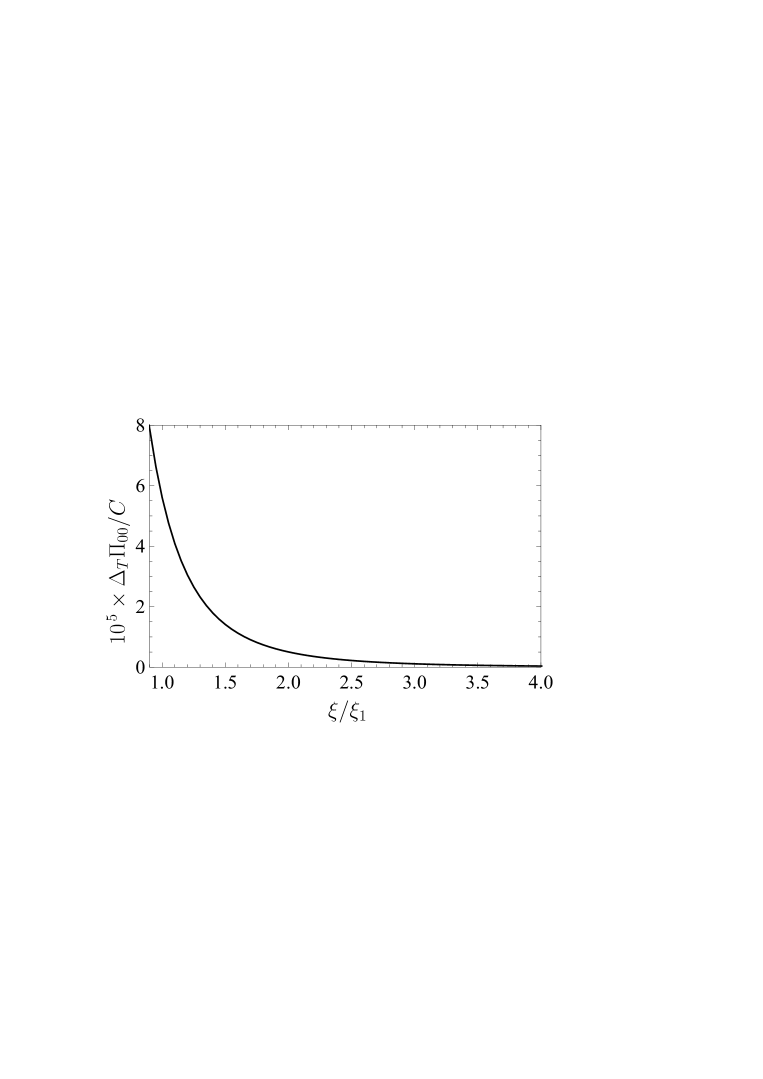
Figure 1: The normalized thermal correction to the 00-component of the polarization tensor of graphene computed as a function of the normalized imaginary frequency at $k_{\bot}=10\xi_{1}$ using the representation of Ref. 34.

As an illustration, in Fig. 1 we plot the thermal correction $\Delta_{T}\Pi_{00}(i\xi,k_{\bot})/C$ from Eq. (11), where the normalization factor is $C=16\alpha ck_{B}T/v_{F}^{2}$ and the frequency $\xi$ varies continuously along the imaginary frequency axis. The thermal correction is shown as a function of dimensionless variable $\xi/\xi_{1}$. The computations were performed for the gapless graphene ($\Delta=0$) at $T=300\,$K and $k_{\bot}=10\xi_{1}$. As is seen in Fig. 1, the thermal correction is a monotonously decreasing function of the frequency. Similar results hold at any temperature and transverse wave vector.

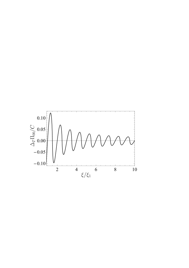
Figure 2: The normalized thermal correction to the 00-component of the polarization tensor of graphene computed as a function of the normalized imaginary frequency at $k_{\bot}=10\xi_{1}$ using the representation of Ref. 20.

For comparison purposes, in Fig. 2 we present the normalized thermal correction $\Delta_{T}\Pi_{00}(i\xi,k_{\bot})/C$ as a function of $\xi/\xi_{1}$, where the polarization tensor $\Pi_{kn}$ is taken from Ref. 20. The same values of $\Delta$, $T$ and $k_{\bot}$, as in Fig. 1, are used in computations. As is seen in Fig. 2, the function $\Delta_{T}\Pi_{00}(i\xi,k_{\bot})/C$ of Ref. 20 oscillates with the period equal to $2\pi/\xi_{1}$ and decreasing amplitude. At the points $\xi\equiv\xi_{l}=l\xi_{1}$ it takes the same values as the function $\Delta_{T}\Pi_{00}(i\xi,k_{\bot})/C$ of Ref. 34 (see Fig. 1), which are much smaller than the oscillation amplitudes. As a result, the analytic continuation of the function $\Delta_{T}\Pi_{00}(i\xi,k_{\bot})$ of Ref. 20 to the whole plane of complex frequencies becomes nonphysical.[34]

4 Origin of Large Thermal Effect for Graphene

The polarization tensor of graphene in combination with Eqs. (1) and (7) was used in many papers devoted to investigation of the Casimir effect in layered systems including graphene sheets. Specifically, the Casimir force between a graphene sheet and a material plate made of real dielectric or metal was investigated,[22] as well as between two graphene sheets.[24] The polarization tensor was also used to explore the Casimir-Polder interaction between different atoms and a graphene sheet[23, 26, 27] and the Casimir force between thin films[25] and graphene-coated substrates.[31]

The present section is devoted to the origin of thermal effect in the Casimir force for graphene which becomes dominant at much shorter separations than for ordinary materials. This origin can be investigated in the most straightforward way using the representation (11) and (13) for the polarization tensor. The point is that at all $l\geq 1$ and $T=300\,$K the expressions (11) and (13) are considerably simplified. Taking into account that $\xi_{1}\approx 2.4\times 10^{14}\,$rad/s and that the characteristic photon wave number, giving the major contribution to the Casimir free energy and pressure, is $k_{\bot}=1/(2a)$, one finds that at $a\geq 10\,$nm there is the natural small parameter

$$\frac{4v_{F}^{2}k_{\bot}^{2}}{c^{2}\tilde{q}_{l}^{2}}<\frac{4v_{F}^{2}k_{\bot}^{2}}{c^{2}\tilde{q}_{1}^{2}}\ll 1.$$ (15)

Expanding Eqs. (11) and (13) for the case $\Delta=0$ in powers of the small parameter (15), one obtains[35]

$$\Delta_{T}\Pi_{00}(i\xi_{l},k_{\bot})=\frac{\alpha\hbar k_{\bot}^{2}}{\tilde{q}_{l}}\,Y_{l},$$

$$\Delta_{T}\Pi(i\xi_{l},k_{\bot})={\alpha\hbar k_{\bot}^{2}}{\tilde{q}_{l}}Y_{l},$$ (16)

where

$$Y_{l}\equiv 4\int_{0}^{\infty}\frac{du}{e^{\pi lu}+1}\,\frac{u^{2}}{1+u^{2}}.$$ (17)

Using Eq. (9) for $\Delta=0$ and Eqs. (16), (8) and (7), one arrives at

$$r_{\rm TM}(i\xi_{l},k_{\bot})=\frac{\alpha q_{l}(\pi+Y_{l})}{\alpha q_{l}(\pi+Y_{l})+2\tilde{q}_{l}},$$

$$r_{\rm TE}(i\xi_{l},k_{\bot})=-\frac{\alpha\tilde{q}_{l}(\pi+Y_{l})}{\alpha\tilde{q}_{l}(\pi+Y_{l})+2{q}_{l}}.$$ (18)

Note that at $l=0$ the expressions (11) and (13) simplify considerably and their exact form is used in computations.[35]

We illustrate the precision of approximate expressions (18) in calculation of the Casimir pressure between two graphene sheets,

$$P(a,T)=-\frac{\partial{\cal F}(a,T)}{\partial a},$$ (19)

where ${\cal F}(a,T)$ is given in Eq. (1). In Fig. 3 we plot the quantity

$$\delta{P}^{(k)}(a,T)=\frac{{P}(a,T)-{P}^{(k)}(a,T)}{{P}(a,T)}$$ (20)

at $T=300\,$K, $\Delta=0$ as a function of separation, where $P(a,T)$ is computed exactly by Eqs. (1), (19), (7)–(13), $P^{(1)}(a,T)$ is computed using the approximate expressions (18) at $l\geq 1$ and $P^{(2)}(a,T)$ is computed by omitting the thermal correction to the polarization tensor at all $l\geq 1$, but replacing the continuous frequencies with the Matsubara ones[20] (the lines 1 and 2, respectively). As is seen in Fig. 3, the error arising from the use of approximate expressions (18) is negative and the maximum of its magnitude is equal to only 0.18%. At $a\geq 35\,$nm our calculation method[35] becomes practically exact. The error in the second approximate method[20] is positive and its maximum value is equal to 0.87%.

Figure 3: The relative errors of the approximate methods for calculation of the Casimir pressure between two graphene sheets using the asymptotic approach accounting for an explicit temperature dependence of the polarization tensor in all Matsubara terms (line 1) and disregarding this dependence in terms with $l\geq 1$ (line 2) are shown as functions of separation.

Now we are in a position to calculate different contributions to the thermal Casimir pressure between two graphene sheets with $\Delta=0$.

Figure 4: The normalized Casimir pressure between two graphene sheets at $T=300\,$K calculated at zero temperature (the lowest line), taking into account only an implicit temperature dependence (the intermediate line) and exactly (the upper line) are shown as functions of separation. The inset shows the region of short separations on an enlarged scale.

In Fig. 4 we plot the magnitudes of the Casimir pressure normalized to the quantity $B=k_{B}T/(8\pi a^{3})$ at $T=300\,$K as functions of separation. The lowest, intermediate and upper lines were computed at $T=0\,$K using the polarization tensor (9) with the continuous frequency $\xi$, at $T=300\,$K using the polarization tensor (9) with the discrete Matsubara frequencies, and at $T=300\,$K using the polarization tensor (11) and (13), respectively. In an inset the region of short separations is shown on an enlarged scale. Note that the same results for the upper line in Fig. 4 are obtained by using the approximate reflection coefficients given in Eq. (18). The total thermal correction is characterized by the difference of the upper and lowest lines in Fig. 4. It consists of the explicit thermal effect originating from the dependence of the polarization tensor on the temperature as a parameter (the difference between the upper and intermediate lines) and the implicit thermal effect originating from a summation over the temperature-dependent Matsubara frequencies (the difference between the intermediate and lowest lines).

As is seen in Fig. 4, the thermal effect quickly increases with increasing separation. At $a>150\,$nm it contributes more than 80% of the Casimir pressure. In so doing, the explicit thermal effect contributes more than the implicit one at the separations below 325 nm. At larger separations the implicit thermal effect dominates over the explicit one (this separation region is not shown in the figure). Thus, both contributions to the thermal correction in the Casimir pressure between two graphene sheets are important and should be taken into account.

5 Measuring of the Casimir Force for Graphene

The first experiment on measuring the gradient of the Casimir force between a Au-coated sphere and a graphene-coated substrate was performed[37] by means of a dynamic atomic force microscope (see Refs. 7 and 38 for a description of this measurement technique in application to the Casimir interaction). The sphere radius was $R=54.1\,\mu$m, and the graphene sheet was deposited on a 300 nm thick SiO₂ film covering a B-doped Si plate of $500\,\mu$m thickness.[37]

The gradient of the Casimir force in sphere-plate geometry can be calculated using the proximity force approximation as

$$\frac{\partial F_{sp}(a,T)}{\partial a}=2\pi R\frac{\partial{\cal F}(a,T)}{\partial a},$$ (21)

where the Casimir free energy per unit area in the configuration of two parallel plates is defined in Eq. (1). In this case the reflection coefficients $r_{\rm TM,\,TE}^{(1)}$ refer to a Au surface, whereas $r_{\rm TM,\,TE}^{(2)}$ describe the reflection properties of graphene deposited on a two-layer substrate. Both the reflectivity of Au and of a two-layer substrate can be easily expressed in terms of the frequency-dependent dielectric permittivities of Au, SiO₂ and Si. There was a problem, however, how to calculate the combined reflection coefficient of a two-dimensional graphene sheet, deposited on a three-dimensional substrate, where graphene is described by the polarization tensor and substrate materials by the dielectric permittivity. This problem was solved in Ref. 31 by the method of multiple reflections. The computations were performed using the polarization tensor with the nonzero mass gap parameter $\Delta\leq 0.1\,$eV taking into account that the graphene sheet could have the defects of structure and was deposited on a substrate.

The computed gradients of the Casimir force have been compared with the experimental data obtained in two series of measurements made for two graphene-coated plates over the separation region from 224 to 500 nm. A very good agreement between the measurement data and theory using the polarization tensor was demonstrated in the limit of experimental errors and theoretical uncertainties for both graphene samples. The experimental data was shown to be in complete disagreement with theoretical force gradients computed for the same substrate with no graphene coating.[37] The same measurement data were compared[33] with the alternative theoretical predictions obtained in the framework of the hydrodynamic model of graphene.[6, 7, 39] It was shown[33] that the hydrodynamic model is excluded by the measurement data at a 99% confidence level over the wide region of separations. Thus, the experiment of Ref. 37 can be considered as a confirmation of the Dirac model of graphene.

6 Possibility to Observe the Thermal Effect

The experiment[37] described in previous section has clearly demonstrated the influence of graphene coating on the Casimir interaction. In Ref. 32 the problem was raised on whether or not the same experimental data can be used as an evidence for large thermal effect in the Casimir interaction predicted for graphene at short separations.[8, 22, 24] To solve this problem, the gradients of the Casimir force $F_{sp}^{\prime}$ in the experimental configuration were computed as described above at $T=300\,$K and at $T=0\,$K taking into account all theoretical uncertainties.[32] It was shown that within the separation region from 224 to 300 nm the obtained theoretical bands do not overlap. The experimental data with their errors presented as crosses were shown to mostly belong to the theoretical band computed at $T=300\,$K (a few $\mu$N/m larger force gradients than at $T=0\,$K). Only several data crosses slightly touch the theoretical band at $T=0\,$K, which represents the force gradients with no thermal correction. This means that the already performed experiment[37] was only one step away from the conclusive observation of large thermal effect in the Casimir interaction between a Au-coated sphere and a graphene-coated substrate.

To solve a question as to whether the thermal effect is observable at the cost of a minor modification of the existing laboratory setup, the Casimir pressure between two parallel plates made of different materials was calculated, where at least one of the plates was coated with graphene.[32] Note that due to Eqs. (19) and (21), calculations of the Casimir pressure are equivalent to the calculations of the force gradients in the sphere-plate geometry, which is of an experimental interest.

The computations of the Casimir pressure were performed for the plates made of Au, Si, sapphire, mica and SiO₂. It was shown[32] that the influence of graphene coating (and of the thermal effect)is the most pronounced for a plate material having the smallest static dielectric permittivity (SiO₂). It is a happy accident that in the experiment of Ref. 37 just the amorphous SiO₂ (silica) satisfying this condition has been used as a material of the film underlying graphene. Then calculations of the thermal correction to the gradient of the Casimir force between a Au-coated sphere and a graphene-coated SiO₂ plate at the experimental separations have been performed. It was shown[32] that within the separation region from 224 to 350 nm the thermal correction markedly (up to a factor of five) exceeds the total experimental error. This makes the thermal effect observable if the thickness of a SiO₂ film is sufficiently large (computations were performed for a thick SiO₂ plate equivalent to a semispace).

Thus, the single point to be modified in the experiment of Ref. 37 is the thickness of a SiO₂ film which was equal to only 300 nm (see Sec. 5). If it were increased up to at least $2\,\mu$m (providing almost the same effect as a SiO₂ semispace) the large thermal effect in the gradient of the Casimir force originating from graphene would be observed with certainty.

7 Conclusions and Discussion

From the foregoing one can conclude that the Lifshitz theory and the formalism of the polarization tensor in (2+1)-dimensional space-time provide fundamental field-theoretical description of the Casimir interaction in layered systems containing graphene. The representation for the polarization tensor allowing the analytic continuation to the whole plane of complex frequencies can be also used to describe other physical phenomena, e.g., the reflectivities of graphene and graphene-coated substrates.[34, 40] This representation also leads to simple asymptotic expressions for the reflection coefficients at all nonzero Matsubara frequencies which result in nearly exact values for the Casimir energy and pressure. The developed theory is found to be in a very good agreement with the measurement data of the first experiment on measuring the gradient of the Casimir force between a Au-coated sphere and a graphene-coated substrate. In the framework of this theory the large thermal effect predicted for graphene earlier was shown to consist of two equally important parts originating from the parametric temperature dependence of the polarization tensor and from a summation over the Matsubara frequencies. It is shown that the thermal effect can be observed with already existing experimental setup if to make a minor modification of the used graphene sample.

In the future it is desirable to generalize the developed formalism for the case of nonzero chemical potential. This problem was recently solved,[41] but only for the case of gapless graphene.

References

- [1] M. I. Katsnelson, Graphene: Carbon in Two Dimensions (Cambridge University Press, Cambridge, 2012).
- [2] A. H. Castro Neto, F. Guinea, N. M. R. Peres, K. S. Novoselov and A. K. Geim, Rev. Mod. Phys. 81, 109 (2009).
- [3] M. I. Katsnelson, K. S. Novoselov and A. K. Geim, Nature Phys. 2, 620 (2006).
- [4] D. Allor, T. D. Cohen and D. A. McGady, Phys. Rev. D 78, 096009 (2008).
- [5] C. G. Beneventano, P. Giacconi, E. M. Santangelo and R. Soldati, J. Phys. A: Math. Theor. 42, 275401 (2009).
- [6] G. L. Klimchitskaya and V. M. Mostepanenko, Phys. Rev. D 87, 125011 (2013).
- [7] M. Bordag, G. L. Klimchitskaya, U. Mohideen and V. M. Mostepanenko, Advances in the Casimir Effect (Oxford University Press, Oxford, 2015).
- [8] G. Gómez-Santos, Phys. Rev. B 80, 245424 (2009).
- [9] J. F. Dobson, A. White and A. Rubio, Phys. Rev. Lett. 96, 073201 (2006).
- [10] M. Bordag, J. Phys. A: Math. Gen. 39, 6173 (2006).
- [11] M. Bordag, B. Geyer, G. L. Klimchitskaya and V. M. Mostepanenko, Phys. Rev. B 74, 205431 (2006).
- [12] D. Drosdoff and L. M. Woods, Phys. Rev. B 82, 155459 (2010).
- [13] D. Drosdoff and L. M. Woods, Phys. Rev. A 84, 062501 (2011).
- [14] T. E. Judd, R. G. Scott, A. M. Martin, B. Kaczmarek and T. M. Fromhold, New. J. Phys. 13, 083020 (2011).
- [15] J. Sarabadani, A. Naji, R. Asgari and R. Podgornik, Phys. Rev. B 84, 155407 (2011).
- [16] Bo E. Sernelius, Europhys. Lett. 95, 57003 (2011).
- [17] Bo E. Sernelius, Phys. Rev. B 85, 195427 (2012).
- [18] A. D. Phan, L. M. Woods, D. Drosdoff, I. V. Bondarev and N. A. Viet, Appl. Phys. Lett. 101, 113118 (2012).
- [19] M. Bordag, I. V. Fialkovsky, D. M. Gitman and D. V. Vassilevich, Phys. Rev. B 80, 245406 (2009).
- [20] I. V. Fialkovsky, V. N. Marachevsky and D. V. Vassilevich, Phys. Rev. B 84, 035446 (2011).
- [21] Yu. V. Churkin, A. B. Fedortsov, G. L. Klimchitskaya and V. A. Yurova, Phys. Rev. B 82, 165433 (2010).
- [22] M. Bordag, G. L. Klimchitskaya and V. M. Mostepanenko, Phys. Rev. B 86, 165429 (2012).
- [23] M. Chaichian, G. L. Klimchitskaya, V. M. Mostepanenko and A. Tureanu, Phys. Rev. A 86, 012515 (2012).
- [24] G. L. Klimchitskaya and V. M. Mostepanenko, Phys. Rev. B 87, 075439 (2013).
- [25] G. L. Klimchitskaya and V. M. Mostepanenko, Phys. Rev. B 89, 035407 (2014).
- [26] G. L. Klimchitskaya and V. M. Mostepanenko, Phys. Rev. A 89, 012516 (2014).
- [27] G. L. Klimchitskaya and V. M. Mostepanenko, Phys. Rev. A 89, 062508 (2014).
- [28] B. Arora, H. Kaur and B. K. Sahoo, J. Phys. B 47, 155002 (2014).
- [29] K. Kaur, J. Kaur, B. Arora and B. K. Sahoo, Phys. Rev. B 90, 245405 (2014).
- [30] G. L. Klimchitskaya, V. M. Mostepanenko and Bo E. Sernelius, Phys. Rev. B 89, 125407 (2014).
- [31] G. L. Klimchitskaya, U. Mohideen and V. M. Mostepanenko, Phys. Rev. B 89, 115419 (2014).
- [32] G. L. Klimchitskaya and V. M. Mostepanenko, Phys. Rev. A 89, 052512 (2014).
- [33] G. L. Klimchitskaya and V. M. Mostepanenko, Phys. Rev. A 91, 045412 (2015).
- [34] M. Bordag, G. L. Klimchitskaya, V. M. Mostepanenko and V. M. Petrov, Phys. Rev. D 91, 045037 (2015).
- [35] G. L. Klimchitskaya and V. M. Mostepanenko, Phys. Rev. A 91, 174501 (2015).
- [36] S. J. Rahi, T. Emig, N. Graham, R. J. Jaffe and M. Kardar, Phys. Rev. D 80, 085021 (2009).
- [37] A. A. Banishev, H. Wen, J. Xu, R. K. Kawakami, G. L. Klimchitskaya, V. M. Mostepanenko and U. Mohideen, Phys. Rev. B 87, 205433 (2013).
- [38] G. L. Klimchitskaya, U. Mohideen and V. M. Mostepanenko, Rev. Mod. Phys. 81, 1827 (2009).
- [39] G. Barton, J. Phys. A: Math. Gen. 38, 2997 (2005).
- [40] G. L. Klimchitskaya, C. C. Korikov and V. M. Petrov, Phys. Rev. B 92, 125419 (2015).
- [41] M. Bordag, I. V. Fialkovsky and D. V. Vassilevich, Enhanced Casimir effect for doped graphene, arXiv:1507.08693.