Which Way?

Abstract

I report the result of a which-way experiment based on Young’s double-slit experiment. It reveals which slit photons go through while retaining the (self) interference of all the photons collected. The idea is to image the slits using a lens with a narrow aperture and scan across the area where the interference fringes would be. The aperture is wide enough to separate the slits in the images, i.e., telling which way. The illumination pattern over the pupil is reconstructed from the series of slit intensities. The result matches the double-slit interference pattern well. As such, the photon’s wave-like and particle-like behaviors are observed simultaneously in a straightforward and thus unambiguous way. The implication is far reaching. For one, it presses hard, at least philosophically, for a consolidated wave-and-particle description of quantum objects, because we can no longer dismiss such a challenge on the basis that the two behaviors do not manifest at the same time. A bold proposal is to forgo the concept of particles. Then, Heisenberg’s uncertainty principle would be purely a consequence of waves without being ordained upon particles.

Day Month Year

PACS numbers: 03.65.Ta; 42.25.Hz; 42.50.Xa.

1 Complementarity and Particle-Wave Duality

The principle of complementarity states that complementary properties of a quantum object cannot be observed simultaneously. A commonly cited example is that particles can either exhibit particle behavior or wave behavior in an experiment but not both at the same time. This is at the heart of particle-wave duality. Because complementarity cannot be derived from first principle, it is regarded by many a fundamental principle of quantum mechanics.

There are still many who wish to test complementarity. Take Young’s double-slit experiment as an example. One would try to determine which slit each photon goes through (i.e., which-way information) and obtain the interference fringes at the same time. Along the development, it was realized that one may obtain some which-way information at the expense of reduced sharpness of the interference. Furthermore, the sum of which-way and interference information should not exceed the maximum available in the experiment,[1, 2, 3] which, for instance, equals the amount of information in absolutely accurate slit determination (thus no fringes at all) or complete ignorance of the slit information (thus full interference). An inequality in terms of the fringe visibility ($\mathcal{V}$) and the slit or path distinguishability ($\mathcal{D}$) was later introduced:[4, 5, 6]

$$\mathcal{V}^{2}+\mathcal{D}^{2}\leq 1.$$ (1)

Operationally, $\mathcal{V}$ represents the fringe contrast, and $\mathcal{D}$ is the normalized likelihood, in excess of a uniform random guess, of determining the slit correctly. More quantitative definitions are given in sections 2 and 3.

One can find a number of which-way experiments in the literature (for a few recent examples, see Refs. kocsis2011,menzel2012), though conclusive evidence of violation of complementarity has yet to be established. Chris Stubbs told me about Afshar’s experiment[9] while I was finishing this article. Both Afshar’s experiment and mine image the double openings (pinholes or slits) to determine the photons’ path, but the rest are different. In the former, a grid of thin wires are placed before the lens lying where the dark fringes of the double pinholes would be. The image of the pinholes is only slightly affected by the wires, showing that the wires block and diffract only a small amount of light. It is thus consistent with the wires being where the dark fringes would be. However, imagine placing a much thinner wire where a bright fringe would be. Much like dust on the primary mirror of a telescope, such a wire could easily escape detection in the image of the pinholes, which means that one cannot accurately determine the illumination pattern over the lens without perturbing the pinhole image significantly. Moreover, as pointed out in section 4.4, it is not possible to reconstruct the illumination pattern from just one image of the double pinholes. Therefore, without a precise match of the illumination pattern with the interference pattern, Afshar’s experiment is not a sufficient proof of violation of complementarity.

Before describing my experiment, it is worth reading some thoughts of Bohr who first introduced the principle of complementarity in 1927. In the key paper published the following year, Bohr remarked on the wave behavior of matter after similar comments on that of light:[10]

In fact, here again we are not dealing with contradictory but with complementary pictures of the phenomena, which only together offer a natural generalisation of the classical mode of description.

I imagine that Bohr was concerned about the challenge of particle-wave contradiction to the foundation of quantum mechanics. Complementarity seemed to be a necessary way out but not a satisfactory one by itself. Given that a proof from first principle was not possible, it was imperative to establish support of some physical origin for complementarity. Bohr found a solution in the physics of measurements, which helped secure complementarity and turned the contradiction into duality. With loose ends tied up, he concluded the very paper with

I hope, however, that the idea of complementarity is suited to characterise the situation, which bears a deep-going analogy to the general difficulty in the formation of human ideas, inherent in the distinction between subject and object.

What if there are no particles but only waves?

2 Seeing the Slits

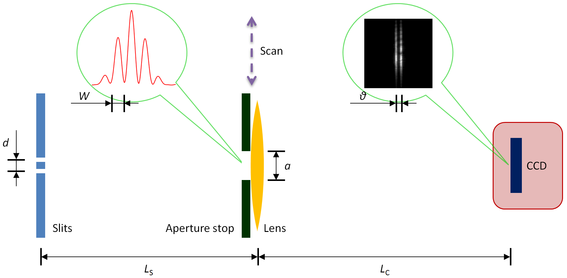
Figure 1: Experiment design.

While contemplating ways to circumvent complementarity, I imagined myself looking at a double-slit mask. Then, I knew how to trick the photons. Like seeing the two slits with the naked eye, the illuminated slits can be imaged with a camera as illustrated in Fig. 1. But here comes an important question: would the photon stop interfering with itself as it arrives at the lens?

If the detector is placed right behind the thin lens, it still registers the interference pattern with slight optical effects. Only when the distance between the lens and the detector and that between the lens and the slits roughly satisfy the lens equation does one get an image of two distinct slits. A perfect image of the slits does not reveal whether the photon interferes with itself or not just before hitting the lens. If it did not, however, then some long-range interaction would be needed to inform the photon of the details of the apparatus ahead (e.g., lens or screen, curvature of the lens, position of the detector, etc.) so that it can react accordingly before entering the lens. Neither electromagnetic interaction nor gravitational interaction could accomplish this. Introducing a new long-range force can potentially facilitate information delivery but cannot evade the memory problem discussed in section 4.2. Therefore, my answer to the question above is “no.”

There is still a technical problem of well resolving the slits on the detector and the fringes at the lens simultaneously. The hypothesis here is that the illumination pattern over the lens (more appropriately, the pupil) should be the same as the double-slit interference pattern, so in order to properly reconstruct the former the experiment should be capable of resolving the fringes at the position of the lens. The characteristic scale $W$ of the fringes is given by

$$W=\frac{\lambda}{d}L_{\mathrm{S}},$$ (2)

where $\lambda$ is the photon’s wavelength, $d$ is the separation between the two slits, and $L_{\mathrm{S}}$ is the distance between the slits and the lens. The two slits subtend an angle $\theta\simeq d/L_{\mathrm{S}}$ to the lens. The angular resolution of the imaging part is roughly $\lambda/a$ with $a$ being the aperture width. Now there are two conflicting requirements. On one hand, the aperture width should be much smaller than $W$ to resolve the fringes well, i.e.,

$$a\ll W\ \ \mbox{or}\ \ a\ll\frac{\lambda}{d}L_{\mathrm{S}}.$$ (3)

On the other hand, separating the two slits in the images demands the opposite (barely resolving the two slits is not sufficient to separate them to satisfaction), i.e.,

$$\frac{\lambda}{a}\ll\theta\ \ \mbox{or}\ \ a\gg\frac{\lambda}{d}L_{\mathrm{S}}.$$ (4)

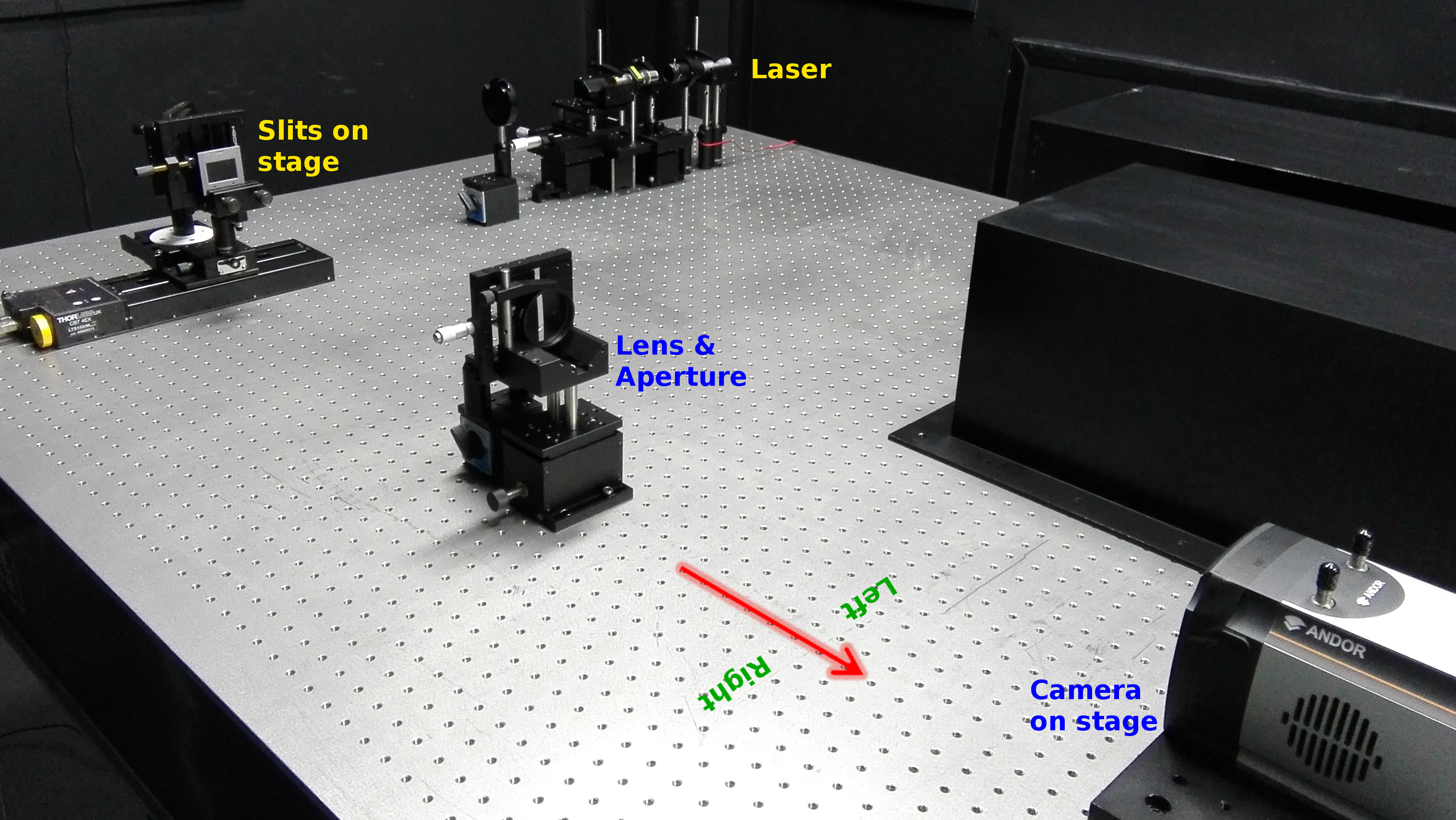
Figure 2: Experiment setup.

For a moment, I thought quantum mechanics guarded its secret well. Then the technique of drizzling[11] came to my mind, which enhances the image resolution by properly combining several undersampled images taken with sub-pixel dithering. Drizzling was developed for Hubble Space Telescope and has become a standard practice in astronomy. It works because a pixel has fairly sharp boundaries capable of sampling spatial frequencies higher than the pixel Nyquist frequency. Hence, it is feasible to properly reconstruct the illumination pattern from a series of scans over the pupil plane in fine steps, even if the aperture is wider than the fringes. One might argue that since the slit images are taken at different times, it does not qualify for a simultaneous observation of the particle and the wave behaviors. A conceptual solution is to use a large number of beam splitters, lenses, aperture stops, and cameras to achieve the same effect of the scan while observing the slits simultaneously.

The experiment is prepared as shown in Fig. 2. A red laser diode is used as the coherent light source. Its central wavelength is not precisely known, so a $650\,\mbox{nm}$ filter (bandwidth $10\,\mbox{nm}$) is added for the sole purpose of providing a definitive wavelength to work with. A spatial filter is set up to improve the beam quality. The double-slit mask appears to be a film negative. The width ($\delta$) of each slit and the center-to-center distance ($d$) between the two slits are $89\,\mu\mbox{m}$ and $248\,\mu\mbox{m}$, respectively, measured from a non-contact surface scan over a small section of the mask (see Fig. 3). The aperture stop is an adjustable mechanical slit with a micrometer to determine its width. It is placed as close to the lens as possible and opens in one direction, toward the right. The left and right directions on the air bearing table are defined as one looks along the direction of propagation of the photons, so that they are consistent with those on the images taken by the camera. An example is given in Fig. 2. The lens has a nominal focal length of $300\,\mbox{mm}$. The camera (Andor DU934P) is equipped with a $1024\times 1024$ back-side illuminated deep depletion CCD whose pixel size is $13\,\mu\mbox{m}\times 13\,\mu\mbox{m}$. At the readout rate of $1\,\mbox{MHz}$, the readout noise is roughly $6\,\mbox{e}^{-}$ per pixel.

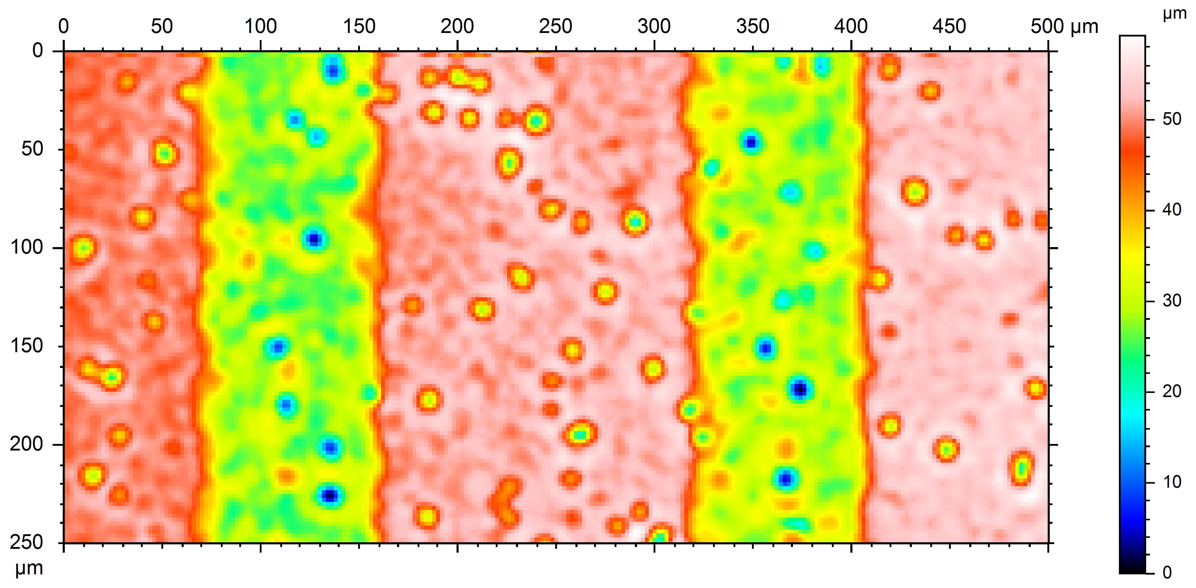
Figure 3: Surface height of a small section of the double-slit mask.

Perturbations to the lens and the aperture stop are likely to have a larger effect than those to the double-slit mask. Hence, instead of moving the former in the conceptual design of Fig. 1, I mount the double slits on a motorized stage (Thorlabs LTS150) with a minimum repeatable incremental movement of $4\,\mu\mbox{m}$ and a calibrated absolute on-axis accuracy of $\pm 5\,\mu\mbox{m}$. The distance between the slits and the lens is $L_{\mathrm{S}}\simeq 58\,\mbox{cm}$, and that between the lens and the camera is $L_{\mathrm{C}}\simeq 63\,\mbox{cm}$. These distances are not accurately measured. The camera is mounted on another motorized stage (Thorlabs LTS300), which has the same specifications as the first one except for a travel range twice as long. The two stages move in the opposite direction at a ratio of $1:1.07$, so that the slits stay at the center of the detector. In this way, it is not necessary to flat-field the camera, and the slits and their diffraction wings from the aperture stop remain on the detector through out a scan of $30\,\mbox{mm}$ across the illumination pattern.

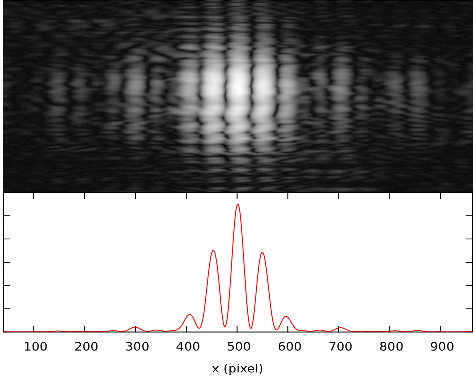
Figure 4: Upper panel: A reference-subtracted and stacked image of the double-slit interference pattern. The greyscale is logarithmic. Lower panel: The mean flux in each column of the pixels in the image above.

For comparison with the reconstructed result in section 3, the double-slit interference pattern is imaged at approximately $D\simeq 25\,\mbox{cm}$ from the slits. Fig. 4 displays an average of 110 frames of the fringes with the mean of 105 reference images subtracted. The references are obtained in the same way as the fringe images are in all aspects except that the laser is switched off. The subtraction removes the bias, dark current, and darkroom background at the same time. The process of reference subtraction is applied to all the images in this work, and it is no longer mentioned hereafter. The fringes do not look as good as one would like because of the low quality of the slits (evident in Fig. 3) and that of the laser beam. Nevertheless, the column-averaged fringe profile is satisfactory.

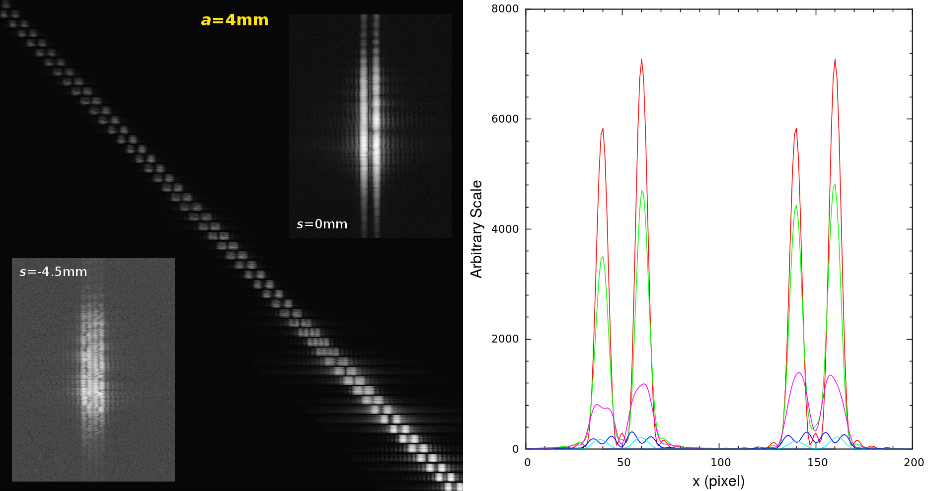
Figure 5: Left panel: Vertically binned and cut-out images of the double slits at every third step in the scan sequence with the aperture width $a=4\,\mbox{mm}$. The top row and the bottom row correspond to the slits at $s=-15$ and $0\,\mbox{mm}$, respectively. The results are roughly symmetric around the origin, so the right half of the scan is omitted. The horizontal shift between consecutive rows is reduced to keep all the slit images within the panel. The insets show the full images taken at $s=0\,\mbox{mm}$, where the slits are well resolved, and $s=-4.5\,\mbox{mm}$, where the slits are barely separated. The greyscales of the insets and the main image are all logarithmic. Right panel: Column-averaged intensity profiles of the slit images. From top to bottom, the ones centered at $x=50\,\mbox{pix}$ correspond to the images taken at $s=0$, $1.5$, $3$, $4.5$, and $6\,\mbox{mm}$; the ones centered at $x=150\,\mbox{pix}$ correspond to $s=0$, $-1.5$, $-3$, $-4.5$, and $-6\,\mbox{mm}$.

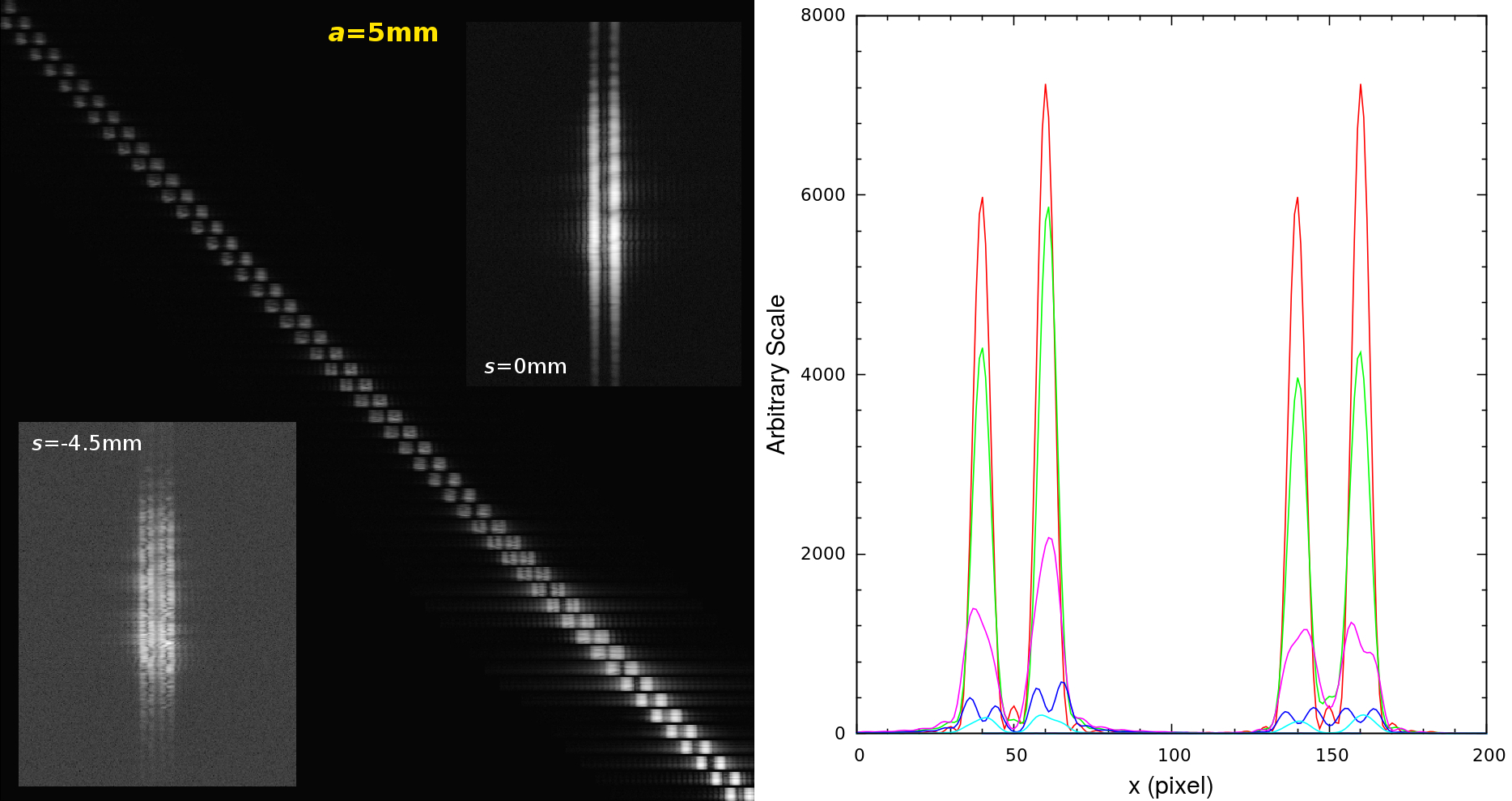
Figure 6: Same as Fig. 5 but for the aperture width of $a=5\,\mbox{mm}$.

Two scans are performed, one with an aperture width of $a=4\,\mbox{mm}$ and the other with $a=5\,\mbox{mm}$. The slits move from left ($s=-15\,\mbox{mm}$) to right ($s=15\,\mbox{mm}$), or, equivalently, the illumination pattern is scanned from right to left. The step size is $\Delta s=0.1\,\mbox{mm}$, much smaller than the characteristic scale of the fringes at a distance of approximately $58\,\mbox{cm}$ from the slits. Four images are taken and averaged at each step. The optical axis of the lens marks the nominal “zero” position of the slits and that of the camera. The exposure time is adjusted to the aperture width so that no pixel is close to saturation, and it remains the same throughout each scan. Samples of the slit images and column-averaged intensity profiles are shown in Fig. 5 ($a=4\,\mbox{mm}$) and Fig. 6 ($a=5\,\mbox{mm}$). The separation between the two slits in the images is roughly 20 pixels or $243\,\mu\mbox{m}$ in the plane of the slits, consistent with the slit separation measured from Fig. 3.

Tagging each photon with a slit is an intrinsically probabilistic matter. A photon passing one of the slits can land in any pixel on the detector that is allowed by diffraction of the aperture stop, which is indeed seen in the images. As such, an a posteriori probability should be assigned to the photon going through a particular slit based on the location on the detector where it is registered. An accurate quantitative analysis is not the main concern of this work. It suffices to obtain a rough lower bound of the slit distinguishability for testing the inequality in Eq. (1).

Since the slits are reversed in the images, the flux to the left (right) of the midline between the two slits in the images should be assigned to the right (left) slit. To avoid confusion between the slits and their images, I refer to the flux to the left (right) of the midline as the left (right) signal. Clearly, a small fraction of the photons would be assigned incorrectly. Since the intensity profile of each slit in the images is roughly symmetric around its center and since the distance from the midline to the center of either slit in each image is about 10 pixels, the amount of contamination to the left (right) signal would not exceed the total flux more than 20 pixels away to the right (left) of the midline. The total contamination as a fraction of the total signal is thus $5.1\%$ for the scan with the aperture width of $a=4\,\mbox{mm}$ and $4.2\%$ for $a=5\,\mbox{mm}$. This means that the probability ($p$) of correct slit assignment is greater than $0.95$. The slit distinguishability is defined as[4]

$$\mathcal{D}=\left(\frac{1}{2}\right)^{-1}\left(p-\frac{1}{2}\right).$$ (5)

Hence, this experiment achieves $\mathcal{D}\geq 0.9$.

The difference between Fig. 5 and Fig. 6 may not be obvious to the eye, but the insets show narrower and more compact diffraction patterns with the latter as a result of the wider aperture width in use. A further increase of the aperture width is likely to better separate the slits. However, I suspect that beyond a certain size that is determined by the double-slit interference pattern at the aperture stop there would be no more gain from increasing the aperture width, because the pupil is not uniformly illuminated. It also means that the diffraction patterns in Figs. 5 and 6 cannot always be described by single-slit diffraction. When they can, it is likely that the two edges of the aperture stop are equally illuminated. Another idea of improvement comes from starshade[12], which suppresses diffracted light by apodizing the sharp edge that cuts into the light ray.

3 Reconstructing the Interference

The total flux recorded by the camera at each step ($F$) is proportional to that passing through the aperture stop. The proportional constant is the system efficiency and is irrelevant in this work. In a discrete representation, the relation reads

$$F=AP,$$ (6)

where $P$ is the illumination pattern over the pupil (operationally, it is a vector of flux values at the aperture stop in fine intervals), and $A$ is a matrix summing $P$ inside the aperture to produce the measured flux $F$ at each step (hereafter, it is referred to as the aperture matrix). The task is to recover $P$ from $F$. Since $P$ cannot contain any useful information at spatial frequencies higher than those in $F$, the physical interval between two consecutive elements in $P$ should not be smaller than the step size of the scans, i.e., the reconstructed illumination pattern cannot have a resolution finer than that of the scans.

A problem arises immediately from the dimensions. One may assume that the illumination faraway from the center is too low to affect the reconstruction and truncate $P$ to a finite length. But the recorded flux vector $F$ would still have less elements than $P$, and the difference in physical units is the width of the aperture. This means that $P$ cannot be uniquely determined from $F$. To proceed, I truncate $P$ further to match the length of $F$. The associated error in reconstruction should decrease as one increases the physical length of the scans.

Since the scans are carried out in 301 steps at intervals of $\Delta s=0.1\,\mbox{mm}$, the recorded flux $F$, the recovered illumination pattern $P$, and the aperture matrix $A$ have dimensions of 301 or $301\times 301$ as appropriate. The aperture widths of $4\,\mbox{mm}$ and $5\,\mbox{mm}$ then correspond to 40 and 50 elements in $A$, respectively, i.e.,

$$A_{ij}(4\,\mbox{mm})=\left\{\begin{array}[]{lc}1&\quad i-20<j\leq i+20\\ 0&\quad\mbox{else}\end{array}\right.$$ (7)

and

$$A_{ij}(5\,\mbox{mm})=\left\{\begin{array}[]{lc}1&\quad i-20<j\leq i+30\\ 0&\quad\mbox{else.}\end{array}\right.$$ (8)

The same condition “$i-20<j$” appears in both Eq. (7) and Eq. (8) because the aperture stop opens toward the right.

A straightforward way to obtain the illumination at the aperture stop as a function of position in the scan direction is to solve Eq. (6). It turns out that the aperture matrix $A(4\,\mbox{mm})$ is full rank only if its dimensions are multiples of 40 or those plus one, e.g., 40, 41, 80, 81, and so on. Similarly, the magic numbers for $A(5\,\mbox{mm})$ are 50, 51, 100, 101, and so on. The dimensions of $301\times 301$ would not allow a unique determination of $P$ with $A(4\,\mbox{mm})$, but the degeneracy can be lifted by incorporating $A(5\,\mbox{mm})$:

$$\hat{P}=\begin{bmatrix}A(4\,\mbox{mm})\\ A(5\,\mbox{mm})\end{bmatrix}^{+}\begin{bmatrix}F(4\,\mbox{mm})\\ F(5\,\mbox{mm})\end{bmatrix},$$ (9)

where the symbol “+” denotes pseudoinverse, and the measured fluxes through the aperture stop have been scaled by their exposure times. Eq. (9) is essentially a least-square estimate of $P$.

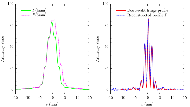
Figure 7: Left panel: The measured fluxes as functions of the position in the scan sequence for the aperture widths $a=4\,\mbox{mm}$ (solid line) and $a=5\,\mbox{mm}$ (dotted line). Right panel: The profile of the double-slit interference pattern from Fig. 4 (solid line) and that of the reconstructed illumination pattern $\hat{P}$ (dotted line) from the measured fluxes in the left panel. The reconstructed profile has been smoothed with a Gaussian kernel that has an rms of $0.15\,\mbox{mm}$.

The measured fluxes with the aperture widths $a=4\,\mbox{mm}$ (solid line) and $5\,\mbox{mm}$ (dotted line) are shown in the left panel of Fig. 7. As a combined result of the $1\,\mbox{mm}$ difference between the aperture widths and the fact that the characteristic width $W$ of the fringes at the aperture stop is a few times (but not much) narrower than the aperture widths, the flux profile $F(5\,\mbox{mm})$ is roughly $1\,\mbox{mm}$ wider than $F(4\,\mbox{mm})$. The profile of the reconstructed illumination pattern $\hat{P}$ (dotted line) is presented in the right panel of Fig. 7 along with that of the directly imaged fringe profile scaled from Fig. 4 (solid line). The horizontal scaling factor equals $0.030\,\mu\mbox{m}/\,\mbox{pix}$, which is the pixel size ($13\,\mu\mbox{m}$) multiplied by the ratio of the distance between the slits and the lens ($L_{\mathrm{S}}\simeq 58\,\mbox{cm}$) to that between the slits and the camera ($D\simeq 25\,\mbox{cm}$) when the interference pattern is directly imaged. The vertical scaling is determined by matching the height of the central peaks of the two profiles. The only parameter that is free to adjust is the horizontal shift between the two curves. It is remarkable that the two profiles match well in the central region without any other tweaks. I would like to mention that even a slight alteration to the aperture matrix, e.g., misrepresenting the aperture widths by just one element ($0.1\,\mbox{mm}$ in physical units), or mis-aligning one aperture with respect to the other by one element, would result in fairly noticeable deterioration to the reconstructed illumination pattern.

The reconstruction is not reliable in the outskirts, where the flux level is low. The high-frequency ripples that are conspicuous on the left side bear the characteristic period of $1\,\mbox{mm}$, which is the difference between the two aperture widths. I expect that much improvement can be achieved with better instruments, more sampling (e.g., longer scans, more aperture widths, and finer steps), and better control of the laboratory environment.

For interferometry experiments, the fringe visibility is given by the contrast of the fringes[4]

$$\mathcal{V}=\frac{I_{\mathrm{max}}-I_{\mathrm{min}}}{I_{\mathrm{max}}+I_{\mathrm{min}}},$$ (10)

where $I_{\mathrm{max}}$ and $I_{\mathrm{min}}$ are, respectively, the maximum and minimum intensities of the fringes. The double-slit interference fringes are modulated by diffraction of individual slits. As the width of each slit of the double slits decreases, more and more fringes will become similar to the one in the center, and eventually they will resemble interferometric fringes. Therefore, it is reasonable in this experiment to use the contrast of the reconstructed central peak and troughs to calculate the visibility. To be conservative, I estimate $\mathcal{V}$ with the second and third peaks and the troughs between them in Fig. 7. The result is $\mathcal{V}\geq 0.69$, and with $\mathcal{D}\geq 0.90$ from section 2 one finds $\mathcal{D}^{2}+\mathcal{V}^{2}\geq 1.3$. The inequality in Eq. (1) is thus violated with a wide margin. It is worth mentioning that the fringe visibility is naturally reduced by unequal illumination of the two slits as seen in Figs. 5 and 6.

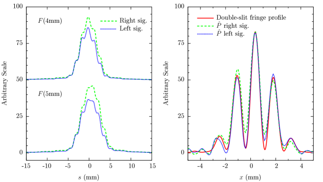
Figure 8: Same as Fig. 7 but showing results separately for photons going through mostly the left slit (dashed lines) and those through mostly the right slit (dotted lines). The fluxes $F(4\,\mbox{mm})$ in the left panel are shifted vertically for clarity.

By now one would be eager to see if there is any difference between the reconstructed illumination pattern of the photons going through the left slit and that of the photons going through the right slit. The left panel of Fig. 8 displays the right signals (dashed lines) and the left signals (dotted lines) of the two scans as calculated in section 2. It is understood that the left (right) signal contains mostly photons going through the right (left) slit with slight contamination from photons through the other slit. The right signals are higher than the left signals, because the two slits are not illuminated equally. The profile of the reconstructed illumination pattern from the right signal (dashed line) and that from the left signal (dotted line) are shown in the right panel of Fig. 8. The profiles are still normalized by their central peaks. The most important feature is that the two profiles are more or less the same. However, it does not mean that a single slit could produce the double-slit interference pattern. It merely corroborates what is shown in the left panel of Fig. 8: the two slits make similar contributions to the illumination pattern everywhere across the pupil, albeit minor differences in shape and a more pronounced one in the overall intensity mentioned above.

The right panel of Fig. 8 displays an asymmetry between the reconstructed illumination pattern from the left signal and that from the right signal. Further work is needed to determine whether it is a feature of physical significance or merely a result of an imperfect setup of the experiment.

4 Discussion

My experiment demonstrates that one can determine at the same time which slit the photons go through with high confidence and recover an illumination pattern that matches the double-slit interference pattern. A rough estimate of the fringe visibility and the slit distinguishability suggests that the principle of complementarity is violated. This result brings up a challenging question: what is particle-wave duality? It seems that a simple solution to the conundrum is to forgo the concept of particles.

4.1 Ambivalent Identities

Although particle-wave duality is deeply entrenched in our minds, it seems that the particle aspect and the wave aspect are always discussed in different realms. There lacks a complete theory to explain the mechanism of particle-wave duality. It also appears that quantum mechanical calculations do not require mathematical constructs specific to the particle nature to describe particles. In my observation, the concept of particles is needed only when detection or related processes (e.g., the photoelectric effect) are involved.

But, what is the defining property of a particle as opposed to a wave? I consider a particle to be an entity of a finite and more-or-less fixed size in its rest frame. A reasonable extension is that a particle is discrete and impermeable unless being broken into. Consequently, a particle cannot go through both slits in Young’s double-slit experiment. This is the root cause of contradiction between the particle and the wave behaviors. From daily experience, a wave is permeable and often propagating into as much space as possible. These properties do not hold fast. Even though calculations show that the degeneracy pressure of wave functions can build the stiffest objects in the universe, we still prefer subconsciously that we are made of particles rather than waves.

A photon is always detected by a localized event, so it is natural to consider the photon as a particle. Being a particle, the photon has to choose only one slit to go through. Even the thought of a photon going through one of the slits is deeply disturbing – how could the simple photon sense and react to the other slit at a macroscopic distance away from itself? The epistemic doctrine of “measurement of the particle behavior of a quantum object impairs the measurement of its wave behavior” circumvents the issue, but to some it is not satisfactory.

4.2 Paving the Wave

The photon-counting version of Young’s double-slit experiment could have pushed the particle-wave dilemma to the frontstage. However, it was not designed to reveal the trajectories of the photons, which is considered the ultimate test of their particle nature.

The scenario of self-interference was proposed to account for the result of the photon-counting double-slit experiment, but there are difficulties. Firstly, one still has to answer the question of how the existence of the second slit affects the photon’s behavior. The question can be rephrased as “would properties specific to the particle nature be required in a theory that explains the interaction between the photon and the two slits?” Secondly, what is the difference between a photon traveling in free space and a photon going through one of the two slits (or through the only slit in a single-slit experiment, which could also invoke self-interference)? How does the photon know whether it should interfere with itself or not? If it should, then where (or when) should self-interference happen? It cannot occur right behind the slits, because no fringes but a projection of the two slits can be seen on a screen there. Along this line, one soon reaches a memory problem: if the photon decides whether to interfere with itself according to its past, then it needs a mechanism to store the information, which could be arbitrarily complex in both spatial dimensions (e.g., openings in arbitrary shapes and numbers) and the time dimension (e.g., arbitrary number of consecutive slits). It does not seem possible that a particle as simple as the photon can memorize an infinite history.

Waves do not suffer from the memory problem. Information can be carried in the wave form, which would be a function of spatial coordinates, momentum, and time. The wave form would be altered by the apparatus along the way, analogous to the wavefront in optics. The difference between a photon going through double slits and another one through a single slit would be solely in the wave form after they pass their respective slit masks. Since the photon wave could span across the two slits, there is no need to invent a new type of interaction for the wave to sense both slits. It would just be reconditioned by the slits. Waves can evolve while propagating, so some distance after the slits would be needed for fringes to develop.

Strictly speaking, we do not detect photons directly, not even with eyes; we only detect very localized effects of photons. Such detection ultimately involves absorption, which is accurately described by the interaction between two fields in quantum electrodynamics: a radiation field and a bound charged particle field without requiring representations specific to the particle nature (let us hold the question of whether electrons, protons, etc. are particles for the moment). Therefore, a pixel registering a photon, no matter how small the pixel is, is not a sufficient proof that the photon is a particle.

One would still wonder, if the photon is really a wave that can spread over a large area, how can it hit just a single pixel? We might borrow the idea of wave function collapse in quantum measurement theory, but I think much work is needed to fully understand the process of collapsing. My conjecture is that once the photon wave arrives at the detector, the best matching atom (wave) would absorb the photon in a runaway process, excluding the possibility of being absorbed by another atom elsewhere at the same time. The atoms in the detector would be in random phases, so they would sample the photon wave at random individually but still produce the double-slit fringes collectively. If no atom is ready to absorb the photon, reflection or transmission occurs. This scenario can be interesting when identical targets are prepared coherently.

4.3 The Photoelectric Hurdle

It is widely accepted that the photoelectric effect anchors the particle nature of the photon. Since it is an absorption process, the same argument in section 4.2 applies. However, it is worth delving a bit deeper and even digressing a little.

Let us start with a quote from a translation of Einstein’s words[15, 16]:

…it is quite conceivable that a theory of light involving the use of continuous functions in space will lead to contradictions with experience, if it is applied to the phenomena of the creation and conversion of light.
…when a light ray starting from a point is propagated, the energy is not continuously distributed over an ever increasing volume, but it consists of a finite number of energy quanta, localised in space, which move without being divided and which can be absorbed or emitted only as a whole.

The above statement assumes that a continuous function must behave continuously in all aspects. It need not be so. The wave function of a particle in a box is continuous, but its energy is discrete, proportional to $n^{2}m^{-1}$, where $n$ is a positive integer, and $m$ is the particle mass. If we drop the concept of particles here, then the mass is just another parameter of the wave (function) much like the wavelength of the photon. Such waves can only exchange discrete amounts of energy in interactions with each other. Since, unlike the radiation field, photons themselves do not have excitation states, we can make an analogy between them and the ground-state wave ($n=1$) in the box with the photon energy controlled by its wavelength rather than mass. If a photon wave is ever absorbed by another wave, the latter has to take all the energy of the former as a whole.

Contrary to common believes, classical physics would practically prohibit the photoelectric effect if energy is continuously imparted on electrons in a metal. Let me use industrial CO₂ lasers as an example. They can easily reach a power density of $10^{12}\,\mbox{W}\,\mbox{m}^{-2}$, far powerful than any light source obtainable in the 1900s; for comparison, the solar constant is a feeble $1361\,\mbox{W}\,\mbox{m}^{-2}$. Assuming that the lattice size of the metal is roughly $5\,\mbox{\AA}$, one gets an incident laser power of $2.5\times 10^{-7}\,\mbox{W}$ on each lattice at the surface of the metal. This is the upper limit of power available to any electrons in the lattice. In the Drude model[17], electrons are constantly colliding with each other (and ion cores) in the metal, so that they are in good thermal equilibrium. An electron must gather enough energy in a time scale shorter (or, at least, not much longer) than the mean time between collision ($\tau\sim 1$-$10\,\,\mbox{fs}$) to escape from the metal surface before subsequent collisions thermalize it with the rest of the metal. However, even if we take the rough upper bound of $\tau$ as the absorption time scale, the maximum amount of energy the electron can get in this time is only $2.5\times 10^{-21}\,\mbox{J}$ or $0.016\,\mbox{eV}$, still a few hundred times smaller than work functions of many common metals. Before one dials up the power of the laser trying to kick the electrons out of the metal, the heat flow of the energized electrons would be already so intense that the spot lit by the laser would melt or vaporize – this is how laser beam machining works.

The analysis above suggests that, to produce the photoelectric effect, one would need a mechanism to deposit several electronvolts of energy on the electron in less than a femtosecond or so. Quantized photon energy alone, or even with an implicit assumption of instantaneous absorption, is somewhat incomplete to explain the photoelectric effect, because physics does not prohibit absorption of multiple photons by the electron before it escapes from the metal surface. In fact, Göppert-Mayer predicted multiple-photon absorption in 1931[18], which was confirmed 30 years later[19]. Absorption of multiple photons in a time less than $\tau$ could ruin the linear relationship between the electron’s maximum kinetic energy and the frequency of the incident light, though there is little chance for such events to happen. For example, the aforementioned CO₂ laser delivers only $0.13$ photon ($\lambda=10.6\,\mu\mbox{m}$) per second on each lattice, and this is already several orders of magnitude more powerful than needed to cut through most materials.

In summary, the concept of energy quanta is compatible with continuous waves. It is important to recognize the two time scales in the photoelectric effect: the mean time between collisions for the electrons ($\tau$) and the time to absorb a photon ($t_{\mathrm{ab}}$, which may be identified with the time for the wave function to collapse). The latter does not have to be strictly shorter than the former for the photoelectric effect to take place, because the actual intervals between two collisions fluctuate around $\tau$. However, a severe penalty of the photoelectron yield would be paid if $t_{\mathrm{ab}}$ is considerably longer than $\tau$. Thus, the photoelectric effect sets a loose upper bound for $t_{\mathrm{ab}}$. It is also reasonable to assume that the time for absorption should be longer than the reciprocal of the photon’s frequency ($\nu$). Therefore, we have

$$\tau\gtrsim t_{\mathrm{ab}}\gtrsim\nu^{-1}\quad\mbox{and}\quad\tau\gtrsim\nu_{0}^{-1},$$ (11)

where $\nu_{0}$ is the minimum photon frequency to overcome the work function. For most metals, the work function is $2$-$6\,\mbox{eV}$, and $\tau$ is $1$-$10\,\mbox{fs}$. Hence, an order-of-magnitude estimate for the absorption time is $t_{\mathrm{ab}}\sim 1\,\mbox{fs}$. Fig. 9 lists $\nu_{0}^{-1}$ against $\tau$ for various metals. The mean time between collisions is estimated from the electrical conductivity and “free” electron density in the metal according to the Drude model. It is interesting that four metals do not conform to the last inequality in Eq. (11). These metals also have the lowest conductivity among the ones in the figure, suggesting systematic inadequacies of the classical Drude model to describe them.

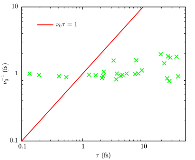
Figure 9: Comparison of the reciprocal of the minimum photon frequency to produce the photoelectric effect and the mean time between collisions for various metals. From left to right, the symbols correspond to Mn, Bi, Hg, Sb, Pb, Ga, Fe, Sn, Tl, Ba, Be, In, Nb, Zn, Cd, Al, Sr, Li, Mg, Cs, Ca, Cu, Rb, Au, Na, K, and Ag. The region well above the line of $\nu_{0}\tau=1$ is disfavored by the photoelectric effect.

4.4 A Wavy View

In retrospect, the which-way question becomes irrelevant if the photon is a pure wave.

Let us examine the experiment in this work with a wave interpretation. The photon wave is described by its shape, momentum, and time evolution. When there is no lens between the camera and the slits, one gets an image of randomly sampled wave shape. With sufficient sampling, the fringes appear, but the momentum information, which would tell the path of the photon in the particle interpretation, is lost. An ideal lens without the aperture stop would Fourier transform the photon wave to provide a momentum representation in the image plane. The shape information is still encoded in the Fourier phases, which, unfortunately, is discarded by the camera. As such, one cannot manipulate a single image of the two slits in any way to recover the illumination pattern at the pupil. The effect of the aperture stop is a convolution of its Fourier modes with the illumination pattern’s Fourier modes. The scan shifts the relative phases between the two parties in the convolution. After taking the data of many shifts, one recovers shape information to satisfaction. Fig. 8 is quite interesting. It shows that the two momentum components of the photon wave have very similar (perhaps the same) shapes, analogous to self-interference occurring regardless which slit a particle photon goes through.

How about other particles? The same arguments should apply. If one agrees that neither localized events nor quantized energies constitute a necessary condition for declaring detection of particles rather than waves, then there is little evidence or need for “particles” to be particles. I therefore propose to describe quantum objects in a wave-only representation. Consequently, the concepts of interference and diffraction are not needed anymore, because they can be described by waves passing openings of different sorts. Another benefit is that we do not have to impose Heisenberg’s uncertainty principle on particles if they do not exist. One can prove the uncertainty principle mathematically for wave functions, but not particles with bare particle properties.

So, are we waves after all?

Epilogue

Although the particle picture of light has difficulty in explaining Young’s double-slit experiment, it is so well shielded by complementarity that an explanation has long been deemed unnecessary. After all, the wave picture of light is not without its own problem. This work tries to lift the shield and makes an attempt to reconcile the wave picture and energy quanta heuristically, though I think quantum electrodynamics has already provided a formal solution. It is certainly premature to discard the concept of particles at this point, but the need for a full understanding of particle-wave duality is nonetheless outstanding.

References

- [1] W. K. Wootters and W. H. Zurek, Phys. Rev. D 19, 473 (January 1979).
- [2] L. S. Bartell, Phys. Rev. D 21, 1698 (March 1980).
- [3] P. Mittelstaedt, A. Prieur and R. Schieder, Found. Phys. 17, 891 (September 1987).
- [4] D. M. Greenberger and A. Yasin, Phys. Lett. A 128, 391 (April 1988).
- [5] G. Jaeger, A. Shimony and L. Vaidman, Phys. Rev. A 51, 54 (January 1995).
- [6] B.-G. Englert, Phys. Rev. Lett. 77, 2154 (September 1996).
- [7] S. Kocsis, B. Braverman, S. Ravets, M. J. Stevens, R. P. Mirin, L. K. Shalm and A. M. Steinberg, Science 332, p. 1170 (June 2011).
- [8] R. Menzel, D. Puhlmann, A. Heuer and W. P. Schleich, Proc. Nat. Acad. Sci. 109, 9314 (2012).
- [9] S. S. Afshar, Violation of the principle of complementarity, and its implications, in The Nature of Light: What Is a Photon?, eds. C. Roychoudhuri and K. Creath, Proc. SPIE, Vol. 5866 (SPIE, August 2005).
- [10] N. Bohr, Nature 121, 580 (April 1928).
- [11] A. S. Fruchter and R. N. Hook, Pub. Astron. Soc. Pac. 114, 144 (February 2002).
- [12] W. Cash, Nature 442, 51 (July 2006).
- [13] I. Bialynicki-Birula, Acta Phys. Pol. A 86, p. 97 (September 1994).
- [14] J. E. Sipe, Phys. Rev. A 52, 1875 (September 1995).
- [15] A. Einstein, Annalen der Physik 322, 132 (1905).
- [16] D. Haar, The old quantum theory (Pergamon Press, 1967).
- [17] P. Drude, Annalen der Physik 306, 566 (1900).
- [18] M. Göppert-Mayer, Annalen der Physik 401, 273 (1931).
- [19] W. Kaiser and C. G. Garrett, Phys. Rev. Lett. 7, 229 (September 1961).