The amplitudes and the structure of the charge density wave in YBCO

Abstract

We find unknown $s$- and $d$-wave amplitudes of the recently discovered charge density wave (CDW) in underdoped cuprates. To do so we perform a combined analysis of experimental data for ortho-II YBa₂Cu₃O_y. The analysis includes data on nuclear magnetic resonance, resonant inelastic X-ray scattering, and hard X-ray diffraction. The amplitude of doping modulation found in our analysis is $3.5\cdot 10^{-3}$ in a low magnetic field and $T=60$K, the amplitude is $6.5\cdot 10^{-3}$ in a magnetic field of 30T and $T=1.3$K. The values are in units of elementary charge per unit cell of a CuO₂ plane. We show that the data rule out a checkerboard pattern, and we also show that the data might rule out mechanisms of the CDW which do not include phonons.

The recent discovery of the charge density wave (CDW) in YBCO and other cuprates gave a new twist to physics of high-T_c superconductivity. Existence of a new charge ordered phase has been reported in bulk sensitive nuclear magnetic resonance (NMR) measurements Wu2011 ; Wu2013 ; Wu2015 , resonant inelastic X-ray scattering (RIXS) Ghiringhelli2012 ; Achkar2012 ; Blackburn2013 , resonant X-ray scattering Comin2014 and hard X-ray diffraction (XRD) Chang2012 . Additional non-direct evidence comes from measurements of ultrasound speed LeBeouf2012 and Kerr rotation angle Xia2008 .

While the microscopic mechanism of the CDW and its relation to superconductivity remains an enigma, there are several firmly established facts listed below, here we specifically refer to YBCO. (i) The CDW state arises in the underdoped regime within the doping range $0.08\leq p\leq 0.13$. (ii) The onset temperature of CDW at doping $p\sim 0.1$ is $T_{CDW}\approx 150$ K, which is between the pseudogap temperature $T^{*}$ and the superconducting temperature $T_{c}$, $T_{c}<T_{CDW}<T^{*}$. (iii) The CDW “competes” with superconductivity, the CDW amplitude is suppressed at $T<T_{c}$. Probably due to this reason the CDW amplitude at $T<T_{c}$ is enhanced by a magnetic field that suppresses superconductivity. (iv) The CDW wave-vector is directed along the CuO link in the CuO₂ plane. (v) The wave-vector $Q\approx 0.31$ r.l.u. only very weakly depends on doping. (vi) The CDW is essentially two-dimensional in low magnetic fields, the correlation length in the $c$-direction is about one lattice spacing, while the in-plane correlation length is $\xi_{a,b}\sim 20$ lattice spacings. (vii) In high magnetic fields ($B>15$ T) and low temperatures ($T<50$ K) the CDW exhibits three-dimensional correlations with the correlation length in the $c$-direction $\xi_{c}\sim 5$ lattice spacings Gerber2015 ; Chang2015 . (viii) Ionic displacements in the CDW are about $10^{-3}\AA$ Forgan2015 .

In spite of numerous experimental and theoretical works, there are two major unsolved problems in the phenomenology of the CDW. (i) The amplitude of the electron density modulation remains undetermined. (ii) The intracell spatial charge pattern is unclear, while there are indications from RIXS Comin2015 and from scanning tunneling microscopy Hamidian2015 that the pattern is a combination of $s$- and $d$-waves. The major goal of the present work is to resolve the open problems. We stress that in the present paper we perform combined analysis of experimental data to resolve the problems of the phenomenology, but we do not build a microscopic model of the CDW. While we rely on various data, the most important information in this respect comes from NMR. In particular we use the ortho-II YBCO data. Ortho-II YBCO (doping $p\approx 0.11$) is the least disordered underdoped cuprate and hence it has the narrowest NMR lines. Development of the CDW with decreasing of temperature leads to the broadening of the quadrupole satellites in the NMR spectrum  Wu2011 ; Wu2013 ; Wu2015 . Below we refer the quadrupole satellites as NQR lines. Quite often the term ”NQR” implies zero magnetic field measurements. We stress that it is not true in our case, NQR here means quadrupole satellites of NMR lines. The broadening is directly proportional to the CDW amplitude with the coefficients determined in Ref. Haase2004 . So, one can find the CDW amplitude and this is the idea of the present analysis. Moreover, combining the data on copper and oxygen NMR we deduce the CDW intracell pattern within the CuO₂ plane.

The second goal of the present work is “partially theoretical”. Based on the phonon softening data LeTacon2014 we are able to separate between two broad classes of possible mechanisms responsible for the formation of the CDW. (i) In the first class the CDW is driven purely by strongly correlated electrons which generate the charge wave. In this case phonons and the lattice are only spectators which follow electrons. (ii) In the second class, which we call “the Peierls/Kohn” scenario, both electrons and phonons are involved in the CDW development on equal footing. We argue that the phonon softening data  LeTacon2014 potentially supports the second scenario.

The CDW implies modulation of electron charge density on copper and oxygen sites in the CuO₂-planes. Our notations correspond to the orthorhombic YBCO, the axis c is orthogonal to the CuO₂-plane, the in-plane axes $a$ and $b$ are directed perpendicular and parallel to the oxygen chains, respectively. Usually the CDW is described in terms of $s$-, $s^{\prime}$-, and $d$-wave components with amplitudes $A_{s}$, $A_{s^{\prime}}$, and $A_{d}$, see e.g. Refs. Comin2015 ; Fujita2014 ; Hamidian2015 . The $s$-wave component corresponds to the modulation of the population of Cu $3d_{x^{2}-y^{2}}$ orbitals, and $s^{\prime}$- and $d$-wave components correspond to the modulation of the populations of oxygen $2p_{\sigma}$ orbitals:

$$\delta n_{d}=A_{s}\cos[{\bm{Q}}\cdot{\bm{r}}+\phi_{s}],$$ (1)

$$\delta n_{px}=A_{s^{\prime}}\cos[{\bm{Q}}\cdot{\bm{r}}+\phi_{s^{\prime}}]+A_{d}\cos[{\bm{Q}}\cdot{\bm{r}}+\phi_{d}],$$

$$\delta n_{py}=A_{s^{\prime}}\cos[{\bm{Q}}\cdot{\bm{r}}+\phi_{s^{\prime}}]-A_{d}\cos[{\bm{Q}}\cdot{\bm{r}}+\phi_{d}].$$

Here $\bm{Q}$ is the wave vector of the CDW, directed along $a$ or $b$ crystal axis [${\bm{Q}}=(Q,0)$ or ${\bm{Q}}=(0,Q)$] and $\phi_{s}$, $\phi_{s^{\prime}}$, $\phi_{d}$ are the phases of $s$-, $s^{\prime}$- and $d$-waves. The subscripts “$x$” and “$y$” in Eq. (1) indicate different oxygen sites within the CuO₂-plane unit cell. The standard nomenclature of the oxygen sites in YBCO is O(2) and O(3). The O(2) 2p_σ-orbital is parallel to the axis “$a$”, and the O(3) 2p_σ-orbital is parallel to the axis “$b$”, see Fig. 1. For the CDW wave-vector $\bm{Q}$ directed along the $a$-axis, the “$x$”-site is O(2) and the “$y$”-site is O(3) as shown in Fig. 1. In the same figure we indicate excess charge corresponding to $s$, $s^{\prime}$-, and $d$-waves. For ${\bm{Q}}$ orientated along the axis “$b$” the “$x$”-site is O(3), and the “$y$”-site is O(2).

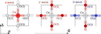
Figure 1: Intra-unit cell patterns of the CDW directed along the a-axis, ${\bm{Q}}=(Q,0)$: $s$-wave, $s^{\prime}$-wave, and $d$-wave. Positive and negative excess charge variations are shown in red and blue respectively.

According to the analysis Haase2004 the NQR frequency of a particular ¹⁷O nucleus is proportional to the local hole density $n_{p}$ at this site, and of course it depends on the orientation of the magnetic field with respect to the oxygen p-orbital,

$$B\perp 2p_{\sigma}:\ f_{O\perp}\approx 1.23MHz\times n_{p}+C_{1},$$

$$B\ ||\ 2p_{\sigma}:\ f_{O||}\approx 2.45MHz\times n_{p}+C_{2},$$ (2)

where $B$ is the external magnetic field of NMR. Constants $C_{1}$ and $C_{2}$ are due to other ions in the lattice; generally they depend on the position of the oxygen ion in the lattice. Typical values of these constants are: $C_{1}\sim 0.2$ MHz, $C_{2}\sim 0.5$ MHz. According to the same analysis  Haase2004 the ⁶³Cu NQR frequency is proportional to the local hole density $n_{d}$ at the Cu site and also $n_{p}$ at the adjacent oxygen sites,

$$\text{Cu}^{63}(B\,||\,{c}):\ f \approx 94.3MHz\times n_{d}$$

$$- 11MHz\times[4-(n_{pa}+n_{pb})]+C_{3}.$$

Here the “ion-related” constant $C_{3}\sim-6$ MHz.

There are two mechanisms for the position dependent variation of the NQR frequency which are related to the CDW, (i) a variation of the local densities $n_{d},n_{p}$, (ii) a variation of the ions’ positions. The position dependent frequency variation leads to the observed inhomogeneous broadening of the NQR line. Let us show that the mechanism (ii) is negligible. Only in-plane displacements of ions contribute to (ii) in the first order in the ion displacement. The magnitudes of the relative in-plane displacements of Cu and O ions are $\delta r/r\lesssim 10^{-3}$ Forgan2015 , where $r\approx 2\AA$ is the Cu-O distance. Hence we can expect a lattice-related variation of e.g. oxygen $f_{\perp}$ at the level $\delta f_{\perp}\sim C_{1}\delta r/r\sim 0.2$ kHz. This is two orders of magnitude smaller than the CDW related broadening $\sim 10$ kHz observed experimentally. For copper nuclei the expected ion-related broadening comes mainly from the $11\times 4$MHz term in  (The amplitudes and the structure of the charge density wave in YBCO), $\delta f\sim\delta r/r\times 44\text{ MHz }\sim 0.04$ MHz. Again, this is much smaller than the observed broadening $\sim 1$ MHz. These estimates demonstrate that one can neglect the contribution of the lattice distortion in the NQR broadening. Therefore, below we consider only the broadening mechanism (i) related to variation of hole densities.

Any compound has an intrinsic quenched disorder. The disorder is responsible for the NQR line widths at $T>T_{CDW}$.

The experimental NQR lines in a “weak magnetic field”, $B=12-15$T, are practically symmetric, the analysis of the NQR lines and the corresponding values of full widths at half maximum (FWHM) are presented in Refs. Wu2013 ; Wu2015 . However, the experimental NQR lines in a “strong magnetic field” Wu2011 , $B\approx 30$T, are somewhat asymmetric due to various reasons. The asymmetry brings a small additional uncertainty in the analysis. The “strong field” data is less detailed than the “weak field” data and therefore the additional uncertainty is completely negligible, the “strong field” NQR widths are given in Ref. Wu2011 . Hereafter we assume simple Gaussian lines, $I(f)\propto\exp[-(f-f_{0})^{2}/2\sigma_{0}^{2}]$, where $f_{0}$ is the center of the NQR line, $\sigma_{0}$ corresponds to the intrinsic disorder-related width. At $T<T_{CDW}$ the line shape is changed to

$$I(f)\propto\left\langle\exp\left\{-\frac{[f-f_{0}-\delta f({\bf r})]^{2}}{2\sigma_{0}^{2}}\right\}\right\rangle\ ,$$ (4)

where $\delta f({\bm{r}})$,

$$\delta f({\bm{r}})=A\cos[({\bm{Q}}\cdot{\bm{r}})+\phi]\$$ (5)

follows from Eqs. (The amplitudes and the structure of the charge density wave in YBCO), (The amplitudes and the structure of the charge density wave in YBCO), (1). In particular, in MHz

$$\delta f_{O\perp}=1.23\left\{A_{s^{\prime}}\cos[{\bm{Q}}\cdot{\bm{r}}+\phi_{s^{\prime}}]\pm A_{d}\cos[{\bm{Q}}\cdot{\bm{r}}+\phi_{d}]\right\},$$

$$\delta f_{O||}=2.45\left\{A_{s^{\prime}}\cos[{\bm{Q}}\cdot{\bm{r}}+\phi_{s^{\prime}}]\pm A_{d}\cos[{\bm{Q}}\cdot{\bm{r}}+\phi_{d}]\right\},$$

$$\delta f_{Cu}=94.3A_{s}\cos[{\bm{Q}}\cdot{\bm{r}}+\phi_{s}]+22A_{s^{\prime}}\cos[{\bm{Q}}\cdot{\bm{r}}+\phi_{s^{\prime}}].\$$ (6)

The averaging in Eq. (4), $\left\langle....\right\rangle$, is performed over the position ${\bf r}$ of a given ion (Cu or O) in the CuO plane. A simulation of $I(f)$ in Eq. (4) with $\delta f$ from  (5) is straightforward, the results for several values of the ratio $A/\sigma_{0}$ are presented in Fig. 2a.

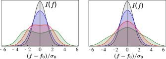
Figure 2: (a) The NQR lineshapes for the stripe-like CDW  (5). (b) The NQR lineshapes for the checkerboard CDW  (7). Both (a) and (b) show the lines for four different values of the CDW amplitude $A$ with respect to the intrinsic broadening, $A/\sigma_{0}=0,1,2,3$.

The CDW leads to the NQR line broadening and at larger amplitudes results in a distinctive double peak structure. For a comparison in the Panel b of Fig. 2 we present the lineshapes obtained with Eq. (4) for the checkerboard density modulation,

$$\delta f({\bm{r}})=\frac{A}{\sqrt{2}}[\cos(Qr_{a})+\cos(Qr_{b})]\ .$$ (7)

Obviously, the lineshapes in panels a and b of Fig. 2 are very different. The checkerboard pattern does not result in the double peak structure even at very large amplitudes. NQR data Wu2011 ; Wu2013 clearly indicate the double peak structure. This is a fingerprint of the stripe-like CDW. Comparison of the experimental NQR lineshapes with Panels b of Fig. 2 rules out the checkerboard scenario at large magnetic field, see also Comin2015stripe ; Fine2016 ; Comin2016 .

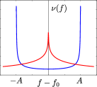
Figure 3: “Density of states” $\nu(f)$ for the stripe CDW (blue line) and for the checkerboard CDW (red line). The two singularities at $f-f_{0}=\pm A$ in the case of the stripe-like CDW result in the double peak structure of the NQR lines.

The qualitative difference between the lineshapes corresponding to the stripe and the checkerboard patterns is a “density of states” effect. Indeed, the NQR intensity (4) can be written in terms of the “density of states”

$$I(f)\propto\left\langle\ldots\right\rangle=\int dS\,(\ldots)=\int df\,\nu(f)(\ldots),$$ (8)

where $(\ldots)$ denotes the Gaussian exponent in (4), $dS$ is the element of area in the CuO₂ plane. The “density of states” $\nu(f)=\int dS\,\delta(f-f_{0}-\delta f(\bm{r}))$ in the case of the stripe-like CDW (5) has two singularities, see Fig. 3, at points $f-f_{0}=\pm A$. The singularities result in two peaks in the NQR spectrum. On the other hand, in the case of the checkerboard CDW (7) the “density of states” $\nu(f)$ has a single maximum at $f=f_{0}$, see Fig. 3, leading to a single-peak NQR lineshape. After averaging over the $(Q,0)$ and $(0,Q)$ stripe domains the double-peak NQR lineshape is intact. Of course this is true only because the size of the domains ($\xi_{a,b}\sim 20-60$ lattice spacings) is much larger then the period of the CDW ($2\pi/Q\approx 3.2$ lattice spacings).

Numerical integration (averaging) in (4) shows that the full NQR line width at half maximum can be approximated as

$$\Gamma_{0}=\sqrt{8\ln 2}\sigma_{0},$$

$$\Gamma\approx\sqrt{\Gamma_{0}^{2}+4\ln 2A^{2}}\ ,\ \ \ \ \ \ \ \text{if}\ \ \Gamma<\Gamma_{0},$$

$$\Gamma\approx 1.2\sqrt{\Gamma_{0}^{2}+4\ln 2A^{2}}\ ,\ \ \ \text{if}\ \ \Gamma>2\Gamma_{0}.$$ (9)

Note that this is the FWHM even for the non-Gaussian line shape like that in Fig. 2a. All the data we use below are in the regime $\Gamma\geq 2\Gamma_{0}$.

The typical dependence of the experimental NQR line width Wu2015 on temperature is sketched in Fig. 4.

Figure 4: A schematic sketch of the temperature dependence of the NQR line width Wu2015 . $\Gamma_{0}$ is the width at the temperature $T_{CDW}$, where the broadening starts to increase with temperature lowering, and $\Gamma_{1}$ is the width at the lowest available temperature.

Hereafter we denote by $\Gamma_{0}$ the value of the width at the temperature, where the width starts to increase with lowering of temperature, and by $\Gamma_{1}$ the value of the width at the lowest available temperature, as indicated in Fig. 4. The increase of the width at low temperatures is due to the CDW development. Comparing the data with Eqs. (The amplitudes and the structure of the charge density wave in YBCO) we can find the CDW amplitudes. There are two distinct Cu positions in ortho-II YBCO, Cu(2E) and Cu(2F), that reside under the empty (E) and full( F) oxygen chains, respectively. There are also three distinct in-plane oxygen positions, O(2), O(3F), and O(3E). The O(2) $2p_{\sigma}$ orbital is oriented along the $a$-axis, and the O(3F), O(3E) $2p_{\sigma}$ orbitals are oriented along the $b$-axis (see Fig. 1). O(3F) resides under the full chain and O(3E) resides under the empty chain. The NQR broadening data for Cu(2E) and Cu(2F) are almost identical, the same is true for O(3F) and O(3E). Therefore, in our analysis we do not distinguish “E” and “F” and refer to them as Cu(2) and O(3) respectively.

It is worth noting that the NQR lines have been measured in NMR experiments. Therefore, the actual line broadening is a combined effect of the NQR broadening and the NMR broadening. The NMR broadening comes from the magnetic Knight shift which is proportional to the charge density modulation. The Knight shift broadening is itself an interesting effect which can bring additional information about CDW. However, our present analysis is aimed at NQR. The structure of NMR satellites enables the subtraction of the Knight shift effect from the data. The subtraction results in the “rectified” NQR line widths, which we use in our analysis. The rectified NQR line widths obtained in Refs. Wu2015 ; Julien for different ions and for different orientations of magnetic field are listed in the second and third columns of Table 1. In this case the magnetic field is $B=12-15$T, $\Gamma_{0}$ corresponds to 150K and $\Gamma_{1}$ corresponds to 60K.

	$\Gamma_{0}(kHz)$	$\Gamma_{1}(kHz)$	$|A_{s}+0.23A_{s^{\prime}}|$
Cu(2),  B$||$c	230(30)	460(80)	2.0(0.5)
			$\sqrt{A_{s^{\prime}}^{2}+A_{d}^{2}}$
O(2), $2p_{\sigma}||a$, B$||$a	6.0(0.5)	16.0(1.3)	2.9(0.3)
O(2), $2p_{\sigma}||a$, B$||$b	6.0(0.6)	15.0(0.8)	5.4(0.4)
O(2), $2p_{\sigma}||a$, B$||$c ${+20^{o}}$	5.0(2.0)	16.0(2.5)	6.0(1.1)
O(3), $2p_{\sigma}||b$, B$||$a	6.0(1.0)	11.0(1.8)	3.6(0.9)
O(3), $2p_{\sigma}||b$, B$||$b	5.0(2.0)	12.0(2.0)	2.1(0.5)
O(3), $2p_{\sigma}||b$, B$||$c +20o	9.0(2.3)	18.0(2.3)	6.1(1.4)

Table 1: NQR data for ortho-II YBCO in magnetic field $B=12-15$T. The line widths, $\Gamma_{0}=\Gamma_{T=150K}$ and $\Gamma_{1}=\Gamma_{T=60K}$, are measured for different ions and for different orientations of the magnetic field Wu2015 ; Julien . The last column displays the CDW amplitudes deduced from the particular line. Figures in brackets represent crude estimates of error bars.

Figures in brackets represent crude estimates of error bars.

The CDW-induced broadening at oxygen sites comes from contributions of the $s^{\prime}$- and $d$-waves, see Eq. (The amplitudes and the structure of the charge density wave in YBCO). RIXS and XRD data Ghiringhelli2012 ; Achkar2012 ; Chang2012 ; Blackburn2013 suggest that the CDW state consists of equally probable domains with the one-dimensional CDW along $(Q,0)$ and $(0,Q)$ directions. This means, that even if the phases of $s^{\prime}$ and $d$-wave are locked in a domain, say $\phi_{s^{\prime}}=\phi_{d}$, the $s^{\prime}$-$d$ interference disappears from the oxygen broadening after averaging over orientations of the domains. Hence, comparing Eqs. (5) and  (The amplitudes and the structure of the charge density wave in YBCO) we conclude that for the oxygen sites $A=K\sqrt{A_{s^{\prime}}^{2}+A_{d}^{2}}$ with the coefficient $K=1.23$MHz or $K=2.45$MHz dependent on the orientation of the magnetic field. Using the experimental widths presented in Table 1 together with Eq. (The amplitudes and the structure of the charge density wave in YBCO) one finds values of $\sqrt{A_{s^{\prime}}^{2}+A_{d}^{2}}$ for each particular oxygen ion and orientation of the magnetic field. The values with indicative error bars are listed in the last column of Table 1. The average over the six different cases presented in the Table is

$$\sqrt{A_{s^{\prime}}^{2}+A_{d}^{2}}=3.8\cdot 10^{-3}\ .$$ (10)

Note, that the indicative error bars in Table 1 are not statistical, therefore in Eq. (10) we present the simple average value.

The CDW-induced broadening at Cu sites comes from contributions of $s$- and $s^{\prime}$-waves, see Eq. (The amplitudes and the structure of the charge density wave in YBCO). Below we assume that the phases are locked, $\phi_{s}=\phi_{s^{\prime}}$. Hence comparing Eqs. (5) and  (The amplitudes and the structure of the charge density wave in YBCO) we conclude that for Cu sites $A=94.3|A_{s}+0.23A_{s^{\prime}}|$MHz.

Using the experimental widths presented in the top line of Table 1 together with Eq. (The amplitudes and the structure of the charge density wave in YBCO) we find

$$\left|A_{s}+0.23A_{s^{\prime}}\right|=2.0\cdot 10^{-3}\ .$$ (11)

It is very natural to assume that the amplitudes $A_{s}$ and $A_{s^{\prime}}$ are related as components of Zhang-Rice singlet, $A_{s}\approx 2A_{s^{\prime}}$, see Ref. Haase2004 . Hence, using (10), (11) we come to the following CDW amplitudes at $T=60$K and $B\approx 12-15$T,

$$A_{s}=1.8\cdot 10^{-3},\ \ A_{s^{\prime}}=0.87\cdot 10^{-3},$$

$$A_{d}=3.8\cdot 10^{-3},\ \ \delta p=A_{s}+2A_{s^{\prime}}=3.5\cdot 10^{-3}\ .$$ (12)

The values of $A_{s,s^{\prime},d}$ are in units of the number of holes per atomic site, and $\delta p$ is the doping modulation amplitude in units of the number of holes per unit cell of a CuO₂ plane. Values of the amplitudes have not been reported previously, but the ratios have been deduced from the polarization-resolved resonant X-ray scattering Comin2015 . Our ratio $A_{s^{\prime}}/A_{d}\approx 0.23$ is reasonably close to the value $A_{s^{\prime}}/A_{d}\approx 0.27$ obtained in Ref. Comin2015 , however the ratio $A_{s}/A_{d}\approx 0.47$ is significantly larger than the value reported in Ref. Comin2015 .

Superficially our ratio $A_{s^{\prime}}/A_{d}\approx 0.23$ is reasonably close to the value $A_{s^{\prime}}/A_{d}\approx 0.27$ obtained in Ref. Comin2015 , on the other hand the ratio $A_{s}/A_{d}\approx 0.47$ is significantly larger than the value reported in Ref. Comin2015 . However, one has to be careful making a direct comparison of our results with Ref. Comin2015 . The analysis Comin2015 assumes either $s+d$ or $s^{\prime}+d$ models, while we keep the three components ($s+s^{\prime}+d$ model). For example, it is easy to check that the $s^{\prime}+d$ model ($s=0$) is inconsistent with the NQR data, so the agreement in the value $A_{s^{\prime}}/A_{d}\approx 0.27$ is purely accidental. On the other hand, in principle we can fit the NQR data by the $s+d$ model ($s^{\prime}=0$), this results in $A_{s}/A_{d}\approx 0.53$ that is inconsistent with Comin2015 .

The ratios of the CDW amplitudes $A_{s}/A_{d}\sim 0.2$, $A_{s^{\prime}}/A_{d}\sim 0.1$ have been reported in STM measurements with BSCCO and NaCCOC Fujita2014 . Comparing these ratios (although measured in different cuprates) with our results we see that Fujita2014 indicates dominance of the $d$-wave component, whereas in our analysis the $s$-wave amplitude is about a half of the $d$-wave amplitude. We do not have an explanation for the discrepancy between our results and REXS/STM measurements Comin2015 ; Fujita2014 , moreover REXS and STM are inconsistent with each other. The advantage of our analysis is that it is very simple and straightforward and, of course, NQR is a bulk probe.

Unfortunately, NQR data for magnetic field $B\approx 30$T are not that detailed as that for $B\approx 12-15$T. Nevertheless, based on the Cu NQR/NMR line broadening measured in Ref. Wu2011 and rectifying the Cu NQR line width (subtracting the Knight shift), we conclude that $\Gamma_{0}=\Gamma_{T=75K}=0.6$MHz and $\Gamma_{1}=\Gamma_{T=1.3K}=1.0$MHz. Hence, using the same procedure as that for the low magnetic field, we find $\left|A_{s}+0.23A_{s^{\prime}}\right|=3.7\cdot 10^{-3}$. Again, assuming the Zhang-Rice singlet ratio, $A_{s}\approx 2A_{s^{\prime}}$, we find the $s$-wave CDW amplitudes for $B\approx 30$T and $T=1.3$K:

$$A_{s}=3.3\cdot 10^{-3},\ \ A_{s^{\prime}}=1.6\cdot 10^{-3},$$

$$\delta p=A_{s}+2A_{s^{\prime}}=6.5\cdot 10^{-3}\ .$$ (13)

The doping modulation amplitude $\delta p$ is about two times smaller than the estimate presented in Ref. Wu2011 . Unfortunately, data Wu2013 are not sufficient for unambiguous subtraction of the Knight shift broadening from oxygen lines, so the determination of $A_{d}$ is less accurate. However, roughly at $B\approx 30$T and $T=1.3$K the value is $A_{d}\sim 6\cdot 10^{-3}$.

To complete our phenomenological analysis we comment on two broad classes of possible mechanisms of the CDW instability. (i) In the first class the CDW instability is driven purely by strongly correlated electrons which generate the charge wave. It can be due to electron-electron interaction mediated by spin fluctuations and/or due to the Coulomb interaction, see e.g. Refs Volkov2015 ; Wang2014 . We call this class of CDW formation mechanisms the “electronic scenario”. In this scenario phonons/lattice are not crucial for the CDW instability, they are only spectators that follow electrons. (ii) In the second class which we call the “Peierls/Kohn scenario” and which is known in some other compounds Renker ; Johannes2008 ; Hoesch2009 , both electrons and phonons are involved in the CDW development on equal footing. We argue that the phonon softening data might support the second class.

A very significant softening of transverse acoustic and transverse optical modes in YBCO has been observed in Ref. LeTacon2014 . The softening data are reproduced in Fig. 5a. The anomaly is very narrow in momentum space, $\delta q\approx 0.04$ r.l.u., and it is only two times broader than the width of the elastic CDW peak, $\delta q=1/\xi_{a,b}\approx 0.02$ r.l.u. measured in RIXS and XRD Ghiringhelli2012 ; Chang2012 ; Blackburn2013 .

Figure 5: (a): Phonon anomaly (dip) in the dispersion of transverse acoustic (TA) and transverse optical (TO) modes at ${\bf q}=(0,Q,6.5)$ in YBa₂Cu₃O_6.6 LeTacon2014 . (b) The expected phonon dispersion in the “electronic scenario”. Blue solid lines show the dispersion in a perfect long-range CDW, grey lines represent the shadow bands. For a finite CDW correlation length the shadow bands practically disappear and solid blue lines become connected by the red solid line.

Our observation is very simple, in the case of the “electronic” scenario, the electronic CDW creates a weak periodic potential $V=V_{0}\cos({\bf Q}\cdot{\bf r}+\phi)$ for phonons. Diffraction of phonons from the potential must lead to the usual band-structure discontinuity of the phonon dispersion $\omega_{q}$ at $q=Q$ as it is shown by blue lines in Panel b of Fig. 5. In the presence of the finite correlation length of the CDW the discontinuity is healed as it is shown by the red solid line at the same panel, and combined blue-red solid line shows the expected phonon dispersion. In Supplementary material we present a calculation which supports this picture, but generally the picture is very intuitive. Obviously, this physical picture for the phonon dispersion is qualitatively different from the experimental data in Panel a of Fig. 5. On the other hand the “Peierls/Kohn scenario”, where both electrons and phonons are equally involved in the CDW development, leads to phonon dispersions like that in Fig. 5a. This has been observed in several compounds, see e.g. Refs. Renker ; Hoesch2009 . Even though the phenomenological observation does not explain the mechanism of the CDW in underdoped cuprates, the observation poses a significant challenge to theoretical models based on “the electronic scenario” of the CDW formation. Furthermore, the phonon softening is generally expected in the “Kohn/Peierls scenario”, which is likely to be the case in YBCO. At the same time our arguments in favour of the “Kohn/Peierls scenario” are not quite conclusive. Indeed, it seems that the “Kohn/Peierls scenario” does not provide an explanation of the strong broadening of TA and TO phonon modes at $T<T_{CDW}$ [19], as well as it does not explain why the phonon softening appears only in superconducting state $T<T_{c}$. So the last point of our work is less solid than the main results concerning the amplitudes of the CDW. Nevertheless, we believe that the presented discussion of the “Kohn/Peierls scenario” versus “electronic scenario” is useful for future work on the microscopic mechanism of the CDW.

In conclusion, our analysis of available experimental data has resolved open problems in the phenomenology of the charge density wave (CDW) in underdoped cuprates. We have determined the amplitudes of $s$-, $s^{\prime}$-, and $d$-wave components of the density wave. The amplitudes at low magnetic field and temperature $T=60$K are given in Eq. (The amplitudes and the structure of the charge density wave in YBCO), and the amplitudes for magnetic field $B=30$T and temperature $T=1.3$K are given in Eq. (The amplitudes and the structure of the charge density wave in YBCO). We show that the data rule out a checkerboard pattern, and we also argue that the data might rule out mechanisms of the CDW which do not include phonons.

.1 Acknowledgements

We thank M.-H. Julien, M. Le Tacon, J. Haase and A. Damascelli for communications, discussions, and very important comments. The work has been supported by the Australian Research Council, grants DP110102123 and DP160103630.

.2 Author contribution

Both authors, Y. A. K. and O. P. S, contributed to all aspects of this work.

.3 Competing financial interests

The authors declare no competing financial interests.

Appendix A Ginzburg-Landau model of the CDW and phonon dispersion

Here we consider a simple phenomenological Ginzburg-Landau model of the CDW developed in purely electron sector. Phonons weakly interact with electrons and follow the developed CDW as “spectators”. This is the first scenario discussed in the main text. Our analysis below shows that the phonon softening data does not support this scenario.

Let us consider a quasi-one dimensional (stripe-like) CDW, we direct the $x$ axis along the CDW wave-vector. The CDW can be represented as a collective bosonic mode ($\psi$) in the electronic system. The effective Ginzburg-Landau-like Lagrangian for the CDW mode $\psi$ reads

$$\mathcal{L}_{\psi}=\frac{\dot{\psi}^{2}}{2}-\psi\frac{\hat{\Omega}^{2}}{2}\psi-\frac{\alpha}{4}\psi^{4}\ ,$$ (14)

where $\psi(r)$ is a variation of electron density, $\hat{\Omega}^{2}/2$ is operator of “stiffness” of the CDW mode, and $\alpha>0$ is a self-action constant. In momentum representation $\Omega^{2}_{q}$ is a simple function sketched in Fig. 6.

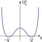
Figure 6: A sketch of the effective kinetic energy $\Omega^{2}_{q}$ of the electronic CDW mode $\psi$.

Kinetic energy has minima at $q_{x}=\pm Q$, and we can represent it as

$$\Omega_{q}^{2}=\Omega_{Q}^{2}+\kappa(q_{x}^{2}-Q^{2})^{2}/4,$$ (15)

where $\kappa$ is a some constant. Importantly the minimal value of $\Omega_{\pm Q}^{2}$ is negative, $\Omega_{\pm Q}^{2}<0,$ providing formation of the incommensurate CDW with the wave vector $Q$. The density variation is real, hence

$$\psi(x)=2|\psi_{Q}|\cos(Qx+\phi),$$ (16)

here $\psi_{Q}$ is a Fourier component of $\psi(r)$. In a perfect system the phase $\phi$ is arbitrary and this must result in a Goldstone sliding mode. Of course a disorder pins the phase. A similar phenomenological approach was successfully applied to describe a CDW state in transition-metal dichalcogenides McMillan1975 .

To find the CDW amplitude one has to minimize the energy

$$E_{\psi}=\int d^{2}r\left(\psi\frac{\hat{\Omega}^{2}}{2}\psi+\frac{\alpha}{4}\psi^{4}\right).$$ (17)

The saddle-point equation for static $\psi(r)$ reads

$$\hat{\Omega}^{2}\psi+\alpha\psi^{3}=0.$$ (18)

Performing Fourier transform in Eqs. (18) and leaving only the dominating Fourier components with $q=\pm Q$ we find

$$|\psi_{Q}|^{2}=-\Omega^{2}_{Q}/3\alpha.$$ (19)

To find the CDW excitation spectrum we expand energy (17) up to second order in fluctuations on the top of the ground state (16),(19),

$$\delta^{2}E_{\psi}=\int d^{2}r\left(\delta\psi\frac{\hat{\Omega}^{2}}{2}\delta\psi+\frac{3\alpha}{2}\psi^{2}(\delta\psi)^{2}\right).$$ (20)

The term $\propto\psi^{2}=|\psi_{Q}|^{2}(2+e^{2i(Qx+\phi)}+e^{-2i(Qx+\phi)})$ in (20) plays role of the effective potential with wave vector $2Q$ for the $\psi$-excitations. This results in a mixing between $\delta\psi_{q}$ and $\delta\psi_{q-2Q}$ (hereafter we assume that $q>0$). Therefore, it is convenient to write the excitation energy as

$$\delta^{2}E_{\psi}=\sum_{q}\Psi_{q}^{\dagger}\begin{pmatrix}\Omega^{2}_{q}+2|\Omega^{2}_{Q}|&|\Omega^{2}_{Q}|e^{2i\phi}\\ |\Omega^{2}_{Q}|e^{-2i\phi}&\Omega^{2}_{q-2Q}+2|\Omega^{2}_{Q}|&\end{pmatrix}\Psi_{q},$$ (21)

where

$$\Psi_{q}=\left(\begin{array}[]{l}\delta\psi_{q}\\ \delta\psi_{q-2Q}\end{array}\right).$$

Euler-Lagrange equation corresponding to (14), (21) results in the two normal modes: the sliding Goldstone mode and the gapped Higgs mode with the energies

$$\epsilon_{Gq}=\sqrt{\kappa Q^{2}}|p_{x}|,$$

$$\epsilon_{Hq}=\sqrt{2|\Omega^{2}_{Q}|+\kappa Q^{2}p_{x}^{2}}$$

$$\bm{p}=\bm{q}-\bm{Q}\ .$$ (22)

The corresponding eigenmodes are

$$\begin{array}[]{c}G_{q}=1/\sqrt{2}(e^{i\phi}\delta\psi_{q}-e^{-i\phi}\delta\psi_{q-2Q}),\\ H_{q}=1/\sqrt{2}(e^{i\phi}\delta\psi_{q}+e^{-i\phi}\delta\psi_{q-2Q}).\end{array}$$ (23)

Interestingly, due to the parabolic behaviour of $\Omega^{2}_{q}$ near $q_{x}=\pm Q$, see Fig. 6, the weights of the states with wave vectors $q$ and $q-2Q$ in (23) are equal in a broad range of momenta around $q=\pm Q$.

The phonon is described by field $\varphi$, the phonon Lagrangian reads

$$\mathcal{L}_{\varphi}=\frac{\dot{\varphi}^{2}}{2}-\varphi\frac{\hat{\omega}^{2}}{2}\varphi,$$ (24)

where $\hat{\omega}^{2}/2$ is the elastic energy of lattice deformation. In momentum representation it is equivalent to the bare phonon dispersion $\omega_{q}$. The CDW and phonons weakly interact, we describe the interaction by the Lagrangian

$$\mathcal{L}_{int}=-\lambda\psi\varphi\ ,$$ (25)

where $\lambda$ is coupling constant. Due to the coupling the CDW creates phonon condensate at $q_{x}=\pm Q$ (static lattice deformation) with amplitude $\varphi_{Q}=-\lambda/\omega^{2}_{Q}\,\psi_{-Q}$. Let us now consider phonon dispersion in the presence of the collective CDW mode. The interaction (25) in combination with Eqs (23) results in the following vertexes describing transition of phonon to the Higgs and Goldstone modes of the CDW.

$$\langle\delta\varphi_{q}|H_{q}\rangle=\langle\delta\varphi_{q}|G_{q}\rangle=\frac{\lambda}{\sqrt{2}}e^{i\phi}$$

$$\langle\delta\varphi_{q-2Q}|H_{q}\rangle=-\langle\delta\varphi_{q-2Q}|G_{q}\rangle=\frac{\lambda}{\sqrt{2}}e^{-i\phi}\ .$$

This leads to normal and anomalous phonon self-energy operators shown in Fig. 7.

Figure 7: Normal and anomalous phonon self-energy

The corresponding analytical expressions are

$$\Sigma^{(n)}_{q}=\frac{\lambda^{2}}{2}\left(\frac{1}{\omega_{q}^{2}-\epsilon_{Hq}^{2}}+\frac{1}{\omega_{q}^{2}-\epsilon_{Gq}^{2}}\right),$$

$$\Sigma_{q}^{(a)}=e^{2i\phi}\Delta_{q}^{2},$$

$$\Delta_{q}^{2}=\frac{\lambda^{2}}{2}\left(\frac{1}{\omega_{q}^{2}-\epsilon_{Hq}^{2}}-\frac{1}{\omega_{q}^{2}-\epsilon_{Gq}^{2}}\right).$$ (26)

A selfenergy generally depends on $q$ and $\omega$. In Eqs.(A) we set $\omega=\omega_{q}$. So ”renormalized” dispersion $\widetilde{\omega}_{q}$ of phonons is described by the eigenvalue problem

$$\widetilde{\omega}_{q}^{2}\Phi_{q}=\begin{pmatrix}\omega_{q}^{2}+\Sigma^{(n)}_{q}&e^{2i\phi}\Delta_{q}^{2}\\ e^{-2i\phi}\Delta_{q}^{2}&\omega_{q-2Q}^{2}+\Sigma^{(n)}_{q-2Q}\end{pmatrix}\Phi_{q}\ ,$$ (27)

where

$$\Phi_{q}=\left(\begin{array}[]{l}\delta\varphi_{q}\\ \delta\varphi_{q-2Q}\end{array}\right).$$ (28)

As it is intuitively clear even without a calculation Eq. (27) is equivalent to scattering of phonon from some effective periodic potential with wave vector $2Q$.

One can represent matrix elements in (27) as

$$\sqrt{\omega_{q}^{2}+\Sigma^{(n)}_{q}}\approx w+cp_{x},$$

$$\sqrt{\omega_{q-2Q}^{2}+\Sigma^{(n)}_{q-2Q}}\approx w-cp_{x},$$

$$\Delta_{q}\approx\Delta\ ,$$ (29)

when the detuning $\bm{p}=\bm{q}-\bm{Q}$ is small. The speed $c$ follows from the overall slope of the phonon dispersion. For the TO mode $w\approx 15$ meV, $c\approx 30$ meV/r.l.u., see Fig. 5a in the main text. The phonon dispersion which follows from (27) and (A),

$$\widetilde{\omega}_{q}^{2}\approx w^{2}\pm\sqrt{4w^{2}c^{2}p_{x}^{2}+\Delta^{4}}\ ,$$ (30)

is shown in Fig.5b in the main text by the blue solid line. Shadow bands are indicated by fading grey lines. Expected intensity of the shadow bands is extremely small. Intensities of the bright (br) and shadow (sh) modes are

$$I_{br}\propto|\delta\varphi_{q}|^{2}=\frac{1}{2}\left(1+\frac{2wcp_{x}}{\sqrt{4w^{2}c^{2}p_{x}^{2}+\Delta^{2}}}\right),$$

$$I_{sh}\propto|\delta\varphi_{q-2Q}|^{2}=\frac{1}{2}\left(1-\frac{2wcp_{x}}{\sqrt{4w^{2}c^{2}p_{x}^{2}+\Delta^{2}}}\right).$$

If the gap in the phonon spectrum ($gap\approx\Delta^{2}/w$) is 3 meV (TO mode), the intensity of the shadow mode practically diminishes at detuning $p_{x}=q_{x}-Q\geq 0.04$ r.l.u.

So far we disregarded temperature and intrinsic disorder. We remind the following experimental observations: (i) the CDW onset temperature is $T_{CDW}\sim 150$K, (ii) the CDW in low/zero magnetic fields is essentially two-dimensional, the correlation length in the $c$-direction is about one lattice spacing while the in-plane correlation length is $\xi_{a,b}\sim 20$ lattice spacings. In agreement with Mermin-Wagner theorem the observation (ii) implies that onset of the CDW at $T=T_{CDW}$ is not a true phase transition, it is a two-dimensional freezing crossover. Hence at $T>T_{CDW}$ the phase $\phi$ fluctuates with time and as a result the off-diagonal matrix element in Eq. (27) is averaged to zero, $e^{2i\phi}\Delta_{q}^{2}\to 0$. Hence the phonon dispersion at $T>T_{CDW}$ near $q_{x}=+Q$ is

$$\widetilde{\omega}_{q}=\sqrt{\omega_{q}^{2}+\Sigma^{(n)}_{q}}\approx w+cp_{x}\ .$$ (31)

At $T<T_{CDW}$ the temporal fluctuations freeze, however due to the quenched disorder the phase $\phi(r)$ is a fluctuating function of coordinate $r$ with the correlation length $\xi_{a,b}$. If $|p_{x}|>1/\xi_{a,b}=0.02$ r.l.u. the spatial fluctuations are not relevant and the phonon dispersion is given by Eq.(30). However, if the detuning is small, $|p_{x}|\ll 1/\xi_{a,b}$, one must average over spatial fluctuations of the phase $\phi$ effectively vanishing the off-diagonal matrix element, $e^{2i\phi}\Delta_{q}^{2}\to 0$. This results in the red solid line connecting the blue solid lines in Fig. 5b in the main text.

All in all the phonon dispersion expected if the “electronic” scenario is realized is shown in Fig. 5b (main text). Obviously, the dispersion is inconsistent with the data. Therefore, we rule out the “electronic” scenario.

References

- (1) Wu, T. et al. Magnetic-field-induced charge-stripe order in the high temperature superconductor YBa2Cu3Oy. Nature 477, 191–194 (2011).
- (2) Wu, T. et al. Emergence of charge order from the vortex state of a high temperature superconductor. Nat. Commun. 4, 2113 (2013).
- (3) Wu, T. et al. Incipient charge order observed by NMR in the normal state of YBa2Cu3Oy. Nat. Commun. 6, 6438 (2015).
- (4) Ghiringhelli, G. et al. Long-range incommensurate charge fluctuations in (Y,Nd)Ba2Cu3O6+x. Science 337, 821–825 (2012).
- (5) Achkar, A. J. et al. Distinct charge orders in the planes and chains of ortho-III ordered YBa2Cu3O6+δ identified by resonant elastic X-ray scattering. Phys. Rev. Lett. 109, 167001 (2012).
- (6) Blackburn, E. et al. X-ray diffraction observations of a charge-density-wave order in superconducting ortho-II YBa2Cu3O6.54 single crystals in zero magnetic field. Phys. Rev. Lett. 110, 137004 (2013).
- (7) Comin R. et al. Charge Order Driven by Fermi-Arc Instability in Bi2Sr2-xLaxCuO6+δ. Science 343, 390 (2014).
- (8) Chang, J. et al. Direct observation of competition between superconductivity and charge density wave order in YBa2Cu3O6.67. Nat. Phys. 8, 871–876 (2012).
- (9) Tabis, W. et al. Charge order and its connection with Fermi-liquid charge transport in a pristine high-T c cuprate. Nat. Commun. 5, 5875 (2014).
- (10) LeBeouf, D. et al. Thermodynamic phase diagram of static charge order in underdoped YBa2Cu3Oy. Nat. Phys. 9, 79–83 (2013).
- (11) Xia, J. et al. Polar Kerr-effect measurements of the high-temperature YBa2Cu3O6+x superconductor, evidence for broken symmetry near the pseudogap temperature. Phys. Rev. Lett. 100, 127002 (2008).
- (12) Gerber, S. et al. Three-Dimensional Charge Density Wave Order in YBa2Cu3O6.67 at High Magnetic Fields. Science 350, 949–952 (2015).
- (13) Chang, J. et al. Magnetic field controlled charge density wave coupling in underdoped YBa2Cu3O6+x. Preprint at http://arxiv.org/abs/1511.06092 (2015).
- (14) Forgan, E. M. et al. The microscopic structure of charge density waves in underdoped YBa2Cu3O6.54 revealed by X-ray diffraction. Nat. Comm. 6, 10064 (2015).
- (15) Comin, R. et al. Symmetry of charge order in cuprates. Nat. Mater. 14, 796–800 (2015).
- (16) Fujita, K. et al. Direct phase-sensitive identification of a d-form factor density wave in underdoped cuprates. PNAS 111, E3026-E3032 (2014).
- (17) Hamidian, M. H. et al. Atomic-scale electronic structure of the cuprate -symmetry form factor density wave state. Nat. Phys. 12, 150-156 (2015).
- (18) Haase, J., Sushkov, O. P., Horsch, P. & Williams, G. V. M., Planar Cu and O hole densities in high-Tc cuprates determined with NMR. Phys. Rev. B 69, 094504 (2004).
- (19) Le Tacon, M. et al. Inelastic X-ray scattering in YBa2Cu3O6.6 reveals giant phonon anomalies and elastic central peak due to charge-density-wave formation. Nat. Phys. 10, 52–58 (2014).
- (20) Julien, M.-H., Data for ortho-II YBCO in magnetic field T, private communication.
- (21) Comin, R. et al., Broken translational and rotational symmetry via charge stripe order in underdoped YBa2Cu3O6+y, Science 347, 1335–1339 (2015).
- (22) Fine, B. V. Comment on “Broken translational and rotational symmetry via charge stripe order in underdoped YBa2Cu3O6+y”, Science 351, 235 (2016).
- (23) Comin, R. et al.. Response to Comment on “Broken translational and rotational symmetry via charge stripe order in underdoped YBa2Cu3O6+y”, Science 351, 236 (2016).
- (24) Wang, Y. & Chubukov, A. Charge-density-wave order with momentum (2Q,0) and (0,2Q) within the spin-fermion model: Continuous and discrete symmetry breaking, preemptive composite order, and relation to pseudogap in hole- doped cuprates. Phys. Rev. B 90, 035149 (2014).
- (25) Volkov, P. A. & Efetov, K. B., Spin-fermion model with overlapping hot spots and charge modulation in cuprates. Preprint at http://arxiv.org/abs/1511.01504v1 (2015).
- (26) B. Renker, et al.. Observation of Giant Kohn Anomaly in the One-Dimensional Conductor K2Pt(CN)4Br0.3·3H2O Phys. Rev. Lett., 30, 1144 (1973).
- (27) Johannes, M. & Mazin, I., Fermi surface nesting and the origin of charge density waves in metals. Phys. Rev. B 77, 165135 (2008).
- (28) Hoesch, M. et al. Giant Kohn Anomaly and the Phase Transition in Charge Density Wave ZrTe3. Phys. Rev. Lett. 102, 086402 (2009).

References

- (1) McMillan, W. L., Landau theory of charge-density waves in transition-metal dichalcogenides, Phys. Rev. B 12, 1187-1196 (1975).