Abstract

We describe the algorithms used in the Matlab continuation and bifurcation package pde2path for Hopf bifurcation and continuation of branches of periodic orbits in systems of PDEs in 1, 2, and 3 spatial dimensions, including the computation of Floquet multipliers. We first test the methods on three reaction diffusion examples, namely a complex Ginzburg–Landau equation as a toy problem, a reaction diffusion system on a disk with rotational waves including stable (anti) spirals bifurcating out of the trivial solution, and a Brusselator system with interaction of Turing and Turing–Hopf bifurcations. Then we consider a system from distributed optimal control, which is ill-posed as an initial value problem and thus needs a particularly stable method for computing Floquet multipliers, for which we use a periodic Schur decomposition. The implementation details how to use pde2path on these problems are given in an accompanying tutorial, which, together with all other downloads (function libraries, demos and further documentation) can be found at www.staff.uni-oldenburg.de/hannes.uecker/pde2path.

MSC: 35J47, 35B22, 37M20
Keywords: Hopf bifurcation, periodic orbit continuation, Floquet multipliers, partial differential equations, finite element method, reaction–diffusion, distributed optimal control

1 Introduction

The package pde2path [UWR14, DRUW14, Uec17c] has originally been developed as a continuation/bifurcation package for stationary problems of the form

$$G(u,\lambda):=-\nabla\cdot(c\otimes\nabla u)+au-b\otimes\nabla u-f=0.$$ (1)

Here $u=u(x)\in{\mathbb{R}}^{N}$, $x\in\Omega$ with $\Omega\subset{\mathbb{R}}^{d}$ some bounded domain, $d=1,2,3$, $\lambda\in{\mathbb{R}}^{p}$ is a parameter (vector), and $c\in{\mathbb{R}}^{N\times N\times 2\times 2}$, $b\in{\mathbb{R}}^{N\times N\times 2}$, $a\in{\mathbb{R}}^{N\times N}$ and $f\in{\mathbb{R}}^{N}$ can depend on $x,u,\nabla u$, and parameters. The boundary conditions (BC) are of “generalized Neumann” form, i.e.,

$${\bf n}\cdot(c\otimes\nabla u)+qu=g,$$ (2)

where ${\bf n}$ is the outer normal and again $q\in{\mathbb{R}}^{N\times N}$ and $g\in{\mathbb{R}}^{N}$ may depend on $x$, $u$, $\nabla u$ and parameters. These BC include zero flux BC, and a “stiff spring” approximation of Dirichlet BC via large prefactors in $q$ and $g$, and periodic BC are also supported over suitable domains. Moreover, there are interfaces to couple (1) with additional equations, such as mass conservation, or phase conditions for considering co-moving frames, and to set up extended systems, for instance for fold point and branch point continuation.

pde2path has been applied to various research problems, e.g., patterns in 2D reaction diffusion systems [UW14, Küh15b, Küh15a, SDE⁺15, Wet16, ZUFM17], some problems in fluid dynamics and nonlinear optics [ZHKR15, DU16, EWGT17] and in optimal control [Uec16, GU17]. Here we report on features and algorithms in pde2path to treat Hopf (or Poincaré–Andronov–Hopf) bifurcations and the continuation of time–periodic orbits for systems of the form

$${\partial}_{t}u=-G(u,\lambda),\quad u=u(x,t),\ x\in\Omega\subset{\mathbb{R}}^{d},\ d=1,2,3,\ t\in{\mathbb{R}}\ \ \text{ ($d+1$ dimensional problem),}$$ (3)

with $G$ from (1) and BC from (2). Adding the time dimension makes computations more expensive, such that here we focus on 1D and 2D, and only give one 3D example to illustrate that all user interfaces are essentially dimension independent.

For general introductions to and reviews of (numerical) continuation and bifurcation we recommend [Gov00, Kuz04, Doe07, Sey10], and [Mei00], which has a focus on reaction–diffusion systems. The treatment of large scale problems, typically from the spatial discretization of PDEs, including the continuation of time periodic orbits, has for instance been discussed in [LRSC98, TB00, LR00], and has recently been reviewed in [DWC⁺14]. There, the focus has been on matrix–free methods where the periodic orbits are computed by a shooting method, which can conveniently be implemented if a time–stepper for the given problem is available. In many cases, shooting methods can also be used to investigate the bifurcations from periodic orbits, and to trace bifurcation curves in parameter space, by computing the Floquet multipliers of the periodic orbits. In this direction, see in particular [BT10, SGN13, WIJ13, NS15] for impressive results in fluid problems.

Here we proceed by a collocation (in time) method for the continuation of periodic orbits. With respect to computation time and in particular memory requirements such methods are often more demanding than (matrix free) shooting methods. However, one reason for the efficiency of shooting methods in the works cited above is that there the problems considered are strongly dissipative, with only few eigenvalues of the linearized evolution near the imaginary axis. We also treat such problems, and show that up to moderately large scale they can efficiently be treated by collocation methods as well. However, another class of problems we deal with are canonical systems obtained from distributed optimal control problems with infinite time horizons. Such problems are ill-posed as initial value problems, which seems quite problematic for genuine shooting methods.

We also compute the Floquet multipliers for periodic orbits. For this, a direct approach is to explicitly construct the monodromy matrix from the Jacobian used in the collocation solver for the periodic orbit. We find that this works well for dissipative problems, but completely fails for the ill–posed optimal control problems, and thus we also provide a method based on a periodic Schur decomposition, which can handle this situation. Currently, our Floquet computations can be used to assess the stability of periodic orbits, and for detection of possible bifurcations from them. However, we do not (yet) provide tools for localization of, or branch switching at, such bifurcation points, which is work in progress.

To illustrate the performance of our hopf library we consider four example problems, with the Matlab files included as demo directories in the package download at [Uec17c], where also a pde2path user-guide with installation instruction, a tutorial on Hopf bifurcations with implementation details, and various other tutorials on how to run pde2path are available. The first example is a cubic–quintic complex Ginzburg–Landau (cGL) equation, which we consider over 1D, 2D, and 3D cuboids with homogeneous Neumann and Dirichlet BC, such that we can explicitly calculate all Hopf bifurcation points (HBP) from the trivial branch. For periodic BC we also have the Hopf branches explicitly, which altogether makes the cGL equation a nice toy problem to validate and benchmark our routines. Next we consider a reaction diffusion system from [GKS00] on a circular domain and with somewhat non-standard Robin BC, which lead to rotating waves, and in particular to the bifurcation of (anti) spiral waves out of the trivial solution. Our third example is a Brusselator system from [YDZE02], which shows interesting interactions between Turing branches and Turing–Hopf branches. As a non–dissipative example we treat the canonical system for a simple control problem of “optimal pollution”. This is still of the form (3), but is ill–posed as an initial value problem, since it includes “backward diffusion”. Nevertheless, we continue steady states, and obtain Hopf bifurcations and branches of periodic orbits.

Many of the numerical results on periodic orbits in PDE in the literature, again see [DWC⁺14] for a review, are based on custom made codes, which sometimes do not seem easy to access and modify for non–expert users. Although in some of our research applications we consider problems with on the order of $10^{5}$ unknowns in space, pde2path is not primarily intended for very large scale problems. Instead, the goal of pde2path is to provide a general and easy to use (and modify and extend) toolbox to investigate bifurcations in PDEs of the (rather large) class given by (3). With the hopf library we provide some basic functionality for Hopf bifurcations and continuation of periodic orbits for such PDEs over 1D, 2D, and 3D domains, where at least the 1D cases and simple 2D cases are sufficiently fast to use pde2path as a quick (i.e., interactive) tool for studying interesting problems. The user interfaces reuse the standard pde2path setup, and no new user functions are necessary. Due to higher computational costs in 2+1D, in 3D, or even 3+1D, compared to the 2D case from [UWR14], in the applications given here and the associated tutorials we work with quite coarse meshes, but give a number of comments on how to adaptively generate and work with finer meshes.

In §2 we review some basics of the Hopf bifurcation, of periodic orbit continuation and multiplier computations, and explain their numerical treatment in pde2path. In §3 we present the examples, and §4 contains a brief summary and outlook. The pde2path setup, data structures and help system are reviewed in [dWDR⁺17], and implementation details for the Hopf demos are given in [Uec17a]. For comments, questions, and bugs, please mail to hannes.uecker@uni-oldenburg.de.

Acknowledgment. Many thanks to Francesca Mazzia for providing TOM [MT04], which was essential help for setting up the hopf library; to Uwe Prüfert for providing OOPDE; to Tomas Dohnal, Jens Rademacher and Daniel Wetzel for some testing of the Hopf examples; to Daniel Kressner for pqzschur; to Arnd Scheel for helpful comments on the system in §3.2; and to Dieter Grass for the cooperation on distributed optimal control problems, which was one of my main motivations to implement the hopf library.

2 Hopf bifurcation and periodic orbit continuation in pde2path

Our description of the algorithms is based on the spatial FEM discretization of (3), which, with a slight abuse of notation, we write as

$$M\dot{u}(t)=-G(u(t),\lambda),$$ (4)

where $M\in{\mathbb{R}}^{n_{u}\times n_{u}}$ is the mass matrix, $n_{u}=Nn_{p}$ is the number of unknowns (degrees of freedom DoF) with $n_{p}$ is the number of mesh-points, and, for each $t$,

$$u(t)=(u_{1,1},\ldots,u_{1,n_{p}},u_{2,1},\ldots,u_{N,1},\ldots u_{N,n_{p}})(t)\in{\mathbb{R}}^{n_{u}},$$

and similarly $G:{\mathbb{R}}^{n_{u}}\times{\mathbb{R}}^{p}\rightarrow{\mathbb{R}}^{n_{u}}$. We use the generic name $\lambda$ for the parameter vector, and the active continuation parameter, again see [DRUW14] for details. When in the following we discuss eigenvalues $\mu$ and eigenvectors $\phi$ of the linearization

$$M\dot{v}=-{\partial}_{u}G(u,\lambda)v$$ (5)

of (4) around some (stationary) solution of (4), or simply eigenvalues of ${\partial}_{u}G={\partial}_{u}G(u,\lambda)$, we always mean the generalized eigenvalue problem

$$\mu M\phi={\partial}_{u}G\phi.$$ (6)

Thus eigenvalues of ${\partial}_{u}G$ with negative real parts give dynamical instability of $u$.

Remark 2.1.

For, e.g., the continuation of traveling waves in translationally invariant problems, the PDE (3) is typically transformed to a moving frame $\xi=x-\gamma(t)$, with BC that respect the translational invariance, and where $\dot{\gamma}$ is an unknown wave speed, which yields an additional term $\dot{\gamma}{\partial}_{x}u$ on the rhs of (3). The reliable continuation of traveling then also requires a phase condition, i.e., an additional equation, for instance of the form $q(u)=\left\langle{\partial}_{x}\tilde{u},u\right\rangle\stackrel{{\scriptstyle!}}{{=}}0$, where $\tilde{u}$ is a reference wave (e.g. $\tilde{u}=u_{{\rm old}}$, where $u_{{\rm old}}$ is from a previous continuation step), and $\left\langle u,v\right\rangle=\int_{\Omega}uv\,{\rm d}x$. Together we obtain a differential–algebraic system instead of (4), and similarly for other constraints such as mass conservation, see [DRUW14, §2.4,§2.5] for examples, and for instance [BT07, RU17] for equations with continuous symmetries and the associated “freezing method”. Hopf bifurcations can occur in such systems, see e.g. the Hopf bifurcations from traveling ($\dot{\gamma}\neq 0$) or standing ($\dot{\gamma}=0$) fronts and pulses in [HM94, GAP06, BT07, GF13], but are somewhat more difficult to treat numerically than the case without constraints. Thus, here we restrict to problems of the form (3) without constraints, and hence to (4) on the spatially discretized level, and refer to [RU17, Uec17b] for examples of Hopf bifurcations with constraints in pde2path. For instance, in [RU17, §4] we consider Hopf bifurcations to modulated traveling waves in a model for autocatalysis, and the Hopf bifurcation of standing breathers in a FitzHugh–Nagumo system, and in [Uec17b, §5] the Hopf bifurcation of modulated standing and traveling waves in the Kuramoto-Sivashinky equation with periodic boundary conditions. $\rfloor$

2.1 Branch and Hopf point detection and localization

Hopf bifurcation means the bifurcation of a branch of time periodic orbits from a branch $\lambda\mapsto u(\cdot,\lambda)$ of stationary solutions of (3), or numerically (4). This generically occurs if at some $\lambda=\lambda_{H}$ a pair of simple complex conjugate eigenvalues $\mu_{j}(\lambda)={\overline{\mu}}_{j+1}(\lambda)$ of $G_{u}={\partial}_{u}G(u,\lambda)$ crosses the imaginary axis with nonzero imaginary part and nonzero speed, i.e.,

$$\mu_{j}(\lambda_{H})={\overline{\mu}}_{j}(\lambda_{H})={\rm i}\omega\neq 0,\quad\text{ and }{\rm Re}\mu_{j}^{\prime}(\lambda_{H})\neq 0.$$ (7)

Thus, the first issue is to define a suitable test function $\psi_{H}$ to numerically detect (7). Additionally, we also want to detect real eigenvalues crossing the imaginary axis, i.e.,

$$\mu_{j}(\lambda_{\text{BP}})=0,\quad\text{ and }{\rm Re}\mu_{j}^{\prime}(\lambda_{\text{BP}})\neq 0.$$ (8)

A fast and simple method for (8) is to monitor sign changes of the product

$$\psi(\lambda)=\prod_{i=1,\ldots,n_{u}}\mu_{i}(\lambda)=\det(G_{u})$$ (9)

of all eigenvalues, which even for large $n_{u}$ can be done quickly via the $LU$ factorization of $G_{u}$, respectively the extended matrix in arclength continuation, see [UWR14, §2.1]. This so far has been the standard setting in pde2path, but the drawback of (9) is that the sign of $\psi$ only changes if an odd number of real eigenvalues crosses $0$.

Unfortunately, there is no general method for (7) which can be used for large $n_{u}$. For small systems, one option would be

$$\psi_{H}(\lambda)=\prod_{i}(\mu_{i}(\lambda)+\mu_{i+1}(\lambda)),$$ (10)

where we assume the eigenvalues to be sorted by their real parts. However, this, unlike (9) requires the actual computation of all eigenvalues, which is not feasible for large $n_{u}$. Another option are dyadic products, [Kuz04, Chapter 10], which again is not feasible for large $n_{u}$.

If, on the other hand, (3) is a dissipative problem, then we may try to just compute $n_{\text{eig}}$ eigenvalues of $G_{u}$ of smallest modulus, which, for moderate $n_{\text{eig}}$ can be done efficiently, and to count the number of these eigenvalues which are in the left complex half plane, and from this detect both (7) and (8). The main issue then is to choose $n_{\text{eig}}$, which unfortunately is highly problem dependent, and for a given problem may need to be chosen large again.

The method presented in [GS96] uses complex analysis, namely the winding number $W(g(i\omega),0,\infty)$ of $g(z)=c^{T}(G_{u}-zM)^{-1}b$, which is the Schur complement of the bordered system $\begin{pmatrix}G_{u}-zM&b\\ c^{T}&0\end{pmatrix}$ with (some choices of) $b,c\in{\mathbb{R}}^{n_{u}}$. We have

$$g(z)=\frac{N(z)}{\det(G_{u}-zM)},\text{ where $W(g(i\omega),0\infty)=\pi(Z_{l}-Z_{r}+P_{r}-P_{l})/2$},$$ (11)

where $Z_{l,r},P_{l,r}$ are the zeros and poles of $g(z)$ in the left and right complex half planes, respectively, and where $N$ is a polynomial in $z$ which depends on $b,c$. Since $\det(G_{u}-zM)$ does not depend on $b,c$, using some clever evaluation [GS96] of (11) for some choices of $b,c$ one can count the poles of $g$, i.e. the eigenvalues of $G_{u}$ in the left half plane.

Here we combine the idea of counting small eigenvalues with suitable spectral shifts ${\rm i}\omega_{1,2,\ldots}$. To estimate these shifts, given a current solution $(u,\lambda)$ we follow [GS96] and compute

$$[0,\omega_{\max}]\ni\omega\mapsto g(u,\lambda,{\rm i}\omega;b):=b^{T}(G_{u}-{\rm i}\omega)^{-1}b,$$ (12)

for one or several suitably chosen $b\in{\mathbb{R}}^{n_{u}}$. Generically, $g$ will be large for ${\rm i}\omega$ near some complex eigenvalue $\mu=\mu_{r}+{\rm i}\mu_{i}$ with small $\mu_{r}$, and thus we may consider this ${\rm i}\omega$ as a guess for a Hopf eigenvalue during the next continuation steps. To accurately compute $g$ from (12) we again use ideas from [GS96] to refine the $\omega$ discretization (and actually compute the winding number). Then, after each continuation step we compute a few eigenvalues near $0,\omega_{1},\ldots$. We can reset the shifts $\omega_{i}$ after a number of continuation steps by evaluating (12) again, and instead of using (12) the user can also set the $\omega_{i}$ by hand.

Of course, the idea is mainly heuristic, and, in this simple form, may miss some bifurcation points (BPs, in the sense of (8)) and Hopf bifurcation points (HBPs, in the sense of (7)), and can and typically will detect false BPs and HBPs, see Fig. 1, which illustrates two ways in which the algorithm can fail. However, some of these failures can be detected and/or corrected, see Remark 2.2, and in practice we found the algorithm to work remarkably well in our examples, with a rather small numbers of eigenvalues computed near $0$ and ${\rm i}\omega_{1}$, and in general to be more robust than the theoretically more sound usage of (11). For convenience, in the following we refer to these algorithms as

• compute the $n_{\text{eig}}$ smallest eigenvalues of ${\partial}_{u}G$ and count those with negative real parts;

• initially compute a number of guesses $\omega_{j}$, $j=1,\ldots,g$ for spectral shifts, then compute the $n_{\text{eig},j}$ eigenvalues of ${\partial}_{u}G$ closest to $\omega_{j}$, and count how many have negative real parts to detect crossings of eigenvalues near $\omega_{j}$. Update the shifts when appropriate.

(a) $n=0,n_{d}=0$	(b) $n=1,n_{d}=1$	(c) $n=1,n_{d}=0$	(d) $n=2,n_{d}=0$.

Figure 1: Sketch of the idea, and typical failures, of detecting Hopf points by counting eigenvalues with negative real parts near some shift ${\rm i}\omega_{1}$, marked by $\diamond$. Here, for illustration we use neig=2, i.e., use the 2 eigenvalues closest to ${\rm i}\omega_{1}$ for bifurcation detection, and show 4 eigenvalues near ${\rm i}\omega_{1}$, stable ones with $*$ and unstable ones with $\times$. $n$ is the total number of negative eigenvalues, and $n_{d}$ the number of detected ones. From (a) to (d) we assume that some parameter $\lambda$ varies, and the shown eigenvalues depend continuously on $\lambda$; for better illustration we assume that the eigenvalue circled in (a) stays fixed. The dashed circle has radius $|\mu(\lambda)-{\rm i}\omega_{1}|$ with $\mu$ the second closest eigenvalue to ${\rm i}\omega_{1}$. From (a) to (b) we correctly detect a HBP. From (b) to (c) we incorrectly find a HBP, as the only unstable eigenvalue wanders out of the pertinent circle. From (c) to (d) we miss a HBP, as the guess ${\rm i}\omega_{1}$ is too far off. The failure (b) to (c) can be detected in the localization by requiring that at the end the real part of the eigenvalue closest to the imaginary axis is sufficiently small. The failure from (c) to (d) can be resolved by either (i) computing more eigenvalues close to ${\rm i}\omega_{1}$, or (ii) by updating ${\rm i}\omega_{1}$ using (12).

After detection of a (possible) BP or a (possible) HBP, or of several of these along a branch between $s_{0}$ and $s_{0}+{\rm ds}$, it remains to locate the BP or HBP. Again, there are various methods to do this, using, e.g., suitably extended systems [Gov00]. However, so far we typically use a simple bisection, which works well and sufficiently fast in our examples.

Remark 2.2.

To avoid unnecessary bisections and false BPs and HBPs we proceed as follows. After detection of a BP or HBP candidate with shift $\omega_{j}$, we check if the eigenvalue $\mu$ closest to ${\rm i}\omega_{j}$ has $|{\rm Re}\mu|\leq\mu_{1}$, with default $\mu_{1}=0.01$. If not, then we assume that this was a false alarm. Similarly, after completing a bisection we check if the eigenvalue $\mu$ then closest to $\omega_{j}$ has $|{\rm Re}\mu|<\mu_{2}$, with default $\mu_{2}=0.0001$, and only then accept the computed point as a BP (if $\omega_{j}=0$) or HBP (if $\omega_{j}>0$). In our examples, about 50% of the candidates enter the bisection, and of these about 10% are rejected afterwards, and no false BPs or HBPs are saved to disk. This seems to be a reasonable compromise between speed and not missing BPs and HBPs and avoiding false ones. However, the values of $\mu_{1},\mu_{2}$ are of course highly problem dependent. $\rfloor$

2.2 Branch switching

Branch switching at a BP works as usual by computing an initial guess from the normal form of the stationary bifurcation, see [UWR14, §2.1]. Similarly, to switch to a Hopf branch of time periodic solutions we compute an initial guess from an approximation of the normal form

$$\dot{w}=\mu(\lambda)w+c_{1}(\lambda)|w|^{2}w,$$ (13)

of the bifurcation equation on the center manifold associated to $(\lambda,\mu)=(\lambda_{H},{\rm i}\omega_{H})$. Thus we use

$$\mu(\lambda)=\mu_{r}(\lambda)+{\rm i}\mu_{i}(\lambda)=\mu_{r}^{\prime}(\lambda_{H})(\lambda-\lambda_{H})+{\rm i}(\omega_{H}+{\cal O}(\lambda-\lambda_{H}))+{\cal O}((\lambda-\lambda_{H})^{2}),$$ (14)

and with $w=r{\rm e}^{{\rm i}\omega_{H}t}$ replace (13) by

$$0=r\bigg{[}\mu_{r}^{\prime}(\lambda_{H})(\lambda-\lambda_{H})+c_{1}(\lambda_{H})|r|^{2}\bigg{]}.$$ (15)

Following [Kuz04], $c_{1}=c_{1}(\lambda_{H})\in{\mathbb{R}}$ is related to the first Lyapunov coefficient $l_{1}$ by $c_{1}(\lambda_{H})=\omega_{H}l_{1}$, and we use the formulas from [Kuz04, p531-536] for the numerical computation of $l_{1}$. Setting $\lambda=s\varepsilon^{2}$ with $s=\pm 1$ we then have a nontrivial solution

$$r=\varepsilon\alpha,\quad\alpha=\sqrt{-s\mu^{\prime}(\lambda_{H})/c_{1}(\lambda_{H})}$$ (16)

of (15) for $s=-{\rm sign}(\mu^{\prime}(\lambda_{H})/c_{1})$, and thus take

$$\lambda=\lambda_{H}+s\varepsilon^{2},\quad u(t)=u_{0}+2\varepsilon\alpha{\rm Re}({\rm e}^{-{\rm i}\omega_{H}t}\Psi),$$ (17)

as an initial guess for a periodic solution of (4) with period near $2\pi/\omega$. The approximation (17) of the bifurcating solution in the center eigenspace, also called linear predictor, is usually accurate enough, and is the standard setting in the pde2path function hoswibra, see [Uec17a]. The coefficients $s=\pm 1$ and $\alpha$ in (17) are computed, and $\varepsilon$ is then chosen in such a way that the initial step length is ds in the norm (21) below.

2.3 The continuation of branches of periodic orbits

2.3.1 General setting

The continuation of the Hopf branch is, as usual, a predictor–corrector method, and for the corrector we offer, essentially, two different methods, namely natural and arclength continuation. For both, we reuse the standard pde2path settings for assembling $G$ in (3) and Jacobians, such that the user does not have to provide new functions. In any case, first we rescale $t=Tt$ in (4) to obtain

$$M\dot{u}=-TG(u,\lambda),\quad u(\cdot,0)=u(\cdot,1),$$ (18)

with unknown period $T$, but with initial guess $T=2\pi/\omega$ at bifurcation.

2.3.2 Arclength parametrization

We start with the arclength setting, which is more general and more robust, although the continuation in natural parametrization in pde2path has other advantages such as error control and adaptive mesh refinement for the time discretization, see below. We use the phase condition

$$\phi:=\int_{0}^{1}\left\langle u(t),M\dot{u}_{0}(t)\right\rangle\,{\rm d}t\stackrel{{\scriptstyle!}}{{=}}0,$$ (19)

where $\left\langle\cdot,\cdot\right\rangle$ is the scalar product in ${\mathbb{R}}^{n_{u}}$ and $\dot{u}_{0}(t)$ is from the previous continuation step, and we use the step length condition

$$\psi:=\xi_{\text{H}}\sum_{j=1}^{m}\left\langle u(t_{j}){-}u_{0}(t_{j}),u_{0}^{\prime}(t_{j})\right\rangle+(1{-}\xi_{\text{H}})\bigl{[}w_{T}(T{-}T_{0})T_{0}^{\prime}+(1{-}w_{T})(\lambda{-}\lambda_{0})\lambda_{0}^{\prime}\bigr{]}{-}{\rm ds}\stackrel{{\scriptstyle!}}{{=}}0,$$ (20)

where again $T_{0},\lambda_{0}$ are from the previous step, ${\rm ds}$ is the step–length, ${}^{\prime}=\frac{\,{\rm d}}{\,{\rm d}s}$ denotes differentiation with respect to arclength, $\xi_{\text{H}}$ and $w_{T}$ denote weights for the $u$ and $T$ components of the unknown solution, and $t_{0}=0<t_{1}<\ldots<t_{m}=1$ is the temporal discretization. Thus, the step length is ${\rm ds}$ in the weighted norm

$$\|(u,T,\lambda)\|_{\xi}=\sqrt{\xi_{\text{H}}\left(\sum_{j=1}^{m}\|u(t_{j})\|_{2}^{2}\right)+(1-\xi_{\text{H}})\bigl{[}w_{T}T^{2}+(1-w_{T})\lambda^{2}\bigr{]}}.$$ (21)

Even if $\xi_{\text{H}}$ is similar to the (average) mesh–width in $t$, then the term $\xi_{\text{H}}\sum_{j}\|u(t_{j})\|_{2}$ is only a crude approximation of the “natural length” $\int_{0}^{1}\|u(t)\|_{2}\,{\rm d}t$. However, the choice of the norm is somewhat arbitrary, and we found (21) most convenient. Typically we choose $w_{T}=1/2$ such that $T$ and $\lambda$ have the same weight in the arclength. A possible choice for $\xi_{\text{H}}$ to weight the $mn_{u}$ components of $u$ is

$$\xi_{\text{H}}=\frac{1}{mn_{u}}.$$ (22)

However, in practice we choose $\xi_{\text{H}}=\frac{10}{mn_{u}}$, or even larger (by another factor 10), since at the Hopf bifurcation the branches are “vertical” ($\|u-u_{0}\|={\cal O}(\sqrt{|\lambda-\lambda_{0}|})$, cf. (17)), and $\xi_{\text{H}}$ tunes the search direction in the extended Newton loop between “horizontal” (large $\xi_{\text{H}}$) and “vertical” (small $\xi_{\text{H}}$). See [UWR14, §2.1] for the analogous role of $\xi$ for stationary problems.

The integral in (19) is discretized as a simple Riemann sum, such that the derivative of $\phi$ with respect to $u$ is, with $\tilde{u}_{0}(t)=M\dot{u}_{0}(t)$,

$${\partial}_{u}\phi =(h_{1}\tilde{u}(t_{1})_{1},\ldots,h_{1}\tilde{u}(t_{1})_{n_{u}},h_{2}\tilde{u}(t_{2})_{1},\ldots,h_{2}\tilde{u}(t_{2})_{n_{u}},\ \ldots,h_{l-1}\tilde{u}(t_{m-1})_{n_{u}},0,\ldots,0),$$ (23)

$n_{u}$ zeros at the end, where $h_{l}=t_{l+1}{-}t_{l}$ is the mesh–size in the time discretization. Similarly, denoting the tangent along the branch as

$$\tau=(\tau_{u},\tau_{T},\tau_{\lambda}),\quad\tau_{u}\in{\mathbb{R}}^{1\times mn_{u}}\text{ (row vector as in (\ref{pauphi})),}\quad\tau_{T},\ \tau_{\lambda}\in{\mathbb{R}},$$ (24)

we can rewrite $\psi$ in (20) as

$$\psi=\xi_{\text{H}}\tau_{u}(u-u_{0})+(1-\xi_{\text{H}})(w_{T}\tau_{T}(T-T_{0})+(1-w_{T})\tau_{\lambda}(\lambda-\lambda_{0}))-{\rm ds}.$$ (25)

Setting $U=(u,T,\lambda)$, and writing (18) as ${\cal G}(u,T,\lambda)=0$, in each continuation step we thus need to solve

$$H(U):=\begin{pmatrix}{\cal G}(U)\\ \phi(u)\\ \psi(U)\end{pmatrix}\stackrel{{\scriptstyle!}}{{=}}\begin{pmatrix}0\\ 0\\ 0\end{pmatrix}\in{\mathbb{R}}^{mn_{u}+2},$$ (26)

for which we use Newton’s method, i.e.,

$$U^{j+1}{=}U^{j}{-}{\cal A}(U^{j})^{-1}H(U^{j}),\quad{\cal A}{=}\begin{pmatrix}{\partial}_{u}{\cal G}&{\partial}_{T}{\cal G}&{\partial}_{\lambda}{\cal G}\\ {\partial}_{u}\phi&0&0\\ \xi_{\text{H}}\tau_{u}&(1{-}\xi_{\text{H}})w_{T}\tau_{T}&(1{-}\xi_{\text{H}})(1{-}w_{T})\tau_{\lambda}\end{pmatrix}.$$ (27)

After convergence of $U^{j}$ to $U$, i.e., $\|H(U)\|\leq$”tolerance” in some suitable norm, the next tangent $\tau_{1}$ with preserved orientation $\left\langle\tau_{0},\tau_{1}\right\rangle>0$ can be calculated as usual from

$${\cal A}(U)\tau_{1}=(0,0,1)^{T}.$$ (28)

It remains to discretize in time and assemble ${\cal G}$ in (18) and the Jacobian ${\partial}_{u}{\cal G}$. For this we use (modifications of) routines from TOM [MT04], which assumes the unknowns in the form

$$u=(u_{1},\ldots,u_{m})=(u(t_{1}),u(t_{2}),\ldots,u(t_{m})),\quad\text{($m$ time slices),}$$ (29)

Then, using the TOM $k=1$ setting, we have, for $j=1,\ldots,m-1$, the implicit backwards in time finite differences

$$({\cal G}(u))_{j}=-h_{j-1}^{-1}M(u_{j}-u_{j-1})-\frac{1}{2}T(G(u_{j})+G(u_{j-1})),$$ (30)

where $u_{0}:=u_{m-1}$, and additionally the periodicity condition

$$G_{m}(u)=u_{m}-u_{1}.$$ (31)

The Jacobian is ${\partial}_{u}{\cal G}=A_{1}$, where we set, as it reappears below for the Floquet multipliers,

$$A_{\gamma}=\begin{pmatrix}M_{1}&0&0&0&\ldots&-H_{1}&0\\ -H_{2}&M_{2}&0&0&\ldots&0&0\\ 0&-H_{3}&M_{3}&0&\ldots&0&0\\ \vdots&\ldots&\ddots&\ddots&\ddots&\vdots&\vdots\\ 0&\ldots&\ldots&\ddots&\ddots&0&0\\ 0&\ldots&\ldots&0&-H_{m-1}&M_{m-1}&0\\ -\gamma\,I&0&\ldots&\ldots&\ldots&0&I\end{pmatrix},$$ (32)

where $\displaystyle M_{j}=-h_{j-1}^{-1}M-\frac{1}{2}TG_{u}(u_{j})$, $\displaystyle H_{j}=-h_{j-1}^{-1}M+\frac{1}{2}TG_{u}(u_{j-1})$, and $I$ is the ${n_{u}\times n_{u}}$ identity matrix. The derivatives ${\partial}_{T}{\cal G},{\partial}_{\lambda}{\cal G}$ in (27) are cheap from numerical differentiation, and ${\partial}_{u}\phi$ and $\tau$ do not change during Newton loops, and are easily taken care of anyway.

Remark 2.3.

${\cal A}\in{\mathbb{R}}^{(mn_{u}+2)\times(mn_{u}+2)}$ in (27), (28) consists of $A=A_{1}={\cal G}_{u}\in{\mathbb{R}}^{mn_{u}\times mn_{u}}$, which is large but sparse, and borders of widths 2, i.e., symbolically,

$${\cal A}=\begin{pmatrix}A&B\\ C&D\end{pmatrix},\text{ with large and sparse $A$, with }C^{T},B\in{\mathbb{R}}^{mn_{u}\times 2},\text{ and }D\in{\mathbb{R}}^{2\times 2}.$$

There are various methods to solve bordered systems of the form

$${\cal A}x=b,\qquad b=\begin{pmatrix}f\\ g\end{pmatrix},$$ (33)

see, e.g., [Gov00]. Here we use the very simple scheme

$$V=A^{-1}B,x_{1}=A^{-1}f,\tilde{D}=D-CV,y_{1}=g-Cx_{1},y_{2}=\tilde{D}^{-1}y_{1},x_{2}=x_{1}-Vy_{2},x=\begin{pmatrix}x_{2}\\ y_{2}\end{pmatrix}.$$ (34)

The big advantage of such bordered schemes is that solving systems such as $Ax_{1}=f$ (where we either pre-factor $A$ for repeated solves, or use a preconditioned iterative method) is usually much cheaper due to the structure of $A$ than solving ${\cal A}x=b$ (either by factoring ${\cal A}$, or by an iterative method with some preconditioning of ${\cal A}$).

The scheme (34) may suffer from some instabilities, but often these can be corrected by a simple iteration: If $\|r\|$ with $r={\cal A}x-b$ is too large, then we solve ${\cal A}\hat{x}=r$ (again by (34), which is cheap) and update $x=x-\hat{x}$, until $\|r\|\leq$ “tolerance”. We in particular sometimes obtain poor solutions of (33) for $b=(0,0,1)^{T}$ from (28), but they typically can be improved by a few iterations. Altogether we found the scheme (34) to work well in our problems, with a typical speedup of up to 50 compared to the direct solution of ${\cal A}x=b$. Again, see [Gov00] for alternative schemes and detailed discussion.

For the solutions of $AV=B$ and $Ax_{1}=f$ in (34) we give the option to use a preconditioned iterative solver from ilupack [Bol11], see also [UW17]. The number of continuation steps before a new preconditioner is needed can be quite large, and often the iterative solvers give a significant speedup. $\rfloor$

2.3.3 Natural parametrization

By keeping $\lambda$ fixed during correction we cannot pass around folds, but on the other hand can take advantage of further useful features of TOM. TOM requires separated boundary conditions, and thus we use a standard trick and introduce, in the notation (29), auxiliary variables $\tilde{u}=(\tilde{u}_{1},\tilde{u}_{2},\ldots,\tilde{u}_{m})$ and additional (dummy) ODEs $\dot{\tilde{u}}_{l}=0$. Then setting the boundary conditions

$$u_{1}-\tilde{u}_{1}=0,\quad u_{m}-\tilde{u}_{m}=0$$ (35)

corresponds to periodic boundary conditions for $u$. Moreover, we add the auxiliary equation $\dot{T}=0$, and set up the phase condition

$$\phi=\left\langle u(0),M\dot{u}_{0}(0)\right\rangle\stackrel{{\scriptstyle!}}{{=}}0.$$ (36)

as an additional boundary condition. Thus, the complete system to be solved is

$$\begin{pmatrix}M\dot{u}\\ \dot{\tilde{u}}\\ \dot{T}\end{pmatrix}=\begin{pmatrix}-TG(u)\\ 0\\ 0\end{pmatrix},$$ (37)

together with (35) and (36). We may then pass an initial guess (from a predictor) at a new $\lambda$ to TOM, and let TOM solve for $(u,\tilde{u})$ and $T$. The main advantage is that this comes with error control and adaptive mesh refinement for the temporal discretization.

2.4 Floquet multipliers

The (in)stability of – and possible bifurcations from – a periodic orbit $u_{H}$ are analyzed via the Floquet multipliers $\gamma$. These are obtained from finding nontrivial solutions $(v,\gamma)$ of the variational boundary value problem

$$M\dot{v}(t) =-T{\partial}_{u}G(u(t))v(t),$$ (38)

$$v(1) =\gamma v(0).$$ (39)

Equivalently, the multipliers $\gamma$ are the eigenvalues of the monodromy matrix ${\cal M}(u_{0})={\partial}_{u}\Phi(u_{0},T)$, where $\Phi(u_{0},t)$ is the solution of the initial value problem (4) with $u(0)=u_{0}$ from $u_{H}$. Thus, ${\cal M}(u_{0})$ depends on $u_{0}$, but the multipliers $\gamma$ do not. By translational invariance, there always is the trivial multiplier $\gamma_{1}=1$. ${\cal M}(u_{0})$ is the linearization of the Poincaré map $\Pi(\cdot;u_{0})$ around $u_{0}$, which maps a point $\tilde{u}_{0}$ in a hyperplane $\Sigma$ through $u_{0}$ and transversal to $u_{H}$ to its first return to $\Sigma$. Therefore, a necessary conditions for the bifurcation from a branch $\lambda\mapsto u_{H}(\cdot,\lambda)$ of periodic orbits is that at some $(u_{H}(\cdot,\lambda_{0}),\lambda_{0})$, additional to the trivial multiplier $\gamma_{1}=1$ there is a second multiplier $\gamma_{2}$ (or a complex conjugate pair $\gamma_{2,3}$) with $|\gamma_{2}|=1$, which generically leads to the following bifurcations (see, e.g., [Sey10, Chapter 7] or [Kuz04] for more details):

• $\gamma_{2}=1$, yields a fold of the periodic orbit, or a transcritical or pitchfork bifurcation of periodic orbits.

• $\gamma_{2}=-1$, yields a period–doubling bifurcation, i.e., the bifurcation of periodic orbits $\tilde{u}(\cdot;\lambda)$ with approximately double the period, $\tilde{u}(\tilde{T};\lambda)=\tilde{u}(0;\lambda)$, $\tilde{T}(\lambda)\approx 2T(\lambda)$ for $\lambda$ near $\lambda_{0}$.

• $\gamma_{2,3}={\rm e}^{\pm{\rm i}\vartheta}$ , $\vartheta\neq 0,\pi$, yields a torus (or Naimark–Sacker) bifurcation, i.e., the bifurcation of periodic orbits $\tilde{u}(\cdot,\lambda)$ with two “periods” $T(\lambda)$ and $\tilde{T}(\lambda)$; if $T(\lambda)/\tilde{T}(\lambda)\not\in{\mathbb{Q}}$, then ${\mathbb{R}}\ni t\mapsto\tilde{u}(t)$ is dense in certain tori.

Here we are first of all interested in the computation of the multipliers. Using the same discretization for $v$ as for $u$, it follows that $\gamma$ and $v=(v_{1},\ldots,v_{m})$ have to satisfy the matrix eigenvalue problem

$$A_{\gamma}v=0,$$ (40)

where now $\gamma$ in (32) is free. From this special structure it is easy to see, that ${\cal M}(u_{j_{0}})$ can be obtained from certain products involving the $M_{j}$ and the $H_{j}$, for instance

$${\cal M}(u_{m-1})=M_{m-1}^{-1}H_{m-1}\cdots M_{1}^{-1}H_{1}.$$ (41)

Thus, a simple way to compute the $\gamma_{j}$ is to compute the product (41) and subsequently (a number of) the eigenvalues of ${\cal M}(u_{m-1})$. We call this FA1 (Floquet Algorithm 1), and using

$${\rm err}_{\gamma_{1}}:=|\gamma_{1}-1|$$ (42)

as a measure of accuracy we find that this works fast and accurately for our dissipative examples. Typically ${\rm err}_{\gamma_{1}}<10^{-10}$, although at larger amplitudes of $u_{H}$, and if there are large multipliers, this may go down to ${\rm err}_{\gamma_{1}}\sim 10^{-8}$, which is the (default) tolerance we require for the computation of $u_{H}$ itself. Thus, in the software we give a warning if ${\rm err}_{\gamma_{1}}$ exceeds a certain tolerance ${\rm tol}_{{\rm fl}}$. However, for the optimal control example in §3.4, where we naturally have multipliers $\gamma_{j}$ with $|\gamma_{j}|>10^{30}$ and larger, FA1 completely fails to compute any meaningful multipliers.

More generally, in for instance [FJ91, Lus01] it is discussed that methods based directly on (41)

• may give considerable numerical errors, in particular if there are both, very small and very large multipliers $\gamma_{j}$;

• discard much useful information, for instance eigenvectors of ${\cal M}(u_{l})$, $l\neq m-1$, which are useful for branch switching.

As an alternative, [Lus01] suggests to use a periodic Schur decomposition [BGVD92] to compute the multipliers (and subsequently pertinent eigenvectors), and gives examples that in certain cases this gives much better accuracy, according to (42). See also [Kre01, Kre06] for similar ideas and results.

We thus provide an algorithm FA2  (Floquet Algorithm 2), which, based on pqzschur from [Kre01], computes a periodic Schur decomposition of the matrices involved in (41), from which we immediately obtain the multipliers, see Remark 2.4(d). For large $n_{u}$ and $m$, FA2 gets rather slow, and thus we rather use it in two ways. First, to validate (by example) FA1, and second to compute the multipliers when FA1 fails, in particular for our OC example.

In summary, for small to medium sized dissipative problems, i.e., $n_{u}*m<50000$, say, computing (a number of) multipliers with FA1 is a matter of a seconds. For the ill-posed OC problems we have to use FA2 which is slower and for medium sized problems can be as slow as the computation of $u_{H}$. In any case, because we do not yet consider the localization of the bifurcations (i)–(iii) from periodic orbits (this is work in progress), for efficiency we give the option to switch off the simultaneous computation of multipliers during continuation of periodic orbits.

Remark 2.4.

(a) To save the stability information on the computed branch we define

$${\rm ind}(u_{H})=\text{number of multipliers $\gamma$ with $|\gamma|>1$ (numerically: $|\gamma|>1+{\rm tol}_{{\rm fl}}$), }$$ (43)

such that unstable orbits are characterized by ${\rm ind}(u_{H})>0$. Thus, a change in ${\rm ind}(u_{H})$ signals a possible bifurcation, and via

$$\gamma_{{\rm cand}}:={\rm argmin}\{|\gamma_{j}|:|\gamma_{j}|>1\}$$

we also get an approximation for the critical multiplier, and thus a classification of the possible bifurcation in the sense (i)-(iii).

(b) In FA1 we compute $n_{+}$ multipliers $\gamma_{2},\ldots,\gamma_{n_{+}}$ of largest modulus (recall that we reserve $\gamma_{1}$ for the trivial multiplier), with $|\gamma_{2}|\geq|\gamma_{3}|\geq\ldots\geq|\gamma_{n_{+}}|$, and count how many of these have $|\gamma_{j}|>1$, which gives ${\rm ind}(u_{H})$ if we make sure that $|\gamma_{n_{+}}|<1$. For dissipative systems, typically $0\leq<n_{+}\ll n_{u}$, and the large multipliers of ${\cal M}$ can be computed efficiently and reliably by vector iteration. However, it does happen that some of the small multipliers do not converge, in which case we also give a warning, and recommend to check the results with FA2.

(c) The idea of the periodic Schur decomposition is as follows. Given two collections $(A_{i}),(B_{i})$, $i=1,\ldots,m$, of matrices $A_{i},B_{i}\in{\mathbb{C}}^{n\times n}$, pqzschur computes $Q_{i},Z_{i},{\tilde{A}}_{i},{\tilde{B}}_{i}\in{\mathbb{C}}^{n\times n}$ such that ${\tilde{A}}_{i},{\tilde{B}}_{i}$ are upper triangular, $Q_{i},Z_{i}$ are orthogonal, and

$$\begin{array}[]{ll}A_{1}=Q_{1}{\tilde{A}}_{1}Z_{m}^{H},&B_{1}=Q_{1}{\tilde{B}}_{1}Z_{1}^{H}\\ A_{2}=Q_{2}{\tilde{A}}_{2}Z_{1}^{H},&B_{2}=Q_{2}{\tilde{B}}_{1}Z_{2}^{H}\\ \ldots,&\ldots\\ A_{m}=Q_{m}{\tilde{A}}_{m}Z_{m-1}^{H},&B_{m}=Q_{m}{\tilde{B}}_{m}Z_{m}^{H}.\end{array}$$

Consequently, for the product ${\cal M}=B_{m}^{-1}A_{m}\cdots B_{1}^{-1}A_{1}$ we have

$${\cal M}=Z_{m}{\tilde{B}}_{m}^{-1}{\tilde{A}}_{m}\cdots{\tilde{B}}_{1}^{-1}{\tilde{A}}_{1}Z_{m}^{H},$$

and similar for products with other orderings of the factors. In particular, the eigenvalues of ${\cal M}$ are given by the products $\displaystyle d_{i}=\prod_{j=1}^{m}{\tilde{a}}_{ii}^{(j)}/{\tilde{b}}_{ii}^{(j)}$, and, moreover, the associated eigenvectors can also be extracted from the $Q_{j},Z_{j}$, see [Kre06] for further comments.

(d) Alternatively to using Floquet multipliers, we can assess the stability of the periodic orbits by using the time–integration routines from pde2path, which moreover has the advantage of giving information about the evolution of perturbations of unstable solutions; see §3 for examples, where in all cases perturbations of unstable periodic orbits lead to convergence to some other (stable) periodic orbit. $\rfloor$

3 Four examples

To illustrate the performance of our algorithms we use four examples, included as demos directories in the package download, together with the tutorial [Uec17a] explaining implementation details. See also [Uec17c] for a pde2path quickstart guide explaining the installation, data structures and help system of pde2path, and for other tutorials and further information.

Thus, here we focus on explaining the results (i.e., the relevant plots), and on relating them to some mathematical background of the equations. In all examples, the meshes are chosen rather coarse, to quickly get familiar with the algorithms. We did check for all examples that these coarse meshes give reliable results by running the same simulations on finer meshes, without qualitative changes. In some problems we additionally switch off the simultaneous computation of Floquet multipliers, and instead compute the multipliers a posteriori at selected points on branches. Nevertheless, even with the coarse meshes some commands, e.g., the continuation of Hopf branches in 3+1D, may take several minutes. All computational times given in the following are from an i5 laptop with Linux Mint 17 and Matlab 2013a. Using the ilupack [Bol11] iterative linear solvers, memory requirements are moderate ($<$ 2GB), but using direct solvers we need about 11GB for the largest scale problems considered here (3D cGL with about 90000 degrees of freedom, see §3.1).

3.1 A complex Ginzburg–Landau equation

We consider the cubic-quintic complex Ginzburg–Landau equation

$${\partial}_{t}u=\Delta u+(r+{\rm i}\nu)u-(c_{3}+{\rm i}\mu)|u|^{2}u-c_{5}|u|^{4}u,\quad u=u(t,x)\in{\mathbb{C}},$$ (44)

with real parameters $r,\nu,c_{3},\mu,c_{5}$. Equations of this type are canonical models in physics, and are often derived as amplitude equations for more complicated pattern forming systems [AK02, Mie02]. Using real variables $u_{1},u_{2}$ with $u=u_{1}+{\rm i}u_{2}$, (44) can be written as a real 2–component system of the form (3), i.e.,

$${\partial}_{t}\begin{pmatrix}u_{1}\\ u_{2}\end{pmatrix}=\begin{pmatrix}\Delta+r&-\nu\\ \nu&\Delta+r\end{pmatrix}\begin{pmatrix}u_{1}\\ u_{2}\end{pmatrix}-(u_{1}^{2}+u_{2}^{2})\begin{pmatrix}c_{3}u_{1}-\mu u_{2}\\ \mu u_{1}+c_{3}u_{2}\end{pmatrix}-c_{5}(u_{1}^{2}+u_{2}^{2})^{2}\begin{pmatrix}u_{1}\\ u_{2}\end{pmatrix}.$$ (45)

We set

$$c_{3}=-1,c_{5}=1,\nu=1,\mu=0.1$$, (46)

and use $r$ as the main bifurcation parameter. Considering (45) on boxes

$$\Omega=(-l_{1}\pi,l_{1}\pi)\times\cdots\times(-l_{d}\pi,l_{d}\pi)$$ (47)

with homogeneous Dirichlet BC or Neumann BC, or with periodic BC, we can explicitly calculate all Hopf bifurcation points from the trivial branch $u=0$, and, for periodic BC, the bifurcating time periodic branches. For this let

$$u(x,t)=a{\rm e}^{{\rm i}(\omega t-k\cdot x)} k=(k_{1},\ldots,k_{d}),k_{j}\in\frac{1}{2l_{j}}{\mathbb{Z}}$$, with wave vector , (48)

and temporal period $2\pi/\omega$, which yields

$$|a|^{2}{=}|a(k,r)|^{2}{=}-\frac{c_{3}}{2c_{5}}\pm\sqrt{\frac{c_{3}^{2}}{4c_{5}^{2}}+r-|k|^{2}},\quad\omega{=}\omega(k,r){=}\nu-\mu|a|^{2},\quad|k|^{2}{=}k_{1}^{2}+\ldots+k_{d}^{2}.$$ (49)

Note that $\omega$ and hence the period $T=2\pi/\omega$ depend on $|a|$, that $u(t,x)$ on each branch is a single harmonic in $x$ and $t$, and that the phase of $a$ is free. Using (46) we obtain subcritical Hopf bifurcations of solutions (48) at

$$r=|k|^{2} r=|k|^{2}-\frac{1}{4}$$, with folds at . (50)

Moreover, for these orbits we can also compute the Floquet multipliers explicitly. For instance, restricting to $k=0$ in (48), and also to the invariant subspace of spatially independent perturbations, in polar-coordinates $\tilde{u}(t)=\tilde{a}(t){\rm e}^{{\rm i}\tilde{\phi}(t)}$ we obtain the (here autonomous) linearized ODEs

$$\frac{\rm d}{{\rm d}t}{\tilde{a}}=h(r)\tilde{a},\quad\frac{\rm d}{{\rm d}t}\tilde{\phi}=-2\mu a\tilde{a},\text{ where }h(r)=r+3a^{2}-5a^{4}.$$ (51)

The solution is $\tilde{a}(T)={\rm e}^{h(r)T}\tilde{a}(0)$, $\tilde{\phi}(T)=\tilde{\phi}(0)+\frac{a}{h(r)}({\rm e}^{h(r)T}-1)\tilde{a}(0)$, and therefore the analytic monodromy matrix (in the $k{=}0$ subspace) is $\displaystyle{\cal M}_{k=0}=\begin{pmatrix}{\rm e}^{h(r)T}&0\\ \frac{a}{h(r)}({\rm e}^{h(r)T}-1)&1\end{pmatrix}$ with multipliers $\gamma_{1}{=}1$ and $\gamma_{2}{=}{\rm e}^{h(r)T}$.

Thus, (45) makes a nice toy problem to validate and benchmark our routines, where, to avoid translational invariance, cf. Remark 2.1, we use Neumann and Dirichlet BC. For these we still have the formula $r=|k|^{2}$ for the HBPs, although we lose the explicit branches, except the spatially homogeneous branch for $k=0$ with Neumann BC.

There are no real eigenvalues of ${\partial}_{u}G$ on the trivial branch $u=0$ in this example. Thus, for the HBP detection we can simply use algorithm HD1 from page HD1 (Hopf Detection 1) and postpone to §3.3 and §3.4 the discussion of problems which require HD2. In 1D we use Neumann BC, and $n_{x}=31$ spatial, and (without mesh-refinement) $m=21$ temporal discretization points. Just for illustration, we compute the first two bifurcating branches, b1 and b2, using the arclength setting from the start, while for the third branch b3 we first do 5 steps in natural parametrization, where TOM refines the starting $t$–mesh of 21 points to 41 points. This produces the plots in Fig. 2, where the norm in (a) is

$$\|u\|_{*}:=\|u\|_{L^{2}(\Omega\times(0,T),{\mathbb{R}}^{N})}/\sqrt{T|\Omega|},$$ (52)

which is our default norm for Hopf branches. The simulations run in less than 10 seconds per branch, but the rather coarse meshes lead to some inaccuracies. For instance, the first three HBPs, which analytically are at $r=0,1/4,1$, are obtained at $r=6*10^{-5},0.2503,1.0033$, and (b) also shows some visible errors in the period $T$. However, these numerical errors quickly decay if we increase $n_{x}$ and $m$, and runtimes stay small.

(a) BD, norm $\|u(\cdot,\cdot;r)\|_{*}$	(b) Example plots
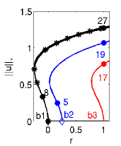
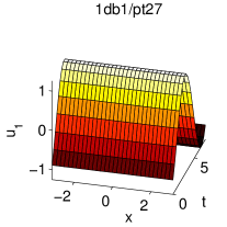
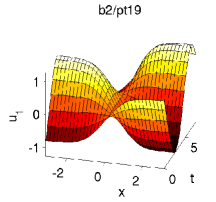
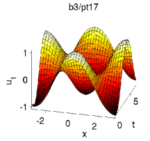
(c) BD; period $T(r)$	(d) Multipliers at b1/pt8 (${\rm ind}=1$), b1/pt27 (${\rm ind}=0$), and b2/pt5 (${\rm ind}=3$)

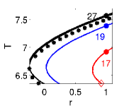
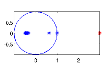
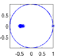
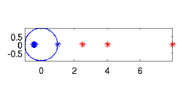
Figure 2: Numerical bifurcation diagrams, example plots and (leading 20) Floquet multipliers for (45) on the domain $\Omega=(-\pi,\pi)$ with Neumann BC, 31 grid–points in $x$. Parameters $(\nu,\mu,c_{3},c_{5})=(1,0.1,-1,1)$, hence bifurcations at (restricting to the first three branches) $r=0$ ($k=0$, spatially homogeneous branch, black), $r=1/4$ ($k=1/2$, blue) and $r=1$ ($k=1$, red), see (50). The black dots in (a), (b) are from the analytical solution (49) with $k=0$. The thick part of the black line in (a),(b) indicates the only stable periodic solutions.

On b1, initially there is one unstable multiplier $\gamma_{2}$, i.e., ${\rm ind}(u_{H})=1$, cf. (43), which passes through 1 to enter the unit circle at the fold. Its numerical value is $10^{-5}$ close to the analytical result from (51), and this error decreases upon refining the $t$–mesh. On b2 we start with ${\rm ind}(u_{H})=3$, and have ${\rm ind}(u_{H})=2$ after the fold. Near $r=0.45$ another multiplier moves through 1 into the unit circle, such that afterwards we have ${\rm ind}(u_{H})=1$, with, for instance $\gamma_{2}\approx 167$ at $r=1$. Thus, we may expect a type (i) bifurcation (cf. p. (i)) near $r=0.45$, and similarly we can identify a number of possible bifurcation on b3 and other branches. The trivial multiplier $\gamma_{1}$ is $10^{-12}$ close to $1$ in all these computations, using FA1.

The basic 1D setup has to be modified only slightly for 2D and 3D. In 2D we choose homogeneous Dirichlet BC for $u_{1},u_{2}$. Then the first two HBPs are at $r_{1}=5/4$ ($k=(1/2,1)$, and $r_{2}=2$ ($k=(1,1)$). Figure 3 shows some results obtained with a coarse mesh of $41\times 21$ points, hence $n_{u}=1722$ spatial unknowns, yielding the numerical values $r_{1}=1.2526$ and $r_{2}=2.01$. With $m=15$ temporal discretization points, the computation of each Hopf branch then takes less than a minute. Again, the numerical HBPs converge to the exact values when decreasing the mesh width, but at the prize of longer computations for the Hopf branches. For the Floquet multipliers we obtain a similar picture as in 1D. The first branch has ${\rm ind}(u_{H})=1$ up to the fold, and ${\rm ind}(u_{H})=0$ afterwards, and on b2 ${\rm ind}(u_{H})$ decreases from 3 to 2 at the fold and to 1 near $r=7.2$.

(a) BD 2D	(b) solution at b2/pt10	(c) BD 3D	(d) solution at b2/pt15

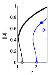
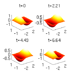
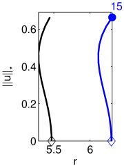
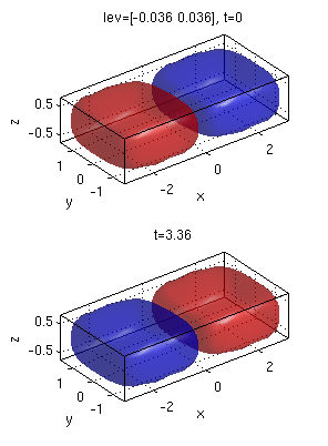
Figure 3: (a) Bifurcation diagrams of the first 2 Hopf branches for (45) in 2D. (b) Solution snapshot from b2/pt10, at $t=0,\frac{3}{10}T,\frac{6}{10}T,\frac{9}{10}T$. (c),(d) Bifurcation diagram and solution snaption in 3D

In 3D, we consider (45) over $\Omega=(-\pi,\pi)\times(-\pi/2,\pi/2)\times(-\pi/4,\pi/4)$. Here we use a very coarse tetrahedral mesh of $n_{p}=2912$ points, thus $5824$ DoF in space. Analytically, the first 2 HBPs are $r_{1}=21/4$ ($k=(1/2,1,2)$) and $r_{2}=6$ ($k=(1,1,2)$, but with the coarse mesh we numerically obtain $r_{0}=5.47$ and $r_{1}=6.29$. Again, this can be greatly improved by, e.g., halving the spatial mesh width, but then the Hopf branches become very expensive. Using $m=15$ and ilupack, the computation of the branches (with 15 continuation steps each) in Fig. 3(b) takes about 400 seconds, and using FA1 to a posteriori compute the Floquet multipliers about 30 seconds per orbit. Again, on b1, ${\rm ind}(u_{H})=1$ up to fold and ${\rm ind}(u_{H})=0$ afterwards, while on b2 ${\rm ind}(u_{H})$ decreases from 3 to 2 at the fold and to 1 at the end of the branch, and time integration from an IC from b2 yields convergence to a periodic solution from b1.

Additional to the code for the plots in Fig. 2 (and Fig. 3), the tutorial [Uec17a] explains the basic steps for

• switching to continuation in another parameter

• using pde2path’s time integration routines to assess the stability of periodic solutions, and in particular obtain the time evolution of perturbations of unstable orbits,

and some additional features such as ad hoc mesh refinement in $t$ for the arclength parametrization, and creating movies of Hopf orbits.

3.2 Rotating patterns on a disk

While the Hopf bifurcations presented in §3.1 have been to (standing) oscillatory patterns, another interesting class is the Hopf bifurcation to rotating patterns, in particular to spiral waves. Such spirals are ubiquitous in 2D reaction diffusion problems, see, e.g., [Pis06, CG09]. Over bounded domains, spiral waves are usually found numerically via time integration, see in particular EZSPIRAL [Bar91], with an ${\cal O}(1)$ amplitude, i.e., far from bifurcation. On the other hand, the bifurcation of spiral waves from a homogeneous solution is usually analyzed over all of ${\mathbb{R}}^{2}$, e.g., [Hag82, KH81, Sch98], where the spirals are relative equilibria, i.e., steady states in a comoving frame. Moreover, spiral waves often undergo secondary bifurcations such as drift, meandering and period doubling, see [Bar95, SSW99, SS07] and the references therein. An exception to the rule of finding spirals by time integration is [BE07], where they are found by growing them from a thin annulus towards the core using AUTO, i.e., by continuation in the inner radius of the annulus. Continuation in other parameters is then done as well, but always at ${\cal O}(1)$ amplitude.

Here we study, on the unit disk, the bifurcation of spiral waves from the zero solution in a slight modification of a real two component reaction diffusion system from [GKS00], somewhat similar to the cGL, but with Robin BC. The system reads

$$\begin{split}{\partial}_{t}u&=d_{1}\Delta u+(0.5+r)u+v-(u^{2}+v^{2})(u-\alpha v),\\ {\partial}_{t}v&=d_{2}\Delta v+rv-u-(u^{2}+v^{2})(v+\alpha u),\end{split}$$ (53)

$${\partial}_{{\bf n}}u+10u=0,\quad{\partial}_{{\bf n}}v+0.01v=0,$$ (54)

where ${\bf n}$ is the outer normal. First (§3.2.1) we follow [GKS00] and set $\alpha=0$, $d_{1}=0.01$, $d_{2}=0.015$, and take $r$ as the main bifurcation parameter. Then (§3.2.2) we set $\alpha=1$, let

$$(d_{1},d_{2})=\delta(0.01,0.015),$$ (55)

and also vary $\delta$ which corresponds to changing the domain size by $1/\sqrt{\delta}$.

Due to the BC (54), the eigenfunctions of the linearization around $(u,v)=(0,0)$ are build from Fourier Bessel functions

$$\phi(\rho,\vartheta,t)={\rm Re}({\rm e}^{{\rm i}(\omega t+m\vartheta)}J_{m}(q\rho)),$$ (56)

where $(\rho,\vartheta)$ are polar-coordinates, and with in general complex $q\in{\mathbb{C}}\setminus{\mathbb{R}}$. Then the modes are growing in $\rho$, which is a key idea of [GKS00] to find modes bifurcating from $(u,v)=(0,0)$ which resemble spiral waves near their core.

3.2.1 Bifurcations to rotational modes

The trivial homogeneous branch $(u,v)=(0,0)$ is stable up to $r\approx-0.21$, and Fig. 4(a) shows the first 6 bifurcating branches h1,h2,…, h6, from left to right, while (b) shows the spatial modes for h1-h6 at bifurcation, with mode numbers $m=0,1,2,3,2,4$. We discretized (53), (54) with a mesh of 1272 points, hence $n_{u}=2544$ DoF, and a coarse temporal discretization of 11 points, which yields about 2 minutes for the computation of each branch, with 10 points on each. Example plots of solutions on the last points on the branches are given in (e), with $T$ near $2\pi$ for all branches.

(a) Bifurcation diagram	(b) Spatial mode structure at bifurcation, h1,…,h6

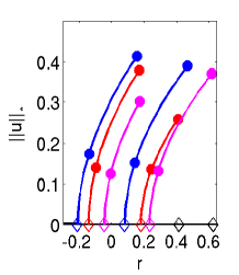
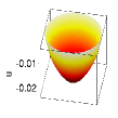
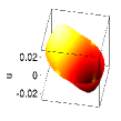
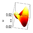
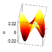
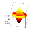
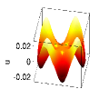
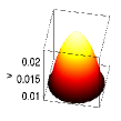
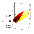
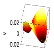
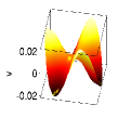
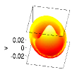
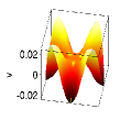
(c) Zero-contours of h2, h3, h4, h5 from (b)	(d) selected snapshots from periodic orbits

Figure 4: Basic bifurcation diagram (a) for (53), (54) with h1-h6 from left to right, 10 continuation steps for each. On each branch we mark the points 5 and 10. (b,c): information on initial mode structure on the first six bifurcating branches. (d) Example plots last points in h2, h3 (upper row) and h4, h5 (lower row). Snapshots of $u$ at $t=0,T_{j}/5$ and $2T_{j}/5$, with $T_{j}$ the actual period.

The nontrivial solutions from Fig. 4(a),(d) are “rotations”, except for the spatial $m=0$ mode h1. To discuss this, we return to (c), which shows the nodal lines for the components $u$, $v$ at bifurcation of h2 to h5 (vector $\Psi$ in (17)). The pertinent observation is that h2 to h6 (not shown) do not have nodal lines, i.e., $u(x)v(x)\neq 0$ except at $x=0$. Thus, the branches h2 to h6 cannot consist of oscillatory patterns but must rotate. On the other hand, this rotation must involve higher order modes, and thus becomes more visible, i.e., almost (but never perfectly) rigid, at larger amplitude.

To assess the numerical accuracy, in Table 1 we compare the numerical values for the Hopf points and the temporal wave number $\omega$ with the values from [GKS00], who compute $r_{4},r_{5},r_{6}$, (and three more Hopf points) using semi analytical methods, and some numerics based on the Matlab pdetoolbox with fine meshes. Given our coarse mesh we find our results reasonably close, and again our values converge to the values from [GKS00] under mesh refinement.

branch	h1	h2	h3	h4	h5	h6
$r$	-0.210	-0.141	-0.044	0.079	0.182	0.236
$\omega$	0.957	0.967	0.965	0.961	0.953	0.957
$r^{*}$	NA	NA	NA	0.080	0.179	0.234
$\omega^{*}$	NA	NA	NA	0.961	0.953	0.957
${\rm ind}(u_{H})$, pt5	0	2	6	12	16	20
${\rm ind}(u_{H})$, pt10	0	2	4	8	18	16

Table 1: Comparison of HBPs with [GKS00] (starred values), and Floquet indices at points on branches.

The last two rows of Table 1 give the Floquet indices of points on the branches, where ${\rm err}_{\gamma_{1}}$ (cf. (42)) is around $10^{-10}$ for each computation. All branches except h1 are unstable, and the instability indices increase from left to right, and also vary along the unstable branches. However, altogether (53),(54) with $(\alpha,\delta)=(0,1)$ does not appear to be very interesting from a dynamical and pattern forming point of view, as time–integration yields that for $r>r_{0}=-0.21$ solutions to generic initial conditions converge to a periodic orbit from h1. Thus, we next choose $\alpha=1$ to switch on a rotation also in the nonlinearity.

3.2.2 Spiral waves

For $(\alpha,\delta)=(1,1)$ the linearization around $(u,v)=(0,0)$ and thus also the Hopf bifurcation points $r_{h1},\ldots,r_{h6}$ are as in §3.2.1. However, the nonlinear rotation yields a spiral wave structure on the branches s2,…, s6 bifurcating at these points, see Fig. 5(b), where we only give snapshots of $u(\cdot,0)$, at $r=1$ and at $r=3$ for s2, and $r=3$ for the remaining branches. On s2 , s3, s4, and s6 the solutions rotate almost rigidly in counterclockwise direction with the indicated period $T$, while on s5 we have a clockwise rotation. Thus, on s2, s3, s4 and s6 we have inwardly moving spirals, also called anti-spirals [VE01]. Moreover, again s1 is stable for all $r>r_{h1}$, but additionally s2 becomes stable for $r>r_{1}\approx 1$, see Fig. 5(c), while s5 and the $m$–armed spirals with $m>1$ on s3, s4, s6 are unstable, as should be expected [Hag82]; also note how the core becomes flatter with an increasing number of arms, again cf. [Hag82] and the references therein.

(a) Bifurcation diagram	(b) Profiles at selected points	(c) Multipliers
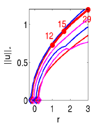
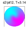
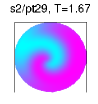
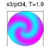
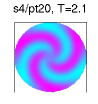
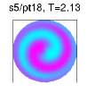
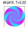
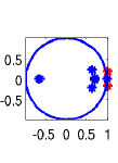
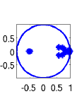
		s2/pt12 s2/pt15

Figure 5: Bifurcation diagram (a) with branches s1,…,s6 left to right, and selected profiles (b) and Floquet spectra (c). The (non–rotational) branch s1 is stable for all $r$ but plotted as a thin line (first blue line in (a)) for graphical reasons. The first two plots in (b) are both from s2, indicating the more pronounced spiral nature for larger $r$ (on all branches); remaining plots all at $r=3$. $T$ in (b) indicating the period, which decreases in $r$ and increases with number $m$ of arms of the spirals.

In Fig. 6(a) we first continue $(u,v)$ from s2 at $r=3$ in $\delta$ to $\delta=0.1$, i.e., to domain radius $\sqrt{10}$ (branch s2d). As expected, with the growing domain the spirals become more pronounced (see the example plots in (c)). The solutions stay stable down to $\delta=\delta_{1}\approx 0.15$, as illustrated in (b). In (c) we continue the solution from s2d/pt29 (with $\delta=0.2$) again in $r$ down to $r=r_{h2}^{*}\approx-0.22$, which is the associated Hopf bifurcation point over a circle of radius $\sqrt{5}$, see also the last plot in (c), which is very close to bifurcation. Now the 1-armed spiral like solution is stable also for rather small amplitude.

(a) Continuation in $\delta$, $r=3$,	(b) Multipliers	(c) Continuation in $r$, $\delta=0.2$
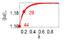
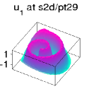
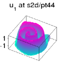
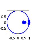
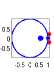
	s2d/pt29 s2d/pt44

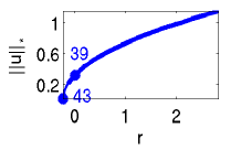
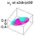
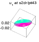
Figure 6: (a) Continuation of the one armed spiral in $\delta$ (inverse domain-size). Over a larger domain the spiral nature (of all spirals) is more visible. (b) Multipliers for points in (a). (b) Continuation of pt29 from (a) in $r$; over a larger domain the “one-armed spiral” is stable for lower amplitudes.

The model with $(r,\alpha,\delta)=(3,1,0.1)$ is also be quite rich dynamically. Besides solutions converging to s1, the 1-armed spiral s2 has a significant domain of attraction, but there are also various at least meta-stable solutions, which consist of long-lived oscillations (with or without rotations). See [Uec17a] for comments on how to run such dynamical simulations.

3.3 An extended Brusselator

As an example with an interesting interplay between stationary patterns and Hopf bifurcations, with typically many eigenvalues with small real parts, and where therefore detecting HBPs without first setting a guess for a shift $\omega_{1}$ is problematic, we consider an “extended Brusselator” problem from [YDZE02]. This is a three component reaction diffusion system of the form

$${\partial}_{t}u=D_{u}\Delta u+f(u,v)-cu+dw,\quad{\partial}_{t}v=D_{v}\Delta v+g(u,v),\quad{\partial}_{t}w=D_{w}\Delta w+cu-dw,$$ (57)

where $f(u,v)=a-(1+b)u+u^{2}v$, $g(u,v)=bu-u^{2}v$, with kinetic parameters $a,b,c,d$ and diffusion constants $D_{u},D_{v},D_{w}$. We consider (57) on rectangular domains in 1D and 2D, with homogeneous Neumann BC for all three components. The system has the trivial spatially homogeneous steady state

$$U_{s}=(u,v,w):=(a,b/a,ac/d),$$

and in suitable parameter regimes it shows co-dimension 2 points between Hopf, Turing–Hopf (aka wave), and (stationary) Turing bifurcations from $U_{s}$. We follow [YDZE02] and fix the parameters

$$(c,d,D_{u},D_{v},D_{w})=(1,1,0.01,0.1,1).$$ (58)

(a)	(b)	(c)

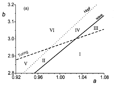
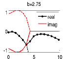
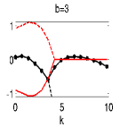
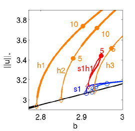
(d) solution plots

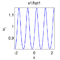
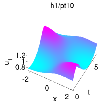
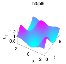
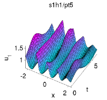
Figure 7: (a) Parameter plane with Hopf, Turing–Hopf (wave) and Turing instability lines for (57), reprinted with permission from [YDZE02], copyright 2002, AIP Publishing LLC. (b) Spectra for increasing $b$ at $a=0.95$. Contrary to the pde2path convention that due to ${\partial}_{t}u=-G(u)$ eigenvalues with negative real parts yield instabilities, here we directly plot the spectra of $-{\partial}_{u}G$, such that instability occurs for eigenvalues with positive real parts. The first instability (Turing–Hopf) occurs at $b\approx 2.794$, with $k_{c}\approx 0.7$. The admissible wave-numbers $k$ on a domain $(-l_{x},l_{x})$ with $l_{x}=0.5\pi/k_{c}$ are indicated by the dots. (c),(d): (partial) bifurcation diagram, and example plots on $\Omega=(-l_{x},l_{x})$.

Figure 7(a) then shows a characterization of the pertinent instabilities of $U_{s}$ in the $a,b$ plane. $U_{s}$ is stable in region I, and can loose stability by $(a,b)$ crossing the Turing line, which yields the bifurcation of stationary Turing patterns, or the wave (or Turing–Hopf) line, which yields oscillatory Turing patterns. Moreover, there is the “Hopf line” which corresponds to Hopf–bifurcation with spatial wave number $k=0$.

In the following we fix $a=0.95$ and take $b$ as the primary bifurcation parameter. Figure 7(b) illustrates the different instabilities from (a). As we increase $b$ from 2.75, we first cross the Turing–Hopf line, with first instability at critical spatial wave number $k_{{\rm TH}}\approx 0.7$, then the Hopf line, and finally the Turing line with critical wave number $k_{\rm T}\approx 6.4$. To investigate the bifurcating solutions (and some secondary bifurcations) with pde2path, we need to choose a domain $\Omega=(-l_{x}/2,l_{x}/2)$ (1D), where due to the Neumann BC $l_{x}$ should be chosen as a (half integer) multiple of $\pi/k_{{\rm TH}}$. For simplicity we take the minimal choice $l_{x}=0.5\pi/k_{{\rm TH}}$, which restricts the allowed wave numbers to multiples of $k_{{\rm TH}}$, as indicated by the black dots in Figure 7(b). Looking at the sequence of spectral plots for increasing $b$, we may then expect first the Turing–Hopf branch h1 with $k=k_{{\rm TH}}$, then a Hopf branch h2 with $k=0$, then two Turing branches s1, s2 with $k=6.3$ and $k=7$, then a Turing–Hopf branch h3 with $k=2k_{{\rm TH}}$, and so on, and this is what we obtain from the numerics, as illustrated in (c) and (d), using a coarse mesh with $101$ grid points, hence $3\times 101=303$ DoF in space.

Besides stationary secondary bifurcations we also get a rather large number of Hopf points on the Turing branches, and just as an example we plot the (Turing)Hopf branch s1h1 bifurcating from the first Hopf point on s1. The example plots in (d) illustrate that solutions on s1h1 look like a superposition of solutions on s1 and h1. Such solutions were already obtained in [YDZE02] from time integration, such that at least some these solutions also have some stability properties, see also [YE03] for similar phenomena. By following the model’s various bifurcations, this can be studied in a more systematic way.

(a) h1/pt10, ${\rm ind}=0$	(b) h2/pt5, ${\rm ind}=2$	(c) h2/pt10, ${\rm ind}=0$	(d) h3/pt5, ${\rm ind}=5$
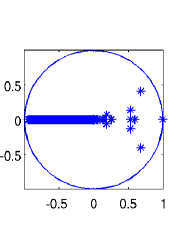
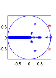
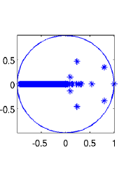
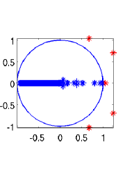
(e) “error” time series	(f) initial evolution	(g) transient near h3	(h) convergence to h1

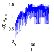
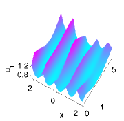
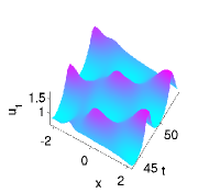
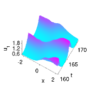
Figure 8: (a)-(d) A small sample of Floquet spectra of periodic orbits from Fig. 7 (200 largest multipliers computed via floq), illustrating that a Neimark–Sacker bifurcation should be expected near h2/pt5, and similar eigenvalue transitions occur on all other Hopf branches except h1. (e)-(h) Evolution of a perturbation of s1h1/pt10. After a rather long transient near h3 the solution converges to an orbit on h1.

In Fig. 8(a)-(d) we give some illustration that interesting bifurcations from the Hopf branches should occur in (57). It turns out that h1 is always stable, and that (the spatially homogeneous branch) h2 is initially unstable with ${\rm ind}(u_{H})=2$, but close to pt5 on h2 we find a Neimark–Sacker bifurcation, after which solutions on h2 are stable. Similarly, solutions on h3 start with ${\rm ind}(u_{H})=5$, but after a Neimark–Sacker bifurcation, and a real multiplier going through 1 at $b\approx 3.35$ we find ${\rm ind}(u_{H})=2$, before ${\rm ind}(u_{H})$ increases again for larger $b$. Also note that there are always many multipliers close to $-1$, but we did not find indications for period–doubling bifurcations. Finally, in Fig. 8(e)–(h) we illustrate the evolution of perturbations of s1h1/pt10. After a transient near h3/pt5 (g) the solution converges to a solution from the primary Hopf branch h1 (h), which however itself also shows some short wave structure at this relatively large distance from bifurcation.

In 1D we may still use HD1 to detect (and localize) the Hopf bifurcations. In 2D this is unfeasible, because even over rather small domains we obtain many wave vectors $k=(k_{1},k_{2})$ with modulus $|k|\in(5,8)$, which give leading eigenvalues $\mu_{1}(k)$ with small ${\rm Re}\mu(k)$ and ${\rm Im}\mu(k)=0$. This is illustrated in Fig. 9, which shows that for $\Omega=(-0.5\pi/k_{{\rm TH}},0.5\pi/k_{{\rm TH}})^{2}$ even for $n_{\text{eig}}=200$ (which is quite slow already) we do not even see any Hopf eigenvalues, which become “visible” at, e.g., $n_{\text{eig}}=300$. Thus, here we use HD2 which runs fast and reliably, even with just computing 3 eigenvalues both near 0 and $\omega_{1}$, obtained from (12).

(a) $n_{\text{eig}}=200$	(b) $n_{\text{eig}}=300$	(c) $|g|$ from (12)	(d) $n_{\text{eig}}=(3,3)$ with $\omega_{1}=0.9375$

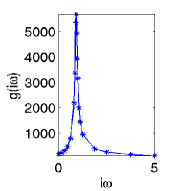
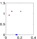
Figure 9: (a,b) $n_{\text{eig}}$ smallest eigenvalues of the linearization of (57) around $U_{s}$ at $b=2.75$, remaining parameters from (58); HD1  with $n_{\text{eig}}=200$ will not detect any Hopf points. (c) (12) yields a guess $\omega_{1}=0.9375$ for the $\omega$ value at Hopf bifurcation, and then HD2 with $n_{\text{eig}}=(3,3)$ is reliable and fast: (d) shows the three eigenvalues closest to $0$ in blue, and the three eigenvalues closest to ${\rm i}\omega_{1}$ in red.

Finally, in Fig. 10 we give an example of just four of the many branches which can be obtained for (57) in 2D, even over quite small domains. We use $\Omega=(-l_{x},l_{x})\times(-l_{y},l_{y})$, $l_{x}=\pi/2$, $l_{y}=\pi/8$, where we start wish a mesh of 961 gridpoints, hence 2883 spatial degrees of freedom. The domain means that admissible wave vectors are $(k_{1},k_{2})=(n,4m)$, $n,m\in{\mathbb{N}}_{0}$. Consequently, no spatial structure in $y$ direction occurs in the primary Hopf branches (cf. Fig. 7b), i.e., the first three are just analogous to those in Fig. 7 and occur at $b=2.818$ (with $k=(1,0)$), $b=2.859$ (with $k=(0,0)$, i.e., spatially homogeneous, and hence $b$ independent of the domain) and $b=3.202$ (with $k=(2,0)$); see (b1) for an example plot on the first Hopf branch. The first stationary bifurcation (at $b=2.912$) is now to a spotted branch 2ds1, and stripe branches analogous to s1 from Fig. 7 bifurcate at larger $b$. Interestingly, after some stationary and Hopf bifurcations the 2ds1 branch becomes stable at $b=b_{b}\approx 2.785$, which illustrates that it is often worthwhile to follow unstable branches, as they may become stable, or stable branches may bifurcate off. Figure 10(b2) shows an example plot from the first secondary Hopf branch. This is analogous to s1h1 from Fig. 7, i.e., the solutions look like superpositions of the stationary pattern and solutions on the primary Hopf branch h1. Concerning the multipliers we find that ${\rm ind}(u_{H})=0$ on 2dh1, and, e.g., ${\rm ind}(u_{H})=5$ at 2ds1h1/pt5, where as in 1D (Fig. 9) there are multipliers suggesting Neimark–Sacker bifurcations. Figure 10 (c) illustrates the instability of the spotted Hopf solutions; the spots stay visible for about 4 periods, and subsequently the solution converges to a periodic orbit from the primary Hopf branch, as in Fig. 8.

(a) BD, and $u$ at first HBP on 2ds1 branch	(b) Hopf example plots ($u$)	(c) Convergence to the primary Hopf branch 2dh1
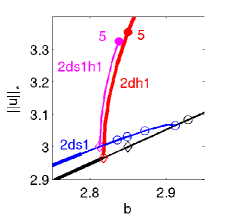
	1) 2dh1/pt5 at $t=0,T/2$ 2) 2ds1h1/pt5 at $t{=}0,\ldots,3T/4$

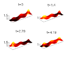
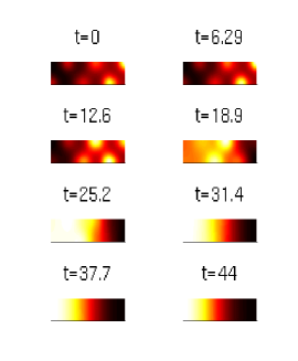
Figure 10: (a) Example bifurcations for (57) over a small 2D domain $\Omega=(-\pi/2,\pi/2)\times(-\pi/8,\pi/8)$, and example plots of $u$ at 2nd Hopf point on the blue branch. (b) Example plots: solutions on primary Hopf branch (1), and on the secondary Hopf branch (2) (the amplitude at $t=1.4$ and $t=4.19$ is about 0.2). (c) Time integration with $u(\cdot,0)$ from 2ds1h1/pt5, snapshots at $0,T,2T,\ldots,8T$.

3.4 A canonical system from optimal control

In [Uec16, GU17], pde2path has been used to study so called canonical steady states and canonical paths for infinite time horizon distributed optimal control (OC) problems. As an example for such problems with Hopf bifurcations we consider

$$V(v_{0}(\cdot))\stackrel{{\scriptstyle!}}{{=}}\max_{k(\cdot,\cdot)}J(v_{0}(\cdot),k(\cdot,\cdot)),\qquad J(v_{0}(\cdot),k(\cdot,\cdot)):=\int_{0}^{\infty}{\rm e}^{-\rho t}J_{ca}(v(t),k(t))\,{\rm d}t,$$ (59a)

where $$J_{ca}(v(\cdot,t),k(\cdot,t))=\frac{1}{|\Omega|}\int_{\Omega}J_{c}(v(x,t),k(x,t))\,{\rm d}x$$ is the spatially averaged current value function, with

$$J_{c}(v,k)=pv_{1}-\beta v_{2}-C(k)\text{ the local current value,}\quad C(k)=k+\frac{1}{2\gamma}k^{2},$$ (59b)

$$\rho>0$$ is the discount rate (long-term investment rate), and where the state evolution is

$${\partial}_{t}v_{1}=-k+d_{1}\Delta v_{1},\quad{\partial}_{t}v_{2}=v_{1}-\alpha(v_{2})+d_{2}\Delta v_{2},$$ (59c)

with Neumann BC ${\partial}_{\bf n}v=0$ on ${\partial}\Omega$. Here, $v_{1}=v_{1}(t,x)$ are the emissions of some firms, $v_{2}=v_{2}(t,x)$ is the pollution stock, and the control $k=k(t,x)$ models the firms’ abatement policies. In $J_{c}$, $pv_{1}$ and $\beta v_{2}$ are the firms’ value of emissions and costs of pollution, $C(k)$ are the costs for abatement, and $\alpha(v_{2})=v_{2}(1-v_{2})$ is the recovery function of the environment. The discounted time integral in (59a) is typical for economic problems, where “profits now” weight more than mid or far future profits. Finally, the $\max$ in (59a) runs over all admissible controls $k$; this essentially means that $k\in L^{\infty}((0,\infty)\times\Omega,{\mathbb{R}})$, and we do not consider active control or state constraints.

The associated ODE OC problem (no $x$–dependence of $v,k$) was set up and analyzed in [TW96, Wir00]; in suitable parameter regimes it shows Hopf bifurcations of periodic orbits for the associated so called canonical (ODE) system. See also, e.g., [DF91, Wir96, GCF⁺08] for general results about the occurrence of Hopf bifurcations and optimal periodic solutions in ODE OC problems.

Setting $g_{1}(v,k)=(-k,v_{1}-\alpha(v_{2}))^{T}$, and introducing the co–states (Lagrange multipliers)

$$\lambda:\Omega\times(0,\infty)\rightarrow{\mathbb{R}}^{2}$$

and the (local current value) Hamiltonian ${\cal H}={\cal H}(v,\lambda,k)=J_{c}(v,k)+\left\langle\lambda,D\Delta v+g_{1}(v,k)\right\rangle$, by Pontryagin’s Maximum Principle for $\tilde{{\cal H}}=\int_{0}^{\infty}{\rm e}^{-\rho t}{\overline{{\cal H}}}(t)\,{\rm d}t$ with ${\overline{{\cal H}}}(t)=\int_{\Omega}{\cal H}(v(x,t),\lambda(x,t),k(x,t))\,{\rm d}x$, an optimal solution $(v,\lambda)$ has to solve the canonical system (first order necessary optimality conditions)

$${\partial}_{t}v ={\partial}_{\lambda}{\cal H}=D\Delta v+g_{1}(v,k),\quad v|_{t=0}=v_{0},$$ (60a)

$${\partial}_{t}\lambda =\rho\lambda-{\partial}_{v}{\cal H}=\rho\lambda+g_{2}(v,k)-D\Delta\lambda,$$ (60b)

where ${\partial}_{\bf n}\lambda=0$ on ${\partial}\Omega$. The control $k$ fulfills $k{=}\operatornamewithlimits{argmax}_{\tilde{k}}{\cal H}(v,\lambda,\tilde{k})$, and under suitable concavity assumptions on $J_{c}$ and in the absence of control constraints is obtained from solving ${\partial}_{k}{\cal H}(v,\lambda,k){=}0$, thus here

$$k=k(\lambda_{1})=-(1+\lambda_{1})/\gamma.$$ (61)

Note that (60) is ill–posed as an initial value problem due to the backward diffusion in the co–states $\lambda$. Thus it seems unlikely that periodic orbits for (60) can be obtained via shooting methods. For convenience we set $u(t,\cdot):=(v(t,\cdot),\lambda(t,\cdot)):\Omega\rightarrow{\mathbb{R}}^{4}$, and write (60) as

$${\partial}_{t}u=-G(u):={\cal D}\Delta u+f(u),$$ (62)

where $\displaystyle{\cal D}=$diag$(d_{1},d_{2},-d_{1},-d_{2})$, $\displaystyle f(u)=\biggl{(}-k,v_{1}-\alpha(v_{2}),\rho\lambda_{1}-p-\lambda_{2},(\rho+\alpha^{\prime}(v_{2}))\lambda_{2}+\beta\biggr{)}^{T}$. Besides the boundary condition ${\partial}_{\bf n}u=0$ on ${\partial}\Omega$ and the initial condition $v|_{t=0}=v_{0}$ (only) for the states, we have the so called intertemporal transversality condition

$$\lim_{t\to\infty}{\rm e}^{-\rho t}\int_{\Omega}\left\langle v,\lambda\right\rangle\,{\rm d}x=0,$$ (63)

which was already used in the derivation of (60).

A solution $u$ of the canonical system (62) is called a canonical path, and a steady state of (62) (which automatically fulfills (63)) is called a canonical steady state (CSS). A first step for OC problems of type (59) is to find canonical steady states and canonical paths connecting to some CSS $u^{*}$. To find such connecting orbits to $u^{*}$ we may choose a cut–off time $T_{1}$ and require that $u(\cdot,T_{1})$ is in the stable manifold $W_{s}(u^{*})$ of $u^{*}$, which we approximate by the associated stable eigenspace $E_{s}(u^{*})$. If we consider (60) after spatial discretization, then, since we have $n_{u}/2$ initial conditions, this requires that $\dim E_{s}(u^{*})=n_{u}/2$. Defining the defect $d(u^{*})$ of a CSS as

$$d(u^{*})=\frac{n_{u}}{2}-\dim E_{s}(u^{*}),$$ (64)

it turns out (see [GU16, Appendix A]) that always $d(u^{*})\geq 0$, and we call a $u^{*}$ with $d(u^{*})=0$ a saddle–point CSS. See [GCF⁺08, GU16] for more formal definitions, and further comments on the notions of optimal systems, the significance of the transversality condition (63), and the (mesh-independent) defect $d(u^{*})$. For a saddle point CSS $u^{*}$ we can then compute canonical paths to $u^{*}$, and this has for instance been carried out for a vegetation problem in [Uec16], with some surprising results, including the bifurcation of patterned optimal steady states and optimal paths.

A natural next step is to search for time–periodic solutions $u_{H}$ of canonical systems, which obviously also fulfill (63). The natural generalization of (64) is

$$d(u_{H})={\rm ind}(u_{H})-\frac{n_{u}}{2}.$$ (65)

In the (low–dimensional) ODE case, there then exist methods to compute connecting orbits to (saddle point) periodic orbits $u_{H}$ with $d(u_{H})=0$, see [BPS01, GCF⁺08], which require comprehensive information on the Floquet multipliers and the associated eigenspace of $u_{H}$. Our (longer term) aim is to extend these methods to periodic orbits of PDE OC systems.

However, a detailed numerical analysis of (59) and similar PDE optimal control problems with Hopf bifurcations, and economic interpretation of the results, will appear elsewhere. Here we only illustrate that

• Hopf orbits can appear as candidates for optimal solutions in OC problems of the form (59),

• the computation of multipliers via the periodic Schur decomposition (FA2) can yield accurate results, even when the computation directly based on the product (41) (FA1) completely fails.

For all parameter values, (62) has the spatially homogeneous CSS

$$u^{*}=(z_{*}(1-z_{*}),z_{*},-1,-(p+\rho)),\quad\text{where}\quad z_{*}=\frac{1}{2}\left(1+\rho-\frac{\beta}{p+\rho}\right).$$

We use similar parameter ranges as in [Wir00], namely

$$(p,\beta,\gamma)=(1,0.2,300),\text{ and }\rho\in[0.5,0.65]\text{ as a continuation parameter},$$ (66)

consider (62) over $\Omega=(-\pi/2,\pi/2)$, and set the diffusion constants to $d_{1}=0.001,d_{2}=0.2$. In Figure 11 we give some basic results for (62) with a coarse spatial discretization of $\Omega$ by only $n_{p}=41$ points (and thus $n_{u}=164$). (a) shows the full spectrum of the linearization of (62) around $u^{*}$ at $\rho=0.5$, illustrating the ill-posedness of (62) as an initial value problem. (b) shows a basic bifurcation diagram. At $\rho=\rho_{1}\approx 0.53$ there bifurcates a Hopf branch h1 with spatial wave number $l=1$, and at $\rho=\rho_{2}\approx 0.58$ a spatially homogeneous ($l=0$) Hopf branch h2 bifurcates subcritically with a fold at $\rho=\rho_{f}\approx 0.55$. (c) shows the pertinent time series on h2/pt14. As should be expected, $J_{c}$ is large when the pollution stock is low and emissions are high, and the pollution stock follows the emissions with some delay.

(a) spectrum of ${\partial}_{u}G(u^{*})$, $\rho=0.5$	(b) bif. diagram	(c) time series on h2/pt14 (spat. homogen. branch)
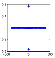
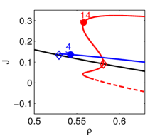
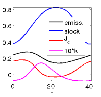
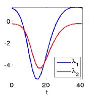
(d) example plots at h1/pt4
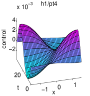
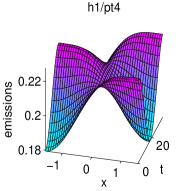
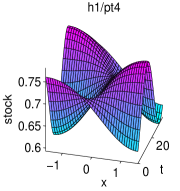
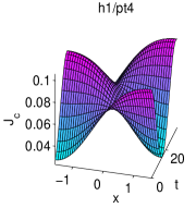
(f) the $\frac{n_{u}}{2}$ smallest $\gamma_{j}$ at h2/pt4	(g) $|\gamma_{j}|$ for the $\frac{n_{u}}{2}$ largest $\gamma_{j}$ at h2/pt4	(h) the $\frac{n_{u}}{2}$ smallest $\gamma_{j}$ at h2/pt4 and at h2/pt14

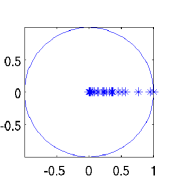
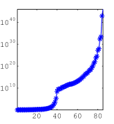
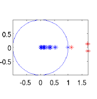
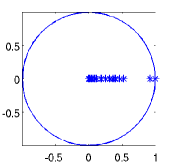
Figure 11: (a) full spectrum of the linearization of (62) around $u^{*}$ at $\rho=0.5$ on a coarse mesh with $n_{p}=17$. (b) Bifurcation diagram, value $J$ over $\rho$. Black: $u^{*}$; blue: h1, red: h2, $J(u^{H};0)$ (full line) and $J(u^{H};T/2)$ (dashed line). (c) Time series of a spatially homogeneous solution, including current value $J_{c}$, control $k$, and co–states $\lambda_{1,2}$. (d,f,g) Example plots and and multipliers of $u_{H}$ at h1/pt4, which shows that ${\rm ind}(u_{H})=0$. (h) multipliers at h2/pt4, which shows that ${\rm ind}(u_{H})=3$ at this point, while solutions on h2 become saddles after the fold.

Since ultimately we are interested in the values $J$ of solutions of (62), in (b) we plot $J$ over $\rho$. For the CSS $u^{*}$ this is simply $J(u^{*})=\frac{1}{\rho}J_{c,a}(u^{*})$, but for the periodic orbits we have to take into account the phase, which is free for (62). If $u_{H}$ is a time periodic solution of (62), then, for $\phi\in[0,T)$, we consider

$$J(u_{H};\phi):=\int_{0}^{\infty}{\rm e}^{-\rho t}J_{c,a}(u_{H}(t+\phi))\,{\rm d}t=\frac{1}{1-{\rm e}^{-\rho T}}\int_{0}^{T}{\rm e}^{-\rho t}J_{c,a}(u_{H}(t+\phi))\,{\rm d}t,$$

which in general may depend on the phase, and for h2 in (c) we plot $J(u_{H};\phi)$ for $\phi=0$ (full red line) and $\phi=T/2$ (dashed red line). For the spatially periodic branch h1, $J_{c,a}(t)$ averages out in $x$ and hence $J(u_{H};\phi)$ only weakly depends on $\phi$. Thus, we first conclude that for $\rho\in(\rho_{1},\rho_{f})$ the spatially patterned periodic orbits from h1 give the highest $J$, while for $\rho\geq\rho_{f}$ this is obtained from h2 with the correct phase. The example plots (c) at h1/pt4 illustrate how the spatio-temporal dependence of $k$ should be chosen, and the resulting behaviors of $v$ and $J_{c}$.

It remains to compute the defects $d(u^{*})$ of the CSS and $d(u_{H})$ of periodic orbits on the bifurcating branches. For $d(u^{*})$ we find that it starts with $0$ at $\rho=0.5$, and, as expected, increases by 2 at each Hopf point. On the Hopf branches we always have $n_{+}\geq n_{u}/2$ unstable multipliers (computed with FA2, which yields ${\rm err}_{\gamma_{1}}<10^{-8}$ for all computations, and hence we trust it), and the leading multipliers are very large, i.e., on the order of $10^{40}$, even for the coarse space discretization. Thus, we may expect FA1 to fail, and indeed it does so completely. For instance, calling floq to compute all multipliers typically returns 10 and larger for the modulus of the smallest multiplier (which from FA2 is on the order of $10^{-25}$).

On h1 we find $d(u_{H})=0$ up to pt4, see (e) for the $n_{u}/2$ smallest multipliers, and (f) for $|\gamma_{j}|$ for the large ones, which are mostly real, and $d(u_{H})\geq 1$ for larger $\rho$. On h2 we start with $d(u_{H})=3$, see (h), but $d(u_{H})=0$ after the fold until $\rho=\rho_{1}\approx 0.6$, after which $d(u_{H})$ increases again by multipliers going though 1. Since on h1 we have that $J(u_{H})$ is larger than $J(u^{*})$, and since $u_{H}$ is a saddle point up to pt4, we expect that these $u_{H}$ are at least locally optimal, and similarly we expect $u_{H}$ from h2 after the fold until $\rho_{1}$ to be locally, and probably globally, optimal. However, as already said, for definite answers and, e.g., to characterize the domains of attractions, we need to compute canonical paths connecting to these periodic orbits, and this will be studied elsewhere.

4 Summary and outlook

With the hopf library of pde2path we provide basic functionality for Hopf bifurcations and periodic orbit continuation for the class (3) of PDEs over 1D, 2D and 3D domains. The user interfaces reuse the standard pde2path setup, and no new user functions are necessary. For the detection of Hopf points we check for eigenvalues crossing the imaginary axis near guesses ${\rm i}\omega_{j}$, where the $\omega_{j}$ can either be set by the user (if such a priori information is available), or can be estimated using the function $g$ from (12). An initial guess for a bifurcating periodic orbit is then obtained from the normal form (13), and the continuation of the periodic orbits is based on modifications of routines from TOM [MT04].

Floquet multipliers of periodic orbits can be computed from the monodromy matrix ${\cal M}$ (41) (FA1), or via a periodic Schur decomposition of the block matrices of ${\cal M}$ (FA2). The former is suitable for dissipative systems, and computes a user chosen number of largest multipliers of ${\cal M}$. This definitely fails for problems of the type considered in §3.4, and in general we recommend to monitor ${\rm err}_{\gamma_{1}}=|\gamma_{1}-1|$ to detect further possible inaccuracies. The periodic Schur decomposition is expensive, but has distinct advantages: It can be used to efficiently compute eigenspaces at all time–slices and hence bifurcation information in case of critical multipliers, and, presently most importantly for us, it accurately (measured by ${\rm err}_{\gamma_{1}}$) computes the multipliers also for ill posed evolution problems.

We tested our algorithms on four example problems, where we believe that the second, third and fourth are close to interesting research problems. For instance, the numerical results on (53),(54) seem to be the first on bifurcation of spiral waves out of zero over a bounded domain, in a reaction diffusion system without very special boundary conditions. Further interesting problems will be, e.g., the bifurcation from Hopf branches in this model, and in (57). Thus, as one next step we plan to implement the necessary localization and branch switching routines, for which the cGL equation (44) will again provide a good test case. In §3.4 we give a (very basic) illustration of the widely unexplored field of Hopf bifurcations and time periodic orbits in infinite time horizon distributed optimal control PDE problems. For this, as a next step we plan to implement routines to compute canonical paths connecting to periodic orbits.

Finally, another interesting field are Hopf bifurcations from traveling waves, or more generally in systems with continuous symmetries, see Remark 2.1. Examples how to treat these in pde2path, based on the setup presented here with minor additions, are given in [RU17, §4] and [Uec17b, §5].

References

- [AK02] I. S. Aranson and L. Kramer. The world of the complex Ginzburg-Landau equation. Rev. Modern Phys., 74(1):99–143, 2002.
- [Bar91] D. Barkley. Computer simulation of waves in excitable media. Physica D, pages 61–70, 1991.
- [Bar95] D. Barkley. Spiral meandering. In Chemical Waves and Patterns, edited by R. Kapral and K. Showalter, page 163. Kluwer, 1995.
- [BE07] G. Bordyugov and H. Engel. Continuation of spiral waves. Physica D, pages 49–58, 2007.
- [BGVD92] A. Bojanczyk, G.H. Golub, and P. Van Dooren. The periodic Schur decomposition; algorithm and applications. In Proc. SPIE Conference, Volume 1770, pages 31–42. 1992.
- [Bol11] M. Bollhöfer. ILUPACK V2.4, www.icm.tu-bs.de/bolle/ilupack/, 2011.
- [BPS01] W.J. Beyn, Th. Pampel, and W. Semmler. Dynamic optimization and Skiba sets in economic examples. Optimal Control Applications and Methods, 22(5–6):251–280, 2001.
- [BT07] W.J. Beyn and V. Thümmler. Phase conditions, symmetries, and pde continuation. In Numerical continuation methods for dynamical systems, pages 301–330. Springer, Dordrecht, 2007.
- [BT10] Ph. Beltrame and U. Thiele. Time integration and steady-state continuation for 2d lubrication equations. SIAM J. Appl. Dyn. Syst., 9(2):484–518, 2010.
- [CG09] M. Cross and H. Greenside. Pattern Formation and Dynamics in Nonequilibrium Systems. Cambridge University Press, 2009.
- [DF91] E. Dockner and G. Feichtinger. On the optimality of limit cycles in dynamic economic systems. Journal of Economics, 53:31–50, 1991.
- [Doe07] E. J. Doedel. Lecture notes on numerical analysis of nonlinear equations. In Numerical continuation methods for dynamical systems, pages 1–49. Springer, Dordrecht, 2007.
- [DRUW14] T. Dohnal, J. Rademacher, H. Uecker, and D. Wetzel. pde2path 2.0. In H. Ecker, A. Steindl, and S. Jakubek, editors, ENOC 2014 - Proceedings of 8th European Nonlinear Dynamics Conference, ISBN: 978-3-200-03433-4, 2014.
- [DU16] T. Dohnal and H. Uecker. Bifurcation of Nonlinear Bloch waves from the spectrum in the nonlinear Gross-Pitaevskii equation. J. Nonlinear Sci., 26(3):581–618, 2016.
- [DWC+14] H. A. Dijkstra, F. W. Wubs, A. K. Cliffe, E. Doedel, I. Dragomirescu, B. Eckhardt, A. Yu. Gelfgat, A. L. Hazel, V. Lucarini, A. G. Salinger, E. T. Phipps, J Sanchez-Umbria, H Schuttelaars, L. S. Tuckerman, and U. Thiele. Numerical bifurcation methods and their application to fluid dynamics: Analysis beyond simulation. Communications in Computational Physics, 15:1–45, 2014.
- [dWDR+17] H. de Witt, T. Dohnal, J. Rademacher, H. Uecker, and D. Wetzel. pde2path - Quickstart guide and reference card, 2017. Available at [Uec17c].
- [EWGT17] S. Engelnkemper, M. Wilczek, S. Gurevich, and U. Thiele. Morphological transitions of sliding drops - dynamics and bifurcations. Phys-Rev.Fluids, (1, 073901), 2017.
- [FJ91] Th. F. Fairgrieve and A. D. Jepson. O. K. Floquet multipliers. SIAM J. Numer. Anal., 28(5):1446–1462, 1991.
- [GAP06] S. V. Gurevich, Sh. Amiranashvili, and H.-G. Purwins. Breathing dissipative solitons in three-component reaction-diffusion system. Phys. Rev. E, 74:066201, 2006.
- [GCF+08] D. Grass, J.P. Caulkins, G. Feichtinger, G. Tragler, and D.A. Behrens. Optimal Control of Nonlinear Processes: With Applications in Drugs, Corruption, and Terror. Springer Verlag, 2008.
- [GF13] S. V. Gurevich and R. Friedrich. Moving and breathing localized structures in reaction-diffusion system. Math. Model. Nat. Phenom., 8(5):84–94, 2013.
- [GKS00] M. Golubitsky, E. Knobloch, and I. Stewart. Target patterns and spirals in planar reaction-diffusion systems. J. Nonlinear Sci., 10(3):333–354, 2000.
- [Gov00] W. Govaerts. Numerical methods for bifurcations of dynamical equilibria. SIAM, 2000.
- [GS96] W. Govaerts and A. Spence. Detection of Hopf points by counting sectors in the complex plane. Numer. Math., 75(1):43–58, 1996.
- [GU16] D. Grass and H. Uecker. Optimal management and spatial patterns in a distributed shallow lake model. Preprint, 2016.
- [GU17] D. Grass and H. Uecker. Optimal management and spatial patterns in a distributed shallow lake model. Electr. J. Differential Equations, 2017(1):1–21, 2017.
- [Hag82] P.S. Hagan. Spiral waves in reaction-diffusion equations. SIAM Journal on Applied Mathematics, 42:762–786, 1982.
- [HM94] A. Hagberg and E. Meron. Pattern formation in non-gradient reaction-diffusion systems: the effects of front bifurcations. Nonlinearity, 7:805–835, 1994.
- [KH81] N. Kopell and L.N. Howard. Target pattern and spiral solutions to reaction-diffusion equations with more than one space dimension. Advances in Applied Mathematics, 2(4):417–449, 1981.
- [Kre01] D. Kressner. An efficient and reliable implementation of the periodic qz algorithm. In IFAC Workshop on Periodic Control Systems. 2001.
- [Kre06] D. Kressner. A periodic Krylov-Schur algorithm for large matrix products. Numer. Math., 103(3):461–483, 2006.
- [Küh15a] Chr. Kühn. Efficient gluing of numerical continuation and a multiple solution method for elliptic PDEs. Appl. Math. Comput., 266:656–674, 2015.
- [Küh15b] Chr. Kühn. Numerical continuation and SPDE stability for the 2D cubic-quintic Allen-Cahn equation. SIAM/ASA J. Uncertain. Quantif., 3(1):762–789, 2015.
- [Kuz04] Yu. A. Kuznetsov. Elements of applied bifurcation theory, volume 112 of Applied Mathematical Sciences. Springer-Verlag, New York, third edition, 2004.
- [LR00] K. Lust and D. Roose. Computation and bifurcation analysis of periodic solutions of large-scale systems. In Numerical methods for bifurcation problems and large-scale dynamical systems (Minneapolis, MN, 1997), volume 119 of IMA Vol. Math. Appl., pages 265–301. Springer, New York, 2000.
- [LRSC98] K. Lust, D. Roose, A. Spence, and A. R. Champneys. An adaptive Newton-Picard algorithm with subspace iteration for computing periodic solutions. SIAM J. Sci. Comput., 19(4):1188–1209, 1998.
- [Lus01] K. Lust. Improved numerical Floquet multipliers. Internat. J. Bifur. Chaos, 11(9):2389–2410, 2001.
- [Mei00] Z. Mei. Numerical bifurcation analysis for reaction-diffusion equations. Springer-Verlag, Berlin, 2000.
- [Mie02] A. Mielke. The Ginzburg-Landau equation in its role as a modulation equation. In Handbook of dynamical systems, Vol. 2, pages 759–834. North-Holland, 2002.
- [MT04] F. Mazzia and D. Trigiante. A hybrid mesh selection strategy based on conditioning for boundary value ODE problems. Numerical Algorithms, 36(2):169–187, 2004.
- [NS15] M. Net and J. Sánchez. Continuation of bifurcations of periodic orbits for large-scale systems. SIAM J. Appl. Dyn. Syst., 14(2):674–698, 2015.
- [Pis06] L.M. Pismen. Patterns and interfaces in dissipative dynamics. Springer, 2006.
- [RU17] J. Rademacher and H. Uecker. Symmetries, freezing, and Hopf bifurcations of modulated traveling waves in pde2path, 2017.
- [Sch98] A. Scheel. Bifurcation to spiral waves in reaction-diffusion systems. SIAM journal on mathematical analysis, 29(6):1399–1418, 1998.
- [SDE+15] E. Siero, A. Doelman, M. B. Eppinga, J. D. M. Rademacher, M. Rietkerk, and K. Siteur. Striped pattern selection by advective reaction-diffusion systems: resilience of banded vegetation on slopes. Chaos, 25(3), 2015.
- [Sey10] R. Seydel. Practical bifurcation and stability analysis. 3rd ed. Springer, 2010.
- [SGN13] J. Sánchez, F. Garcia, and M. Net. Computation of azimuthal waves and their stability in thermal convection in rotating spherical shells with application to the study of a double-hopf bifurcation. Phys. Rev. E, page 033014, 2013.
- [SS07] B. Sandstede and A. Scheel. Period-doubling of spiral waves and defects. SIAM J. Appl. Dyn. Syst., 6(2):494–547, 2007.
- [SSW99] B. Sandstede, A. Scheel, and C. Wulff. Bifurcations and dynamics of spiral waves. J. Nonlinear Sci., 9(4):439–478, 1999.
- [TB00] L. S. Tuckerman and D. Barkley. Bifurcation analysis for timesteppers. In Numerical methods for bifurcation problems and large-scale dynamical systems (Minneapolis, MN, 1997), volume 119 of IMA Vol. Math. Appl., pages 453–466. Springer, New York, 2000.
- [TW96] O. Tahvonen and C. Withagen. Optimality of irreversible pollution accumulation. Journal of Environmental Economics and Management, 20:1775–1795, 1996.
- [Uec16] H. Uecker. Optimal harvesting and spatial patterns in a semi arid vegetation system. Natural Resource Modelling, 29(2):229–258, 2016.
- [Uec17a] H. Uecker. Hopf bifurcation and time periodic orbits with pde2path – a tutorial, 2017. Available at [Uec17c].
- [Uec17b] H. Uecker. Hopf bifurcation and time periodic orbits with pde2path – a tutorial, 2017.
- [Uec17c] H. Uecker. www.staff.uni-oldenburg.de/hannes.uecker/pde2path, 2017.
- [UW14] H. Uecker and D. Wetzel. Numerical results for snaking of patterns over patterns in some 2D Selkov-Schnakenberg Reaction-Diffusion systems. SIADS, 13-1:94–128, 2014.
- [UW17] H. Uecker and D. Wetzel. The pde2path linear system solvers – a tutorial, 2017. Available at [Uec17c].
- [UWR14] H. Uecker, D. Wetzel, and J. Rademacher. pde2path – a Matlab package for continuation and bifurcation in 2D elliptic systems. NMTMA, 7:58–106, 2014.
- [VE01] V. K. Vanag and I. R. Epstein. Inwardly rotating spiral waves in a reaction–diffusion system. Science, 294, 2001.
- [Wet16] D. Wetzel. Pattern analysis in a benthic bacteria-nutrient system. Math. Biosci. Eng., 13(2):303–332, 2016.
- [WIJ13] I. Waugh, S. Illingworth, and M. Juniper. Matrix-free continuation of limit cycles for bifurcation analysis of large thermoacoustic systems. J. Comput. Phys., 240:225–247, 2013.
- [Wir96] Fr. Wirl. Pathways to Hopf bifurcation in dynamic, continuous time optimization problems. Journal of Optimization Theory and Applications, 91:299–320, 1996.
- [Wir00] Fr. Wirl. Optimal accumulation of pollution: Existence of limit cycles for the social optimum and the competitive equilibrium. Journal of Economic Dynamics and Control, 24(2):297–306, 2000.
- [YDZE02] L. Yang, M. Dolnik, A. M. Zhabotinsky, and I. R. Epstein. Pattern formation arising from interactions between Turing and wave instabilities. J. Chem. Phys., 117(15):7259–7265, 2002.
- [YE03] L. Yang and I. R. Epstein. Oscillatory Turing patterns in reaction–diffusion systems with two coupled layers. PRL, 90(17):178303–1–4, 2003.
- [ZHKR15] D. Zhelyazov, D. Han-Kwan, and J. D. M. Rademacher. Global stability and local bifurcations in a two-fluid model for tokamak plasma. SIAM J. Appl. Dyn. Syst., 14(2):730–763, 2015.
- [ZUFM17] Y. Zelnik, H. Uecker, U. Feudel, and E. Meron. Desertification by front propagation? Journal of Theoretical Biology, pages 27–35, 2017.