Parquet decomposition calculations of the electronic self-energy

Abstract

The parquet decomposition of the self-energy into classes of diagrams, those associated with specific scattering processes, can be exploited for different scopes. In this work, the parquet decomposition is used to unravel the underlying physics of non-perturbative numerical calculations. We show the specific example of dynamical mean field theory (DMFT) and its cluster extensions (DCA) applied to the Hubbard model at half-filling and with hole doping: These techniques allow for a simultaneous determination of two-particle vertex functions and self-energies, and hence, for an essentially “exact” parquet decomposition at the single-site or at the cluster level. Our calculations show that the self-energies in the underdoped regime are dominated by spin scattering processes, consistent with the conclusions obtained by means of the fluctuation diagnostics approach [Phys. Rev. Lett. 114, 236402 (2015)]. However, differently from the latter approach, the parquet procedure displays important changes with increasing interaction: Even for relatively moderate couplings, well before the Mott transition, singularities appear in different terms, with the notable exception of the predominant spin-channel. We explain precisely how these singularities, which partly limit the utility of the parquet decomposition, and - more generally - of parquet-based algorithms, are never found in the fluctuation diagnostics procedure. Finally, by a more refined analysis, we link the occurrence of the parquet singularities in our calculations to a progressive suppression of charge fluctuations and the formation of an RVB state, which are typical hallmarks of a pseudogap state in DCA.

I Introduction

Traditionally, the electron self-energy is often determined via diagram expansion methods.Hedin ; AGD Diagrams to low order in the interaction strength can be calculated in perturbation theory. It may also be possible to sum certain classes of diagrams to infinite order. For instance, the lowest order diagram in the screened Coulomb interaction, the GW method,GW gives reasonable results for moderately correlated systems, such as free-electron-like metals and semiconductors.Ferdi ; Wilkins Even in the case of a strongly correlated system like NiO certain aspects are described reasonably well, but, still, important parts of the physics are believed to be missing.NiO Including the next order terms in such an expansion can even lead to wrong analytical behavior.Minnhagen Improving further in this respect, would require the consideration of the contributions to the electron self-energy of different channels simultaneously, as it is done in FLEX,FLEX functional renormalization group,fRGrev or the parquet approximation.Bickers ; PA_Janis ; PA_Jarrell Despite the ever increasing numerical workload of these schemes, they often do not improve upon the GW for the description of crucial aspects of correlated systems. For instance, they also fail to capture the physics of the Mott-Hubbard metal insulator transition, whose nature is intrinsically non-perturbative.

To overcome these difficulties, completely different and non-perturbative methods, such as self-consistently embedded impurity/cluster algorithms like the dynamical mean field theory (DMFT)DMFTrev , dynamical cluster approximation (DCA)Maier ; Hettler and cellular DMFT (CDMFT)Kotliar have been introduced, and are now widely used. In such methods, a cluster with a finite number ($N_{c}$) of atoms is embedded in a self-consistent host of noninteracting electrons. The cluster problem can be solved by diagonalization algorithms but for most cases Quantum Monte Carlo (QMC) methods are more efficient, e.g., in its Hirsch-FyeHirschFye or continuous time (CT)CT version. In this approach the only essential approximation is the limitation to a finite cluster and the convergence of the results with $N_{c}$ can be checked systematicallyLeBlanc2015 . In cases where the Monte-Carlo sign problem is not serious, these methods can provide very reliable results for the electron self-energy. In the last years, also calculations of two-particle vertex functionsvertex_DCA ; fourier ; Kunes2011 ; Rohringer2012 ; Park2011 ; Hafermann2014 ; GangLi2016 became possible. This technical progress has a very high impact, because two-particle vertex functions are a crucial ingredient for calculatingDMFTrev ; Maier momentum- and frequency-dependent response functions in DMFT and DCA, and also represent the building blocks for all multiscale extensions of DMFTDGA ; DF ; 1PI ; DMF2RG ; TRILEX ; FLEXDMFT and DCA,Multiscale ; DFparquet aiming at including spatial correlations on all length scales.Rohringer2011 ; Antipov2014 ; Otsuki2014 ; Schaefer2015A ; Schaefer2015B ; Pudleiner ; Hirschmeier2015

The purpose of this paper is, however, not to obtain new result for the self-energy with these novel schemes. In fact, at least within DMFT and DCA, the self-energy can be directly computed without the time consuming calculation of the two-particle vertices. Our aims, here, are different: (i) to develop methods that improve our physical interpretation of the self-energy results in strongly correlated systems, and (ii) to understand how the correlated physics is actually captured by diagrammatic approaches beyond the perturbative regime.

We do this by applying a parquet-based diagrammatic decomposition to the self-energy. Specifically, we use the DMFT and DCA results for this parquet decomposition, thus avoiding any perturbative approximation for the vertex. We apply the method to the Hubbard model on cubic (three dimensional, $3d$) and square (two-dimensional, $2d$) lattices. In these cases, quite a bit is already known about the physics, which, to some extent, allows for a check of our methodology.

We recall briefly here, that in the parquet schemes two-particle diagrams are classified according to whether they are two-particle reducible (2PR) in a certain channel, i.e., whether a diagram can be split in two parts by only cutting two Green’s functions, or are fully irreducible at the two-particle level (2PI). Diagrams reducible in a particular channel can then be related to specific physical processes. Specifically, we obtain three classes of reducible diagrams, longitudinal ($ph$) and transverse ($\bar{ph}$) particle-hole diagrams and particle-particle ($pp$) diagrams. Because of the electronic spin, the particle-hole diagrams can be rearranged, more physically, in terms of spin (magnetic) and charge (density) contributions, while for $pp$ the $\uparrow\downarrow$ term (essential for the singlet pairing) will be explicitly kept.

In this work, we compute explicitly the parquet equations, Bethe-Salpeter equations and the equation of motion (EOM) which relate the vertices in the different channels to each other and to the self-energy, by using the 2PR and 2PI vertices of the DMFT and DCA calculations. Hence, apart from statistical errors, we get an “exact” diagrammatic expansion of the self-energy of our DMFT ($N_{c}=1$) or DCA ($N_{c}>1$) clusters. Since, within the parquet formalism, the physical processes are automatically associated to the different scattering channels, our calculations can be exploited to extract an unbiased physical interpretation of our DMFT and DCA self-energies and to investigate the structure of the Feynman diagrammatics beyond the perturbative regime. We note here that, from the merely conceptual point of view, the parquet decomposition is the most “natural” route to disentangle the physical information encoded in self-energies and correlated spectral functions. The parquet procedure can be compared, e.g., to the recently introduced fluctuation diagnosticsFluctDiag approach, which also aims at extracting the underlying physics of a given self-energy: In the fluctuation diagnostics the quantitative information about the role played by the different physical processes is extracted by studying the different representations (e.g., charge, spin, or particle-particle), in which the EOM for the self-energy, and specifically the full two-particle scattering amplitude, can be written. Hence, in this respect, the parquet decomposition provides a more direct procedure, because it does not require any further change of representation for the momentum, frequency, spin variables, and can be readily analyzed at once, provided that the vertex functions have been calculated in an channel-unbiased way. However, as we will discuss in this work, the parquet decomposition presents also disadvantages w.r.t. the fluctuation diagnostics, because (i) it requires working with 2PI vertices, which makes the procedure somewhat harder from a numerical point of view, and (ii) it faces intrinsic instabilities for increasing interaction values.

By applying this procedure to the 2d Hubbard model at intermediate values of $U$ (of the order of half the bandwidth), we find large contributions from spin-fluctuations. This is consistent with a common belief that ${\bf Q}=(\pi,\pi)$ spin fluctuations are very important for the physics, as well as with the fluctuation diagnostics results.FluctDiag For the 3d Hubbard model similar physics was first proposed by Berk-Schrieffer.Berk Later spin fluctuations have been proposed to be important for the 2d Hubbard model and similar models by many groups.Scalapinospin ; spinfluctuations ; Bulut ; Haule We note, however, that the contributions of the other channels to the parquet decomposition are not small by themselves. Rather, the other (non-spin) channel contributions to $\Sigma({\bf k},i\nu)$ appear to play the role of “screening” the electronic scattering originated by the purely spin-processes. The latter would lead, otherwise, to a significant overestimation of the electronic scattering rate. At larger values of $U$ the parquet decomposition starts displaying strong oscillation at low-frequencies in all its term, but the spin contribution. Physically, this might be an indication that the spin fluctuations also predominate in the non-perturbative regime, where, however, the parquet distinction among the remaining (secondary) channels loses its physical meaning. The reason for this can be traced back to the occurrence of singularities in the generalized susceptibilities of these (secondary) channels. Such singularities are reflected in the corresponding divergencies of the two-particle irreducible vertex functions, recently discovered in the DMFT solution of the Hubbard and Falicov-Kimball modelsdivergence ; Janis2014 ; Yang ; Kozik2015 ; Stan2015 ; Rossi2015 ; Ribic2016 . Here we extend the study of their origin and generalize earlier results divergence to DCA. We discuss the relation of these singularities to the resonance valence bond RVBLiang88 character of the ground-state, the pseudogap and the suppression of charge fluctuations for large values of $U$.

Our results are relevant also beyond the specific problem of the physical interpretation of the self-energy. In fact, the parquet decomposition can be also used to develop new quantum many-body schemes. Wherein some simple approximation might be introduced for the irreducible diagrams that are considered to be particularly fundamental. The parquet equations are then used to calculate the reducible diagrams. In our results, however, for strongly correlated systems the contribution to the self-energy from the irreducible diagrams diverges for certain values of $U$ both in DMFT and DCA. This makes the derivation of good approximations for these diagrams for strongly correlated systems rather challenging. It remains, however, an interesting question if the parquet decomposition can be modified in such a way that these problems are avoided.

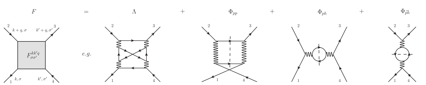
Figure 1: Two-particle vertex function $F$ (left) and its diagrammatic parquet decomposition (right), exemplified by the corresponding lowest order diagrams beyond the bare $U$. The (two-particle) cutting procedure indicating the two-particle reducibility of the last three terms is shown by the dashed lines.

The scheme of the paper is the following. In Sec. II we present the formalism relating the vertex function to generalized two-particle response functions as well as the parquet decomposition of the vertex function. We also briefly describe the model and the calculation method. In Sec. III we show results from the parquet decomposition and its behavior for intermediate and large $U$. In Sec. IV the behavior of the generalized susceptibility is discussed, and the origin of singularities in the generalized charge response function is shown. In Sec. V we discuss the relation of these singularities to the RVB character of the system, the pseudogap and the suppression of charge fluctuations. Sec. VI is devoted to our conclusions.

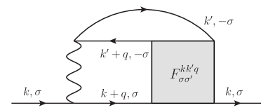
Figure 2: Diagrammatic representation of the self-energy $\Sigma$ in terms of the two-particle vertex function (Schwinger-Dyson equation of motion).

II Formalism, model and method

We first discuss the vertex function, following the notations of Rohringer et al.Rohringer2012 and Gunnarsson et al.FluctDiag We introduce the generalized susceptibility for finite temperature $T=1/\beta$, using the Matsubara formalism

$$\chi_{\sigma\sigma^{\prime}}(k;k^{\prime};q)=\int_{0}^{\beta}d\tau_{1}\int_{0}^{\beta}d\tau_{2}\int_{0}^{\beta}d\tau_{3}$$

$$\times e^{-i[\nu\tau_{1}-(\omega+\nu)\tau_{2}+(\omega+\nu^{\prime})\tau_{3}]}$$ (1)

$$\times\langle T_{\tau}[c^{\dagger}_{{\bf k}\sigma}(\tau_{1})c_{{\bf k}+{\bf q}\sigma}(\tau_{2})c^{\dagger}_{{\bf k}^{\prime}+{\bf q}\sigma^{\prime}}(\tau_{3})c_{{\bf k}^{\prime}\sigma^{\prime}}]\rangle$$

$$-\beta\,g_{\sigma}(k)g_{\sigma^{\prime}}(k^{\prime})\,\delta_{q=0}.$$

Here we use the condensed notations $q=({\bf Q},\omega)$ and $k=({\bf K},\nu)$, where ${\bf Q}$ and ${\bf K}$ are (cluster) wave vectors and $\omega$ and $\nu$ are Matsubara boson and fermion frequencies, respectively. We have also introduced a Green’s function $g_{\sigma}(k)\equiv g_{\sigma}({\bf K},\nu)$

$$g_{\sigma}(k)=-\int_{0}^{\beta}d\tau e^{i\nu\tau}\langle c_{{\bf K}\sigma}^{\phantom{\dagger}}(\tau)c_{{\bf K}\sigma}^{\dagger}\rangle,$$ (2)

where $c_{{\bf K}\sigma}^{\dagger}$ creates an electron with the wave vector ${\bf K}$ and spin $\sigma$ and $\langle..\rangle$ is the thermodynamical average. From $\chi$, and specifically from its connected part, we obtain the full two-particle vertex $F$:

$$\chi_{\sigma\sigma^{\prime}}(k;k^{\prime};q)=-\beta g_{\sigma}(k)g_{\sigma}(k+q)\delta_{kk^{\prime}}\delta_{\sigma\sigma^{\prime}}$$ (3)

$$-g_{\sigma}(k)g_{\sigma}(k+q)F_{\sigma\sigma^{\prime}}(k;k^{\prime};q)g_{\sigma^{\prime}}(k^{\prime})g_{\sigma^{\prime}}(k^{\prime}+q).$$

The vertex function $F$ is shown diagrammatically in Fig. 1, and it can be interpreted, physically, as the scattering rate amplitude between two added/removed electrons. Within the parquet formalism all diagrams contributing to $F$ are divided in two classes: Either they can be split in two parts by cutting two internal Green’s function lines (two particle reducibility: 2PR), or they cannot (two-particle irreducibility: 2PI) .

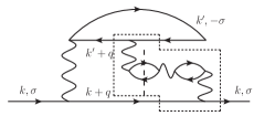
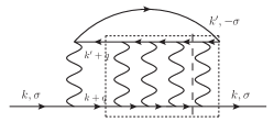
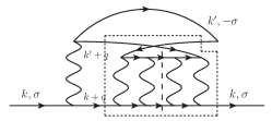
Figure 3: Examples of diagrams for the self-energy, with some explicit representations of the two-particle vertex function, enclosed by a dashed line. The dashed line shows how the vertex can be separated in two parts by cutting two Green’s functions. According to the rules in Sec. II, the diagrams are $ph$ (a), $\bar{ph}$ (b) and $pp$ (c) diagrams.

Moreover, because we are considering two-particle processes, whose diagrams have (altogether) four external lines, a finer classification can be performed for the 2PR diagrams. As exemplified by the diagrams on the right-hand side of Fig. 1, we can further distinguish among the cases, where, in the cutting-procedure, (i) lines 1 and 3 are separated from 2 and 4, which corresponds to particle-particle ($pp$) reducibility, (ii) lines 1 and 2 are separated from 3 and 4, i.e., longitudinal particle-hole ($ph$) reducibility, and, eventually, (iii) lines 1 and 4 are separated from lines 2 and 3, i.e. transverse particle-hole ($\bar{ph}$) reducibility. $F$ can then be written as a sum of these types of contribution

$$F=\Lambda+\Phi_{pp}+\Phi_{ph}+\Phi_{\bar{ph}},$$ (4)

where $\Lambda$ contains the pure 2PI contributions and the functions $\Phi$ describe the 2PR contributions in all different channels, as diagrammatically represented in Fig. 1: This is the parquet decomposition of the scattering amplitude $F$.

Finally, because of the electron spin, it is convenient to treat the $ph$ channel by introducing generalized charge ($ch$) and spin ($sp$) susceptibilities

$$\chi_{ch}(k;k^{\prime};q)=\chi_{\uparrow\uparrow}(k;k^{\prime};q)+\chi_{\uparrow\downarrow}(k;k^{\prime};q)$$ (5)

$$\chi_{sp}(k;k^{\prime};q)=\chi_{\uparrow\uparrow}(k;k^{\prime};q)-\chi_{\uparrow\downarrow}(k;k^{\prime};q)$$

We then define the quantities $\Gamma_{d}$ and $\Gamma_{m}$ which contain the diagrams of $F$ which are irreducible in the density and magnetic channels, respectively

$$\Gamma_{ch,sp}=\beta^{2}(\chi_{ch,sp}^{-1}-\chi_{0}^{-1}),$$ (6)

where $\chi_{0}$ is the generalized bare susceptibility, being a product of two interacting Green’s function. The $\chi$’s are treated as matrices in $k$ and $k$’ and $\Gamma$ can be calculated for one $q$ at a time. We also define the reducible quantities $\Phi_{ch,sp}$ via the Bethe-Salpeter equations

$$\Phi_{ch,sp}=F_{ch,sp}-\Gamma_{ch,sp}$$ (7)

$$\Phi_{ph\uparrow\downarrow}=F_{\uparrow\downarrow}-{1\over 2}(\Gamma_{ch}-\Gamma_{sp}),$$

and the parquet equationsRohringer2012 :

$$\Lambda_{\uparrow\downarrow}(k,k^{\prime},q)={1\over 2}[\Gamma_{ch}(k,k^{\prime},q)-\Gamma_{sp}(k,k^{\prime},q)]$$

$$+\Phi_{sp}(k,k+q,k^{\prime}-k)-\Phi_{pp}(k,k^{\prime},k+k^{\prime}+q)$$ (8)

By using the (Schwinger-Dyson) equation of motion, the electronic self-energy $\Sigma$ can be expressed in terms of two-particle vertex function:

$$\Sigma(k)-{Un\over 2}$$ (9)

$$=-{U\over\beta^{2}N_{c}}\sum_{k^{\prime},q}F_{\uparrow\downarrow}(k,k^{\prime},q)g(k^{\prime})g(k^{\prime}+q)g(k+q)$$

where $g=g_{\uparrow}=g_{\downarrow}$ (because of SU(2)-symmetry), $N_{c}$ is the number of ${\bf K}$-points. This is shown schematically in Fig. 2.

The equation of motion for $\Sigma$ is a well-known, general relation of many-body theory with a two-particle interaction. However, valuable information may be obtained by inserting in Eq. (9) the parquet decomposition of Eq. (4) and, in particular, its specific expression for $F_{\uparrow\downarrow}(k,k^{\prime},q)$:

$$F_{\uparrow\downarrow}(k,k^{\prime}\!,q)\!=\!\Lambda_{\uparrow\downarrow}(k,k^{\prime}\!,q)\!+\!\Phi_{pp,\uparrow\downarrow}(k,k^{\prime},k\!+\!k^{\prime}\!+\!q)$$ (10)

$$+\frac{1}{2}\Phi_{ch}(k,k^{\prime},q)-\frac{1}{2}\Phi_{sp}(k,k^{\prime},q)-\Phi_{sp}(k,k+q,k^{\prime}-k)$$

This way, after all internal summations are performed, the expression for $\Sigma$ is naturally split in four terms:

$$\Sigma=\tilde{\Sigma}_{\Lambda}+\tilde{\Sigma}_{pp}+\tilde{\Sigma}_{ch}+\tilde{\Sigma}_{sp}$$ (11)

evidently matching the corresponding 2PI and 2PR terms of Eq. (10): This represents the parquet decomposition of the self-energy. In fact, the four terms in Eq. 11 describe the contribution of the different channels (pp, charge, spin), as well as of the 2PI scattering processes, to the self-energy. Since each scattering channel is associated with definite physical processes, Eq. (11) can be exploited, in principle, for gaining a better understanding of the physics underlying a given self-energy calculation.

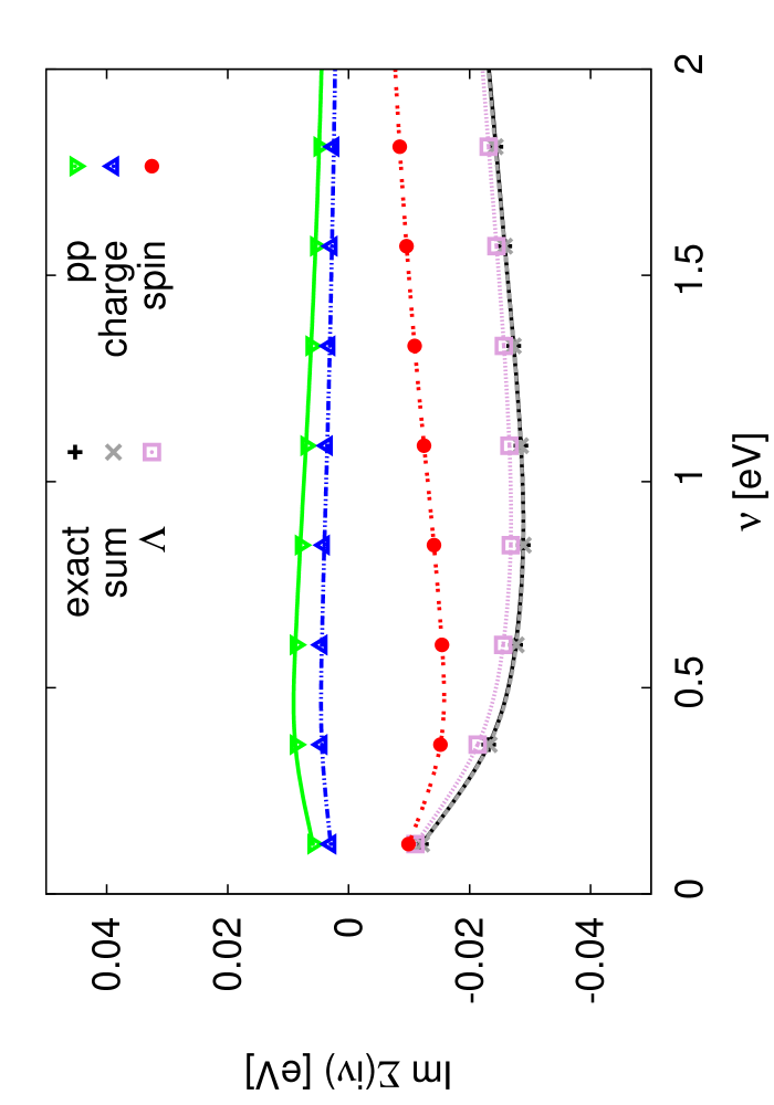
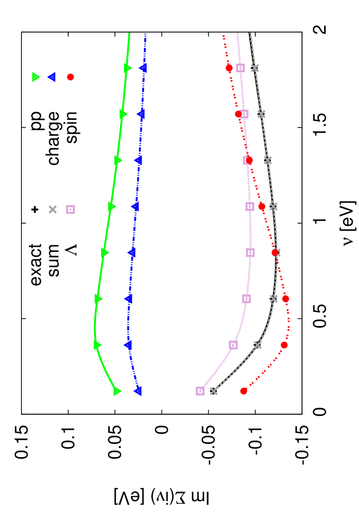
Figure 4: (Color online) Parquet decomposition of the DMFT self-energy $\Sigma(\nu)$ of the $3d$ Hubbard model at half-filling ($n=1$). The full (black, ”exact”) and dashed (gray, ”sum”) lines show $\Sigma$ as computed in DMFT, and as the sum of the parquet contributions, respectively. The colored symbols display the different contributions to $\Sigma(\nu)$ according to Eq. (11). The parameters of the calculation are: $N_{c}=1$ (DMFT), $t=-\frac{1}{2\sqrt{6}}\simeq-0.204$ eV, $\beta=26$ eV^-1 with two different values of the Hubbard interaction: $U=0.5$ eV (left panel), $U=1$ eV (right panel).

In the following section, we will apply this idea to specific cases of interest. In particular, we will test the performance of a parquet decomposition of the self-energy in the case of the three and two-dimensional Hubbard model on a simple cubic/square lattice, whose Hamiltonian reads

$$H=t\sum_{ij,\sigma}(c^{\dagger}_{i\sigma}c^{\phantom{\dagger}}_{j\sigma}+c^{\dagger}_{j\sigma}c^{\phantom{\dagger}}_{i\sigma})+U\sum_{i}n_{i\uparrow}n_{i\downarrow},$$ (12)

where $n_{i\sigma}=c^{\dagger}_{i\sigma}c^{\phantom{\dagger}}_{i\sigma}$, $t$ the hopping integral and $U$ is the on-site Coulomb interaction. For the sake of definiteness, $t=-0.25$ eV for the $2d$ case, and $t=-\frac{1}{2\sqrt{6}}\simeq-0.204$ eV for the 3d case. This choice ensures that the standard deviation ($D$) of the non-interacting DOS of the square and the cubic lattices considered is exactly the same ($D=1$eV), and thus allows for a direct comparison of the $U$ values used in the two-cases, provided they are expressed in units of $D$.

This Hamiltonian constitutes an important testbed case for applying the idea of a parquet decomposition, since Eq. (12) provides a quintessential representation of a strongly correlated system. Moreover, in the 2d case Eq. (12) is frequently adopted, e.g., to study the still controversial physics of cuprate superconductors.Dagotto ; Scalapino In this framework, we note that typical values for $U$ are about $U=8|t|=2$eV, i.e., $U$ is equal to the non-interacting bandwidth $W=8|t|$. This choice corresponds to a rather strong correlation regime, as it is clearly seen even in a purely DMFT context.Toschi2005 In this work, however, we will also consider smaller values of $U$, of the order of half bandwidth, corresponding to a regime of more moderate correlations.

III Parquet decomposition calculations

In this section we study the parquet decomposition of an electron self-energy computed by DMFT and DCA. In these non-perturbative methods a cluster with $N_{c}$ sites is embedded in a self-consistent electronic bath. The calculation of a generalized susceptibility is rather time-consuming when compared against computing only single-particle quantities. For this reason we restrict our calculations to the tractable values of $N_{c}=1$ (DMFT), $4$ and $8$ (DCA). The results are therefore not fully converged with respect to $N_{c}$, but, nevertheless, will illustrate well the specific points we make in the following sections. The cluster problem has been solved using both Hirsch-FyeHirschFye and continuous time (CT)CT methods.

Consistent with the discussion of the previous section, we will use Eq. (9), illustrated diagrammatically in Fig. 2, and Eqs. (4), (10) to express the self-energy in terms of contributions from the different parquet channels. As for the latter, in Fig. 3 we show some typical diagrams, and their classifications according to the parquet decomposition. Using the definitions in Sec. II, Fig. 3a and b show longitudinal and transverse particle-hole reducible diagrams, respectively, and Fig. 3c shows a particle-particle reducible diagram. In fact, the vertex diagram in Fig. 3a contains contributions to the random phase approximation for the longitudinal charge and spin susceptibilities, reducible in spin- and charge-channel. In the same way, the diagram in Fig. 3b contains a contribution to the transverse spin susceptibility and Fig. 3c displays a particle-particle ladder diagram.

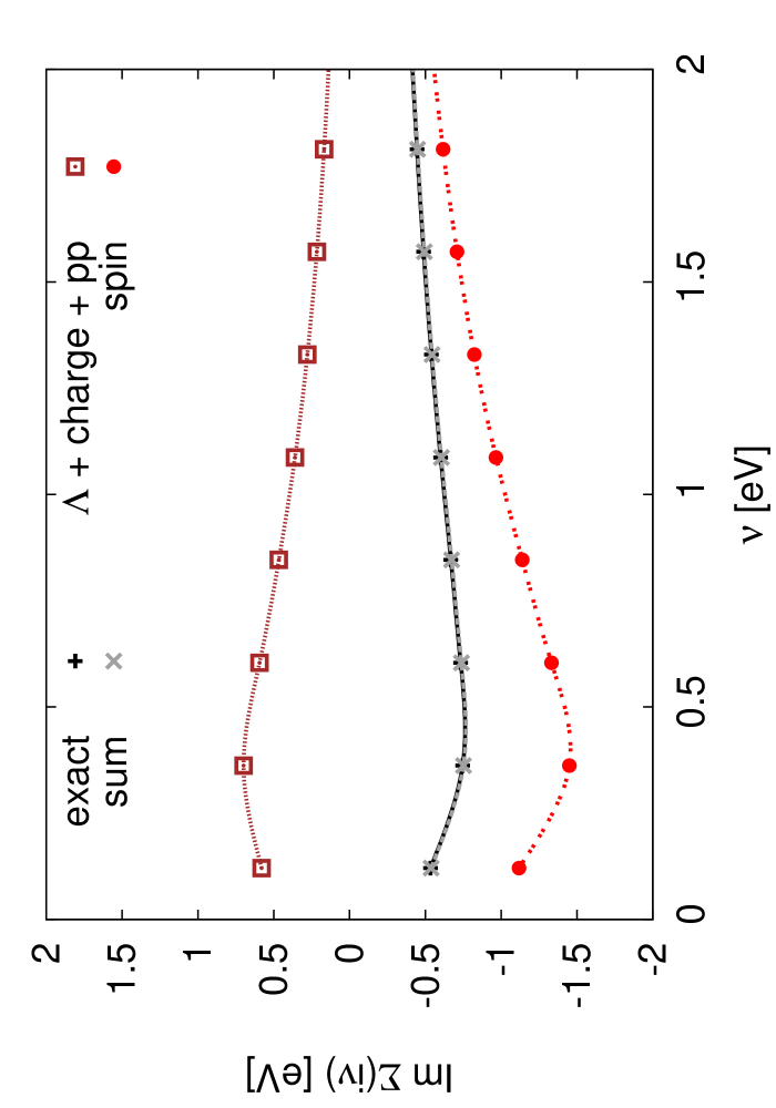
Figure 5: (Color online) left panel: Parquet decomposition of the DMFT self-energy $\Sigma(\nu)$ as in Fig. 4, but with $U=2$ eV. Right panel: Bethe-Salpeter decomposition in the spin channel of the same DMFT self-energy.

III.1 DMFT results

We start by applying the parquet decomposition to the easier case of the DMFT self-energy. In particular, we will focus on one of the most studied cases in DMFT, the half-filled Hubbard model in $3d$, where DMFT describes a Mott-Hubbard metal-insulator transition at a finite $U=U_{MIT}$. The specific parameters in Eq. (12) have been chosen in this case as follows: $n=1$ (half-filling) and $\beta=26$ eV^-1. The results of the parquet decomposition of the DMFT self-energy are shown in Fig. 4 in the weak-to-intermediate coupling regime $U\ll{U_{MIT}}\sim 3$ eV. The plots show the imaginary part of the DMFT self-energy (solid black line) as a function of the Matsubara frequencies i$\nu$ and for two different values of $U$ (we recall that $\Sigma$ does not depend on momentum in DMFT, and that in a particle-hole symmetric case, as the one we consider here, it does not have any real part beyond the constant Hartree term).

By computing the DMFT generalized local ($N_{c}=1$) susceptibility of the associated impurity problem, and proceeding as described in the previous section, we could actually decompose Im $\Sigma(i\nu)$ into the four contributions from terms in Eq. (11), depicted by different colors/symbols in the plots. Before analyzing their specific behaviors, we note that their sum (gray dashed line) does reproduce precisely the value of Im $\Sigma$ directly computed in the DMFT algorithm. Since all the four terms of Eq. 11 are calculated independently from the parquet-decomposed equation of motion, this result represents indeed a stringent test of the numerical stability and the algorithmic correctness of our parquet decomposition procedure. Given the number of steps involved in the algorithm, illustrated in the previous section, the fulfillment of such a self-consistency test is particularly significant, and, indeed, it has been verified for all the parquet decomposition calculations presented in this work.

By considering the most weak-coupling data first ($U=0.5$eV, left panel of Fig. 4), we note that the 2PI contribution ($\Sigma_{\Lambda}$ in Eq. (11), plum-colored open squares in the Figure) lies almost on top of the “exact” DMFT self-energy. At weak-coupling this is not particularly surprising, because $\Lambda_{\uparrow\downarrow}\simeq U+O(U^{4})$, while all the 2PR contributions are at least $O(U^{2})$. Hence, when the 2PI vertex is inserted into the equation of motion, $\tilde{\Sigma}_{\Lambda}$ simply reduces to the usual second-order perturbative diagram. In this situation (i.e., Im $\Sigma(i\nu)\simeq\tilde{\Sigma}_{\Lambda}$), it is interesting to observe that the other sub-leading contributions (spin, particle-particle scattering and charge channel) are not fully negligible. Rather, they almost exactly compensate each other: the extra increase of the scattering rate [i.e.: -Im $\Sigma(i\nu\rightarrow 0)$] due to the spin-channel is compensated (or “screened”) almost perfectly by the charge- and the particle-particle channel.

Not surprisingly, the validity of this cancellation is gradually lost by increasing $U$. At $U=1.0$ (right panel of Fig. 4), which is still much lower than $U_{MIT}$, one observes that the 2PI contribution no longer provides so accurate values for Im $\Sigma(\nu)$. At the same time, the contributions of all scattering channels increase: the low-frequency behavior of the spin channel now would provide -taken on its own- a scattering rate even larger than the true one of DMFT. Consistently, a correspondingly larger compensation of the charge and the particle-scattering channels contribution is observed. At higher frequency, these changes w.r.t. the previous case are mitigated, matching the intrinsic perturbative nature of the high-frequency/high-T expansionsKunes2011 ; Georgthesis ; Stefanthesis .

The situation described above, which suggests an important role of spin fluctuations, partially screened by charge and particle-particle scattering processes, displays important changes at intermediate-to-strong coupling $U$. This is well exemplified by the data reported in Fig. 5 (left panel). Despite the DMFT self-energy still displays a low-frequency metallic bending ($U=2.0$ is on the metallic side of the DMFT MIT), in the low-frequency region one observes the appearance of a huge oscillatory behavior in the parquet decomposition of $\Sigma$: All contributions to Im $\Sigma$, but the spin term (s. below), are way larger than the self-energy itself and fluctuate so strongly in frequency, that several changes of sign are observed. This makes it obviously very hard to define any kind of hierarchy for the impact of the corresponding scattering channels on the final self-energy result.

Hence, at these intermediate-to-strong values of $U$ the parquet decomposition procedure appears to be no longer able to fully disentangle the physics underlying a given (here: DMFT) self-energy. At the same time, we should stress that the strong oscillations visible in the parquet decomposition of Fig. 5 can not be ascribed to numerical accuracy issues. In fact, one observes, that, also in this problematic case, the self-consistency test works as well as for the other data sets: the total sum of such oscillating contributions, still reproduces the Im $\Sigma(\nu)$ from DMFT in the whole frequency range considered. The reason of such behavior has to be traced back, instead, to the divergencies of the 2PI vertices recently reported in DMFT work.divergence ; Georgthesis ; Schaeferthesis ; Janis2014 ; Kozik2015 While the relation with such divergencies will be extensively discussed in Sec. IV, it is worth stressing already here, that there is only one contribution to $\Sigma(\nu)$, which never displays wild oscillation, even for intermediate-to-strong $U$: the spin channel. This means that even when the parquet decomposition displays a strong oscillatory behavior, a Bethe-Salpeter decomposition in this specific (spin) channel will always remain well-behaved and meaningful. This is explicitly shown in Fig. 5 (right panel), where all the contributions to $\Sigma(\nu)$, but $\tilde{\Sigma}_{sp}$, (i.e., formally: all the contributions 2PI in the spin channel) are summed together: Here no oscillation is visible. The results of such Bethe-Salpeter decomposition of $\Sigma(\nu)$ in the spin channel suggests then again an interpretation of a physics dominated by this scattering channel, though -this time- in the non-perturbative regime: Strong (local) spin fluctuations, originated by the progressive formation of localized magnetic moments, are responsible for the major part of the electronic self-energy and scattering rate. Their effect is, as before, partly reduced, or screened, by the scattering processes in the other channels (opposite sign contribution to Im $\Sigma$). Differently as before, however, the specific role of the “secondary” channels can no longer be disentangled via our parquet decomposition.

III.2 DCA results

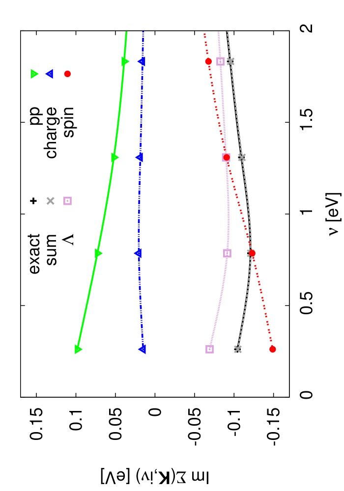
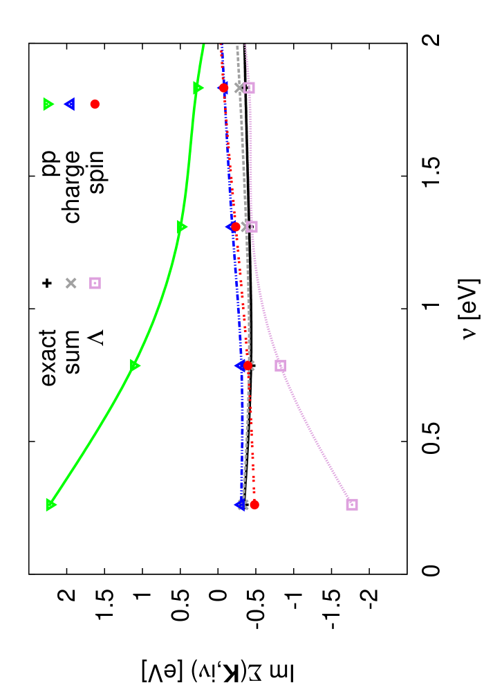
Figure 6: (Color online) Parquet decomposition of the DCA self-energy $\Sigma[{\bf K}=(\pi,0),\nu]$. The same convention of Fig. 4 is adopted. The parameters of the calculations are $N_{c}=8$, $t=-0.25$ eV, $\beta=12$ eV^-1 and the filling is $n=0.85$ with two different values of the Hubbard interaction: $U=1.0$ eV (left panel), $U=2.0$ eV (right panel)

In this subsection, we discuss the numerical results for the parquet decomposition of self-energy data computed in DCA. Different from DMFT, the DCA self-energy provides a more accurate description of finite dimensional systems, as it is also explicitly dependent on the momenta of the discretized Brillouin zone (i.e., a cluster of $N_{c}$ patches in momentum space) of the DCA. We will present here parquet decomposition results for the self-energy of the two-dimensional Hubbard model with hopping parameter $t=-0.25$ for different values of the density $n$ and of the interaction $U$. In particular, we will mostly focus on the self-energy at the so called anti-nodal point, ${\bf K}=(\pi,0)$, because it usually displays the strongest correlation effects for this model and also because the vector ${\bf K}=(\pi,0)$ is always present in both clusters we used ($N_{c}=4,8$) in our DCA calculation. We note, however, that the results of the parquet decomposition for the other relevant momenta of this system, i.e. the nodal one ${\bf K}=(\pi/2,\pi/2)$, (for $N_{c}=8$ where it is available), are qualitatively similar.

As for the DMFT case, we start by considering a couple of significant cases at fixed density (here $n=0.85$, corresponding to the typical $15$% of hole doping of the optimally doped high-T_c cuprates), and perform the parquet decomposition for different $U$. In the left panel of Fig. 6 we show the calculations performed at a moderate $U=4|t|=1$eV (interaction equal to the semibandwidth). As one sees the results are qualitatively similar to the DMFT one at intermediate coupling (right panel of Fig. 4), which one could indeed interpret in terms of predominant spin-scattering processes, partially screened by the other channels. However, also in DCA, extracting such information from the parquet decomposition becomes rather problematic for larger values of $U$. At $U=8|t|=2$ eV (interaction equal to the bandwidth: Fig. 6 right panel), the parquet decomposition appears dominated by contributions from the 2PI and the $pp$ channel: These become an order of magnitude larger than the spin-channel contribution and of the total DCA self-energy. This finding, in turn, indicates the occurrence of large cancellation effects in the parquet-decomposed basis, making quite hard any further physical interpretation.

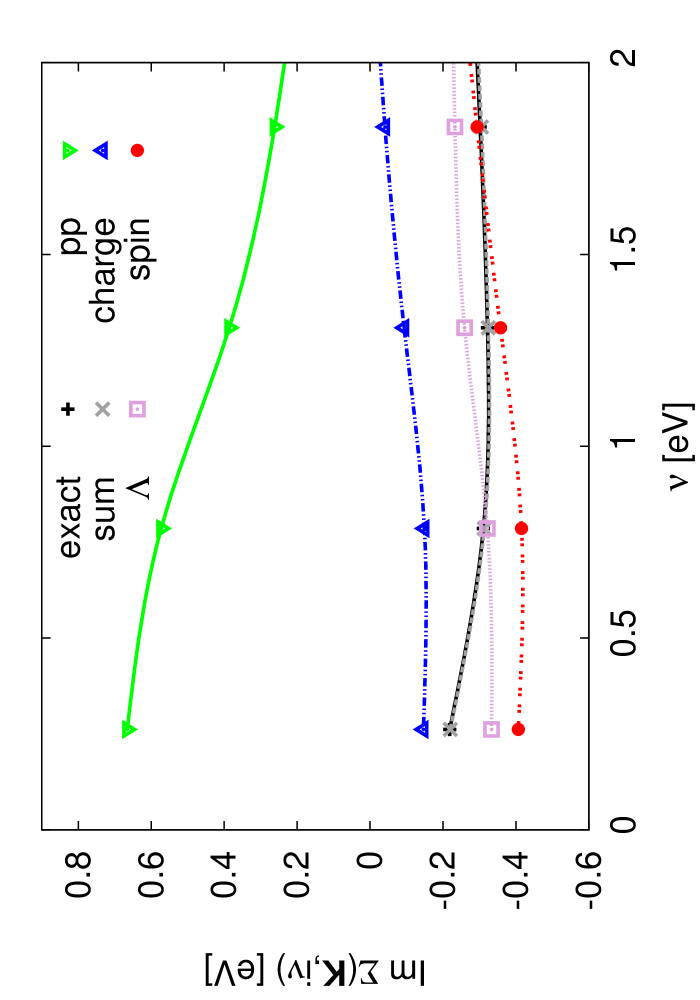
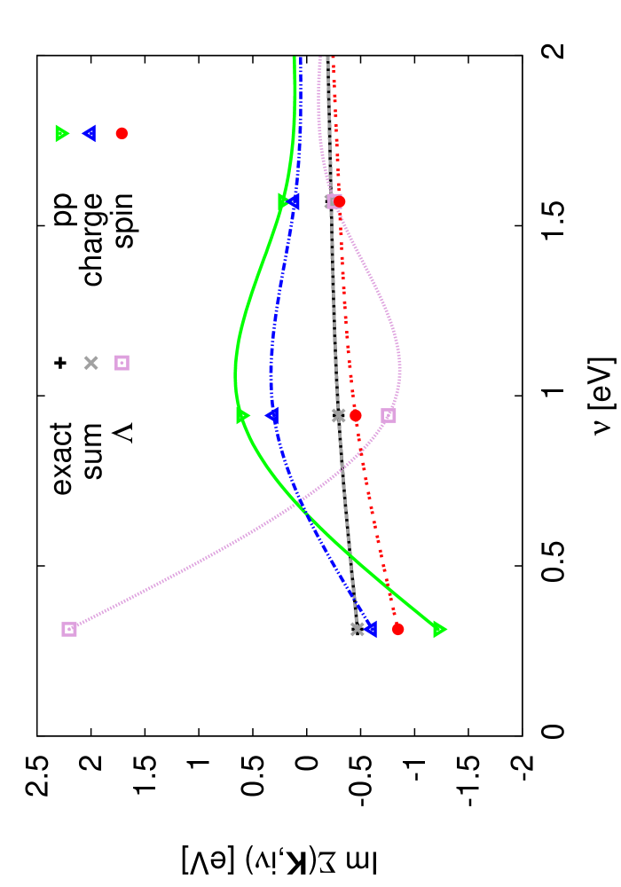
Figure 7: Parquet decomposition of the DCA self-energy $\Sigma[{\bf K}=(\pi,0),i\nu]$ ($N_{c}=8)$ at different dopings. Left panel: high hole doped case ($n=0.75$) for the same interaction/temperature values as in right panel of Fig. 6 ($U=2$ eV and $\beta=12$ eV^-1). Right panel: undoped case ($n=1$), at intermediate-to-strong coupling ($U=1.4$ eV and $\beta=10$ eV^-1, calculated for a $N_{c}=4$ DCA cluster.

It is also instructive to look at the effect of a change in the level of hole-doping on the parquet decomposition calculations. This is done in Fig. 7: In the left panel of the figure results for the highly doped case $n=0.75$ ($25$% hole doping) are shown. Despite the large value of the interaction $U=2$ eV, this parquet decomposition looks qualitatively similar to the one at moderate coupling of the less doped case Fig. 6 (left panel). Conversely, at half-filling ($n=1$, right panel of Fig. 7), although we chose a lower value of $U=1.4$ eV, the parquet decomposition displays the very same large oscillations among different channel contributions observed in the DMFT data (Fig. 5, left panel). Hence, our parquet decomposition procedure applied to the DCA results allows us to extend the considerations drawn from the DMFT analysis of the previous section: For a large enough value of $U$ and moderate or no doping, the parquet decomposition of the self-energy becomes rather problematic, as some channel contributions (supposed to be secondary) become abruptly quite large, or even strongly oscillating, with large cancellation between different terms. The inclusion of non-local correlations within the DCA allows us to demonstrate that this is not a special aspect of the peculiar, purely local, DMFT physics, but it survives also in presence of non-local correlations. Actually, as we will discuss in the next sections, the non-local correlations do favor the occurrence of singularities in the parquet decomposition, which is observed for DCA in a correspondingly larger parameter region (at lower $U$ and hole-doping) than in DMFT.

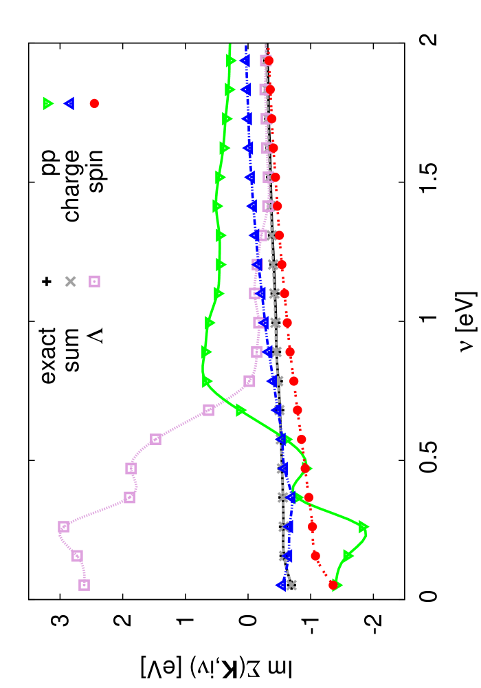
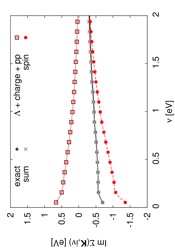
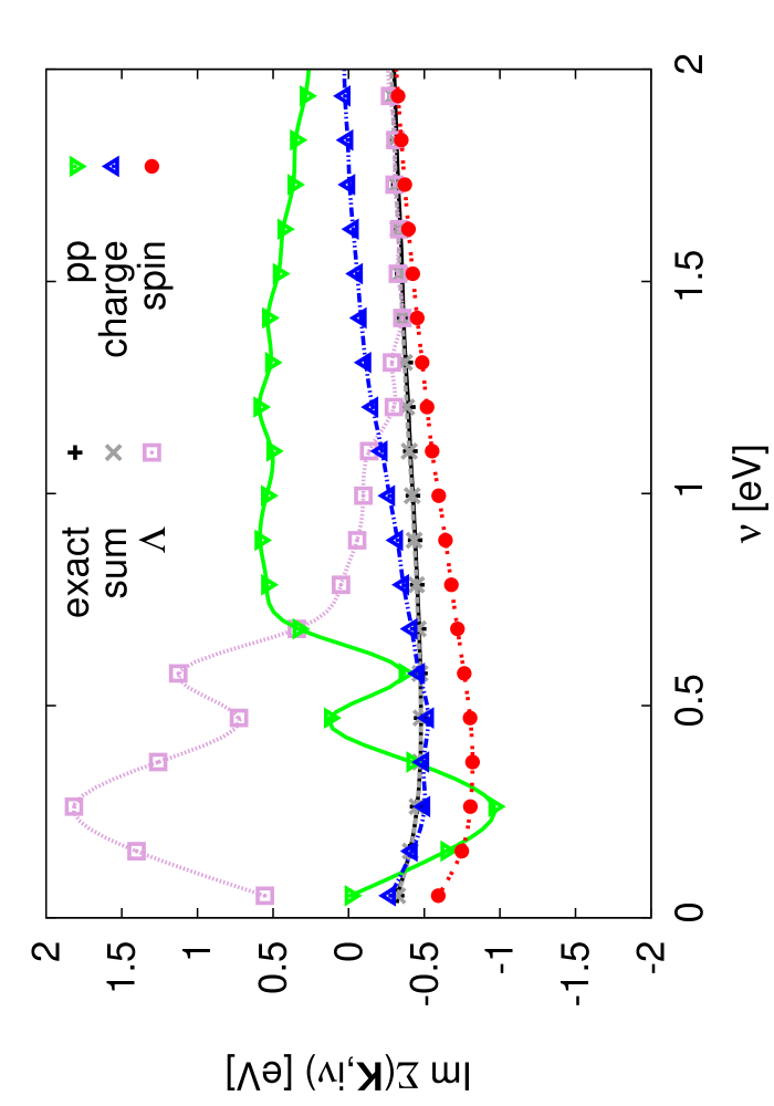
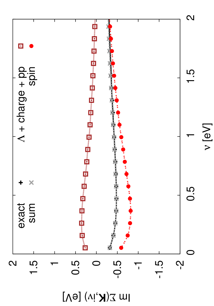
Figure 8: Parquet decomposition of the DCA self-energy $\Sigma[{\bf K},i\nu]$ with $N_{c}=8$ for the low-$T$, underdoped case $n=0.94$ with $U=1.75$ eV and $\beta=60$ eV^-1 (see text). Left upper panel: parquet decomposition for the antinodal DCA self-energy [${\bf K}=(\pi,0)$]; right upper panel: Bethe-Salpeter decomposition of the antinodal DCA self-energy. Left lower panel: parquet decomposition of the nodal[${\bf K}=(\frac{\pi}{2},\frac{\pi}{2})$] DCA self-energy. Right lower panel: Bethe-Salpeter decomposition of the nodal DCA self-energy.

In this perspective, it is interesting to investigate, whether the singularities in the parquet decomposition, with their intrinsically non-perturbative nature, already occur in a parameter region where the DCA self-energy displays a strong momentum differentiation, with pseudogap features. As discussed in Ref. FluctDiag, , such a case is achieved in a $N_{c}=8$ DCA calculation for, e.g.,: $n=0.94$ ($6$% hole doping), $U=1.75$ eV, $\beta=60$ eV${}^{-}1$ (with the additional inclusion of a realistic next-to-nearest hopping term $t^{\prime}=0.0375$ eV). In the left panels of the Fig. 8 the DCA self-energy for the anti-nodal and the nodal momentum is shown, together with its corresponding parquet decomposition. We note, as it was also stated in Ref. FluctDiag, , that the positive (i.e., non Fermi-liquid) slope of Im$\Sigma({\bf K},i\nu)$ in the lowest frequency region for $\mathbf{K}=(\pi,0)$ indicates a pseudogap spectral weight suppression at the antinode. The parquet decomposition of the two self-energies is, however, very similar: The strong oscillations of the various channels clearly demonstrate that in the parameter region where a pseudogap behavior is found in DCA, the parquet decomposition displays already strong oscillations. It is also interesting to notice that, similarly as we discussed in the previous section, also in this case, the spin channel contribution of the parquet decomposition is the only one displaying a well-behaved shape, with values of the order of the self-energy and no frequency oscillations. Consequently, also for the DCA self-energy in the pseudogap regime, a Bethe-Salpeter decomposition in the spin-channel of the self-energy remains valid (see right panel of Fig. 8). As discussed in the previous section, this might be interpreted as an hallmark of the predominance of the spin-scattering processes in a non-perturbative regime, where a well-behaved parquet decomposition is no longer possible. In this perspective, the physical interpretation would match very well the conclusions derived about the origin for the pseudogap self-energy of DCA by means of the recently introduced fluctuation diagnostics methodFluctDiag . At present, hence, the post processing of a given numerical self-energy provided by the fluctuation diagnostics procedure appear the most performant, because -differently from the parquet decomposition- it remains applicable, without any change, also to non-perturbative cases.

After discussing our parquet decomposition calculations, their proposed physical interpretation, and their limitation in applicability, it is natural to wonder, where such limitations arise from. This analysis is, in fact, very important also beyond the calculations presented in this work, because the parquet equations represent the base-camp of several novel quantum many body schemes aiming at the the description of strongly correlated electron beyond the perturbative regime.

As we anticipated before, the reason for the occurrence of strong low-frequency oscillations in the parquet decomposition can be traced to the divergence of the 2PI irreducible vertex functions observed by increasing $U$,divergence or -equivalently- to the occurrence of singularities in the generalized $ph$ charge ($\chi_{ch}$) and $pp$ ($\uparrow\downarrow$ and/or singlet) ($\chi_{pp}$) susceptibilities. The investigation of the exact relation between the peculiar behavior of the parquet decomposition by increasing $U$ and the singularities of the corresponding generalized susceptibility matrix will be explicitly addressed below.

IV Singularities of generalized susceptibilities

In this section, we aim at clarifying why some contributions of the parquet decomposition start displaying singularities and strong oscillatory behaviors upon increasing $U$. From a general perspective, since the singularities observed in the previous section always affect $\tilde{\Sigma}_{\Lambda}$, the contribution stemming from the 2PI vertex, a clear relation must exist with corresponding divergencies of the 2PI vertices. In fact, the occurrence of divergences in the 2PI vertices of the Hubbard and Falicov-Kimball model has been recently demonstrated by means of analytic and DMFT calculations.divergence ; Janis2014 In particular, we recall that such singularities show up simultaneously in the fully 2PI vertex $\Lambda$ as well as in the irreducible vertices $\Gamma_{r}$ in the charge ($r=ch$) and particle-particle channel($r=pp,\uparrow\downarrow$), while the full vertex $F$ and the self-energy remain always well-behaved. Evidently, this perfectly matches the problematic channels of our parquet decompositions.

As discussed in Ref. [divergence, ], a divergence of a $\Gamma_{r}$ must be associated to a non-invertibility of its corresponding Bethe-Salpeter equation and, hence, according to Eq. (6), to the occurrence of singular ($=0$) eigenvalue in the generalized susceptibility matrix $\chi_{r}(k;k^{\prime};q)$. In fact, when an eigenvalue goes through zero, the irreducible vertex functions change qualitatively. In particular, one observes that second order perturbation theory breaks down, failing to reproduce even the sign of the vertex-functions at low frequencies. In this sense the system is then in the truly strong-coupling limit. In Ref. divergence, , $\chi_{ch}(k;k^{\prime};q)$ was computed in DMFT ($N_{c}=1$), treating $\chi_{ch}$ as a matrix in $k$ and $k^{\prime}$ for fixed $q$. For the case when the frequency transfer $\omega$ is zero, we showed that the lowest eigenvalue of this matrix becomes negative as $U$ is increased. A similar behavior was found for $\chi_{pp}$ in the $\uparrow\downarrow$ sector (or in the singlet channel) for a somewhat larger $U$.

In the following, we will analyze in more details such divergencies, by extending the previous DMFT ($N_{c}=1$) resultsdivergence to DCA ($N_{c}=4$), and by investigating in details how singularities develop in the generalized susceptibility matrices and how they affect the parquet decompositions of the self-energy.

IV.1 $N_{c}=1$ case

For the sake of clarity we start by analyzing the generalized charge susceptibility in the $N_{c}=1$ (DMFT) case, focusing on the most-correlated case of half-filling. In particular we will mainly study the most singular case of $\omega=0$. In fact, $\omega=0$ represents the largest contribution to the parquet decomposition for the values of $T$ studied here, and, thus, its behavior is particularly significant. The case $\omega\neq 0$, nonetheless, will be also discussed briefly afterwards.

For a very small value of $U$, where no problem in the parquet decomposition is observed, we can approximate the generalized charge susceptibility with the non interacting one, i.e., with a product of two Green’s functions $\chi_{ch}(\nu,\nu^{\prime},\omega=0)\simeq\chi^{0}(\nu,\nu^{\prime},\omega=0)\delta_{\nu,\nu^{\prime}}$. In addition we can use noninteracting Green’s functions. The corresponding diagonal elements are given by

$$\chi_{ch}(\nu;\nu;\omega=0)\simeq-{\beta\over N_{k}^{2}}\sum_{{\bf k},{\bf k}^{\prime}}{1\over(i\nu+\mu-\varepsilon_{\bf k})(i\nu+\mu-\varepsilon_{{\bf k}^{\prime}})},$$ (13)

where $N_{k}$ is the number of ${\bf k}$-points and $\varepsilon_{\bf k}$ is the corresponding single-particle energy eigenvalue. Off-diagonal elements will obviously appear at finite $U$, remaining however much smaller than the diagonal ones in the perturbative regime. If we now consider the limit of very large $\nu$, the diagonal elements behave as $\beta/\nu^{2}$ and, hence, also become very small. In the numerical calculations, we limit the range of $|\nu|$ to some maximum value $\nu_{\rm max}$. Hence, in the perturbative regime, the lowest eigenvalue of $\chi_{ch}$ will correspond roughly to the value of the diagonal element for $\nu=\nu_{\rm max}$, and its eigenvector will have weight for $\nu=\pm\nu_{\rm max}$.

As $U$ is increased, however, the off-diagonal elements $\nu^{\prime}\neq\nu$ become gradually more important until, at a certain point, (e.g., at $U=\bar{U}\sim 1.27$ eV for the temperature we considered) this picture changes radically: The off-diagonal component of $\chi_{ch}(\nu,\nu^{\prime},\omega=0)$ for small frequencies become comparable or larger than the corresponding diagonal ones. As a consequence (see appendix B), the lowest eigenvalue of $\chi_{ch}(\nu,\nu^{\prime},\omega=0)$ crosses zero and, for large interaction, a negative eigenvalue appears. In contrast to the small $U$ case, the corresponding vector has most of its weight for $\nu=\pm\pi/\beta$: For these parameters the total weight of two elements for $\nu=\pm\pi/\beta$ is about $0.85$. This indicates that a crossing of energy levels has occurred between a lowest eigenvector having most of the weight at large frequencies to the one having most of the weight for small frequencies.notelowT

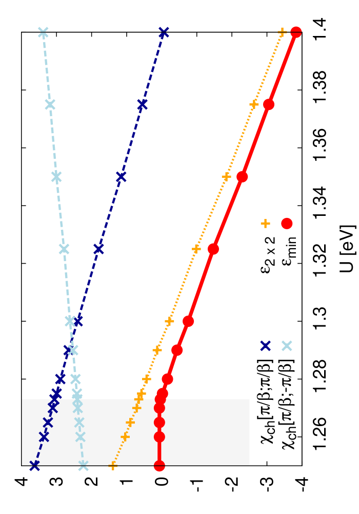
Figure 9: Plot of the lowest eigenvalue of $\chi_{ch}(\nu,\nu^{\prime},\omega=0)$ as a function of $U$. The parameters of the calculation are $t=-0.25$ eV, $\beta=10$ eV^-1, $n=1$, and $N_{c}=1$ (DMFT). The gray shadowed area marks the (perturbative) parameter region ($U<\bar{U}$), where the level-crossing of the lowest eigenvalue has not yet occurred (see text). The numerical values of $\varepsilon_{min}$ are then compared with the approximation in Eq. (14). Finally, the corresponding diagonal and off-diagonal elements of $\chi_{ch}$ for $\nu=\pm\pi/\beta$ are also plotted.

In this situation, the most significant piece of information can be extracted by restricting the analysis to the matrix elements for $\pm\pi/\beta$, i.e., to a $2\times 2$ matrix in frequency space. Then the lowest eigenvalue of $\chi_{ch}$ is

$$\varepsilon_{\rm 2\times 2}=\chi_{ch}({\pi\over\beta};{\pi\over\beta})-|\chi_{ch}({\pi\over\beta};-{\pi\over\beta})|.$$ (14)

This approximation is compared with the exact eigenvalue in Fig. 9. It provides a good approximation after the level crossing has occurred, i.e., where the lowest eigenvalue of $\chi_{ch}$ has become negative. Fig. 9 also shows the elements $\chi_{ch}(\pi/\beta;\pi/\beta)$ and $\chi_{ch}(\pi/\beta;-\pi/\beta)$. The diagonal element decreases and the off-diagonal element increases as $U$ is increased. Approximately as they cross, the lowest eigenvalue goes negative (the minor deviation of $\simeq 0.02$U reflects the corresponding small difference between $\varepsilon_{\rm 2\times 2}$ and $\varepsilon_{\rm min}$).

As the lowest eigenvalue $\varepsilon_{\rm min}$ of $\chi_{ch}(\nu,\nu^{\prime},\omega=0)$ goes through zero, $\chi_{ch}^{-1}$ becomes infinite. For the cases we have studied, the diagonal and off-diagonal matrix elements of the $2\times 2$ matrix have the same sign when this happens. Consequently, for the corresponding (singular) eigenvector, the elements for $\nu=\pm\pi/\beta$ then have opposite signs. It then follows from Eq. (24) that the diagonal and off-diagonal parts, $\chi_{ch}^{-1}(\pi/\beta;\pi/\beta)$ and $\chi_{ch}^{-1}(\pi/\beta;-\pi/\beta)$ also have opposite signs. Inserting $\chi_{ch}^{-1}$ in the expression needed for the parquet decomposition, we then find that a cancellation of the singular contributions does occur (see Appendix B).

However, as one can easily infer from the right side of Fig. 9), at larger values of $U$, the sign of the diagonal matrix element changes, and then the (now non-singular) contributions add constructively. Hence, when a second eigenvalue of $\chi_{ch}(\nu,\nu^{\prime},\omega=0)$ crosses zero, no cancellation will occur and the singularity will show up in the corresponding terms of the parquet decomposition of $\Sigma(i\nu)$.

In particular, from Ref. [divergence, ] we know that a second divergence takes place at a slightly larger value of $U$ than the range of Fig. 9. In particular, for $U>1.6$ eV, a second eigenvalue of $\chi_{ch}(\nu,\nu^{\prime},\omega=0)$ vanishes, simultaneously with the first one of $\chi_{pp,\uparrow\downarrow}(\nu,\nu^{\prime},\omega=0)$ As discussed above, now, the sign of the matrix elements is such that the singular contributions to the parquet decomposition no longer cancel. Then the parquet decomposition, in its corresponding counterparts ($\tilde{\Sigma}_{ch}$, $\tilde{\Sigma}_{pp}$ and -consequently- $\tilde{\Sigma}_{\Lambda}$), blows up at low-frequencies. Hence, for somewhat larger values of $U$ results similar to Figs. 5 are obtained. At the same time we find, consistent with the findings of Ref. [divergence, ], that no vanishing eigenvalue occurs in $\chi_{sp}(\nu,\nu^{\prime},\omega=0)$ even at larger $U$ and $\tilde{\Sigma}_{sp}$ remains well-behaved also at strong coupling.

A more physical elaboration of the meaning of such a selective appearance of singularities in the different channels will be given in the last section of the paper.

Until now we have discussed the case $\omega=0$. For $\omega\neq 0$ there are negative diagonal matrix elements of $\chi_{ch}$ even for small values of $U$. For instance, already in a generalization of Eq. (13) negative diagonal matrix elements can appear. These elements are particularly small for large $\nu$ and $\omega$. Hence, inverting such a matrix gives large matrix elements for large $\nu$ and $\omega$, which are rather unimportant for the self-energy and, thus, not very interesting in the light of the parquet decomposition.

IV.2 $N_{c}=4$ case

Table 1: Important matrix elements of $\chi_{d}({\bf K},\nu;{\bf K}^{\prime},\nu^{\prime};{\bf Q},\omega)$ for ${\bf Q}=(\pi,\pi)$ and $\omega=0$. The parameters are $N_{c}=4$, $t=-0.25$ eV, $U=1.5$ eV and $\beta=10$ eV^-1.

$\nu$	${\bf K}$	$\nu^{\prime}=-\pi/\beta$				$\nu^{\prime}=\pi/\beta$
		$(\pi,\pi)$	$(\pi,0)$	$(0,\pi)$	$(0,0)$	$(\pi,\pi)$	$(\pi,0)$	$(0,\pi)$	$(0,0)$
$-\pi/\beta$	$(\pi,\pi)$	7.4	-1.7	-1.7	-4.0	0.4	0.6	0.6	-0.0
$-\pi/\beta$	$(\pi,0)$	-1.7	4.8	-16.	-1.7	0.6	3.9	2.3	0.6
$-\pi/\beta$	$(0,\pi)$	-1.7	-16.	4.8	-1.7	0.6	2.3	3.9	0.6
$-\pi/\beta$	$(0,0)$	-3.9	-1.7	-1.7	7.4	0.0	0.6	0.6	0.4
$\pi/\beta$	$(\pi,\pi)$	0.4	0.6	0.6	0.0	7.4	-1.7	-1.7	-4.0
$\pi/\beta$	$(\pi,0)$	0.6	3.9	2.3	0.6	-1.7	4.8	-16.	-1.7
$\pi/\beta$	$(0,\pi)$	0.6	2.3	3.9	0.6	-1.7	-16.	4.8	-1.7
$\pi/\beta$	$(0,0)$	0.0	0.6	0.6	0.4	-3.9	-1.7	-1.7	7.4

We will now extend the previous DMFT analysis of the singularities to the DCA calculations for $N_{c}=4$.

In this case, $\chi_{ch}$ is also momentum dependent, and, in general, a complex function. However, at half-filling, for ${\bf Q}=(\pi,\pi)$ and $\omega=0$ it remains purely real.noteotherQ We therefore mostly focus on this case, which gives an important contribution to $\Sigma$. As in the previous section, we use the parameters $t=-0.25$ eV and $\beta=10$ eV^-1, and study the occurrence of vanishing eigenvalues in $\chi_{ch}$.

Since, as discussed at the beginning of last section, we are not interested in the high-frequency (perturbative) eigenvalues of $\chi_{ch}$, we choose an interaction value, where the most important fermion frequencies have already become the lowest ones: $\nu,\nu^{\prime}=\pm\pi/\beta$. In particular, Table 1 shows some of these matrix elements for, e.g., $U=1.5$ eV. Here, one sees that the dominating off-diagonal matrix elements are obtained for $\nu=\nu^{\prime}=\pm\pi/\beta$ and ${\bf K}\neq{\bf K}^{\prime}$ taking values $(\pi,0)$ or $(0,\pi)$. Based on the size of the different matrix elements in Table 1, it is then natural to focus on the $4\times 4$ matrix containing the ${\bf K}$-vectors $(\pi,0)$ and $(0,\pi)$ as well as the frequencies $\nu,\nu^{\prime}=\pm\pi/\beta$ for ${\bf Q}=(\pi,\pi)$ and $\omega=0$. The lowest eigenvalue of this matrix is defined as $\varepsilon_{4\times 4}$. We also calculate the lowest eigenvalue, $\varepsilon_{{\bf K}\times{\bf K}}$, corresponding to the the $2\times 2$ matrix containing the two ${\bf K}$-vectors at the Fermi-level, $(\pi,0)$ and $(0,\pi)$, for one frequency, i.e., $\nu=\pi/\beta$. Finally, we calculate the lowest eigenvalue, $\varepsilon_{\nu\times\nu}$ corresponding to the $2\times 2$ matrix containing two frequencies $\nu,\nu^{\prime}=\pm\pi/\beta$ and one ${\bf K}=(\pi,0)$.

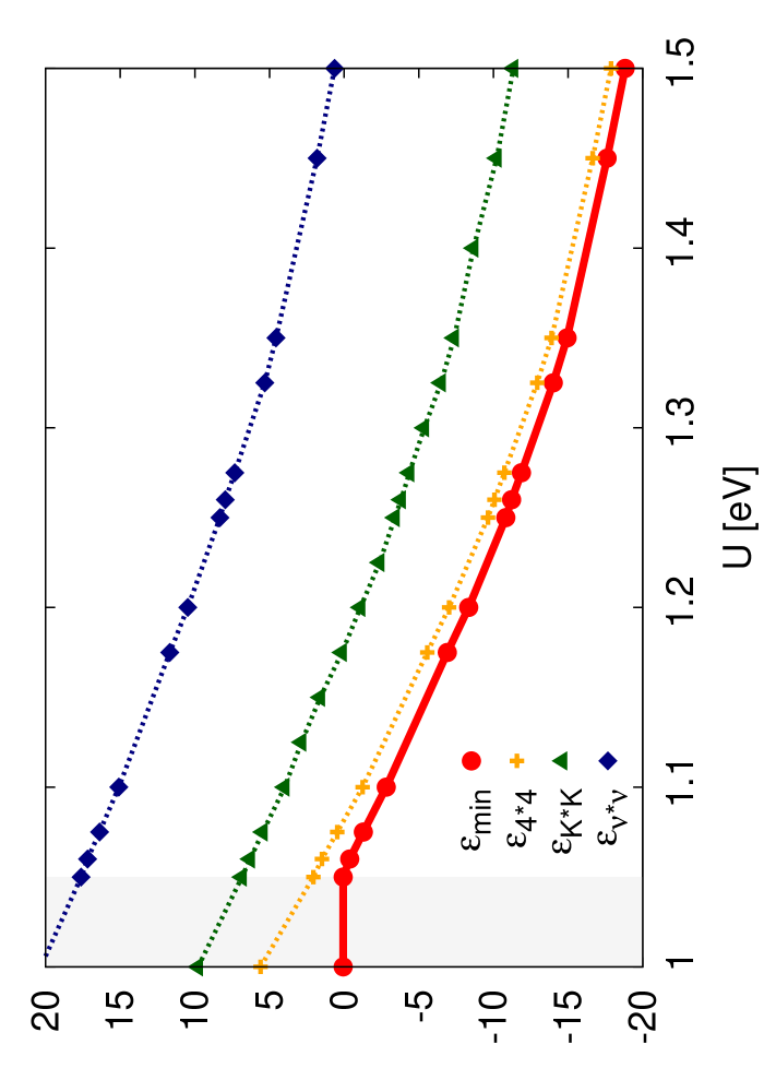
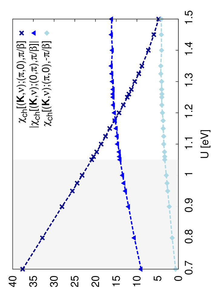
Figure 10: Lowest eigenvalue $\varepsilon_{\rm min}$ of $\chi_{d}$ compared with the approximations $\varepsilon_{4\times 4}$, $\varepsilon_{{\bf K}\times{\bf K}}$ and $\varepsilon_{\nu_{n}\times\nu_{n}}$. Matrix elements of $\chi_{ch}$ for ${\bf Q}=(\pi,\pi)$ and $\omega=0$ as a function of U.The parameters are $N_{c}=4$, $t=-0.25$ eV eV and $\beta=10$ eV^-1.

The results of our analysis, for different values of $U$, are shown in Fig. 10. We see that the eigenvalue $\varepsilon_{4\times 4}$ provides a quite accurate approximation to the exact minimal eigenvalue $\varepsilon_{\rm min}$ of the full generalized charge susceptibility for values of $U$ ($U>1.05$) where $\varepsilon_{\rm min}<0$. This illustrates that the matrix elements discussed above are really the dominating ones. Furthermore, we find that the “Fermi-level”-momentum approximation $\varepsilon_{{\bf K}\times{\bf K}}$ is also reasonably accurate, while the low-frequency $\varepsilon_{\nu\times\nu}$ is less accurate.

Fig. 10 (right panel) shows the dependence on $U$ for some of these matrix elements. The diagonal element for ${\bf K}={\bf K}^{\prime}=(\pi,0)$ and $\nu=\nu^{\prime}=\pi/\beta$ rapidly decreases with $U$, while the absolute value of the off-diagonal element in ${\bf K}$ for ${\bf K}=(\pi,0)$, ${\bf K}^{\prime}=(0,\pi)$ and $\nu=\nu^{\prime}=\pi/\beta$ is large and slowly increases with $U$. This matrix element is, in particular, due to the unequal spin contribution. In Sec. V we show how – in the case of $N_{c}=4$ cluster – this evolution is linked to the progressive stabilization of a RVB-dominated ground-state. The off-diagonal element in frequency for ${\bf K}={\bf K}^{\prime}=(\pi,0)$, $\nu=\pi/\beta$ and $\nu^{\prime}=-\pi/\beta$, instead, remains rather small.

The minimal eigenvalue $\varepsilon_{{\bf K}\times{\bf K}}$ of the $2\times 2$ matrix in ${\bf K}$ is given by

$$\varepsilon_{{\bf K}\times{\bf K}} \!=\! \chi_{ch}[(\pi\!,\!0),{\pi\over\beta};(\pi\!,\!0),{\pi\over\beta}]\!-\!|\chi_{ch}[(\pi\!,\!0),{\pi\over\beta};(0\!,\!\pi),{\pi\over\beta}]|$$ (15)

$$\!=\! \chi_{ch}^{diag}-t_{\bf{K}}$$

Evidently, when the magnitude of the off-diagonal element ($t_{\bf{K}}$) becomes equal to the diagonal element ($\chi_{ch}^{diag}$), the lowest eigenvalue $\varepsilon_{{\bf K}\times{\bf K}}$ goes negative (see Fig. 11). The (opposite) sign of the matrix elements in the $2\times 2$ matrix are such that the two components of the corresponding eigenvector have the same sign.

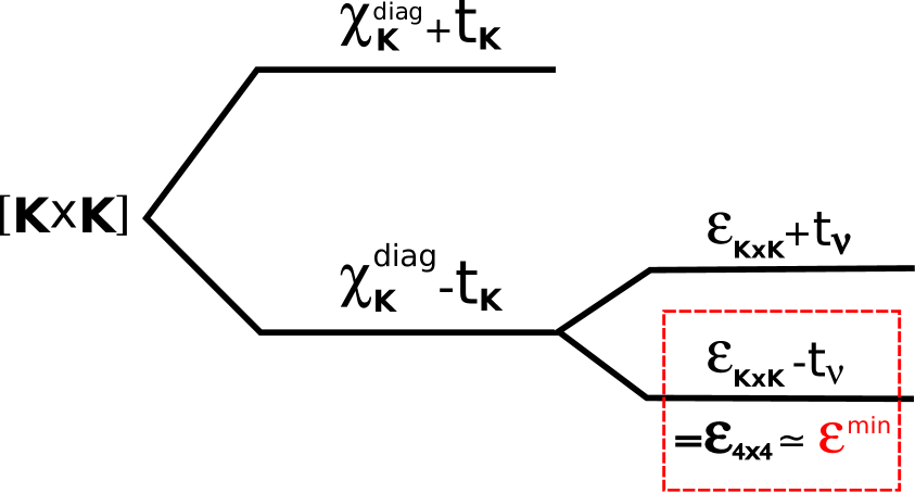
Figure 11: Schematic representation of the main diagonalization steps, determining the lowest ($1st$: dashed red box, and $2nd$) negative eigenvalues of $\chi_{ch}$, after the first/second level crossing has occurred.

By extending our analysis, we will then the considered the $4\times 4$ matrix. Its two lowest eigenvalues are shown in Fig. 12. The eigenvalue $\varepsilon_{{\bf K}\times{\bf K}}$ is further split into two by the small off-diagonal matrix elements for $\nu\neq\nu^{\prime}$ ($t_{\nu}$ in Fig.  11), in a bonding and anti-bonding state. Similarly to the $N_{c}=1$ case the components of the eigenvector corresponding to the lowest eigenvalue ($\varepsilon_{{\bf K}\times{\bf K}}-t_{\nu}$) have different signs for $\nu=-\pi/\beta$ and $\pi/\beta$. Then, the eigenvector corresponding to the second lowest eigenvalue, which vanishes at a larger $U\sim 1.35$, will have the two component $\nu=\pm\pi/\beta$ with the same sign.

Eventually, combining all the eigenvector signs, we obtain that the lowest eigenvalue is associated to an eigenvector with opposite sign components, while the second lowest is not. This evidently depends on the specific signs in Table 1. Hence, similar to the $N_{c}=1$ case, also for $N_{c}=4$, the singularities occurring in $\chi_{ch}$ will be actually responsible for the blowing up of the parquet decomposition (see Appendix A), with the significant exception of the first one encountered from weak-coupling.

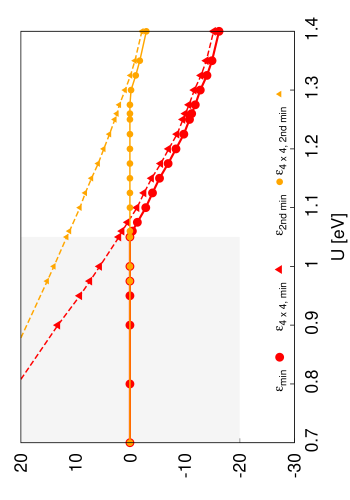
Figure 12: Calculated and approximate ($\varepsilon_{4\times 4}$) lowest two eigenvalues. The parameters are $N_{c}=4$, $t=-0.25$ eV and $\beta=10$ eV^-1.

If one considered also the generalized susceptibility in the particle-particle channel $\chi_{pp,\uparrow\downarrow}$, we would find an analogous trend. For the case considered here where $\chi_{pp}$ is real for ${\bf Q}=(0,0)$, it would show an eigenvalue going through zero slightly below $U=1.3$ eV. Similarly, the complex $\chi_{pp}$ for ${\bf Q}=(\pi,\pi)$ has a real eigenvalue going through zero slightly below $U=1.25$ eV. In such cases, the signs of the corresponding singular eigenvector components do not compensate, which yield to the strong low-frequency oscillations of the $\tilde{\Sigma}_{pp}$ data, presented in the previous section. Moreover, in the same parameter regime ($U\sim 1.3$), also the singularities of the lowest real eigenvalue of $\chi_{ch}$ for ${\bf Q}=(\pi,0)$ or for $(0,\pi)$ crossing zero do not cancel, leaving the spin channel as the only contribution of the parquet decomposition unaffected by singularities.

In summary, we find that the singularities in the generalized susceptibilities are actually reflected in a blowing up of the parquet decomposition in the corresponding channel(s). Due to the possible occurrence of compensating signs in the frequency components of the singular eigenvector of $\chi$, however, the correspondence is not complete. In fact, we find that the parquet decomposition remains well-behaved in all channels even beyond the value of $U$, where the first singularity appears in the Bethe-Salpeter equation for the charge channel (i.e., at $U\sim 1.05$ for $\beta=10$ eV^-1 in DCA with $N_{c}=4$), because of the compensating signs of the singular eigenvector. However, this is no longer the case for larger values of $U$, where the singular parts of $\chi_{ch}^{-1}$ and/ or $\chi_{pp}^{-1}$ add up in the parquet decomposition of the self-energy, making a separate (parquet) treatment of the corresponding scattering channels quite problematic. More specifically, in this regime, the absolute contribution from the totally irreducible diagrams to the self-energy at low-frequencies tends to be very large, and to a substantial extent, to be canceled by a very large particle-particle contribution. Beyond this compensations, it is also interesting to note that in Fig. 6 a sign-crossing is observed between the anomalous low frequency contributions of the irreducible and the $pp$ channel to the self-energy and their more conventionally behaved counter-parts at high-frequency. Hence, since the high-frequency behavior of the self-energy can be related to the lowest order perturbation theory, the sign crossings of the $pp$ and fully irreducible contribution at intermediate frequency represent an evident manifestation of the break-down of the perturbative description.

In order to go beyond this mostly formal interpretation of the singularities in the generalized susceptibilities (and of their effects on the parquet decomposition), in the next subsection we will improve our understanding of the underlying physics by a comparison with simplified model cases, where such singularities also appear.

V Physical interpretation of the singularities

V.1 Two level model

To improve our physical insight on the occurrence of the singularities, we start by considering one of the most basic case, where they appear, i.e., a simple two-level (impurity) model: This model has a Coulomb interaction $U$ on the ($N_{c}=1$) cluster site and no interaction on the bath site $b$ and an intersite hopping $V$. Specifically, we use $V=0.5$ eV, $\beta=5$ eV^-1 and we consider the half-filled case.

Fig. 13 shows the lowest eigenvalue $\varepsilon_{\rm min}$ of $\chi_{ch}$ for $\omega=0$ and the corresponding lowest eigenvalue $\varepsilon_{2\times 2}$ in Eq. (14) of the $2\times 2$ matrix containing matrix elements for $\nu=\pm\pi/\beta$. More specifically we also note that increasing $U$ increases the off-diagonal matrix element $\chi_{ch}(\pi/\beta;-\pi/\beta)$. Similarly as for the DMFT calculations of the previous section, when this element becomes equal to the diagonal element, $\varepsilon_{2\times 2}$ goes negative [Eq. (14)]. At this point, $\varepsilon_{2\times 2}$ becomes a rather good approximation to $\varepsilon_{\rm min}$, as it was also the case in Fig. 14. Hence, in this parameter range, we can limit our analysis to the lowest frequency sector ($\nu=\pm\pi/\beta$).

From the above discussion, we notice that the overall properties of the singularity of $\chi_{ch}$ in the two-level model appear qualitatively similar to the one of the DMFT calculations of the Hubbard model in Sec. IV.1. Differently from the latter case, however, in the two-level model, we have access to more intrinsic information, such as the exact ground state of the systems. This allows for a deeper investigation of the physical evolution associated with the singularities. In particular, we show how large the overlap of the ground state of the system with the singlet state

$${1\over\sqrt{2}}(|c\uparrow b\downarrow\rangle-|c\downarrow b\uparrow\rangle),$$ (16)

is, where two electrons, one on each site, form a valence bond: In the inset of Fig. 13, by increasing $U$, we clearly observe a monotonously enhanced weight of the singlet state of Eq. 16 in the ground state of the system.

In particular, the progressive change in the ground state is responsible of the (increasing/decreasing) trends of the (off-diagonal/diagonal) elements of $\chi_{ch}(\pm\pi/\beta;\pm\pi/\beta)$, driving, eventually, the sign-change of $\varepsilon_{\rm min}$.

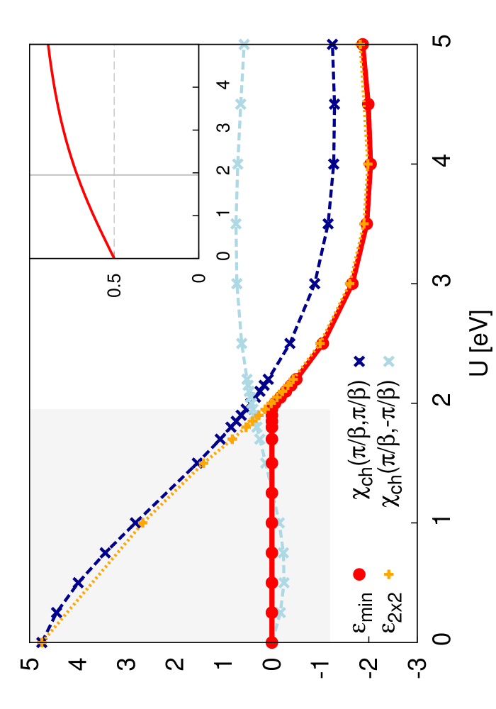
Figure 13: Diagonal and off-diagonal elements of $\chi_{ch}^{-1}$ for $\nu=\pm\pi/\beta$ of the two-level model as a function of $U$. The lowest eigenvalue is compared with the approximation in Eq. (14) for the eigenvalue. The weight of the singlet component in Eq. (16) is shown in the inset as a function of $U$. The parameters are $V=0.5$ eV and $\beta=5$ eV^-1.

Below we will continue by discussing the more significant $N_{c}=4$ case, and show in more detail how the formation of a negative eigenvalue of $\chi_{ch}$ is, in that case, associated with the formation of a resonance valence bond (RVB).

V.2 RVB state and pseudogap

In this subsection, we will show how the analysis of properties of the ground-state of the system can be extended to the case of $N_{c}=4$. Here, instead of the two-level model, we will exploit a preceding study of the pseudogap in the Hubbard model using a very different approach.pseudogap In fact, due to the relevance for the cuprate physics, the general problem of the pseudogap formation in the Hubbard model on a square lattice has been intensively investigated for embedded clusters, e.g., in DCA.otherpseudogapref ; Leo Based on studies for $N_{c}=4$ and $8$, it has recently been argued that, for a sufficiently large $U$, a localized state $|{\rm\psi}_{\rm loc}\rangle$ is formed on the cluster,pseudogap leading to pseudogap features. More specifically, by comparing correlation functions of the DCA calculation and for $|{\rm\psi}_{\rm loc}\rangle$, this state was identifiedpseudogap with a singlet, which –for $N_{c}=4$ we are considering here– takes the approximate form

$$|{\rm\psi}_{\rm loc}\rangle\!=\!{1\over\sqrt{2}}(c^{\dagger}_{(\pi,0)\uparrow}c^{\dagger}_{(\pi,0)\downarrow}-c^{\dagger}_{(0,\pi)\uparrow}c^{\dagger}_{(0,\pi)\downarrow})c^{\dagger}_{(0,0)\uparrow}c^{\dagger}_{(0,0)\downarrow}|{\rm vac}\rangle$$ (17)

Here, the ${\bf K}=(0,0)$ level is doubly occupied, while the levels ${\bf K}=(\pi,0)$ and $(0,\pi)$ are each doubly occupied with a probability of $\frac{1}{2}$. We now want to show that this state is closely related to the resonance valence bond (RVB) state.Liang88 Since the RVB state has no double-occupancy ($U\rightarrow\infty$), we can make this connection explicit in two steps. First we compare with a calculation for an isolated cluster with $t=-0.25$eV and a finite, intermediate value of $U=1.25$ eV, relevant for the discussion here. Afterwards, we compare these calculations for the isolated cluster with $U=1.25$ eV and $U=\infty$. We find a very large overlap ($\sim 0.92$) between $|{\rm\psi}_{\rm loc}\rangle$ of Eq. (17) and the ground-state of the isolated $U=1.25$ eV cluster. Secondly, we find that the overlap of the ground-state for the isolated cluster with $U=1.25$ eV to the $U=\infty$ RVB state is also large ($\sim 0.85$), the difference arising mainly from the double-occupancies. In fact, all configurations in real space with nonzero weight for the RVB state have similar weights also in the calculation for $U=1.25$ eV. In summary, $|{\rm\psi}_{\rm loc}\rangle$ in Eq. (17) is closely related to the ground-state of the isolated cluster at finite $U$, and, hence, apart from some residual double occupancy, to the RVB state.

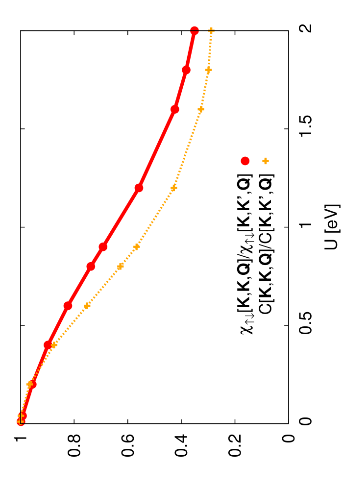
Figure 14: Ratio of $\chi_{\uparrow\downarrow}^{\bf K,K,Q}/\chi_{\uparrow\downarrow}^{{\bf K},{\bf K^{\prime}},{\bf Q}}$ for ${\bf K}=(0,\pi)$ and ${\bf K}^{\prime}=(\pi,0)$ and ${\bf Q}=(\pi,\pi)$. The figure also shows the ratio $C[{\bf K},{\bf K},{\bf Q}]/C[{\bf K},{\bf K}^{\prime},{\bf Q}]$ (Eq. 18). Matsubara labels have been suppressed; all Matsubara frequencies have their $n=0$ values. The parameters are $t=-0.25$ eV, $\beta=10$ eV^-1 and $N_{c}=4$.

We now want to show that the state in Eq. (17) is indeed formed and to relate this to the divergence of $\chi_{ch}$. We focus on the case $N_{c}=4$. As discussed in the context of Fig. 12, an important reason for the divergence is the behavior of $\chi_{ch}$ and in particular of $\chi_{\uparrow\downarrow}(k,k^{\prime},q)$ for ${\bf Q}=(\pi,\pi)$ and ${\bf K}$ and ${\bf K}^{\prime}$ equal to $(\pi,0)$ or $(0,\pi)$ at the lowest Matsubara frequencies. As $U$ is increased the element for ${\bf K}={\bf K}^{\prime}$ is reduced while the element for ${\bf K}\neq{\bf K}^{\prime}$ becomes large and negative. To make the connection between the formation of an RVB state and the divergence, we introduce

$$C({\bf K},{\bf K}^{\prime},{\bf Q})=\sum_{\nu\nu^{\prime}\omega}\chi_{\uparrow\downarrow}({\bf K},\nu;{\bf K}^{\prime},\nu^{\prime};{\bf Q},\omega).$$ (18)

Fig. 14 shows that the ratio between $C$ for ${\bf K}^{\prime}={\bf K}$ and ${\bf K^{\prime}}\neq{\bf K}$ behaves in a very similar way as the corresponding ratio for $\chi_{\uparrow\downarrow}({\bf K},\pi/\beta;{\bf K}^{\prime},\pi/\beta;{\bf Q},0)$ at the lowest Matsubara frequencies. The difference between the two curves is that $C$ contains a sum over all Matsubara frequencies. It is then not surprising that the two curves are similar. The quantity in Eq. (18) is easier to analyze. We use that $(1/\beta)\sum_{\nu}e^{i\tau\nu}=\delta(\tau)$, where the summation is over fermion or boson frequencies. Then

$${1\over\beta^{3}}C({\bf K},{\bf K}^{\prime},{\bf Q})=\langle c^{\dagger}_{{\bf K}\uparrow}c^{\phantom{\dagger}}_{{\bf K}+{\bf Q}\uparrow}c^{\dagger}_{{\bf K}^{\prime}+{\bf Q}\downarrow}c^{\phantom{\dagger}}_{{\bf K}^{\prime}\downarrow}\rangle$$ (19)

It is then easy to check that for the ground-state (17) the matrix element for ${\bf Q}=(\pi,\pi)$, ${\bf K}={\bf K}^{\prime}=(\pi,0)$ is zero, while it is $-\frac{1}{2}$ for ${\bf K}^{\prime}=(0,\pi)$. This would lead to a vanishing ratio in Fig. 14, in qualitative agreement with the actual calculation.

The second lowest state on the cluster is a triplet of the form

$${1\over\sqrt{2}}(c^{\dagger}_{(\pi,0)\uparrow}c^{\dagger}_{(0,\pi)\downarrow}+c^{\dagger}_{(0,\pi)\uparrow}c^{\dagger}_{(\pi,0)\downarrow})c^{\dagger}_{(0,0)\uparrow}c^{\dagger}_{(0,0)\downarrow}|{\rm vac}\rangle.$$ (20)

It should be emphasized here, that if this had been the lowest state, we would have got exactly the opposite result to above, i.e., a large matrix element for ${\bf K}={\bf K}^{\prime}$ and a small matrix element for ${\bf K}^{\prime}=(0,\pi)$.

Our analysis of the $N_{c}=4$ DCA results demonstrate thus that in the regime, where a pseudogap is observedpseudogap for sufficiently large $U$, i) the essential physics can be traced back to a state of RVB character, and ii) that the hallmark of such RVB character is directly reflected in large off-diagonal elements of $\chi$ in the Fermi-momentum subspace [$(0,\pi)$, $(\pi,0)$] . The latter result is quite important for discussing the interpretation of the observed singularities in the parquet decomposition of the DCA results. At large enough $U$, in fact, an underlying RVB state has also been related to the formation of a pseudogap.pseudogap Thus, in this regime, the trends towards a RVB ground-state would be the common underlying reason behind onset a pseudogap and the formation of negative eigenvalues of $\chi_{ch}$ and the associated strong frequency oscillations of the parquet decomposition.

We note, finally, that the considerations discussed here are rigorously valid for the parquet singularities of the $N_{c}=4$ data. They will remain largely applicable to the cases of small DCA clusters discussed in the present work. Modifications might be possible, instead, in the cases of extended clusters, where a pseudogap spectral weight suppression can be induced also at much weaker-coupling by long-ranged (spin) correlationsSchaefer2015A . For such larger DCA clusters, the parquet decompositions is still numerically challenging.

V.3 Charge susceptibility and closeness to Mott transition

Some further physical insight into this problem can be gained starting from the general observation that, when $U$ is increased, the charge susceptibility is suppressed, while the spin susceptibility becomes large. It is then not surprising that we find rather different behavior of $\chi_{ch}$ and $\chi_{sp}$. The charge susceptibility can be expressed in terms of the generalized charge susceptibility

$$\chi_{ch}(q)={1\over N_{c}\beta^{2}}\sum_{kk^{\prime}}\chi_{ch}(k;k^{\prime};q).$$ (21)

We now use Eq. (24) to rewrite the susceptibility as

$$\chi_{ch}=\sum_{i}\sum_{kk^{\prime}}\langle k|i\rangle\varepsilon_{i}\langle i|k^{\prime}\rangle=\sum_{i}\varepsilon_{i}|\sum_{k}\langle k|i\rangle|^{2},$$ (22)

where $\varepsilon_{i}$ and $|i\rangle$ are the eigenvalues and eigenvectors, respectively, of $\chi_{ch}$. The $q$ dependence is not shown explicitly. We find

$$\sum_{i}|\sum_{k}\langle k|i\rangle|^{2}=\sum_{kk^{\prime}}\sum_{i}\langle k|i\rangle\langle i|k^{\prime}\rangle=N_{k},$$ (23)

where $N_{k}$ is the number of $k$ values and thereby the number of eigenvalues. Thus, except “pathological” cases of strongly varying overlaps $\langle k|i\rangle$ occurnote_evsdem , $|\sum_{k}\langle k|i\rangle|^{2}$ will be in general not small. This, together with $\chi_{d}$ being small, puts then constraints on the eigenvalues.

For $N_{c}=1$ it has been shown that all eigenvalues of $\chi_{ch}(k,k^{\prime},q=0)$ are positive for small $U$.divergence For large $U$, a small $\chi_{ch}(q=0)$ can be obtained if all eigenvalues are small (and possibly all positive) or if some eigenvalues are negative. Since individual matrix elements are large, the former could not be the case. Then the strong suppression of $\chi_{ch}(q=0)$ for large $U$ is expected to require that some eigenvalues are negative, although pathological cases may be found where this is not the case. Similar arguments apply for larger clusters for values of $q$ where the eigenvalues are real and positive for small $U$. The appearance of negative eigenvalues as $U$ is increased and, hence, of the huge low-frequency oscillations in the the parquet decomposition, should be a consequence of a gradual suppression of charge fluctuation as the system approaches a Mott transition. This supports an earlier preliminary interpretation (within DMFT) of a negative eigenvalue as a precursor effect of the Mott transition.divergence The DCA results, suggesting an intrinsic connection with the RVB physics and the pseudogap formation, implies a more profound, and highly non-perturbative, picture of the electronic correlations in two-dimensional lattice systems.

VI Conclusions

We have calculated the two-particle vertex function in DMFT and DCA for the Hubbard model. The vertex function was then exploited to perform a parquet decomposition of the DCA self-energy. The purpose of such decomposition was similar as for the recently introduced fluctuation diagnostic approach,FluctDiag i.e., to improve our understanding of the physical origin of the numerical results for the self-energy. In comparison to the latter approach, the parquet decomposition allows -in principle- for a more direct formulation, which does not require any representation change in the equation of motion for the self-energy. However, as we discussed in this work, as opposed to the fluctuation diagnostics procedure, its usage poses also important new challenges.

While the parquet decomposition works relatively smoothly in the perturbative regime and allows one to evaluate quantitatively the role played by the different channels, for larger values of $U$ and moderate doping, some of its terms start to display very large oscillations at small frequencies. This renders it impossible to disentangle the role of the channels affected by such oscillations. We should note, however, that in all cases considered we could always find, even at strong coupling, at least one well-behaved term in the parquet decomposition (which was the spin contribution, $\tilde{\Sigma}_{sp}$, for the $2d$ and $3d$ Hubbard model close to/at half-filling). This has been interpreted as a specific indication emerging from the parquet decomposition of a predominance of that well-behave channel. In this way the predictions of the parquet decomposition of $\Sigma$ provide a qualitatively similar outcomeFluctDiag to those of the fluctuation diagnostics. Unlike the former, the latter approach, appears not to be affected at all by entering in non-perturbative regime.

Beyond the physical insight in the self-energy, our results are also relevant for the future developments of forefront methods in quantum many body physics. In fact, several recently proposed computational schemes have been based on the parquet decomposition, introducing approximations for the totally irreducible diagrams, and then calculating the reducible diagrams via the parquet equations.PA_Jarrell ; DGA ; Multiscale ; DFparquet The results above, however, show that the contribution from the irreducible diagrams becomes highly complicated for strongly correlated systems, even diverging for certain values of $U$. This suggests that all schemes based on the parquet decomposition above might encounter unforeseen problems in the intermediate-to-strong correlated regime. However, we should recall that the generalized susceptibilities in Matsubara space are not directly measurable quantities. Hence, one may wonder, whether alternatives to the conventional parquet decomposition for classifying the Feynman diagrams could be found, in order to improve the description of electronic correlations in the intermediate coupling regimes and avoid the singularities.

In the specific context of our DMFT and DCA analysis, we have demonstrated that the singularities of some terms of the parquet decomposition of the self-energy is directly related to the divergencies of $\chi_{ch}^{-1}$ and $\chi_{pp}^{-1}$ at intermediate $U$ values. In particular, we showed that the divergence of $\chi_{ch}^{-1}$ is related to the suppression of charge fluctuations. This represents an early, non-perturbative, manifestation of the Mott-Hubbard physics. The relation of such singularities to a RVB state and to the formation of a pseudogap has also been investigated for the case of the $N_{c}=4$ DCA clusters, making progress towards a theoretical understanding of the highly non-trivial physics of strong electron correlations in two-dimensions.

VII ACKNOWLEDGMENTS

We thank E. Gull and P. Thunström for insightful discussions. We acknowledge financial support from the Austrian Science Fund (FWF) through the Doctoral School Solid for Fun (W1243, T.S.) the project I610-N16 (T.S,G.R.), and the SFB-ViCoM F41 (A.T.). J.M. acknowledges financial support from MINECO (MAT2012-37263-C02-01). G.S. acknowledges financial support from research unit FOR 1346 of the Deutsche Forschungsgemeinschaft. We also thank K. Kölbl for graphical advices.

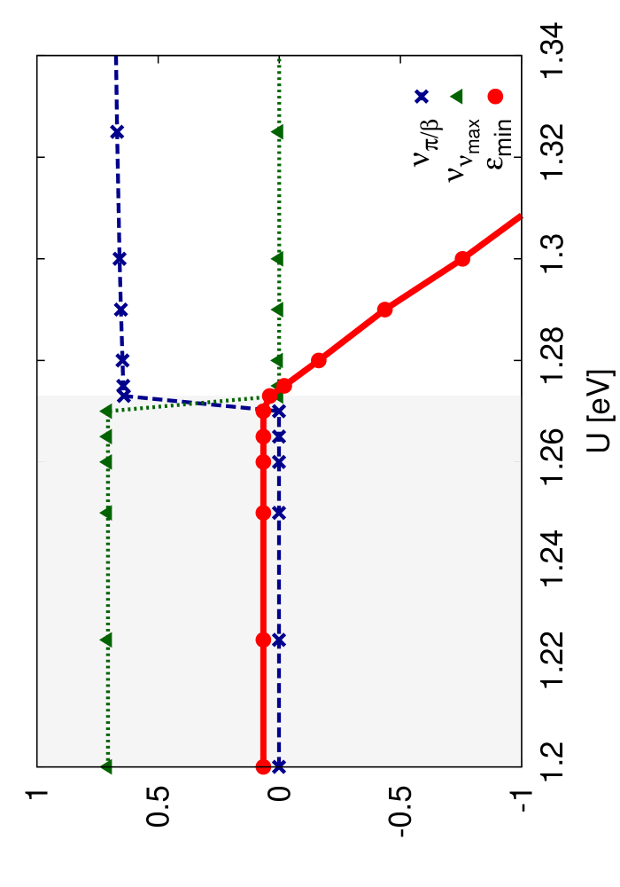
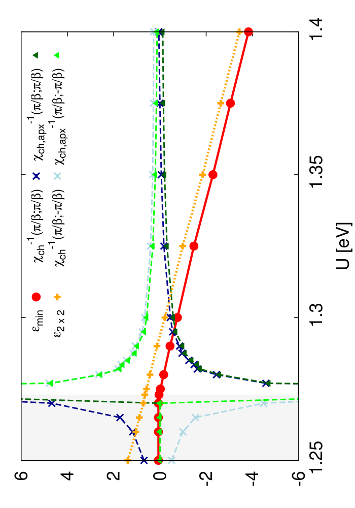
Figure 15: DMFT results illustrating the change of sign of the eigenvalues of $\chi_{\text{ch}}$ for the parameters $t=-0.25$ eV, $\beta=10$ eV^-1, $n=1$ and $N_{c}=1$. Left panel: The lowest eigenvalue of $\chi_{\text{ch}}(\nu,\nu^{\prime}\omega=0)$ and the elements of the corresponding eigenvector for $\nu=\pm\pi/\beta$ and $\nu=\pm\nu_{\text{max}}$ are compared (see also text below Eq. (13)). Right panel: Diagonal and off-diagonal elements of $\chi^{-1}_{\text{ch}}$ for $\nu=\pm\pi/\beta$. $\chi_{\text{ch,apx}}^{-1}$ is an approximation to $\chi_{\text{ch}}^{-1}$, using only the lowest eigenvalue in Eq. (24).

Appendix A Formation of negative eigenstate at $\omega=0$

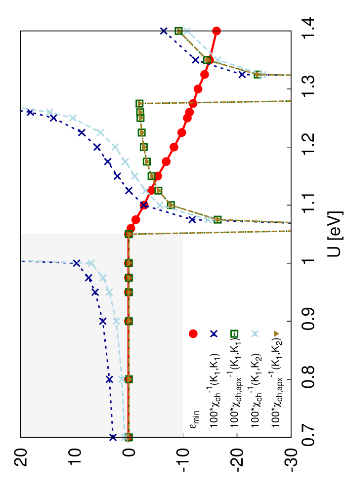
Figure 16: Calculated ($\chi_{\text{ch}}^{-1}$) and approximated ($\chi_{\text{ch,apx}}^{-1}$) matrix elements in DCA for the parameters $N_{c}=4$, $t=-0.25$ eV, $n=1$ and $\beta=10$ eV^-1. Shown are the two momentum points $K_{1}=(0,\pi)$ and $K_{2}=(\pi,0)$.

In this Appendix we further elaborate on the divergence of $\chi_{\text{ch}}^{-1}$ at $\omega=0$ in Sec. IV and the corresponding evolution of the singular eigenvalue of $\chi_{\text{ch}}$. Specifically, in order to analyze the role played by the lowest eigenvalue of the generalized susceptibility, we express the inverse of $\chi_{\text{ch}}$ in the basis of the eigenvalues ($\varepsilon_{i}$) and the eigenvectors ($|i\rangle$) of $\chi_{\text{ch}}$:

$$\chi_{\text{ch}}^{-1}=\sum_{i}|i\rangle\varepsilon_{i}^{-1}\langle i|.$$ (24)

An approximate expression, $\chi_{\text{ch,apx}}^{-1}$, can then be obtained by restricting the sum to the lowest eigenvalue of $\chi_{\text{ch}}$.

We now illustrate the usefulness of the representation Eq. 24 by applying it first to the case of DMFT ($N_{c}=1$). In Fig. 15, the evolution of the exact and approximate eigenvalues with interaction strength $U$ is shown for $t=-0.25$ eV, $n=1$ and $\beta=10$ eV^-1. For $U<1.275$, where the lowest eigenvalue is positive, the contribution for $\nu=\pm\pi/\beta$ is approximately zero, because the corresponding (weak-coupling) eigenvector has almost no weight for these frequencies. $\chi_{\text{ch}}^{-1}$ becomes large already for $U$ slightly smaller than $1.275$, where the approximate eigenvalue is small but positive. Here, a low-lying “resonance” gives a large contribution. When the resonance goes through zero and becomes a “bound state” (negative eigenvalue) for the matrix of the generalized susceptibility, the sign of $\chi_{\text{ch}}^{-1}$ (and hence also that of $\Gamma_{\text{ch}}$) changes. For $U\geq 1.275$, $\chi_{\text{ch,apx}}^{-1}$ provides a quite good approximation of $\chi_{\text{ch}}^{-1}$, showing that the large values of $\chi_{\text{ch}}^{-1}$ are mainly due to this “bound-state”. As $U$ is increased further, the lowest eigenvalue gets more negative, and the matrix elements of $\chi_{\text{ch}}^{-1}$ are reduced. The basic character of $\chi_{\text{ch}}$, however, remains qualitatively different compared with smaller values of $U$.

This analysis can also be extended to the case of DCA. Fig. 16 shows matrix elements of the DCA $\chi_{\text{ch}}^{-1}$ (at half-filling and $\beta=10.0$) compared with the approximation $\chi_{\text{ch,apx}}^{-1}$ where only negative eigenvalues are considered in the inversion in Eq. (24). For $U<1.05$ all eigenvalues are are positive and $\chi_{\text{ch,apx}}^{-1}$ is zero. However, there is a resonance for $U$ close to 1.05, as is also indicated by the small value of $\varepsilon_{4\times 4}$ (see Sec. IV for the corresponding definitions). This leads to a large contribution to $\chi_{\text{ch}}^{-1}$ for $U$ close to 1.05. As the lowest eigenvalue goes negative at $U=1.05$, the signs of some large matrix elements of $\chi_{\text{ch}}^{-1}$ change [see Eq. (24)]. At the same time $\chi_{\text{ch,apx}}^{-1}$ becomes a rather good approximation to $\chi_{\text{ch}}^{-1}$. Increasing $U$ further, a second resonance forms, as is also seen by the small value of the second lowest eigenvalue in the $4\times 4$ space. This leads to very large values of $\chi_{\text{ch}}^{-1}$ for $U>1.2$, which are missed by $\chi_{\text{ch,apx}}^{-1}$. For $U>1.35$ this resonance is converted to a negative eigenvalue, signs of matrix elements of $\chi_{\text{ch}}^{-1}$ change, and $\chi_{\text{ch,apx}}^{-1}$ again becomes a good approximation of $\chi_{\text{ch}}^{-1}$.

Appendix B General structure of the $2\times 2$ singular matrix

The following generic matrix is related to the discussion in the main text:

$$M=\begin{pmatrix}a&b\\ b&a\end{pmatrix},$$ (25)

where $a,b\in\mathds{R}$ and $b>0$.

The eigenvalues and eigenvectors are given by $\lambda_{\mp}=a\mp b$ and $\mathbf{v}_{\mp}=(\mp 1,1)/\sqrt{2}$.

Hence, the spectral representation of the inverse of $M$ reads:

$$M^{-1}=\frac{1}{2(a-b)}\begin{pmatrix}1&-1\\ -1&1\end{pmatrix}+\frac{1}{2(a+b)}\begin{pmatrix}1&1\\ 1&1\end{pmatrix}$$ (26)

When the first eigenvalue vanishes ($a=b$) the first term of the matrix $M^{-1}$ diverges, while the sum over all its matrix elements stays finite, because the sum over the matrix elements in the first term exactly vanishes due to the antisymmetry of the corresponding eigenvector. Hence, the sum over all matrix elements, originating from the second term in Eq. (26), yields the finite result $1/a$. For $a=-b$, however, one encounters the divergence of the second eigenvalue. In this case also the sum over all matrix elements diverges, as the (equal) signs of the corresponding eigenvector no longer cancel it.

References

- (1) L. Hedin and S. Lundqvist, Solid State Physics 23, 1 (1969).
- (2) A. A. Abrikosov, L. P. Gorkov (Autor), F. A. Davis, Methods of Quantum Field Theory in Statistical Physics (Dover, New York, 1963).
- (3) L. Hedin, Phys. Rev. 139, A796 (1965).
- (4) F. Aryasetiawan, O. Gunnarsson, Rep. Prog. Phys. 61, 237 (1998).
- (5) W. G. Aulbur, L. Jonsson, and J. W. Wilkins, Solid State Physics 54, 1 (2000).
- (6) F. Aryasetiawan, O. Gunnarsson, Phys. Rev. Lett. 74, 3221 (1995).
- (7) P. Minnhagen, J. Phys. C 7, 3013 (1974); 8, 1535 (1975).
- (8) N.E.Bickers and D.J.Scalapino, Phys. Rev. Lett. 62, 961 (1989).
- (9) W. Metzner, M. Salmhofer, C. Honerkamp, V. Meden, and K. Schönhammer Rev. Mod. Phys. 84, 299 (2012).
- (10) For a review, see, e.g., N. E. Bickers, Int. J. Mod. Phys. B 5, 253 (1991) and in Theoretical Methods for Strongly Correlated Electrons, edited by D. Senechal, A. Tremblay, and C. Bourbonnais (Springer-Verlag, New York, 2004), chapter 6.
- (11) V. Janiŝ, J. Phys.: Condens. Matter 10, 2915 (1998); Phys. Rev. B 60, 11345 (1999).
- (12) S. X. Yang, H. Fotso, J. Liu, T. A. Maier, K. Tomko, E. F. D’Azevedo, R. T. Scalettar, T. Pruschke, and M. Jarrell, Phys. Rev. E 80, 046706 (2009); Ka-Ming Tam, H. Fotso, S.-X. Yang, Tae-Woo Lee, J. Moreno, J. Ramanujam, and M. Jarrell, Phys. Rev. E 87, 013311 (2013).
- (13) W. Metzner and D. Vollhardt, Phys. Rev. Lett. 62, 324 (1989); M. Jarrell, Phys. Rev. Lett. 69, 168 (1992); A. Georges, G. Kotliar, W. Krauth, and M. Rozenberg, Rev. Mod. Phys. 68, 13 (1996).
- (14) T. Maier, M. Jarrell, T. Pruschke, and M. H. Hettler, Rev. Mod. Phys. 77, 1027 (2005);
- (15) M. H. Hettler, A. N. Tahvildar-Zadeh, M. Jarrell, T. Pruschke, and H. R. Krishnamurthy, Phys. Rev. B 58, R7475 (1998); M. H. Hettler, M. Mukherjee, M. Jarrell,and H. R. Krishnamurthy, Phys. Rev. B 61, 12739 (2000).
- (16) G. Kotliar, S. Y. Savrasov, G. Palsson, and G. Biroli Phys. Rev. Lett. 87, 186401 (2001).
- (17) J. E. Hirsch and R. M. Fye, Phys. Rev. Lett. 56, 2521 (1986).
- (18) E. Gull, A. J. Millis, A. I. Lichtenstein, A. N. Rubtsov, M. Troyer, and P. Werner, Rev. Mod. Phys. 83, 349 (2011).
- (19) For a systematic and extensive comparison of extrapolated DCA data w.r.t. other techniques, see: J. P. F. LeBlanc, A. E. Antipov, F. Becca, I. W. Bulik, Garnet Kin-Lic Chan, Chia-Min Chung, Youjin Deng, M. Ferrero, T. M. Henderson, C. A. Jiménez-Hoyos, E. Kozik, Xuan-Wen Liu, A. J. Millis, N. V. Prokof’ev, M. Qin, G. E. Scuseria, Hao Shi, B. V. Svistunov, L. F. Tocchio, I. S. Tupitsyn, S. R. White, Shiwei Zhang, Bo-Xiao Zheng, Zhenyue Zhu, E. Gull, Phys. Rev. X 5, 041041 (2015).
- (20) A. Macridin, B. Moritz, M. Jarrell, and Th. Maier, Phys. Rev. Lett. 97, 056402 (2006).
- (21) O. Gunnarsson, G. Sangiovanni, A. Valli, and M. W. Haverkort, Phys. Rev. B 82, 233104 (2011).
- (22) Jan Kuneŝ, Phys. Rev. B 83, 085102 (2011).
- (23) G. Rohringer, A. Valli, and A. Toschi, Phys. Rev. B 86, 125114 (2012).
- (24) H. Park, K. Haule, and G. Kotliar, Phys. Rev. Lett. 107, 137007 (2011).
- (25) H. Hafermann, Phys. Rev. B 89 , 235128 (2014).
- (26) Gang Li, N. Wentzell, P. Pudleiner, P. Thunström, and K. Held, arXiv:1510.03330.
- (27) A. Toschi, A. A. Katanin, and K. Held, Phys. Rev. B 75, 045118 (2007); K. Held, A. A. Katanin, and A. Toschi, Prog. Theor. Phys. Suppl. 176, 117 (2008).
- (28) A. N. Rubtsov, M. I. Katsnelson, and A. I. Lichtenstein, Phys. Rev. B 77, 033101 (2008); H. Hafermann, G. Li, A. N. Rubtsov, M. I. Katsnelson, A. I. Lichtenstein, and H. Monien, Phys. Rev. Lett. 102, 206401 (2009).
- (29) G. Rohringer, A. Toschi, H. Hafermann, K. Held, V. I. Anisimov, and A. A. Katanin, Phys. Rev. B 88, 115112 (2013).
- (30) C. Taranto, S. Andergassen, J. Bauer, K. Held, A. Katanin, W. Metzner, G. Rohringer, and A. Toschi, Phys. Rev. Lett. 112, 196402 (2014); N. Wentzell, C. Taranto, A. Katanin, A. Toschi, and S. Andergassen Phys. Rev. B 91 045120 (2015).
- (31) T. Ayral and O. Parcollet, Phys. Rev. B 92, 115109 (2015).
- (32) M. Kitatani, N. Tsuji, and H. Aoki Phys. Rev. B 92, 085104 (2015).
- (33) C. Slezak, M. Jarrell, Th. Maier, and J. Deisz, J. Phys.: Condens. Matter 21 435604 (2009).
- (34) S.-X. Yang, H. Fotso, H. Hafermann, K.-M. Tam, J. Moreno, T. Pruschke, and M. Jarrell, Phys. Rev. B 84, 155106 (2011).
- (35) G. Rohringer, A. Toschi, A. Katanin, and K. Held, Phys. Rev. Lett. 107, 256402 (2011).
- (36) A. E. Antipov, E. Gull, and S. Kirchner, Phys. Rev. Lett. 112, 226401 (2014).
- (37) J. Otsuki, H. Hafermann, and A. I. Lichtenstein, Phys. Rev. B 90, 235132 (2014).
- (38) T. Schäfer, F. Geles, D. Rost, G. Rohringer, E. Arrigoni, K. Held, N. Blümer, M. Aichhorn and A. Toschi, Physical Review B 91, 125109 (2015).
- (39) T. Schäfer, A. Toschi, and J.M. Tomczak, Physical Review B 91, 121107 (2015).
- (40) P. Pudleiner, T. Schäfer, D. Rost, G. Li, K. Held, and N. Blümer, arXiv:1602.03748 (2016).
- (41) D. Hirschmeier, H. Hafermann, E. Gull, A. I. Lichtenstein, A. E. Antipov, Phys. Rev. B 92, 144409 (2015).
- (42) O. Gunnarsson, T. Schäfer, J.P.F. LeBlanc, E. Gull, J. Merino, G. Sangiovanni, G. Rohringer, and A. Toschi, Phys. Rev. Lett. 114, 236402 (2015).
- (43) N. F. Berk and J. R. Schrieffer, Phys. Rev. Lett. 17, 433 (1966).
- (44) D. J. Scalapino, Rev. Mod. Phys. 84, 1383 (2012).
- (45) B. Kyung, S. S. Kancharla, D. Senechal, A.-M.S. Tremblay, M. Civelli, and G. Kotliar, Phys. Rev. B 73, 165114 (2006). A. Macridin, M. Jarrell, T. Maier, P.R.C. Kent, and E. D’Azevedo, Phys. Rev. Lett. 97, 036401 (2006).
- (46) N. Bulut, D. J. Scalapino, and S. R. White, Phys. Rev. B 47, 2742 (1993).
- (47) K. Haule, A. Rosch, J. Kroha, and P. Wölfle, Phys. Rev. Lett. 89, 236402 (2002).
- (48) T. Schäfer, G. Rohringer, O. Gunnarsson, S. Ciuchi, G. Sangiovanni, and A. Toschi, Phys. Rev. Lett. 110, 246405 (2013).
- (49) V. Janiš and V. Pokorny, Phys. Rev. B 90, 045143 (2014).
- (50) S.-X. Yang, H. Fotso, H. Hafermann, K.-M. Tam, J. Moreno, T. Pruschke and M. Jarrell, arXiv:1104.3854v1 (unpublished appendix).
- (51) E. Kozik, M. Ferrero, and A. Georges, Phys. Rev. Lett. 114, 156402 (2015).
- (52) A. Stan, P. Romaniello, S. Rigamonti, L Reining and J.A. Berger New J. of Physics 17 093045 (2015).
- (53) R. Rossi and F. Werner, J. Phys. A 48, 485202 (2015).
- (54) T. Ribic, G. Rohringer, and K. Held, arXiv:arXiv:1602.07161.
- (55) P. W. Anderson, Science 235, 1196 (1987); S. Liang, B. Doucot, and P. W. Anderson, Phys. Rev. Lett. 61, 365 (1988).
- (56) E. Dagotto, Rev. Mod. Phys. 66, 763 (1994).
- (57) D. J. Scalapino, J. Superconductivity Novel Magnetism, 19, 195 (2006).
- (58) See, e.g., A. Toschi, M. Capone and C. Castellani, Phys. Rev. B 72, 235118 (2005); D. Nicoletti, O. Limaj, P. Calvani, G. Rohringer, A. Toschi, G. Sangiovanni, M. Capone, K. Held, S. Ono, Yoichi Ando, and S. Lupi Phys. Rev. Lett. 105, 077002 (2010).
- (59) G. Rohringer, New routes toward a theoretical treatment of nonlocal electronic correlations, PhD thesis, TU Vienna (2014).
- (60) S. Hummel, Asymptotic behavior of two-particle vertex functions in dynamical mean-field theory, Master thesis, TU Vienna (2014).
- (61) T. Schäfer, Electronic correlations at the two-particle level, Master thesis, TU Vienna (2013).
- (62) We note that, by reducing the weight of this eigenvector will become distributed over several low-lying frequencies, but the general picture, as well as the qualitative difference to the weak-coupling regime, remains similar in the whole temperature interval we considered.
- (63) For and is, in general, a complex matrix. A few eigenvalues, however are real, and one of these goes through zero, though for slightly larger coupling, i.e., between and eV. For is, in general, also a complex matrix. However, in this case already perturbation theory can give a negative real eigenvalue, and the study of is therefore not very interesting.
- (64) J. Merino and O. Gunnarsson, J. Phys.: Cond. Matter. 25, 052201 (2013); Phys. Rev. B 89, 245130 (2014); arXiv:1310.4597.
- (65) See, e.g., A. Macridin, M. Jarrell, Thomas Maier, P. R. C. Kent, and E. D’Azevedo, Phys. Rev. Lett. 97, 036401 (2006); A. Macridin, M. Jarrell, Phys. Rev. B 78, 241101(R) (2008); P. Werner, E. Gull, O. Parcollet, and A. J. Millis, Phys. Rev. B 80, 045120 (2010); G. Sangiovanni and O. Gunnarsson, Phys. Rev. B 84, 100505(R); E. Gull and A. J. Millis, Phys. Rev. B 86, 241106(R) (2012); J. P. F. LeBlanc and E. Gull, Phys. Rev. B 88, 155108 (2013).
- (66) See also related work for Anderson impurities in a host having, in particular, alkali-doped fullerene in mind: L. De Leo, M. Fabrizio, PRB 69, 245114 (2004); PRL 94, 236401 (2005).
- (67) It is worth stressing, that – in the light of the recent results obtained via the fluctuation diagnosticsFluctDiag - the occurrence of strongly varying matrix elements looks unlikely to be realized in secondary scattering channels, such as the charge channel in our case. Rather, the secondary nature of the (here: charge) channel would be reflected in a relatively featureless and smooth matrix element behavior of the (corresponding) generalized susceptibility.