LARGE-$N$ PION SCATTERING, FINITE-TEMPERATURE EFFECTS AND THE RELATIONSHIP OF THE $f_{0}(500)$ WITH CHIRAL SYMMETRY RESTORATION

Abstract

In this work, we review how the mass and the width of the $f_{0}(500)$ pole behave in a regime where temperature is below the critical chiral transition value. This is attained by considering a large-$N$ $O(N+1)/O(N)$ invariant Non-Linear Sigma Model (NLSM) such that we can study the dynamical generation of a $f_{0}(500)$ resonance. Introducing thermal effects via the imaginary time formalism allows us to study the behavior of the pole and relate it to chiral restoration.

12.39.Fe, 11.10.Wx, 11.15.Pg

1 Introduction

As lattice simulation results show [1, 2], analyzing low-energy phenomena as chiral symmetry restoration is needed for a proper description of the hadronic matter created in relativistic heavy ion collisions experiments (such as LHC-ALICE). Here we review a scenario [3] where a set of massless large-$N$ Nambu-Goldstone bosons [4] interact with themselves and dynamically generate a scalar resonance (the $f_{0}(500)$), thus breaking the chiral symmetry, which should be restored when considering a thermal bath below the critical value; after attaining this, and since the pions do not gain thermal masses, we obtain that the chiral restoration is a second-order phase transition.

2 Ellastic pion-pion scattering

2.1 Zero-temperature Regime

We begin by considering the following $O(N+1)/O(N)$ Nonlinear Sigma Model [4] with a metric and its associated vacuum constraint given by

$$\mathcal{L}_{NLSM}=\frac{1}{2}g_{ab}(\pi)\partial_{\mu}\pi^{a}\partial^{\mu}\pi^{b},$$ (1)

$$g_{ab}(\pi)=\delta_{ab}+\frac{1}{NF^{2}}\frac{\pi_{a}\pi_{b}}{1-\pi^{2}/NF^{2}}.$$ (2)

$$f_{\pi}^{\,2}=NF^{2}.$$ (3)

After expanding the non-diagonal term in (2) and reminding that we only want to study elastic scattering processes, we obtain the Feynman diagram and rule given in the left side of Fig 1, whose loop integral in the Dimensional Regularization scheme reads [5]:

$$J(s)=J_{\epsilon}(\mu)+\frac{1}{16\pi^{2}}\ln\left(\frac{\mu^{2}}{-s}\right),$$ (4)

$$J_{\epsilon}(\mu)=\frac{1}{16\pi^{2}}\left[\frac{2}{\epsilon}+\ln 4\pi-\gamma-\ln\mu^{2}\right]+\mathcal{O}(\epsilon).$$ (5)

Its proper renormalization is attained by redefining the 4-pion vertex as [6]

$$\frac{s}{NF^{2}}\rightarrow\frac{s}{NF^{2}}G_{0}(s),\,G_{0}(s)=1+\sum_{k=1}^{\infty}{g_{0,\,k}\left(\frac{s}{F^{2}}\right)^{k}}.$$ (6)

After considering this, we will absorb the divergence (5) in the bare function $G_{0}(s)$ as $G_{R}^{\,-1}(s,\mu)=G_{0}^{\,-1}(s)-sJ_{\epsilon}(s)/F^{2}$, where $G_{R}(s,\mu)$ is written as a series expansion of a set of renormalized low energy constants $g_{R,\,k}(\mu)$. Then, the amplitude reads

$$A_{R}(s)=\frac{s}{NF^{2}}\frac{G_{R}(s;\mu)}{1-\frac{s\,G_{R}(s;\mu)}{32\pi^{2}F^{2}}\ln\left(\frac{\mu^{2}}{-s}\right)}.$$ (7)

The partial wave associated to the scalar channel $I=J=0$ in the large-$N$ limit is given by

$$a_{00}(s)=\frac{1}{64\pi}\int_{-1}^{1}{NA_{R}(s)P_{0}(\cos\theta)d(\cos\theta)}.$$ (8)

This can be fitted to a proper set of data (both experimental and phenomenological) after choosing a scale compatible with $g_{R,\,k}(\mu)=0$. The results are shown in Fig. 2, and the parameters are listed in Table 1. We do not take into account data neither close to the first threshold (where the pion mass matters) nor above 800 MeV (since strangeness is not considered).

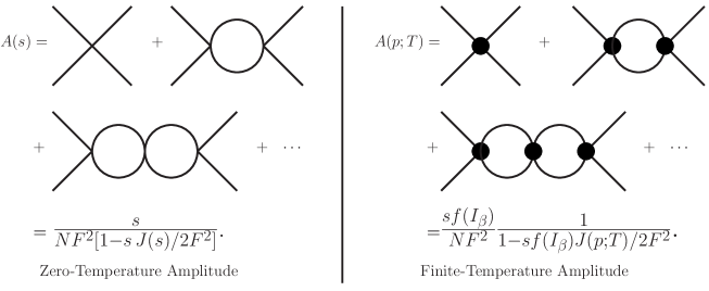
Figure 1: Zero-Temperature and Finite-Temperature scattering amplitude for massless pions. The black circle represents the effective thermal vertex.

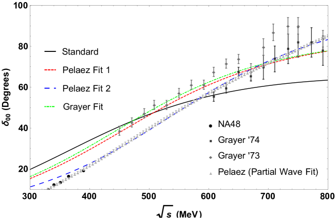
Figure 2: Partial wave fits to the $I=J=0$ scalar channel. References for the fit data are found in [3], whereas the standard values are found in [4].

Parameters	Grayer	Peláez 1	Peláez 2
$F\pm\Delta F\text{ (MeV)}$	63.16$\pm$1.62	65 (fixed)	75.98$\pm$ 0.16
$\mu\pm\Delta\mu\text{ (MeV)}$	1523.35$\pm$143.34	1607.89$\pm$3.62	2763.51 $\pm$ 23.81
$R^{2}$	0.9958	0.9951	0.9999

Table 1: Parameters for the Grayer and Peláez data fits and their respective coefficients of determination.

2.2 Finite-temperature Regime

The whole scattering process (taking into account effects of the thermal bath via the imaginary time formalism [7]) is given after building an effective thermal vertex that includes the contribution of all the powers of the tadpole $I_{\beta}=T^{2}/12$ that come from diagrams with 6 or more legs in the expanded metric (2). Taking this into account, we find an amplitude that reads as shown in the right side of Fig. 1, where $f(I_{\beta})=(1-I_{\beta}/F^{2})^{-1}$ is the thermal tadpole function and the loop integral $J(p;T)=J_{\epsilon}(\mu)+J_{fin}(p;T;\mu)$ has both zero and finite temperature contributions. We attain a proper renormalization of this quantity after redefining the vertices as

$$\frac{s}{(NF^{2})^{k+1}}\rightarrow\frac{s}{(NF^{2})^{k+1}}G_{0}^{\,k+1}(s),\,k=0,1,2,3,\cdots$$ (9)

Furthermore, we find that the renormalized coupling $G_{R}(s,\mu)$ reads the same as in the zero-temperature case. Thus, the finite-temperature renormalized amplitude reads

$$A_{R}(p;T)=\frac{sG_{R}(s;\mu)}{NF^{2}}\frac{f[G_{R}(s;\mu)I_{\beta}]}{1-\frac{sG_{R}(s;\mu)f[G_{R}(s;\mu)I_{\beta}]}{2F^{2}}J_{fin}(p;T;\mu)}.$$ (10)

3 The $f_{0}(500)$ Resonance and its Relationship with Chiral Symmetry Restoration

3.1 Thermal Unitarity

After replacing the partial wave expansion (8) into the the renormalized amplitude (10), we can extract the imaginary part as

$$\text{Im}\left[\frac{1}{a_{00}(s+i0^{+};T)}\right]=-\sigma_{T}(s,0),$$ (11)

where $\sigma_{T}(s,0)=1+2n(\sqrt{s}/2)$ (here $n(x)$ is the Bose-Einstein distribution) is the thermal phase space for massless pions. This means that unlike previous perturbative results [8], unitarity holds exactly in this framework.

3.2 Mass and Width of the $f_{0}(500)$ Resonance

Since unitarity was already checked, we can go to the second Riemann sheet and find the pole of $|a_{00}(s,T)|^{2}$; after doing this, we will have some insight about a symmetry-restoring behavior by studying the evolution with $T$ of the mass and the width of this resonance. We find a stronger evidence of this fact after obtaining the critical temperature and the critical exponent of the scalar susceptibility, whose $p=0$ limit is given as $\chi_{S}(T)\propto 1/\text{Re}\left\{s\right\}$ [9]. Its unitarized form is such that $\chi_{S}(T)/\chi_{S}(0)=\left[M_{p}^{2}(0)-\Gamma_{p}^{2}(0)/4\right]/\left[M_{p}^{2}(T)-\Gamma_{p}^{2}(T)/4\right]$, whose inverse is plotted in Fig. 3 along with the Inverse Amplitude Method result (IAM) [9] for massless pions.

Table 2 lists our main results for the critical temperatures and pole positions, as well as the critical exponents and coefficients of determination for $\chi_{S}(T)$ [3]. We can see that our $T=0$ masses and widths can be compared with those given for a phenomenological fit and that they lie between the well-known experimental bounds (see [3] for details).

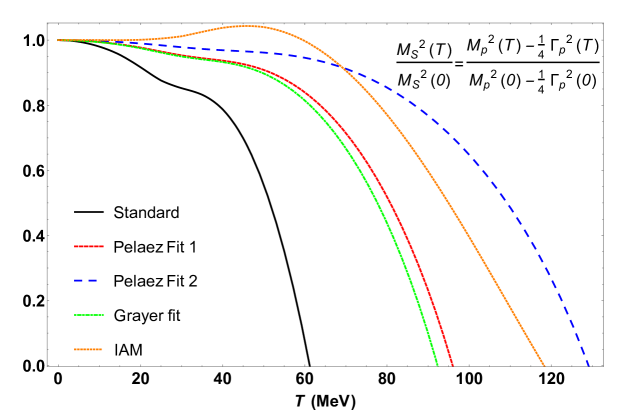
Figure 3: Inverse scalar susceptibility as function of the temperature for different parameter sets, along with the IAM result.

Fit	$T_{c}\text{ (MeV)}$	$M_{P}(0)\text{ (MeV)}$	$\Gamma_{P}(0)\text{ (MeV)}$	$\gamma_{\chi}$	$R^{2}_{\gamma_{\chi}}$
Grayer	92.33	438.81	536.47	0.875	0.99987
Peláez 1	96.00	452.42	546.26	0.938	0.99997
Peláez 2	129.07	535.53	534.59	0.919	0.99995
IAM	118.23	406.20	522.70	1.012	1
Standard	61.20	356.97	566.05	0.842	0.99728

Table 2: Pole positions, critical temperatures and exponents and coefficients of determination of $\chi_{S}(T)$ for the fits considered so far.

4 Conclusions

Although we work in the Chiral Limit, our analysis of ellastic pion scattering at finite temperature in the large-$N$ expansion grants a description of the $f_{0}(500)$ pole thermal dependence that is consistent with previous works [9]. Furthermore, the behavior of $\chi_{S}^{-1}(T)$ (saturated by the $f_{0}(500)$ pole) is consistent with a second-order phase transition, as seen in the lattice [2].

We have to point out that our $T_{c}$ results [3] are not far from the expected lattice values (about $\text{0.8}T_{\chi}$); besides, they are even closer to the result obtained for NJL-like models, i.e., $T_{c}\approx 100.7\text{ MeV}$ [10].

Our results for the critical exponents point out that they lie between the interval $\text{0.54}\leq\gamma_{\chi}\leq 1$, where the lower limit is given for an $O(4)$ three-dimensional Heisenberg model, and the upper limit is the exact result for a large-$N$ $O(N)$ four-dimensional nonlinear model (more details in [3]).

We acknowledge financial support by Spanish research projects FPA2014-53375-C2-2-P and FIS2014-5706-REDT; Santiago Cortés acknowledges Univ. de los Andes and COLCIENCIAS.

References

- [1] Y. Aoki, S. Borsanyi, S. Durr, Z. Fodor, S. D. Katz, S. Krieg and K. K. Szabo, JHEP 0906, 088 (2009).
- [2] A. Bazavov, T. Bhattacharya, M. Cheng, C. DeTar, H. T. Ding, S. Gottlieb, R. Gupta and P. Hegde et al., Phys. Rev. D 85, 054503 (2012).
- [3] S. Cortés, A. Gómez Nicola and J. Morales, Phys. Rev. D 93, 036001 (2016).
- [4] A. Dobado and J. Morales, Phys. Rev. D 52, 2878 (1995).
- [5] J. Gasser and H. Leutwyler, Annals Phys. 158, 142 (1984).
- [6] A. Dobado and J. R. Pelaez, Phys. Lett. B 286, 136 (1992).
- [7] M. Le Bellac, “Thermal Field Theory”. Cambridge University Press (1996).
- [8] A. Gomez Nicola, F. J. Llanes-Estrada and J. R. Pelaez, Phys. Lett. B 550, 55 (2002).
- [9] A. Gomez Nicola, J. Ruiz de Elvira and R. Torres Andres, Phys. Rev. D 88, 076007 (2013).
- [10] J. Berges, N. Tetradis and C. Wetterich, Phys. Rept. 363, 223 (2002).