Post Markovian Dynamics of Quantum Correlations: Entanglement vs. Discord

Abstract

Dynamics of an open two-qubit system is investigated in the post-Markovian regime, where the environments have a short-term memory. Each qubit is coupled to separate environment which is held in its own temperature. The inter-qubit interaction is modeled by XY-Heisenberg model in the presence of spin-orbit interaction and inhomogeneous magnetic field. The dynamical behavior of entanglement and discord has been considered. The results show that, quantum discord is more robust than quantum entanglement, during the evolution. Also the asymmetric feature of quantum discord can be monitored by introducing the asymmetries due to inhomogeneity of magnetic field and temperature difference between the reservoirs. By employing proper parameters of the model, it is possible to maintain non-vanishing quantum correlation at high degree of temperature. The results can provide a useful recipe for studying of dynamical behavior of two-qubit systems such as trapped spin-electrons in coupled quantum dots.

I INTRODUCTION

The weirdness of quantum mechanics lies on the concept of quantum correlation which is originated from the superposition principle. There are two important aspects of quantum correlation: quantum entanglement EPRPRA1935 ; SchrodingerNat1935 which is defined within the entanglement-separability paradigm and quantum discord ZurekPRL2001 ; HendersonJPA2001 , defined from an information-theoretic perspective. The quantitative and qualitative evaluation of such correlations is central task in conceptual studies of conceptual quantum mechanics, and it also has crucial significance in operative quantum information theory. A mixed state $\rho$ of a bipartite system is an entangled state if it not separable i.e. it can not prepared by Local Operation and Classical Communication (LOCC) tasks. There are many measures which evaluate the amount of entanglement of a quantum state. The entanglement of formation is one of these measures, which is enumerates the resources which is needed to create a given entangled state. For the case of a two-qubit bipartite system the formula of the entanglement of formation can be expressed as a smooth function of the concurrence and hence the concurrence can be take as a measure of entanglement in its own rightWoottersPRL1997 . The concurrence of the state $\rho_{AB}$ can be obtained explicitly as:

$$C(\rho_{AB})=\max\{0,2\lambda_{max}-\sum_{i=1}^{4}\,\lambda_{i}\},$$ (1)

where $\lambda_{i}$s are roots of the eigenvalues of the non-Hermitian matrix $R=\sqrt{\sqrt{\rho_{AB}}\tilde{\rho}_{AB}\sqrt{\rho_{AB}}}$, and $\tilde{\rho}_{AB}$ is defined by $\tilde{\rho}_{AB}:=(\sigma^{y}\otimes\sigma^{y})\rho_{AB}^{*}(\sigma^{y}\otimes\sigma^{y})$, here $\sigma^{y}$ is Pauli y-matrix WoottersPRL1997 .

Until some time ago, entanglement was considered as the only type of quantum correlation could be find in a composed quantum state. However, it has been discovered that some multi-partite separable states could speedup quantum computation algorithms KnillPRL1998 i.e. they possess some quantum features. Therefore, entanglement is not the only aspect of quantum correlation. Datta et. al. DattaPRL2008 have showen that the resource of this speedup is another important type of quantum correlations, named by Quantum Discord (QD). Quantum discord first introduced by Zurek et. al. ZurekPRL2001 and Henderson et. al. HendersonJPA2001 , independently in year 2001. The definition of QD lies on the difference between two classically equivalent definitions of mutual information in the quantum mechanics language. In mathematical sense the quantum discord could be obtained by eliminating the classical correlation from the total correlation measured by quantum mutual information. The classical correlation between the parts of a bipartite system can be obtained by use of the measurement-base conditional density operator. Hence we can write the discord with respect to the $B$ subsystem (right discord) as:

$$D_{B}(\rho_{AB})=I(\rho_{AB})-CC_{B}(\rho_{AB}).$$ (2)

Where $I(\rho_{AB})=S(\rho_{A})+S(\rho_{B})-S(\rho_{AB})$ is the mutual information and $CC_{B}(\rho_{AB})=\underset{\{\Pi_{k}^{(B)}\}}{\sup}\{S(\rho_{A})-S(\rho_{AB}|\{\Pi_{k}^{(B)}\})\}$ is the classical part of correlation. Here $\rho_{A(B)}$ and $\rho_{AB}$ refer to the reduced density matrix of subsystem $A(B)$ and the density matrix of the system as the whole and $S(\rho)=-Tr(\rho\,\log_{2}\rho)$ is Von Neumann entropy. The maximization in the definition of classical correlation is taken over the set of generalized measurements (POVMs) $\{\Pi_{k}^{(B)}\}$, and $S(\rho_{AB}|\{\Pi_{k}^{(B)}\})=\sum_{k=0}^{1}p_{k}S(\rho_{k})$ is the conditional entropy of subsystem $A$, with $\rho_{k}=Tr_{B}((I_{A}\otimes\Pi_{k}^{(B)})\,\>\rho_{AB}\,\>(I_{A}\otimes\Pi_{k}^{(B)}))/p_{k}$ and $p_{k}=Tr(\rho_{AB}\>(I_{A}\otimes\Pi_{k}^{(B)}))$. However, one can swap the role of the subsystems $A$ and $B$ to obtain discord with respect to $A$ subsystem (left discord), i.e. $D_{A}(\rho_{AB})$.

Decoherence is the main obstacle to preserving the superposition and hence quantum correlation in real quantum systems. Undesired leakage of the coherence of the system to the environment, due to unavoidable interaction between the quantum systems and their environment, leading to decoherence Schlosshauerbook2007 . Thermal decoherence plays a significant role to destroying the useful quantum correlation between the parts of the quantum systems. Although investigating the decohernce procedure in thermal equilibrium is useful but real systems are not in equilibrium VedralJP2009 and hence the dynamical behavior of the systems under non-equilibrium condition has to be elucidated. Furthermore, the formal analysis of an open quantum dynamics is considered in Markovian framework i.e. by assuming the weak system-environment coupling and the forgetful nature of the environmental system. Despite of its wide applicability, it should be kept in mind that Markovianity is only an approximation and the real physical systems may not fulfill these conditions. This imposes one to address the question of quantum feature survival in noisy as well as non-equilibrium conditions in the non-Markovian regime.

In propose to realize such systems we consider the non-equilibrium dynamics of a system including two coupled qubits in contact with different thermal baths. This is a system which is interesting both from theoretical and empirical point of view. Recent progresses in nano-technology provide the possibility of fabrication and manipulation of confined spins in nano-scale devices. Among these devices, semiconductor quantum dots becomes a useful device for manipulating, transferring and saving the quantum information. For example, data transferring between nuclear spins and electronic spins confined in a semiconductor quantum dot has been considered ReinaPRB2000 . These nuclear and the electronic are embedded in a solid state environment with huge degrees’ of freedom (bath). Because they interact with their bath in completely different manner, they experience different effects from environment. Nowadays, with the aid of NMR and quantum optical techniques, it is possible to change the temperature of the nuclear spins without affecting the electron spins temperature StepankoPRL2006 . A system consists of two spin-electron confined in two coupled quantum dotsLossPRA1998 ; DiVincenzoPRA1995 , is another example. In this system qubit is represented by a single spin-electron confined in each quantum dot. These qubits can be initialized, manipulated, and read out by extremely sensitive devices. In comparison with quantum optical and NMR systems, such systems are more scalable and more robust to the environmental affects. Each quantum dot could be coupled to different source and drain electrodes, during the fabrication process, and hence feels a different environment LegelPRB2007 .

In this paper, the non-equilibrium dynamics of an open quantum system is investigated. The system to be considered includes a two-qubit system interacting with surrounding environment. The inter-qubit separation is supposed large enough such that each qubit is embedded in a separate environment. The environments are modeled by thermal reservoirs (bosonic bathes) which are assumed to be in thermodynamic equilibrium in their own temperature $\beta_{i}=\frac{1}{k_{B}T_{i}}$. Furthermore each qubit is realized by the spin of an electron confined in a quantum dots, so due to weak lateral confinement, electrons can tunnel from one dot to the other and spin-spin and spin-orbit interactions between the two qubits exist. Also, it is assumed that an external magnetic field is applied to each quantum dot. Thus the inter-qubit interaction could be modeled by anisotropic XY Heisenberg system in the presence of the inhomogeneous magnetic field, equipped by spin-orbit interaction in the form of the Dzyaloshinski-Moriya (DM) interaction KavokinPRB2001 ; DzyaloshinskiJPCS1958 ; MoriyaPRL1960 . In the following, the influence of the parameters of the system (i.e. magnetic field (B), inhomogeneity of magnetic field (b), partial anisotropy($\chi$), mean coupling (J) and the spin-orbit interaction parameter (D)) and environmental parameters (i.e. temperatures $T_{1}$ and $T_{2}$ or equally $T_{M}$ and $\Delta T$, and the couplings strength $\gamma_{1}$ and $\gamma_{2}$) on the amount of entanglement and discord of the system is studied. The results show that the dynamics of quantum correlations depends on the geometry of connection, especially the geometry of connection can bold asymmetric property of quantum discord. Also the results show that, for an exponentially damping memory kernel, there is a steady state in asymptotically large time limit. The amount of both asymptotic entanglement and asymptotic discord decreases as the temperature increases but for asymptotic discord sudden death does not occur; asymptotic discord descends exponentially with temperature, while the entanglement suddenly vanishes above a critical temperature, $T_{M}^{cr.}$. The results also reveal that, the size of $T_{M}^{cr.}$ (temperature over which the quantum entanglement cease to exist) and the amount of both entanglement and discord can be improved by adjusting the value of the spin-orbit interaction parameter $D$. This parameter can be manipulated by adjusting the height of the barrier between two quantum dots.

The paper is organized as follows. In Sec. II, we introduce the Hamiltonian of the whole system-reservoir and then write the post-Markovian master equation governed on the system by tracing out the reservoirs’ degrees of freedom. Ultimately, for X-shaped initial states, the density matrix of the system at a later time is derived exactly. The effects of initial conditions and system parameters on the dynamics of entanglement and entanglement of asymptotic state of the system are presented in Sec. III. Finally in Sec. IV a discussion concludes the paper.

II THE MODEL AND HAMILTONIAN

A bipartite quantum system coupled to two reservoirs is described by the following Hamiltonian:

$$\hat{H}=\hat{H}_{S}+\hat{H}_{B1}+\hat{H}_{B2}+\hat{H}_{SB1}+\hat{H}_{SB2},$$ (3)

where $\hat{H}_{S}$ is the Hamiltonian of the system, $\hat{H}_{Bj}$ is the Hamiltonian of the jth reservoir $(j=1,2)$ and $\hat{H}_{SBj}$ denotes the interaction Hamiltonian of the system and jth reservoir. According to previous section, the system under consideration consists of two interacting spin electrons confined in two coupled quantum dots. Thus inter-qubit interaction includes spin-spin interaction and spin-orbit interaction (due to orbital motion of electrons). Such system could be described by a two-qubit anisotropic Heisenberg XY-model in the presence of an inhomogeneous magnetic field equipped by spin-orbit interaction with the following Hamiltonian (see HamidPRA2008 and references therein):

$$\hat{H}_{S}={\textstyle\frac{1}{2}}(J_{x}\,\sigma_{1}^{x}\sigma_{2}^{x}\,+J_{y}\,\sigma_{1}^{y}\sigma_{2}^{y}+\textbf{B}_{1}\cdot\boldsymbol{\sigma}_{1}+\textbf{B}_{2}\cdot\boldsymbol{\sigma}_{2}+\boldsymbol{D}.(\boldsymbol{\sigma}_{1}\times\boldsymbol{\sigma}_{2})),$$ (4)

where $\boldsymbol{\sigma}_{j}=(\sigma_{j}^{x},\sigma_{j}^{y},\sigma_{j}^{z})$ is the vector of Pauli matrices, $\textbf{B}_{j}\,(j=1,2)$ is the magnetic field on site j, $J_{\mu}s\,(\mu=x,y)$ are the real coupling coefficients (the interaction is anti-ferromagnetic (AFM) for $J_{\mu}>0$ and ferromagnetic (FM) for $J_{\mu}<0$) and $\boldsymbol{D}$ is Dzyaloshinski-Moriya term of spin-orbit interaction. Reparametrizing the above Hamiltonian with $\textbf{B}_{j}=B_{j}\,\hat{\boldsymbol{z}}$ such that $B_{1}=B+b$ and $B_{2}=B-b$, where b is magnetic field inhomogeneity, and $J:=\frac{J_{x}+J_{y}}{2}$, as the mean coupling coefficient in the XY-plane, $\chi:=\frac{J_{x}-J_{y}}{J_{x}+J_{y}}$, as partial anisotropy, $-1\leq\chi\leq 1$, and with the assumption $\boldsymbol{D}=J\,D\hat{\boldsymbol{\,z}}$ we have:

$$\hat{H}_{S} = J\chi(\sigma_{1}^{+}\sigma_{2}^{+}+\sigma_{1}^{-}\sigma_{2}^{-})+J(1+i\,D)\,\sigma_{1}^{+}\sigma_{2}^{-}+J(1-i\,D)\,\sigma_{1}^{-}\sigma_{2}^{+}$$ (5)

$$+ (\frac{{B+b}}{2})\sigma_{1}^{z}+(\frac{{B-b}}{2})\sigma_{2}^{z},$$

where $\sigma^{\pm}=\frac{1}{2}(\sigma^{x}\pm i\sigma^{y})$, denote the lowering and raising operators. The spectrum of $\hat{H}_{S}$, in the standard basis $\{|00\rangle,|01\rangle,|10\rangle,|11\rangle\}$, is easily obtained as

$$\begin{array}[]{l}|\varepsilon_{1,2}\rangle=|\Psi^{\pm}\rangle=\sin\theta_{\pm}e^{i\phi}|01\rangle+\cos\theta_{\pm}|10\rangle\,,\,\;\;\;\;\varepsilon_{1,2}=\pm\xi\,,\\ \\ |\varepsilon_{3,4}\rangle=|\Sigma^{\pm}\rangle=\sin\theta^{\prime}_{\pm}|00\rangle+\cos\theta^{\prime}_{\pm}|11\rangle\,,\,\;\;\;\;\;\;\;\varepsilon_{3,4}=\pm\eta\,.\end{array}$$ (9)

Where $\tan\theta_{\pm}=\sqrt{\pm(\frac{\xi\pm b}{\xi\mp b})}$, $\tan\phi=D$ and $\tan\theta^{\prime}_{\pm}=\sqrt{\pm(\frac{\eta\pm B}{\eta\mp B})}$ with $\xi=(b^{2}+J^{2}(1+D^{2}))^{1/2}$ and $\eta=(B^{2}+(J\chi)^{2})^{1/2}$. The Hamiltonian of the reservoir coupled to jth spin are given by

$$\hat{H}_{Bj}=\sum_{n}\omega_{n}\hat{a}_{nj}^{{\dagger}}\hat{a}_{nj}\,,$$ (10)

where $\hat{a}_{nj}^{{\dagger}}$ and $\hat{a}_{nj}$ are the creation and the annihilation operators of the jth bath mode, respectively. In the full dissipative regime and in the absence of dephasing processes the interaction between the system and the jth bath is governed by the following HamiltonianHamidEPJD2010 :

$$\hat{H}_{SBj}=(\sigma_{j}^{+}+\sigma_{j}^{-})(\sum_{n}g_{n}^{(j)}\hat{a}_{n,\,j}+g_{n}^{(j)*}\hat{a}_{n,\,j}^{{\dagger}})=\sum_{\mu}(\hat{\Lambda}{}_{j,\,\mu}^{+}+\hat{\Lambda}{}_{j,\,\mu}^{-})(\hat{G}_{j,\,\mu}+\hat{G}_{j,\,\mu}^{\dagger}),$$ (11)

The system operators $\hat{\Lambda}_{j,\,\mu}^{\pm}$ are chosen to satisfy $[\hat{H}_{S},\hat{\Lambda}_{j,\,\mu}^{\pm}]=\pm\omega_{j,\,\mu}\hat{\Lambda}_{j,\,\mu}^{\pm}$, and the $\textit{\^{G}}_{j,\,\mu}$’s are the random operators of reservoirs and act on the bath degrees of freedom. The Greek letter indexes are related to the transitions between the internal levels of the system induced by the bath. The irreversibility hypothesis implies that the evolution of the system does not influence the states of the reservoirs and the state of whole system+reservoirs is describing by, $\hat{\sigma}(t)=\hat{\rho}(t)\hat{\rho}_{B1}(0)\hat{\rho}_{B2}(0)$, where $\hat{\rho}(t)$ is the reduced density matrix describing the system and each bath is supposed to be in their thermal state at temperature $T_{j}=\frac{1}{\beta_{j}}$, i.e. $\hat{\rho}_{Bj}=\emph{e}^{-\beta_{j}\hat{H}_{Bj}}/Z$, where $Z=Tr(\emph{e}^{-\beta_{j}\hat{H}_{Bj}})$ is the partition function of the jth bath. Dynamics of the reduced density matrix of system in the Post-Markov approximation is describing with the following master equationShabaniPRA2005 ; DieterichNat2015 ; CampbellPRA2012 ; BudiniPRE2014 ; Sinaysky :

$$\frac{d\hat{\rho}}{dt}=-i[\hat{H}_{S},\hat{\rho}]+\mathcal{L}\int_{0}^{t}dt^{\prime}[k(t^{\prime})\exp(\mathcal{L}\,t^{\prime})\hat{\rho}(t-t^{\prime})],$$ (12)

where $\mathcal{L}=\mathcal{L}_{1}+\mathcal{L}_{2}$ and $\mathcal{L}_{j}(\hat{\rho})\,(j=1,2)$ is dissipator or Lindbladian given by

$$\mathcal{L}_{j}(\hat{\rho})\equiv\sum_{\mu,\,\nu}J_{\mu,\,\nu}^{(j)}(\omega_{j,\,\nu})\{[\hat{\Lambda}_{j,\,\mu}^{+},[\hat{\Lambda}_{j,\,\nu}^{-},\hat{\rho}]]-(1-\emph{e}^{\beta_{j}\omega_{j,\,\nu}})[\hat{\Lambda}_{j,\,\mu}^{+},\hat{\Lambda}_{j,\,\nu}^{-}\hat{\rho}]\}.$$ (13)

Here $J_{\mu,\nu}^{(j)}(\omega_{j,\nu})$ is the spectral density of the jth reservoir given by:

$$J_{\mu,\,\nu}^{(j)}(\omega_{j,\,\nu})=\int_{0}^{\infty}d\tau\emph{e}^{i\omega_{j,\,\nu}\tau}\langle\textit{\={G}}_{j,\,\mu}(\tau)\,\,\textit{\^{G}}_{j,\,\nu}\rangle_{\rho_{Bj}},$$ (14)

with $\textit{\={G}}_{j,\,\nu}(\tau)=\emph{e}^{-iH_{Bj}\tau}\textit{\^{G}}_{j,\,\mu}^{\,\,\,{\dagger}}\emph{e}^{iH_{Bj}\tau}$. For the bosonic thermal bath modeled by an infinite set of harmonic oscillators, the Weisskpof-Wignner-like approximation implies that: $J^{(j)}(\omega_{\mu})=\gamma_{j}(\omega_{\mu})n_{j}(\omega_{\mu})$ with the property of $J^{(j)}(-\omega_{\mu})=\emph{e}^{\beta_{j}\omega_{\mu}}J^{(j)}(\omega_{\mu})$, where $n_{j}(\omega_{\mu})=(\emph{e}^{\beta_{j}\omega_{\mu}}-1)^{-1}$ is the thermal mean value of the number of excitation in the $j$th reservoir at frequency $\omega_{\mu}$ and $\gamma_{j}(\omega_{\mu})$ is the coupling coefficient of system and the $j$th reservoir. Thus, we can write:

$$\mathcal{L}_{j}(\hat{\rho}) = \sum_{\mu=1}^{4}J^{(j)}(-\omega_{\mu})(2\hat{\Lambda}_{j,\,\mu}^{+}\hat{\rho}\hat{\Lambda}_{j,\,\mu}^{-}-\{\hat{\rho},\hat{\Lambda}_{j,\,\mu}^{-}\hat{\Lambda}_{j,\,\mu}^{+}\}_{+}))$$ (15)

$$+ \sum_{\mu=1}^{4}J^{(j)}(\omega_{\mu})(2\hat{\Lambda}_{j,\,\mu}^{-}\hat{\rho}\hat{\Lambda}_{j,\,\mu}^{+}-\{\hat{\rho},\hat{\Lambda}_{j,\,\mu}^{+}\hat{\Lambda}_{j,\,\mu}^{-}\}_{+})),$$

with the transition frequencies

$$\omega_{1}=\xi-\eta=-\omega_{4},\,\,\,\,\,\,\,\,\,\,\,\,\,\,\,\ \omega_{2}=\xi+\eta=-\omega_{3},$$ (16)

and the transition operators

$$\hat{\Lambda}_{j,\,1}^{+} = c_{j,\,1}|\Psi^{+}\rangle\langle\Sigma^{+}|,\,\,\,\,\,\,\,\,\,\,\,\,\,\,\,\,\,\,\,\,\,\,\ \hat{\Lambda}_{j,\,2}^{+}=c_{j,\,2}|\Psi^{+}\rangle\langle\Sigma^{-}|,$$

$$\hat{\Lambda}_{j,\,3}^{+} = c_{j,\,3}|\Psi^{-}\rangle\langle\Sigma^{+}|,\,\,\,\,\,\,\,\,\,\,\,\,\,\,\,\,\,\,\,\,\,\,\ \hat{\Lambda}_{j,\,4}^{+}=c_{j,\,4}|\Psi^{-}\rangle\langle\Sigma^{-}|,$$ (17)

where

$$\mid c_{j,\,1}\mid^{2} = \mid c_{j,\,4}\mid^{2}=\frac{1}{2\xi\eta}(\xi\eta+J^{2}\chi+(-1)^{j}Bb),$$

$$\mid c_{j,\,2}\mid^{2} = \mid c_{j,\,3}\mid^{2}=\frac{1}{2\xi\eta}(\xi\eta-J^{2}\chi-(-1)^{j}Bb),$$ (18)

and $\hat{\Lambda}_{j,\,\mu}^{-}=(\hat{\Lambda}_{j,\,\mu}^{+})^{\dagger}$. Note that, the transition operators $\hat{\Lambda}_{j,\,\mu}^{\pm}$ defined in Eq. (17) just describe the energy exchange between the system and environment (dissipative coupling), including both excitation and de-excitation of the qubits. The absence of the transitions $\Sigma^{+}\leftrightarrow\Sigma^{-}$ and $\Psi^{+}\leftrightarrow\Psi^{-}$ stems in the omittance of the dephasing processes in the system-bath interaction Hamiltonian. In addition in the rest of the paper, the non-dispersive coupling coefficient is considered i.e. $\gamma_{j}(\omega_{\mu})=\gamma_{j}$.

An analytical solution of master equation (12) can be obtained by solving the eigenvalue equation $\mathcal{L}\rho=\lambda\rho$. In this order, the Lindblad superoperator diagonalized with the aid of its Jordan decomposition form $J$ with $\mathcal{L}=SJS^{-1}$. Fortunately, the master integro-differential equation (12) has an important property, when the spectrum of $\hat{H}_{s}$ (see eq.(9)) is non-degenerate, the equations for diagonal elements of density matrix decouple from non-diagonal ones Breuerbook2002 . Thus for the case $\xi\neq\eta$, where the spectrum (9) is not degenerate, we can consider them separately. The Lindbladian for diagonal terms can be written as a time independent $4\times 4$ matrix in the energy basis $\{|\varepsilon_{i}\rangle\}_{i=1}^{4}$:

$$\mathcal{L}^{diag}=\left({\begin{array}[]{cccc}-(X_{1}^{-}+Y_{2}^{-})&0&X_{1}^{+}&Y_{2}^{+}\\ 0&-(X_{1}^{+}+Y_{2}^{+})&Y_{2}^{-}&X_{1}^{-}\\ X_{1}^{-}&Y_{2}^{+}&-(X_{1}^{+}+Y_{2}^{-})&0\\ Y_{2}^{-}&X_{1}^{+}&0&-(X_{1}^{-}+Y_{2}^{+})\end{array}}\right),$$ (23)

where

$$X_{\mu}^{\pm}=2\sum_{j=1,2}J^{(j)}(\mp\omega_{\mu})\mid a_{j,\,1}\mid^{2},$$

$$Y_{\mu}^{\pm}=2\sum_{j=1,2}J^{(j)}(\mp\omega_{\mu})\mid a_{j,\,2}\mid^{2}.$$ (24)

The Jordan form of this matrix can be obtained easily as:

$$\mathcal{L}^{diag}=SJ^{(d)}S^{-1},$$

with

$$S=\left({\begin{array}[]{cccc}\frac{Y_{2}^{+}}{Y_{2}^{-}}&\frac{Y_{2}^{+}}{Y_{2}^{-}}&-1&-1\\ \frac{X_{1}^{-}}{X_{1}^{+}}&-1&\frac{X_{1}^{-}}{X_{1}^{+}}&-1\\ \frac{X_{1}^{-}}{X_{1}^{+}}\frac{Y_{2}^{+}}{Y_{2}^{-}}&-\frac{Y_{2}^{+}}{Y_{2}^{-}}&-\frac{X_{1}^{-}}{X_{1}^{+}}&1\\ 1&1&1&1\end{array}}\right),$$

and

$$J^{(d)}=diag[J_{11}^{(d)}=0,J_{22}^{(d)}=-X_{1},J_{33}^{(d)}=-Y_{2},J_{44}^{(d)}=-(X_{1}+Y_{2})].$$

Knowing the eigenvalues of Linbladian superoperator, $\lambda_{i}^{(d)}=J_{ii}^{d}$ and the memory kernel $k(t)$, the function $\xi_{i}^{(d)}(t)=\xi(\lambda_{i}^{(d)},t)=Lap^{-1}[\frac{1}{s-\lambda_{i}^{(d)}k(s-\lambda_{i}^{(d)})}]$ can be calculated. Thus the solution of the master equation yields the diagonal elements of the density matrix in the energy basis as:

$$R(t)=S\,diag(\xi(J_{11}^{(d)},t),\xi(J_{22}^{(d)},t),\xi(J_{33}^{(d)},t),\xi(J_{44}^{(d)},t))\,S^{-1}R(0)=P(t)\,R(0),$$

where $R(t)=(\rho_{11}(t),\rho_{22}(t),\rho_{33}(t),\rho_{44}(t))^{T}$. In the energy basis, the Lindbladian corresponding to the non-diagonal elements in master equation (12) is in Jordan( diagonal) form:

$$\mathcal{L}^{nondiag}=J^{(n)}=diag(J_{11}^{(n)},J_{22}^{(n)},J_{33}^{(n)},J_{44}^{(n)})=diag(-2i\xi,2i\xi,-2i\eta,2i\eta)-\mbox{$\textstyle\frac{1}{2}$}(X_{1}+Y_{2})I,$$

where $I$ denotes a $4\times 4$ identity matrix. Thus the eigenvalues of Lindbladian of non-diagonal elements is determined as $\lambda_{i}^{(n)}=J_{ii}^{(n)}$ and hence the function $\xi_{i}^{(n)}(t)=\xi(J_{ii}^{(n)},t)=Lap^{-1}[\frac{1}{s-J_{ii}^{(n)}k(s-J_{ii}^{(n)})}]$ can be obtained. The non-diagonal elements of density matrix in the later time and in the energy basis can be calculated as:

$$Q(t)=diag(\xi(J_{11}^{(n)},t),\xi(J_{22}^{(n)},t),\xi(J_{33}^{(n)},t),\xi(J_{44}^{(n)},t))\,Q(0),$$

with $Q(t)=(\rho_{12}(t),\rho_{21}(t),\rho_{34}(t),\rho_{43}(t))^{T}$.

Now, the dynamics of reduced density operator of system is determined if the memory function (kernel) is determined. In the following we assume an exponentially damping function for the kernel with the form:

$$k(t)=\gamma_{0}e^{-\gamma_{0}t},$$ (26)

where $\gamma_{0}^{-1}$ denotes the characteristic time of the environment’s memory function (also called “coarse-graining time”). Therefore we have $\xi(\lambda_{i},t)=\frac{\gamma_{0}e^{\lambda_{i}t}+\lambda_{i}e^{-\gamma_{0}t}}{\lambda_{i}+\gamma_{0}}.$ Consequently, the diagonal terms of density matrix in the energy basis can be obtained as:

$$\rho_{i\,i}(t)=\sum_{j=1}^{4}p_{i\,j}\,\rho_{j\,j}(0),$$ (27)

where $p_{ij}$ are elements of matrix $P(t)=[p_{ij}]_{4\times 4}$ and are given in the appendix A, explicitly. The non-diagonal element of density matrix in the energy basis can be written as:

$$\,\rho_{1\,2}(t)=\frac{e^{-t\gamma_{0}}\left(X_{1}+Y_{2}-2(e^{-\mbox{$\textstyle\frac{1}{2}$}t(X_{1}+Y_{2}-2(\gamma_{0}-2i\xi))}\gamma_{0}-2i\xi)\right)}{X_{1}+Y_{2}-2(\gamma_{0}-2i\xi)}\rho_{1\,2}(0),\,\,\,\,\,\,\,\,\rho_{2\,1}(t)=\rho_{1\,2}^{*}(t),$$

$$\rho_{3\,4}(t)=\frac{e^{-t\gamma_{0}}\left(X_{1}+Y_{2}-2(e^{-\mbox{$\textstyle\frac{1}{2}$}t(X_{1}+Y_{2}-2(\gamma_{0}-2i\eta))}\gamma_{0}-2i\eta)\right)}{X_{1}+Y_{2}-2(\gamma_{0}-2i\eta)}\rho_{3\,4}(0),\,\,\,\,\,\,\,\,\rho_{4\,3}(t)=\rho_{3\,4}^{*}(t).$$ (28)

The spectrum (9)becomes degenerate at $\xi=\eta$, for which the above solution is not valid. The state of the system is not well defined at this critical point. This critical point assigns a critical value for the parameters of the system such as critical magnetic field ($B_{c}$), critical parameter of inhomogeneity of magnetic field ($b_{c}$), critical spin-orbit interaction parameter ($D_{c}$) and etc. Indeed quantum phase transition may be occurs at this critical point and hence the amounts of quantum correlation of the system changes abruptly when the parameters cross their critical values. The behavior of thermal entanglement at this point is studied in HamidPRA2008 . For the case of memory-less evolution i.e. $k(t)=\delta(t)$ or $\gamma\rightarrow 0$ and also for the asymptotic large times i.e. $t\rightarrow\infty$ the evolution reduce to the Markovian case.

Asymptotic case

The decoherence induced by environments does not prevent the creation of a steady state level of quantum correlation, regardless of the initial state of the system. Due to Eq. (26) the effects of memory decrease by time and hence the evolution becomes Markovian, at the large time limit. At the large time limit, the non-diagonal elements (II) vanish and $\hat{\rho}(t)$ converges to a diagonal density matrix (in the energy basis):

$$\hat{\rho}^{\infty}=\hat{\rho}_{asymptotic}=\lim_{t\rightarrow\infty}\hat{\rho}(t)=\frac{1}{X_{1}Y_{2}}\,\,\,\textrm{diagonal}(X_{1}^{+}Y_{2}^{+},X_{1}^{-}Y_{2}^{-},X_{1}^{-}Y_{2}^{+},X_{1}^{+}Y_{2}^{-}),$$ (29)

which is time independent. Therefore, there is a stationary state which the system tends asymptotically. This asymptotic state is independent on the initial conditions due to forgetful treatment of environment in the Markovian regime. There is an interesting limiting case for which the coupled quantum dots are in contact with the reservoirs at identical temperatures ($\beta_{1}=\beta_{2}=\beta$). In this case, it is easy to show that the reduced density matrix $\hat{\rho}^{\infty}$ takes the thermodynamic canonical form for a system described by the Hamiltonian $\hat{H}_{S}$ at temperature $T=\beta^{-1}$ i.e. $\hat{\rho}^{\infty}(\Delta T=0)\equiv\hat{\rho}_{T}=\frac{e^{-\beta H_{S}}}{Z}$, where $Z=Tr(e^{-\beta H_{S}})$ is the partition function. Thermal entanglement and thermal discord properties of such systems have been studied substantially in Refs. HamidPRA2008 ; WerlangPRA2010 , respectively.

III Results and Discussion

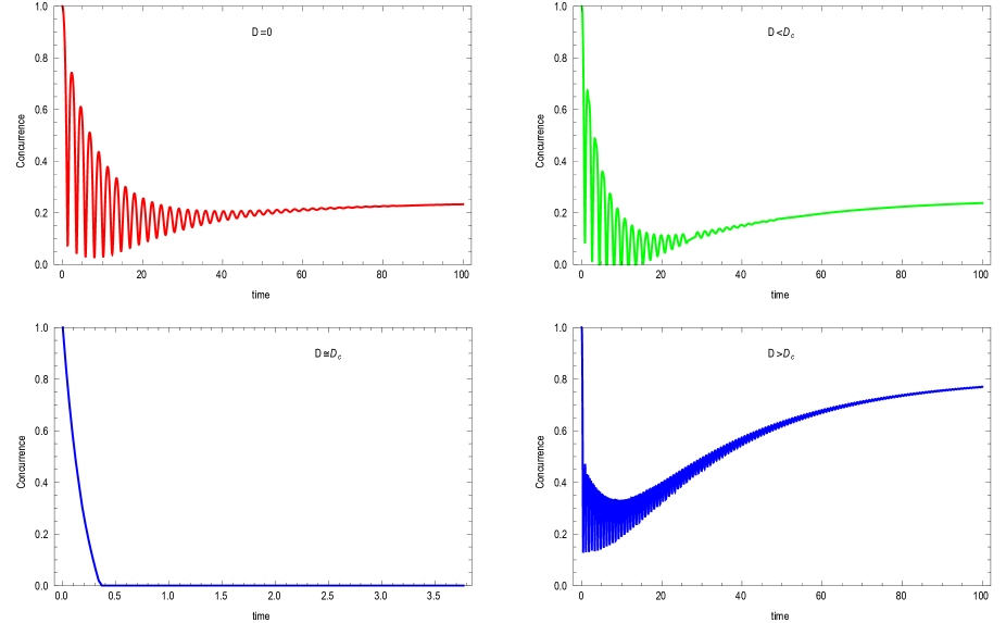
Figure 1: (Color online): Dynamical behavior of the concurrence for a maximally entangled initial state for different values of $D$ around $D_{c}\approx 1.68$. Here $J=1$, $\chi=0.9$, $B=2$, $b=1$, $T_{1}=1.25$, $T_{2}=0.75$ and $\frac{\gamma_{0}}{\bar{\gamma}}=200$. All parameters are dimensionless.

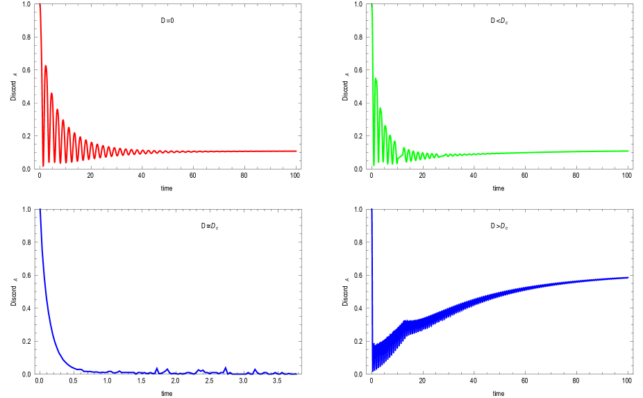
Figure 2: (Color online): Dynamical behavior of the left discord for a maximally entangled initial state for different values of $D$ around $D_{c}\approx 1.68$. Here $J=1$, $\chi=0.9$, $B=2$, $b=1$, $T_{1}=1.25$, $T_{2}=0.75$ and $\frac{\gamma_{0}}{\bar{\gamma}}=200$. All parameters are dimensionless.

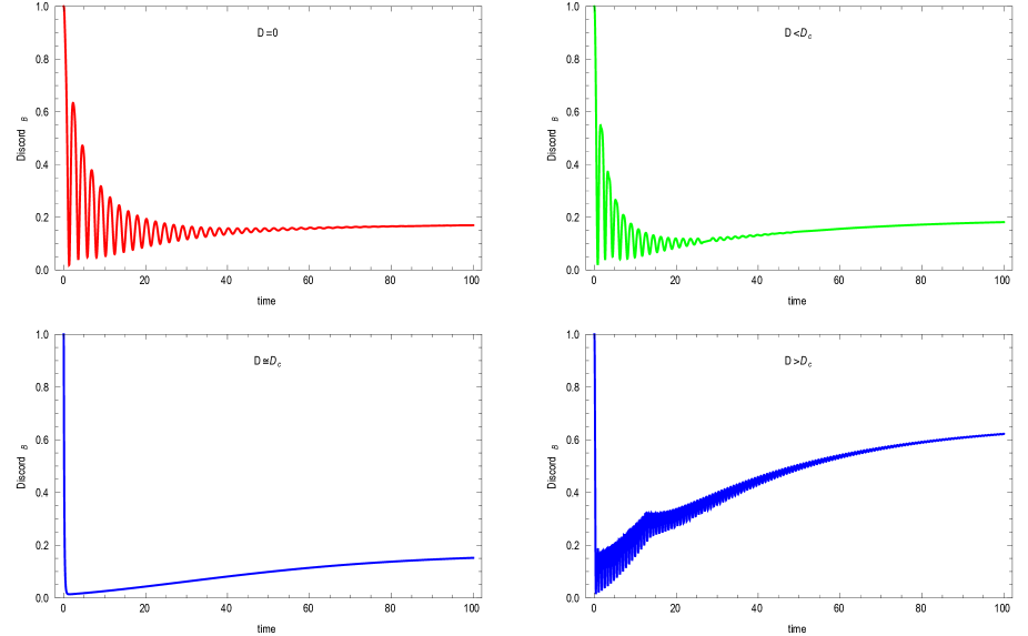
Figure 3: (Color online): Dynamical behavior of the right discord for a maximally entangled initial state for different values of $D$ around $D_{c}\approx 1.68$. Here $J=1$, $\chi=0.9$, $B=2$, $b=1$, $T_{1}=1.25$, $T_{2}=0.75$ and $\frac{\gamma_{0}}{\bar{\gamma}}=200$. All parameters are dimensionless.

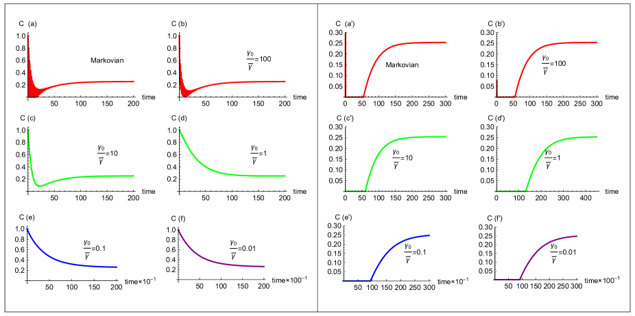
Figure 4: (Color online): Dynamics of the concurrence for different values of $\frac{\gamma_{0}}{\bar{\gamma}}$ when system is initially in a maximally entangled state (left graphs) and a non zero-discord separable state (right graphs). Here $J=1$, $\chi=0.9$, $B=2$, $b=1$, $D=1$, $T_{1}=1.25$ and $T_{2}=0.75$. All parameters are dimensionless.

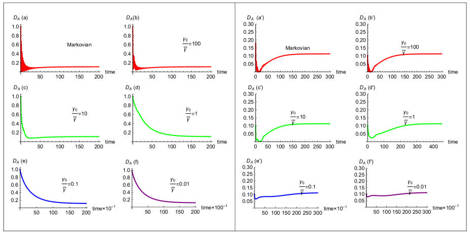
Figure 5: (Color online): Dynamics the left discord for different values of $\frac{\gamma_{0}}{\bar{\gamma}}$ when system is initially in a maximally entangled state (left graphs) and a non zero-discord separable state (right graphs). Here $J=1$, $\chi=0.9$, $B=2$, $b=1$, $D=1$, $T_{1}=1.25$ and $T_{2}=0.75$. All parameters are dimensionless.

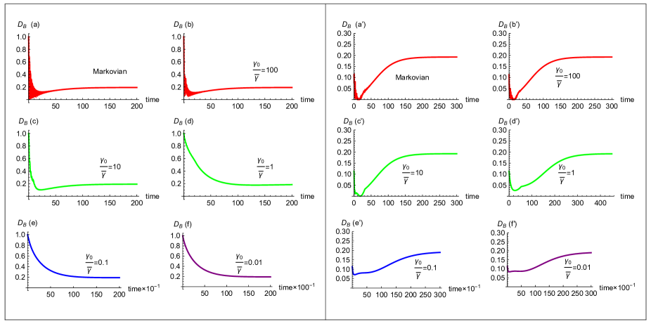
Figure 6: (Color online): Dynamics of the right discord for different values of $\frac{\gamma_{0}}{\bar{\gamma}}$ when system is initially in a maximally entangled state (left graphs) and a non zero-discord separable state (right graphs). Here $J=1$, $\chi=0.9$, $B=2$, $b=1$, $D=1$, $T_{1}=1.25$ and $T_{2}=0.75$. All parameters are dimensionless.

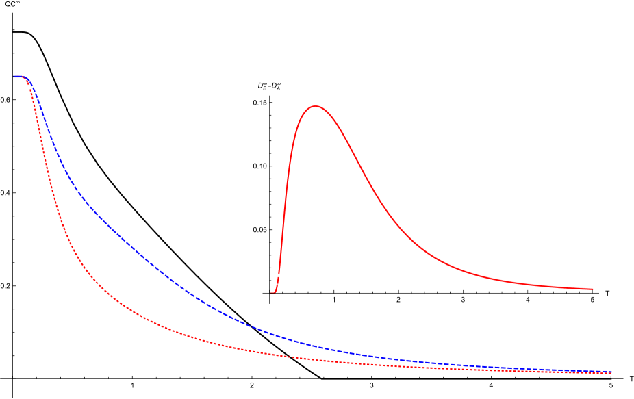
Figure 7: (Color online): (Color online) The asymptotic concurrence (black solid line), the asymptotic left discord (red dotted line) and the asymptotic  right discord (blue dashed line) vs. temperature, $T=T_{1}=T_{2}$. Inset : $D_{B}^{\infty}-D_{A}^{\infty}$ vs. $T$. Here $J=1$, $\chi=0.9$, $B=b=2$ and $D=2$. All parameters are dimensionless.

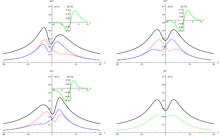
Figure 8: (Color online): Influence of geometry of connection on the asymptotic quantum correlations : the asymptotic concurrence (black solid line), the asymptotic left discord (red dotted line) and the asymptotic right discord (blue dashed line). Insets : $D_{B}^{\infty}-D_{A}^{\infty}$ vs. b for different values of $\Delta T$. The last graph depicts the behavior of the asymptotic concurrence (black solid line) and the averaged asymptotic discord ($\frac{D_{B}^{\infty}+D_{A}^{\infty}}{2}$) (green dot-dashed line) vs. $b$ in the thermal equilibrium condition. Here $J=1$, $\chi=0.9$, $B=2$ and $D=2$. All parameters are dimensionless.

Knowing the density matrix, one can calculate the concurrence, as a measure of entanglement and the quantum discord, as a measure of quantum correlation. Evidently, the results depend on the parameters involved. This prevents one from writing an analytic expression for the concurrence and/or the discord, but it is possible to calculate them for a given set of the parameters. Influence of a parameter on the dynamical and asymptotical behavior of quantum correlations could be studied by drawing their variation versus the mentioned parameter when the other parameters are fixed. The results are depicted in Figures 1-8. Figs. 1-6 compare the time evolution of the concurrence and the quantum discord and Figs.7 and 8 depict the asymptotic concurrence and quantum discord versus the system and environment parameters. The results of Figs. 1-6 show that all type of considered quantum correlations reach a steady value after some coherent oscillations. These coherent oscillations, are due to competition of the unitary and dissipative terms in master equation (12). Due to the kernel (26), the environment losses its memory during the evolution and hence the dynamics tends to the Markovian case at asymptotically large time limit. Figures 1-3 depict influence of spin-orbit parameter, $D$ on the post-Markovian dynamics of the concurrence, left and right discord, respectively for maximally entangled initial state $|\psi^{+}\rangle=\frac{1}{\sqrt{2}}(|01\rangle+|10\rangle)$. The results show that increasing $D$ improves the amount of steady state quantum correlation. Figures 4-6 show the dynamics of concurrence, left and right discord, respectively in different dynamical regimes for maximally entangled and also for non zero-discord separable initial states. The results show that the initial coherent oscillations are indicator of Markovianity of evolution and disappear in non-Markovian regime and also steady state level of quantum correlation achieves at earlier time for Markovian case. Figure 7 illustrates the asymptotic quantum correlation vs. temperature when two bathes are held in the same temperature. This figure reveals that the asymptotic entanglement vanishes above a critical temperature (entanglement sudden death). But quantum discord sudden death does not never occurs. This is due to the fact that the set of zero-discord states has no volume in the state space i.e. almost all quantum states possess quantum discord FerraroPRA2010 . Since each qubit experiences different magnetic fields, the symmetry of asymptotic right and left discords breaks for $T\geq 0$. Variation of the asymptotic quantum correlation is depicted in figure 8 for differnt ways of connections. Because each qubit is held in its own temperature and experiences different magnetic field, there are two different ways for connecting the quantum dots to their bathes HamidEPJD2010 : (i) "direct geometry"; where a high temperature bath couples to the quantum dots which is in the stronger magnetic field i.e. $b\Delta T>0$ and (ii) "indirect geometry"; where a high temperature bath couples to the quantum dot which is in the weaker magnetic field i.e. $b\Delta T<0$. The results show that inhomogeneity of magnetic field removes the degeneracy of left and right discord and the amount of this symmetry breaking depends on the temperature difference between bathes. This figure reveals that, if the measurement performed on the qubit which is in the stronger magnetic field, higher amount of asymptotic quantum discord could be achieved. So, the geometry of connection determines the amount of asymptotic quantum correlation an hence is important.

IV Conclusion

The Dynamics of non-equilibrium thermal entanglement and thermal discord of an open two-qubit system is investigated. The inter-qubit interaction is considered as the Heisenberg interaction in the presence of inhomogeneous magnetic field and spin-orbit interaction, raised from the Dzyaloshinski- Moriya (DM) anisotropic anti-symmetric interaction. Each qubit interacts with a separate thermal reservoir which is held in its own temperature. For physical realization of the model we address to the spin states of two electrons which are confined in two coupled quantum dots, respectively. The dots are assumed to biased via different sources and drains and hence experience different environments. The effects of the parameters of the model, including the parameters of the system (especially, the parameter of the spin-orbit interaction, $D$, and magnetic field inhomogeneity, $b$) and environmental parameters (particularly, mean temperature $T_{M}$ and temperature difference $\Delta T$), on the dynamics of the system is investigated, by solving the quantum Markov-Born master equation of the system. Tracing the dynamics of the system allowed us to distinguish between the quantum correlation produced by the inter-qubit interaction and/or by the environment. Decoherence induced by thermal bathes are competing with inter-qubit interaction terms leading to the system evolves to an asymptotic steady state. The size of the entanglement and discord of this steady state and also the dynamical behavior of the entanglement depend on the parameters of the model and also on the geometry of connection. The results reveal that increasing the size of DM interaction, $D$, enhances the amount of all asymptotic quantum correlation measures. Also the results show that the asymptotic entanglement of the system dies above a critical temperature $T_{cr.}$ and entanglement sudden death occurs. The size of $T_{cr.}$ and the amount of asymptotic entanglement can be enhanced by choosing a suitable value of $D$ and the temperature difference $\Delta T$. On the other hand the results show that thermal discord could live in higher temperatures than thermal entanglement and quantum discord sudden death does not occurs. Also, introducing magnetic field inhomogeneity breaks the symmetry between left and right discord. The results show that if the magnetic field applied on right(left) qubit is greater then the size of right(left) discord is higher. Furthermore, we find that choosing proper geometry of connection is important for creating and maintaining the quantum correlation.

Appendix A elements of marix P

The elements of matrix $P(t)=[p_{ij}]_{4\times 4}$ in the equation (27) can be written as follow:

$$p_{1\,1} = \frac{1}{X_{1}Y_{2}}[\frac{X_{1}^{-}Y_{2}^{+}(e^{-t\gamma_{0}}X_{1}-e^{-tX_{1}}\gamma_{0})}{X_{1}-\gamma_{0}}+\frac{X_{1}^{+}Y_{2}^{-}\left(e^{-t\gamma_{0}}Y_{2}-e^{-tY_{2}}\gamma_{0}\right)}{Y_{2}-\gamma_{0}}$$

$$+ \frac{e^{-t\gamma_{0}}X_{1}^{-}Y_{2}^{-}\left(X_{1}+Y_{2}-e^{-t\left(X_{1}+Y_{2}-\gamma_{0}\right)}\gamma_{0}\right)}{X_{1}+Y_{2}-\gamma_{0}}+X_{1}^{+}Y_{2}^{+}],$$

$$p_{1\,2} = \frac{X_{1}^{+}Y_{2}^{+}}{X_{1}Y_{2}}[\frac{e^{-t\gamma_{0}}X_{1}Y_{2}(X_{1}+Y_{2}-2\gamma_{0})}{(X_{1}-\gamma_{0})(X_{1}+Y_{2}-\gamma_{0})(\gamma_{0}-Y_{2})}+\frac{e^{-tX_{1}}\gamma_{0}}{X_{1}-\gamma_{0}}+\frac{e^{-tY_{2}}\gamma_{0}}{Y_{2}-\gamma_{0}}$$

$$- \frac{e^{-t(X_{1}+Y_{2})}\gamma_{0}}{X_{1}+Y_{2}-\gamma_{0}}+1]$$

$$p_{1\,3} = \frac{X_{1}^{+}}{X_{1}Y_{2}}[-\frac{\left(e^{-tX_{1}}\gamma_{0}-e^{-t\gamma_{0}}X_{1}\right)Y_{2}^{+}}{\gamma_{0}-X_{1}}+\frac{Y_{2}^{-}\left(e^{-tY_{2}}\gamma_{0}-e^{-t\gamma_{0}}Y_{2}\right)}{\gamma_{0}-Y_{2}}$$

$$+ \frac{e^{-t\gamma_{0}}Y_{2}^{-}\left(X_{1}+Y_{2}-e^{-t(X_{1}+Y_{2}-\gamma_{0})}\gamma_{0}\right)}{-X_{1}-Y_{2}+\gamma_{0}}+Y_{2}^{+}],$$

$$p_{1\,4} = \frac{Y_{2}^{+}}{X_{1}Y_{2}}[-\frac{\left(e^{-tY_{2}}\gamma_{0}-e^{-t\gamma_{0}}Y_{2}\right)X_{1}^{+}}{\gamma_{0}-Y_{2}}+\frac{X_{1}^{-}\left(e^{-tX_{1}}\gamma_{0}-e^{-t\gamma_{0}}X_{1}\right)}{\gamma_{0}-X_{1}}$$

$$+ \frac{e^{-t\gamma_{0}}X_{1}^{-}\left(X_{1}+Y_{2}-e^{-t(X_{1}+Y_{2}-\gamma_{0})}\gamma_{0}\right)}{-X_{1}-Y_{2}+\gamma_{0}}+X_{1}^{+}],$$

$$p_{2\,1} = \frac{X_{1}^{-}Y_{1}^{-}}{X_{1}Y_{2}}[\frac{e^{-t\gamma_{0}}X_{1}Y_{2}(X_{1}+Y_{2}-2\gamma_{0})}{(X_{1}-\gamma_{0})(X_{1}+Y_{2}-\gamma_{0})(\gamma_{0}-Y_{2})}+\frac{e^{-tX_{1}}\gamma_{0}}{X_{1}-\gamma_{0}}+\frac{e^{-tY_{2}}\gamma_{0}}{Y_{2}-\gamma_{0}}$$

$$- \frac{e^{-t(X_{1}+Y_{2})}\gamma_{0}}{X_{1}+Y_{2}-\gamma_{0}}+1],$$

$$p_{2\,2} = \frac{1}{X_{1}Y_{2}}[\frac{X_{1}^{+}Y_{2}^{-}(e^{-t\gamma_{0}}X_{1}-e^{-tX_{1}}\gamma_{0})}{X_{1}-\gamma_{0}}+\frac{X_{1}^{-}Y_{2}^{+}\left(e^{-t\gamma_{0}}Y_{2}-e^{-tY_{2}}\gamma_{0}\right)}{Y_{2}-\gamma_{0}}$$

$$+ \frac{e^{-t\gamma_{0}}X_{1}^{+}Y_{2}^{+}\left(X_{1}+Y_{2}-e^{-t\left(X_{1}+Y_{2}-\gamma_{0}\right)}\gamma_{0}\right)}{X_{1}+Y_{2}-\gamma_{0}}+X_{1}^{-}Y_{2}^{-}],$$

$$p_{2\,3} = \frac{Y_{2}^{-}}{X_{1}Y_{2}}[\frac{X_{1}^{+}\left(e^{-tX_{1}}\gamma_{0}-e^{-t\gamma_{0}}X_{1}\right)}{\gamma_{0}-X_{1}}-\frac{\left(e^{-tY_{2}}\gamma_{0}-e^{-t\gamma_{0}}Y_{2}\right)X_{1}^{-}}{\gamma_{0}-Y_{2}}$$

$$+ \frac{e^{-t\gamma_{0}}X_{1}^{+}\left(X_{1}+Y_{2}-e^{-t(X_{1}+Y_{2}-\gamma_{0})}\gamma_{0}\right)}{-X_{1}-Y_{2}+\gamma_{0}}+X_{1}^{-}],$$

$$p_{2\,4} = \frac{X_{1}^{-}}{X_{1}Y_{2}}[-\frac{\left(e^{-tX_{1}}\gamma_{0}-e^{-t\gamma_{0}}X_{1}\right)Y_{2}^{-}}{\gamma_{0}-X_{1}}+\frac{Y_{2}^{+}\left(e^{-tY_{2}}\gamma_{0}e^{-t\gamma_{0}}Y_{2}\right)}{\gamma_{0}-Y_{2}}$$

$$+ \frac{e^{-t\gamma_{0}}Y_{2}^{+}\left(X_{1}+Y_{2}-e^{-t(X_{1}+Y_{2}-\gamma_{0})}\gamma_{0}\right)}{-X_{1}-Y_{2}+\gamma_{0}}+Y_{2}^{-}],$$

$$p_{3\,1} = \frac{X_{1}^{-}}{X_{1}Y_{2}}[-\frac{\left(e^{-tX_{1}}\gamma_{0}-e^{-t\gamma_{0}}X_{1}\right)Y_{2}^{+}}{\gamma_{0}-X_{1}}+\frac{Y_{2}^{-}\left(e^{-tY_{2}}\gamma_{0}-e^{-t\gamma_{0}}Y_{2}\right)}{\gamma_{0}-Y_{2}}$$

$$+ \frac{e^{-t\gamma_{0}}Y_{2}^{-}\left(X_{1}+Y_{2}-e^{-t(X_{1}+Y_{2}-\gamma_{0})}\gamma_{0}\right)}{-X_{1}-Y_{2}+\gamma_{0}}+Y_{2}^{+}],$$

$$p_{3\,2} = \frac{Y_{2}^{+}}{X_{1}Y_{2}}[\frac{X_{1}^{+}\left(e^{-tX_{1}}\gamma_{0}-e^{-t\gamma_{0}}X_{1}\right)}{\gamma_{0}-X_{1}}-\frac{\left(e^{-tY_{2}}\gamma_{0}-e^{-t\gamma_{0}}Y_{2}\right)X_{1}^{-}}{\gamma_{0}-Y_{2}}$$

$$+ \frac{e^{-t\gamma_{0}}X_{1}^{+}\left(X_{1}+Y_{2}-e^{-t(X_{1}+Y_{2}-\gamma_{0})}\gamma_{0}\right)}{-X_{1}-Y_{2}+\gamma_{0}}+X_{1}^{-}],$$

$$p_{3\,3} = \frac{1}{X_{1}Y_{2}}[\frac{X_{1}^{+}Y_{2}^{+}(e^{-t\gamma_{0}}X_{1}-e^{-tX_{1}}\gamma_{0})}{X_{1}-\gamma_{0}}+\frac{X_{1}^{-}Y_{2}^{-}\left(e^{-t\gamma_{0}}Y_{2}-e^{-tY_{2}}\gamma_{0}\right)}{Y_{2}-\gamma_{0}}$$

$$+ \frac{e^{-t\gamma_{0}}X_{1}^{+}Y_{2}^{-}\left(X_{1}+Y_{2}-e^{-t\left(X_{1}+Y_{2}-\gamma_{0}\right)}\gamma_{0}\right)}{X_{1}+Y_{2}-\gamma_{0}}+X_{1}^{-}Y_{2}^{+}],$$

$$p_{3\,4} = \frac{X_{1}^{-}Y_{2}^{+}}{X_{1}Y_{2}}[\frac{e^{-t\gamma_{0}}X_{1}Y_{2}(X_{1}+Y_{2}-2\gamma_{0})}{(X_{1}-\gamma_{0})(X_{1}+Y_{2}-\gamma_{0})(\gamma_{0}-Y_{2})}+\frac{e^{-tX_{1}}\gamma_{0}}{X_{1}-\gamma_{0}}+\frac{e^{-tY_{2}}\gamma_{0}}{Y_{2}-\gamma_{0}}$$

$$- \frac{e^{-t(X_{1}+Y_{2})}\gamma_{0}}{X_{1}+Y_{2}-\gamma_{0}}+1]$$

$$p_{4\,1} = \frac{Y_{2}^{-}}{X_{1}Y_{2}}[-\frac{\left(e^{-tY_{2}}\gamma_{0}-e^{-t\gamma_{0}}Y_{2}\right)X_{1}^{+}}{\gamma_{0}-Y_{2}}+\frac{X_{1}^{-}\left(e^{-tX_{1}}\gamma_{0}-e^{-t\gamma_{0}}X_{1}\right)}{\gamma_{0}-X_{1}}$$

$$+ \frac{e^{-t\gamma_{0}}X_{1}^{-}\left(X_{1}+Y_{2}-e^{-t(X_{1}+Y_{2}-\gamma_{0})}\gamma_{0}\right)}{-X_{1}-Y_{2}+\gamma_{0}}+X_{1}^{+}],$$

$$p_{4\,2} = \frac{X_{1}^{+}}{X_{1}Y_{2}}[-\frac{\left(e^{-tX_{1}}\gamma_{0}-e^{-t\gamma_{0}}X_{1}\right)Y_{2}^{-}}{\gamma_{0}-X_{1}}+\frac{Y_{2}^{+}\left(e^{-tY_{2}}\gamma_{0}e^{-t\gamma_{0}}Y_{2}\right)}{\gamma_{0}-Y_{2}}$$

$$+ \frac{e^{-t\gamma_{0}}Y_{2}^{+}\left(X_{1}+Y_{2}-e^{-t(X_{1}+Y_{2}-\gamma_{0})}\gamma_{0}\right)}{-X_{1}-Y_{2}+\gamma_{0}}+Y_{2}^{-}],$$

$$p_{4\,3} = \frac{X_{1}^{+}Y_{2}^{-}}{X_{1}Y_{2}}[\frac{e^{-t\gamma_{0}}X_{1}Y_{2}(X_{1}+Y_{2}-2\gamma_{0})}{(X_{1}-\gamma_{0})(X_{1}+Y_{2}-\gamma_{0})(\gamma_{0}-Y_{2})}+\frac{e^{-tX_{1}}\gamma_{0}}{X_{1}-\gamma_{0}}+\frac{e^{-tY_{2}}\gamma_{0}}{Y_{2}-\gamma_{0}}$$

$$- \frac{e^{-t(X_{1}+Y_{2})}\gamma_{0}}{X_{1}+Y_{2}-\gamma_{0}}+1]$$

$$p_{4\,4} = \frac{1}{X_{1}Y_{2}}[\frac{X_{1}^{-}Y_{2}^{-}(e^{-t\gamma_{0}}X_{1}-e^{-tX_{1}}\gamma_{0})}{X_{1}-\gamma_{0}}+\frac{X_{1}^{+}Y_{2}^{+}\left(e^{-t\gamma_{0}}Y_{2}-e^{-tY_{2}}\gamma_{0}\right)}{Y_{2}-\gamma_{0}}$$ (30)

$$+ \frac{e^{-t\gamma_{0}}X_{1}^{-}Y_{2}^{+}\left(X_{1}+Y_{2}-e^{-t\left(X_{1}+Y_{2}-\gamma_{0}\right)}\gamma_{0}\right)}{X_{1}+Y_{2}-\gamma_{0}}+X_{1}^{+}Y_{2}^{-}].$$

Here we have defined $X_{\mu}=X_{\mu}^{+}+X_{\mu}^{-}$ and $Y_{\mu}=Y_{\mu}^{+}+Y_{\mu}^{-}$.

References

• (1) A. Einstein, B. Podolsky and N. Rosen, Phys. Rev. 47, 777 (1935).
• (2) E. SchrΓΆdinger, Naturwiss. 23, 807 (1935).
• (3) H. Ollivier and W. H. Zurek, Phys. Rev. Lett. 88, 017901 (2001).
• (4) L. Henderson, and V. Vedral, J. Phys. A 34, 6899 (2001).
• (5) S. Hill and W. K. Wootters, Phys. Rev. Lett. 78 (1997); W. K. Wootres, Phys. Rev. Letts., 80, 2245 (1998).
• (6) E. Knill and R. Laflamme, Phys. Rev. Letts. 81, 5672 (1998).
• (7) A. Datta, A. Shaji and C.M. Caves, Phys. Rev. Lett. 100 050502 (2008).
• (8) M. Schlosshauer, Decoherence and the quantum to classical transition, (Springer, 2007).
• (9) V. Vedral, J. of Phys: Conference Series 143, 012010 (2009).
• (10) H. P. Breuer and F. Petruccione, The Theory of Open Quantum Systems, (Oxford University Press, Oxford, 2002).
• (11) J. Wang, H. Batelaan, J. Ponday and A. F. Starace, J. Phys. B: At. Mol. Opt Phys. 39, 4343 (2006).
• (12) M. Scala, R. Migliore and A. Messina, J. Phys. A: Math. Theor. 41, 435304 (2008).
• (13) T. Prosen, New J. Phys. 10, 0423026 (2008).
• (14) L. Quiroga and F. J. RodrΓ­guez, Phys. Rev. A 75, 032308 (2007).
• (15) I. Sinaysky, F. Petruccione and D. Bargarth, Phys. Rev A 78, 062301 (2008).
• (16) J. H. Reina, L. Quiroga and N. F. Johnson, Phys. Rev. B 62, R2267 (2000); A. ImamoαΈ‘lu, E. Knill, L. Tian and P. Zoller, Phys. Rev. Lett. 91, 017402 (2003); A. Khaetskii, D. Loss and L. Glazman, Phys. Rev. B 67, 195329 (2003).
• (17) D. Stepanko and G. Burkard, Phys. Rev. Lett. 96, 136401 (2006); C. W. Lai, P. Maletinsky and A. ImamoαΈ‘lu, Phys. Rev. Lett. 96, 167403 (2006).
• (18) D. Loss and D.P. Divincenzo, Phys. Rev. A 57, 120 (1998); G. Burkard, D. Loss and D. P. Divincenzo , Phys. Rev. B 59, 2070 (2002).
• (19) D. DiVincenzo, Phys. Rev. A 51, 1015 (1995).
• (20) S. Legel, J. KΓΆnig, G. Bukard and G. SchΓΆn, Phys. Rev. B 76, 085335 (2007); S. Legel, J. KΓΆnig and G. SchΓΆn, New J. Phys. 10, 045016 (2008).
• (21) K. V. Kavokin, Phys. Rev. B 64, 075305 (2001).
• (22) I. Dzyaloshinski, J. Phys. Chem. Solids 4, 241 (1958).
• (23) T. Moriya, Phys. Rev. 117, 635 (1960); T. Moriya, Phys. Rev. Lett. 4, 228 (1960); T. Moriya, Phys. Rev. 120, 91 (1960).
• (24) F. Kheirandish, S. J. Akhtarshenas and H. Mohammadi, Phys. Rev. A 77, 042309 (2008).
• (25) F. Kheirandish, S. J. Akhtarshenas and H. Mohammadi, Eur. Phys. J. D 57, 129 (2010).
• (26) A. Shabani and D.A. Lidar, Phys. Rev. A 71, 020101(R) (2005).
• (27) E. Dieterich et. al., Nature 11, 971 (2015).
• (28) S. Campbell et. al., Phys. Rev. A 85, 032120 (2012).
• (29) A. A. Budini, Phys. Rev. E 89, 012147 (2014).
• (30) I. Sinaysky, F. Petruccione, Arxiv: 0905.0544[quant-Phys] (2009).
• (31) T. Werlang, G. Rigolin, Phys. Rev. A 81, 044101 (2010).
• (32) A. Ferraro et. al., Phys. Rev. A 81, 052318 (2010).