A fast immersed boundary method for external incompressible viscous flows using lattice Green’s functions

Abstract

A new parallel, computationally efficient immersed boundary method for solving three-dimensional, viscous, incompressible flows on unbounded domains is presented. Immersed surfaces with prescribed motions are generated using the interpolation and regularization operators obtained from the discrete delta function approach of the original (Peskin’s) immersed boundary method. Unlike Peskin’s method, boundary forces are regarded as Lagrange multipliers that are used to satisfy the no-slip condition. The incompressible Navier-Stokes equations are discretized on an unbounded staggered Cartesian grid and are solved in a finite number of operations using lattice Green’s function techniques. These techniques are used to automatically enforce the natural free-space boundary conditions and to implement a novel block-wise adaptive grid that significantly reduces the run-time cost of solutions by limiting operations to grid cells in the immediate vicinity and near-wake region of the immersed surface. These techniques also enable the construction of practical discrete viscous integrating factors that are used in combination with specialized half-explicit Runge-Kutta schemes to accurately and efficiently solve the differential algebraic equations describing the discrete momentum equation, incompressibility constraint, and no-slip constraint. Linear systems of equations resulting from the time integration scheme are efficiently solved using an approximation-free nested projection technique. The algebraic properties of the discrete operators are used to reduce projection steps to simple discrete elliptic problems, e.g. discrete Poisson problems, that are compatible with recently developed parallel fast multipole methods for difference equations. Numerical experiments on low-aspect-ratio flat plates and spheres at Reynolds numbers up to $\numprint{3700}$ are used to verify the accuracy and physical fidelity of the formulation.

1 Introduction

Immersed boundary (IB) methods are numerical techniques for solving PDEs on Eulerian grids with immersed surfaces that are described by Lagrangian structures [1, 2, 3]. Immersed surfaces are emulated without modifying the underlying PDE discretization by the addition of forcing terms and constraint equations resulting from the regularization of Dirac delta convolutions linking Eulerian and Lagrangian quantities. In addition to circumventing computationally expensive body-fitted grid generation, this approach facilitates the extensions of robust and efficient solvers, e.g. Cartesian-grid methods, to problems involving immersed surfaces. The original IB method [4] was developed for flexible elastic structures, but has since been extended to handle more general fluid-structure interactions, including rigid bodies and bodies with prescribed motions [5, 6, 7, 8, 9, 10, 11, 12]. The numerous variants of the IB method and some of their higher-order extensions are reviewed in [1, 2, 3]. Here, we focus on distributed Lagrange multiplier (DLM) methods [7, 13, 14, 9, 10, 15, 11] since they are particularly robust IB methods for computing flows around bodies with prescribed motions [3].

DLM methods treat boundary forces as Lagrange multipliers used to enforce prescribed surface boundary conditions. For the case of fluid flows, these methods are typically expressible in forms analogous to traditional fractional-step and projection methods and can be distinguished in part by differences in splitting errors, underlying PDEs, discretization schemes, and numerical solvers [9, 3, 11]. The null-space (discrete streamfunction) projection approach [10] and the Rigid-IBAMR solver [11] are examples of robust incompressible Navier-Stokes DLM methods free of splitting errors. The absence of splitting errors ensures that solutions retain the accuracy, stability, and physical fidelity of the PDE discretization scheme [16, 17, 9, 10, 11].

IB methods for external flows typically employ spatially truncated fluid domains with approximate free-space boundary conditions, which in turn introduce blockage errors that adversely affect the accuracy and can even change the dynamics of the numerical solution [18, 19, 20, 21]. Large computational domains in combination with stretched grids [22, 9, 23], local grid refinement [24, 25, 11], and far-field approximation techniques [10] are commonly used to reduce blockage errors. In addition to increasing the number of computational elements, these techniques often require the use of numerical solvers that are less efficient than regular-grid solvers (e.g. FFT techniques, multigrid, etc.) and typically result in discretization schemes that do not formally share the same conservation, commutativity, orthogonality, and symmetry properties of standard staggered Cartesian discretizations of infinite (periodic or unbounded) domains.

In order to eliminate the errors associated with artificial boundary conditions and to limit operations to small regions dictating the flow evolution (e.g. regions of significant vorticity), while preserving the efficiency and robustness inherent to Cartesian staggered grid methods, we proposed [26] a fast incompressible Navier-Stokes solver based on the fundamental solution, or lattice Green’s function (LGF), of discrete operators. Similar to particle and vortex methods, LGF techniques have efficient nodal distributions, automatically enforce natural free-space boundary conditions, and can be evaluated using fast multipole methods (FMMs), e.g. the 2D serial method [27] and the 3D parallel method [28]. Using the LGF-FMM [28] in combination with an projection technique that is free of splitting errors, the LGF flow solver [26] computes fast, parallel solutions to the viscous integrating factor (IF) half-explicit Runge-Kutta (HERK) time integration scheme used to solve the velocity and pressure of the flow.

The present method numerically solves the IB formulation for the incompressible Navier-Stokes equations given, in its continuous form, by

$$\frac{\partial\mathbf{u}}{\partial t}+\mathbf{u}\cdot\nabla\mathbf{u}=-\nabla p+\frac{1}{\text{Re}}\nabla^{2}\mathbf{u}+\int_{\Gamma(t)}\mathbf{f}_{\Gamma}\left(\boldsymbol{\xi},t\right)\delta\left(\mathbf{X}\left(\boldsymbol{\xi},t\right)-\mathbf{x}\right)\,d\boldsymbol{\xi},$$ (1a)

$$\nabla\cdot\mathbf{u}=0,$$ (1b)

$$\int_{\mathbb{R}^{3}}\mathbf{u}\left(\mathbf{x},t\right)\delta\left(\mathbf{x}-\mathbf{X}\left(\boldsymbol{\xi},t\right)\right)\,d\mathbf{x}=\mathbf{u}_{\Gamma}\left(\boldsymbol{\xi},t\right),$$ (1c)

where the immersed surface $\Gamma(t)$ is parametrized by $\boldsymbol{\xi}$, and $\mathbf{X}\left(\boldsymbol{\xi},t\right)\in\Gamma(t)$. The velocity, pressure, and Reynolds number of the flow are denoted by $\mathbf{u}\left(\mathbf{x},t\right)$, $p\left(\mathbf{x},t\right)$, and Re. Here, Eq. (1c) is taken to be the no-slip condition on $\Gamma(t)$, where $\mathbf{u}_{\Gamma}\left(\boldsymbol{\xi},t\right)=\left[\partial\mathbf{X}/\partial t\right]\left(\boldsymbol{\xi},t\right)$. The body force term in Eq. (1a), with unknown force density $\textbf{f}_{\Gamma}\left(\boldsymbol{\xi},t\right)$, is computed so that $\mathbf{u}\left(\mathbf{x},t\right)$ satisfies Eq. (1c). The fluid variables $\mathbf{u}\left(\mathbf{x},t\right)$ and $p\left(\mathbf{x},t\right)$ are defined for all $\mathbf{x}\in\mathbb{R}^{3}$, and subject to the boundary condition $\mathbf{u}\left(\mathbf{x},t\right)\rightarrow 0\,\,\text{as}\,\,\left|\mathbf{x}\right|\rightarrow\infty$.

Computationally efficient solutions for moving non-deformable (rigid) immersed surfaces are facilitated by writing Eq. (1) in an accelerating frame of reference (moving with the body), but with a change of dependent variable to the velocity in the inertial reference frame [29, 30, 31]. This change of variable is useful because the velocity in resulting equations tends to zero a large distances and source terms resulting from the accelerating reference frame can be absorbed into the non-linear and pressure gradient terms. The governing equations written in the accelerating frame of reference are give by

$$\frac{\partial\mathbf{u}}{\partial t}+(\mathbf{u}_{a}\cdot\nabla)(\mathbf{u}_{a}+2\boldsymbol{\Omega}\times\mathbf{x}_{a})=-\nabla q+\frac{1}{\text{Re}}\nabla^{2}\mathbf{u}+\delta\left(\Gamma(t),\mathbf{f}_{\Gamma},\mathbf{x}\right)$$ (2a)

$$\nabla\cdot\mathbf{u}=0,\quad\delta\left(\Gamma(t),\mathbf{u},\boldsymbol{\xi}\right)=\mathbf{u}_{\Gamma,a}\left(\boldsymbol{\xi},t\right)+\mathbf{u}_{r}\left(\mathbf{X}\left(\boldsymbol{\xi},t\right),t\right).$$ (2b)

Here, $\mathbf{x}$ and $\mathbf{x}_{a}=\mathbf{x}-\mathbf{R}(t)$ denote the position vector of a point relative to the origin of the inertial- and accelerating-frame coordinates, respectively. The accelerating-frame coordinates are taken to be centered about $\mathbf{R}(t)$, to translate with a velocity $\mathbf{U}(t)=[\frac{d\mathbf{R}}{dt}](t)$, and to rotate about $\mathbf{R}(t)$ with an angular velocity $\boldsymbol{\Omega}(t)$ when viewed from the inertial frame. For ease of notation, we have re-used the same symbols for the differentials as in Eq. (1), but they now refer to the accelerating-frame coordinates, i.e. $\frac{\partial}{\partial t}$ means differentiation holding $\mathbf{x}_{a}$ fixed, $\nabla$ refers to the gradient in the accelerating-frame coordinates, etc. The vectors $\mathbf{u}(\mathbf{x},t)$ and $\mathbf{u}_{a}(\mathbf{x},t)=\mathbf{u}(\mathbf{x},t)-\mathbf{u}_{r}(\mathbf{x}_{a},t)$, respectively, correspond to the velocity in the inertial and accelerating reference frames, where $\mathbf{u}_{r}(\mathbf{x}_{a},t)=\mathbf{U}(t)+\boldsymbol{\Omega}(t)\times\mathbf{x}_{a}$ is the velocity of a point in the accelerating frame relative to the inertial frame. The scalar $q(\mathbf{x},t)$ is a pressure-like quantity that can be related to the inertial-frame pressure $p(\mathbf{x},t)$, up to an arbitrary time-dependent constant, using $q(\mathbf{x},t)=p(\mathbf{x},t)-\frac{1}{2}|\mathbf{u}_{r}(\mathbf{x}_{a},t)|^{2}$. Operators $\delta\left(\Gamma(t),\mathbf{f}_{\Gamma},\mathbf{x}\right)$ and $\delta\left(\Gamma(t),\mathbf{u},\boldsymbol{\xi}\right)$ are shorthands for the $\delta$-function convolutions of Eq. (1a) and Eq. (1c). The vectors $\mathbf{X}_{a}(\boldsymbol{\xi},t)=\mathbf{X}(\boldsymbol{\xi},t)-\mathbf{R}(t)$ and $\mathbf{u}_{\Gamma,a}(\boldsymbol{\xi},t)=\mathbf{u}_{\Gamma}(\boldsymbol{\xi},t)-\mathbf{u}_{r}(\mathbf{X}_{a}(\boldsymbol{\xi},t),t)$, respectively, denote the position and corresponding of velocity of a point on $\Gamma(t)$ in the accelerating reference frame. Lastly, we clarify that the Eulerian grid and Lagrangian structure used to discretized Eq. (2) are constructed in the accelerating-frame coordinates, which implies that the Lagrangian structure of rigid surfaces can be made stationary with respect to the Eulerian grid by specifying appropriate values for $\mathbf{R}(t)$ and $\boldsymbol{\Omega}(t)$. This simplification is used to construct efficient solvers and pre-processing techniques that greatly reduce the run-time cost of practical flows around accelerating rigid surfaces.

In this paper, we extend the unbounded domain LGF flow solver [26] to include immersed surfaces with prescribed motions using a Lagrange multiplier approach. In Section 2, we discuss the discretization of Eq. (1) on unbounded fluid domains emphasizing the modifications to the LGF techniques and IF-HERK time integration schemes of [26] used to efficiently and accurately include immersed boundaries. Linear systems of equations arising at each Runge-Kutta stage are solved using the fast, LGF-based, exact nested projection technique described in Section 3. Computationally expensive projection steps are shown to be reducible to simple Poisson, Poisson-like, or viscous integrating factor problems that are compatible with the LGF-FMM [28] and make use of LGFs that are readily computed. Significant operation count reductions for the numerical solutions of discrete elliptic equations are demonstrated for problems involving the IB regularization and interpolation operators by limiting operations to small source and target regions near the immersed surface. Additionally, we discuss the computational considerations of some iterative and direct solution techniques for the boundary force Schur complement problem arsing in the nested projection, and demonstrate that for many practical flows around rigid surfaces a dense linear algebra pre-processing technique results in boundary force solutions that contribute negligibly to the total run time. In Section 4, we modify the block-wise adaptive computational grid and specialize the adaptivity criteria [26] to efficiently accommodate immersed surfaces. Finally, in Section 5, we verify the formulation through numerical experiments on flows around flat plates and spheres at Reynolds numbers up to 3,700.

2 Discretization

2.1 Immersed boundary method on unbounded staggered Cartesian grids

In this section we highlight important features of the spatial discretization of Eq. 1. Additional details pertaining to the flow discretization and the IB regularization/interpolation operators are provided in the discussions of the LGF flow solver [26] and of the IB-DLM methods [9, 10, 11], respectively.

To begin, we formally discretize Eq. (2) on an unbounded staggered Cartesian grid using second-order finite-volume operators,

$$\frac{d\mathsf{u}}{dt}+\mathsf{N}(\mathsf{u},t)=-\mathsf{G}\mathsf{q}+\frac{1}{\text{Re}}\mathsf{L}_{\mathcal{F}}\mathsf{u}+[\mathscr{R}(t)]\mathfrak{f},$$ (3a)

$$\overline{\mathsf{D}}\mathsf{u}=0,\quad[\mathscr{I}(t)]\mathsf{u}=\mathfrak{u},$$ (3b)

where $\mathsf{u}(\mathbf{n},t)$ and $\mathsf{q}(\mathbf{n},t)$ are the discrete velocity and pressure-like variables, i.e. $\mathsf{u}\approx\mathbf{u}$ and $\mathsf{q}\approx q$, at time $t\in\mathbb{R}_{\geq 0}$ and grid location $\mathbf{n}\in\mathbb{Z}^{3}$. Operators $\mathsf{G}$, $\overline{\mathsf{D}}$, and $\mathsf{L}_{\mathcal{F}}$ are discrete gradient, divergence, and vector-Laplace operators. The non-linear operator $\mathsf{N}(\mathsf{u},t)$ is a discrete approximation of $(\mathbf{u}_{a}\cdot\nabla)(\mathbf{u}_{a}-2\boldsymbol{\Omega}\times\mathbf{x}_{a})$. The surface functions $\mathfrak{f}(i,t)$ and $\mathfrak{u}(i,t)$ correspond to the discrete body force and surface velocity of the $i$-th Lagrangian marker located at $\mathbf{X}(\boldsymbol{\xi}_{i},t)\in\Gamma(t)$, where $i\in[1,N_{L}]$. We clarify that $\mathfrak{u}(i,t)=\mathbf{u}_{\Gamma}(\boldsymbol{\xi}_{i},t)$ includes the relative velocity of the Lagrangian structure with respect to the Eulerian grid $\mathbf{u}_{\Gamma,a}(\boldsymbol{\xi}_{i},t)$ (equal to zero for rigid surfaces) and the relative velocity of the accelerating-frame with respect to the inertial-frame $\mathbf{u}_{r}(\mathbf{X}_{a}(\boldsymbol{\xi}_{i},t),t)$. The time-dependent interpolation and regularization operators $\mathscr{I}(t)$ and $\mathscr{R}(t)$ are constructed by regularizing the $\delta$-function convolutions of Eq. (1a) and Eq. (1c). We limit our attention to discretizations of the form

$$\left[[\mathscr{I}(t)]\mathsf{v}\right]^{(k)}(i,t)=(\Delta x)^{3}\sum_{\mathbf{n}\in\mathbb{Z}^{3}}\mathsf{v}^{(k)}(\mathbf{n},t)\delta_{\Delta x}\textstyle\left(\mathbf{x}^{(k)}_{\mathcal{F}}(\mathbf{n})-\mathbf{X}(\boldsymbol{\xi}_{i},t)\right),$$ (4a)

$$\left[[\mathscr{R}(t)]\mathfrak{g}\right]^{(k)}(\mathbf{n},t)=\sum_{i\in[1,N_{L}]}\mathfrak{g}^{(k)}(i,t)\delta_{\Delta x}\textstyle\left(\mathbf{x}^{(k)}_{\mathcal{F}}(\mathbf{n})-\mathbf{X}(\boldsymbol{\xi}_{i},t)\right),$$ (4b)

where $\Delta x$ is the grid cell size, $(\cdot)^{(k)}$ denotes the $k$-th vector component, $\mathbf{x}^{(k)}_{\mathcal{F}}(\mathbf{n})$ is the location of the $k$-th face of the $\mathbf{n}$-th grid cell, and $\delta_{h}(\mathbf{x})=h^{-3}\prod_{k=1}^{3}\phi(x_{k}/h)$ is a discrete delta function defined as the tensor product of the single-variable kernel function $\phi(x)$. The operators $\mathscr{I}(t)$ and $\mathscr{R}(t)$ are adjoints (up to a scalar factor) under the standard inner product, i.e. $\mathscr{I}(t)=(\Delta x)^{3}[\mathscr{R}(t)]^{\dagger}$.

The staggered grid consists of cells ($\mathcal{C}$) and vertices ($\mathcal{V}$) containing scalar flow quantities, and faces ($\mathcal{F}$) and edges ($\mathcal{E}$) containing vector flow quantities. We denote real-valued grid functions with values on $\mathcal{Q}\in\{\mathcal{C},\mathcal{F},\mathcal{E},\mathcal{V}\}$ by $\mathbb{R}^{\mathcal{Q}}$, e.g. $[\mathsf{u}](t)\in\mathbb{R}^{\mathcal{F}}$ and $[\mathsf{q}](t)\in\mathbb{R}^{\mathcal{C}}$. Similarly, real-valued functions with vector values specified at each Lagrangian point are denoted by $\mathbb{R}^{\Gamma}$, e.g. $[\mathfrak{f}](t),\,[\mathfrak{u}](t)\in\mathbb{R}^{\Gamma}$. The full set of discrete vector operators used in subsequent discussions is given by the discrete gradients $\mathsf{G}:\mathbb{R}^{\mathcal{C}}\mapsto\mathbb{R}^{\mathcal{F}}$ and $\overline{\mathsf{G}}:\mathbb{R}^{\mathcal{V}}\mapsto\mathbb{R}^{\mathcal{E}}$, the discrete curls $\mathsf{C}:\mathbb{R}^{\mathcal{F}}\mapsto\mathbb{R}^{\mathcal{E}}$ and $\overline{\mathsf{C}}:\mathbb{R}^{\mathcal{E}}\mapsto\mathbb{R}^{\mathcal{F}}$, the discrete divergences $\mathsf{D}:\mathbb{R}^{\mathcal{E}}\mapsto\mathbb{R}^{\mathcal{V}}$ and $\overline{\mathsf{D}}:\mathbb{R}^{\mathcal{F}}\mapsto\mathbb{R}^{\mathcal{C}}$, and the discrete Laplacians $\mathsf{L}_{\mathcal{Q}}:\mathbb{R}^{\mathcal{Q}}\mapsto\mathbb{R}^{\mathcal{Q}}$ for all $\mathcal{Q}$ in $\{\mathcal{C},\mathcal{F},\mathcal{E},\mathcal{V}\}$. The present formulation extensively makes use of the symmetry (e.g. $\overline{\mathsf{D}}=-\mathsf{G}^{\dagger}$), orthogonality (e.g. $\text{Im}(\mathsf{G})=\text{Null}(\mathsf{C})$), mimetic (e.g. $\mathsf{L}_{\mathcal{C}}=-\mathsf{G}^{\dagger}\mathsf{G}$, $\mathsf{L}_{\mathcal{F}}=-\mathsf{G}\mathsf{G}^{\dagger}-\mathsf{C}^{\dagger}\mathsf{C}$), and commutativity (e.g. $\mathsf{L}_{\mathcal{F}}\mathsf{G}=\mathsf{G}\mathsf{L}_{\mathcal{C}}$) properties of the discretization scheme. Related to these properties is the fact that the scheme conserves momentum, kinetic energy, and circulation in the absence of time-differencing errors, viscosity, and immersed surfaces provided $\mathsf{N}$ is suitably discretized [32, 33]. Under similar provisions, the adjointness of $\mathscr{R}(t):\mathbb{R}^{\Gamma}\mapsto\mathbb{R}^{\mathcal{F}}$ and $\mathscr{I}(t):\mathbb{R}^{\mathcal{F}}\mapsto\mathbb{R}^{\Gamma}$ also ensures the conservation kinetic energy [1] for the case of stationary immersed surfaces.

The practical implementation of Eq. (3) is facilitated by subtracting $\frac{1}{2}\mathsf{G}\mathsf{P}(\mathsf{u}-\mathsf{u}_{r})$, where $\mathsf{P}(\mathsf{v})$ is a discrete approximation of $|\mathbf{v}|^{2}$, from both sides of Eq. (3a) and by writing $\mathfrak{f}$ as $-(\Delta x)^{3}\tilde{\mathfrak{f}}$. This yields

$$\frac{d\mathsf{u}}{dt}+\tilde{\mathsf{N}}(\mathsf{u},t)=-\mathsf{G}\mathsf{d}+\frac{1}{\text{Re}}\mathsf{L}_{\mathcal{F}}\mathsf{u}+\left[\mathscr{I}(t)\right]^{\dagger}\tilde{\mathfrak{f}},$$ (5a)

$$\overline{\mathsf{D}}\mathsf{u}=0,$$ (5b)

$$\left[\mathscr{I}(t)\right]\mathsf{u}=\mathfrak{u},$$ (5c)

where $\tilde{\mathsf{N}}(\mathsf{u},t)=\mathsf{N}(\mathsf{u},t)-\frac{1}{2}\mathsf{G}\mathsf{P}(\mathsf{u}-\mathsf{u}_{r})$, $\mathsf{d}=\mathsf{q}+\frac{1}{2}\mathsf{P}(\mathsf{u}-\mathsf{u}_{r})$, and $\mathsf{u}_{r}^{(k)}(\mathbf{n},t)=\mathbf{u}^{(k)}_{r}(\mathbf{x}^{(k)}_{\mathcal{F}}(\mathbf{n}),t)$. The non-linear term $\tilde{\mathsf{N}}(\mathsf{u},t)$ is a discrete approximation of $(\mathbf{u}_{a}\cdot\nabla)(\mathbf{u}_{a}+2\boldsymbol{\Omega}\times\mathbf{x}_{a})-\frac{1}{2}\nabla|\mathbf{u}_{a}|^{2}=(\nabla\times\mathbf{u})\times\mathbf{u}_{a}$, and has the computational advantage having values that decay significantly faster at large distances compared to $\mathsf{N}(\mathsf{u},t)$; additional details for inertial-frame flows without immersed surfaces are discussed in [26]. We call attention to the fact that the discrete equations resulting from the temporal discretizations of Eq. (3) and Eq. (5) are, in general, different. But, as will be shown in Section 2.3, the present time integration scheme evaluates $\tilde{\mathsf{N}}(\mathsf{u},t)$ and $\mathsf{G}\mathsf{d}$ at the same times, and effectively computes the contributions from these terms as $\tilde{\mathsf{N}}(\mathsf{u},t)+\mathsf{G}\mathsf{d}=\mathsf{N}(\mathsf{u},t)+\mathsf{G}\mathsf{q}$. This implies that the numerically integrated solutions to Eq. (3) and Eq. (5) are equivalent in the absence of finite precision errors. Lastly, we note that the $\mathsf{q}(\mathbf{n},t)$ tends to an arbitrary time-dependent constant (taken to be zero) as $|\mathbf{n}|\rightarrow\infty$ and discrete pressure $\mathsf{p}(\mathbf{n},t)$ can be computed from $\mathsf{q}(\mathbf{n},t)$ using the expression $\mathsf{p}=\mathsf{q}+\frac{1}{2}\left(\mathsf{P}(\mathsf{u}-\mathsf{u}_{r})-\mathsf{P}(\mathsf{u}_{r})\right)$.

2.2 Lattice Green’s function technique

In this section we provide an overview of the LGF techniques [28, 26] and some extensions used to solve inhomogeneous, elliptic difference equations relevant to incompressible flows on unbounded domains with immersed surfaces. We consider the representative problem of the discrete (7-pt) scalar Poisson equation

$$[\mathsf{L}\mathsf{x}](\mathbf{n})=\mathsf{y}(\mathbf{n}),\quad supp(\mathsf{f})\subseteq D,$$ (6)

where both $\mathsf{x}$ and $\mathsf{y}$ belong to either $\mathbb{R}^{\mathcal{C}}$ or $\mathbb{R}^{\mathcal{V}}$, and $D$ is a bounded region in $\mathbb{Z}^{3}$. The procedure for solving Eq. (6) using the LGF of $\mathsf{L}$ is analogous to the procedure for solving free-space Poisson problems using the fundamental solution of $\nabla^{2}$, i.e. $-1/(4\pi|\mathbf{x}|)$. The solution to Eq. (6) is given by the discrete convolution

$$\mathsf{u}(\mathbf{n})=[\mathsf{G}_{\mathsf{L}}*\mathsf{f}](\mathbf{n})=\sum_{\mathbf{m}\in D}\mathsf{G}_{\mathsf{L}}(\mathbf{n}-\mathbf{m})\mathsf{f}(\mathbf{m}),$$ (7)

where $\mathsf{G}_{\mathsf{L}}:\mathbb{Z}^{3}\mapsto\mathbb{R}$ denotes the fundamental solution, or LGF, of $\mathsf{L}$ [27, 28].

The present formulation computes the actions of $\mathsf{L}^{-1}$, $\mathsf{E}(\alpha)$, and $\mathsf{K}^{-1}=\left[\mathsf{E}(-\alpha)\mathsf{L}\right]^{-1}$ by evaluating expressions analogous to Eq. (7) for the LGFs $\mathsf{G}_{\mathsf{L}}$, $\mathsf{G}_{\mathsf{E}}(\alpha)$, and $\mathsf{G}_{\mathsf{K}}(\alpha)$, where $\mathsf{E}(\alpha)$ is the operator exponential of $\mathsf{L}$ that is used as a viscous integrating factor in the discussion of Section 2.3. Although the action of $\mathsf{K}^{-1}$ can be computed in two steps either as $[\mathsf{E}(\alpha)]\mathsf{L}^{-1}$ or $\mathsf{L}^{-1}[\mathsf{E}(\alpha)]$, significant operation count reductions are obtained by directly using $\mathsf{G}_{\mathsf{K}}(\alpha)$ to evaluate solutions to problems with source and target regions that are limited to a small neighborhood around the immersed surface, e.g. the support region of discrete delta functions. This follows from the fact that the target and source regions of the first and second operator of either two-step approach must be enlarged in each direction approximately by the size of the support of $\mathsf{G}_{\mathsf{E}}(\alpha)$.

The 3D LGF-FMM [28] is used by the present implementation to evaluate discrete LGF convolutions of the form given by Eq. (7). The LGF-FMM method is a kernel-independent, interpolation-based FMM for solving elliptic, constant-coefficient difference equations on unbounded Cartesian grids to prescribed tolerances in linear algorithmic complexity. Computational rates and parallel scaling comparable to existing fast 3D free-space Poisson solvers have been demonstrated for the case of $\mathsf{G}_{\mathsf{L}}$ [28]. LGF-specific computational considerations for problems involving $\mathsf{G}_{\mathsf{L}}$ and $\mathsf{G}_{\mathsf{E}}(\alpha)$ are discussed in [28] and [26], respectively. Here, we note that the fast decay of $\mathsf{G}_{\mathsf{E}}(\alpha)$ allows for the nearly identical far-field treatment of $\mathsf{G}_{\mathsf{K}}(\alpha)$ compared to $\mathsf{G}_{\mathsf{L}}$, since for sufficiently large values $|\mathbf{n}|$ the asymptotic expansions of $\mathsf{G}_{\mathsf{L}}(\mathbf{n})$ [34, 28] are also accurate approximations to $[\mathsf{G}_{\mathsf{K}}(\alpha)](\mathbf{n})$. Numerical procedures for computing $\mathsf{G}_{\mathsf{K}}(\alpha)$, and expressions in terms of Fourier and Bessel integrals for all the aforementioned LGFs are included in A.

2.3 Time integration

Modifications to the IF-HERK time integration technique for incompressible flows [26] necessary to include immersed surfaces are discussed in this section. We begin by considering the discrete integrating factor $\mathsf{E}_{\mathcal{Q}}(\alpha)$ corresponding to the solution operator of the discrete heat equation $d\mathsf{h}/dt=\kappa\mathsf{L}_{\mathcal{Q}}\mathsf{h}$ with $\mathsf{h}(\mathbf{n},t)\rightarrow 0$ as $|\mathbf{n}|\rightarrow\infty$. Taking $\mathsf{u}$ to be known at time $\tau$ and using the integrating factor $\mathsf{H}_{\mathcal{Q}}(t)=\mathsf{E}_{\mathcal{Q}}\left(\frac{t-\tau}{(\Delta x)^{2}\text{Re}}\right)$, an equivalent expression for Eq. (5) for $t\geq\tau$ is given by

$$\frac{d\mathsf{v}}{dt}+\big{[}\mathsf{H}_{\mathcal{F}}(t)\big{]}\tilde{\mathsf{N}}\left(\big{[}\mathsf{H}_{\mathcal{F}}^{-1}(t)\big{]}\mathsf{v},t\right)=-\mathsf{G}\mathsf{b}-\big{[}\mathsf{H}_{\mathcal{F}}(t)\big{]}\big{[}\mathscr{I}(t)\big{]}^{\dagger}\tilde{\mathfrak{f}},$$ (8a)

$$\mathsf{G}^{\dagger}\mathsf{v}=0,$$ (8b)

$$\big{[}\mathscr{I}(t)\big{]}\big{[}\mathsf{H}_{\mathcal{F}}^{-1}(t)\big{]}\mathsf{v}=\mathfrak{u},$$ (8c)

where $\mathsf{v}=[\mathsf{H}_{\mathcal{F}}(t)]\mathsf{u}$ and $\mathsf{b}=[\mathsf{H}_{\mathcal{C}}(t)]\mathsf{d}$. The effect of the $\mathsf{H}_{\mathcal{F}}(t)$ and $\mathsf{H}_{\mathcal{F}}^{-1}(t)$ on the regularized forces and the no-slip constraint cannot be absorbed into $\tilde{\mathfrak{f}}$ and $\mathfrak{u}$ since, in general, there does not exist an operator $\mathfrak{M}(t):\mathcal{R}^{\Gamma}\mapsto\mathcal{R}^{\Gamma}$ such that $[\mathsf{H}_{\mathcal{F}}(t)][\mathscr{I}(t)]^{\dagger}=[\mathscr{I}(t)]^{\dagger}[\mathfrak{M}(t)]$. This implies that, even for the case of stationary immersed surfaces, the constraint operators explicitly depend on $t$. The explicit temporal dependence of the constraint operators changes the character of the present system of differential algebraic equations (DAEs), i.e. Eq. (8), compared to the analogous system of DAEs formulated in [26], i.e. Eq. (8a) and (8b) with $\mathfrak{f}=0$. As a result, the simplifications to the HERK order-conditions for the case of trivial immersed surfaces [26] need to be modified in order to develop schemes for Eq. (8) that achieve a prescribed order of accuracy.

HERK methods [35, 36] are used to integrate DAE systems of index 2

$$\frac{dy}{dt}=f\left(y,z\right),\quad g\left(y\right)=0,$$ (9)

where the product of partial derivatives $g_{y}(y)f_{z}(y,z)$ is non-singular in a neighborhood about the solution, and $z$ is an unknown that must be computed so that $y$ satisfies $g(y)=0$. For the case of Eq. (8), or equivalently Eq. (5), the operator $g_{y}(y)f_{z}(y,z)$ is invertible if and only if $\overline{\mathsf{D}}\mathsf{G}$ and $[\mathscr{I}(t)](\mathsf{I}-\mathsf{G}(\overline{\mathsf{D}}\mathsf{G})^{-1}\overline{\mathsf{D}})[\mathscr{I}(t)]^{\dagger}$ are invertible. The invertibility of $\overline{\mathsf{D}}\mathsf{G}=\mathsf{L}_{\mathcal{C}}$ follows from taking $\mathsf{u}$ and $\mathsf{d}$ to tend to zero as $|\mathbf{n}|\rightarrow\infty$ [26], and the invertibility of $[\mathscr{I}(t)]\left(\mathsf{I}-\mathsf{G}\mathsf{L}_{\mathcal{C}}^{-1}\overline{\mathsf{D}}\right)[\mathscr{I}(t)]^{\dagger}$ is inferred, for practical flows, from the representative numerical experiments of Section 5 and from the discussions of similar operators arising in other IB-DLM methods [9, 10, 11, 37]. By considering Eq. (8) in its autonomous form with $y=[\mathsf{v},t]$ and $z=[\mathsf{b},\mathfrak{f}]$ reveals that the corresponding partial derivatives $f_{z}$ and $g_{y}$ depend on $t$ but do not depend either $\mathsf{u}$ or $z$. Simplifications to the general HERK order-conditions for the special case of solely time-dependent $f_{z}$ and $g_{y}$ are well-described in [38, 35, 39]. Tableaus and expected orders of accuracy for four representative schemes that are used to perform the numerical experiments in Section 5 are provided in B.

Next, we consider the IF-HERK algorithm obtained using a $s$-stage HERK scheme with shifted coefficients $\tilde{a}_{i,j}$ and shifted nodes $\tilde{c}_{i}$ to integrate Eq. (8) from $t_{k}=k\Delta t$ to $t_{k+1}=(k+1)\Delta t$. The present IF-HERK algorithm is constructed by including the additional IB terms to the IF-HERK algorithm of [26]. Introducing the auxiliary variables

$$\mathsf{u}^{i}_{k}(\mathbf{n})=\left[\mathsf{E}_{\mathcal{F}}\left(\textstyle\frac{-\tilde{c}_{i}\Delta t}{(\Delta x)^{2}\text{Re}}\right)\right]\mathsf{v}^{i}_{k}(\mathbf{n}),\,\,\mathsf{d}^{i}_{k}(\mathbf{n})=\left[\mathsf{E}_{\mathcal{F}}\left(\textstyle\frac{-\tilde{c}_{i}\Delta t}{(\Delta x)^{2}\text{Re}}\right)\right]\mathsf{b}^{i}_{k}(\mathbf{n}),\,\,\forall i\in[1,s],$$ (10)

and grouping the constraint variables, RHSs, and operators

$$\lambda^{i}_{k}=\left[\begin{array}[]{c}\mathsf{d}^{i}_{k}\\ \tilde{\mathfrak{f}}^{i}_{k}\end{array}\right],\,\,\zeta^{i}_{k}=\left[\begin{array}[]{c}0\\ \mathfrak{u}(t^{i}_{k})\end{array}\right],\,\,Q^{i}_{k}=\left[\begin{array}[]{cc}\mathsf{G}&[\mathscr{I}(t^{i}_{k})]^{\dagger}\end{array}\right],\,\,\forall i\in[1,s],$$ (11)

the $k$-th time-step of the time integration algorithm, $\text{IF-HERK}(\mathsf{u}_{k},t_{k})$, is as follows:

1. initialize: set $\mathsf{u}_{k}^{0}=\mathsf{u}_{k}$ and $t^{0}_{k}=t_{k}$.

2. multi-stage: for $i=1,2,\dots,s$, solve the linear system

   $$\left[\begin{array}[]{cc}(\mathsf{H}_{\mathcal{F}}^{i})^{-1}&Q^{i-1}_{k}\\ (Q^{i}_{k})^{\dagger}&0\end{array}\right]\left[\begin{array}[]{c}\mathsf{u}_{k}^{i}\\ \hat{\lambda}^{i}_{k}\end{array}\right]=\left[\begin{array}[]{c}\mathsf{r}_{k}^{i}\\ \zeta^{i}_{k}\end{array}\right],$$ (12)

   where

   $$\mathsf{H}_{\mathcal{F}}^{i}=\mathsf{E}_{\mathcal{F}}\left(\textstyle\frac{(\tilde{c}_{i}-\tilde{c}_{i-1})\Delta t}{(\Delta x)^{2}\text{Re}}\right),\quad\mathsf{r}_{k}^{i}=\mathsf{h}_{k}^{i}+\Delta t\sum_{j=1}^{i-1}\tilde{a}_{i,j}\mathsf{w}_{k}^{i,j}+\mathsf{g}_{k}^{i},$$ (13)

   $$\mathsf{g}_{k}^{i}=\ -\tilde{a}_{i,i}\Delta t\ \tilde{\mathsf{N}}\left(\mathsf{u}_{k}^{i-1},t_{k}^{i-1}\right),\quad t_{k}^{i}=t_{k}+\tilde{c}_{i}\Delta t.$$ (14)

   Variables $\mathsf{h}_{k}^{i}$ and $\mathsf{w}_{k}^{i,j}$ are recursively computed for $i>1$ and $j>i$ using

   $$\mathsf{h}_{k}^{i}=\mathsf{H}_{\mathcal{F}}^{i-1}\mathsf{h}_{k}^{i-1},\quad\mathsf{h}_{k}^{1}=\mathsf{u}_{k}^{0}$$ (15)

   $$\mathsf{w}_{k}^{i,j}=\mathsf{H}_{\mathcal{F}}^{i-1}\mathsf{w}_{k}^{i-1,j},\quad\mathsf{w}_{k}^{i,i}=\left(\tilde{a}_{i,i}\Delta t\right)^{-1}\left(\mathsf{g}_{k}^{i}-Q^{i-1}_{k}\hat{\lambda}_{k}^{i}\right).$$ (16)

3. finalize: set $\mathsf{u}_{k+1}=\mathsf{u}_{k}^{s}$, $\lambda_{k+1}=\left(\tilde{a}_{s,s}\Delta t\right)^{-1}\hat{\lambda}_{k}^{s}$, and $t_{k+1}=t_{k}^{s}$.

Solving Eq. (12) is expected to dominate the overall run-time cost of each IF-HERK stage, and is discussed in the next section.

3 Fast linear system solver

3.1 Nested projection technique

In this section we demonstrate that Eq. (12) is efficiently solved using an operator-block decomposition that is analogous to standard matrix-block LU decompositions. Unlike traditional projection and fractional-step techniques [40, 41], which can be viewed as approximate LU decompositions [16], the present approach is an exact, i.e. free of operator approximations, projection technique [17]. As a result, the method is free of “splitting errors” and does not make use of artificial pressure boundary conditions [16, 17, 10, 26]. In contrast to 2D discrete null-space (discrete streamfunction) methods [17, 10], we do not cast the discrete velocity-pressure equations into equivalent discrete streamfunction-vorticity equations since for 3D flows both formulation require solutions to an equal number of discrete Poisson problems but these are scalar problems in the former and vector problems in the latter. The issue of which formulation is computationally faster is less obvious in the finite computational domain algorithm, discussed in Section 4, since the discrete velocity in the velocity-pressure formulation is periodically “refreshed” from the discrete vorticity by solving a discrete vector Poisson problem. The arguments by the LGF flow solver [26] supporting the velocity-pressure formulation are readily extended to the present IB formulation.

We consider Eq. (12) written in terms of both Lagrange multipliers $\mathsf{d}_{k}^{i}$ and $\tilde{\mathfrak{f}}_{k}^{i}$,

$$M^{i}_{k}\left[\begin{array}[]{c}\mathsf{u}_{k}^{i}\\ \hat{\mathsf{d}}_{k}^{i}\\ \hat{\mathfrak{f}}_{k}^{i}\\ \end{array}\right]=\left[\begin{array}[]{ccc}(\mathsf{H}_{\mathcal{F}}^{i})^{-1}&\mathsf{G}&(\mathscr{I}^{i-1}_{k})^{\dagger}\\ \mathsf{G}^{\dagger}&0&0\\ \mathscr{I}^{i}_{k}&0&0\end{array}\right]\left[\begin{array}[]{c}\mathsf{u}_{k}^{i}\\ \hat{\mathsf{d}}_{k}^{i}\\ \hat{\mathfrak{f}}_{k}^{i}\\ \end{array}\right]=\left[\begin{array}[]{cc}\mathsf{r}_{k}^{i}\\ 0\\ \mathfrak{u}_{k}^{i}\end{array}\right],$$ (17)

where $\hat{\mathsf{d}}^{i}_{k}/\mathsf{d}_{k}^{i}=\hat{\mathfrak{f}}_{k}^{i}/\tilde{\mathfrak{f}}_{k}^{i}=\tilde{a}_{s,s}$, $\mathfrak{u}_{k}^{i}=\mathfrak{u}(t_{k}^{i})$, and $\mathscr{I}_{k}^{i}=\mathscr{I}(t^{i}_{k})$. In general, $M^{i}_{k}$ is not symmetric and cannot be symmetrized by rescaling $\hat{\mathfrak{f}}_{k}^{i}$ since the image of $(\mathscr{I}^{i-1}_{k})^{\dagger}$ and of $(\mathscr{I}^{i}_{k})^{\dagger}$ are different. This is in contrast to similar IB methods, e.g. [9, 10, 11], which solve symmetric systems of equations analogous to Eq. (12). The asymmetry of $M^{i}_{k}$ is inherent to HERK integrations of DAE system of index 2 with time-dependent constraint operators [38, 35]. Special cases of interest for which $M^{i}_{k}$ reduces to a symmetric operator include flows around rigid surfaces and the $i$-th stage of HERK schemes with $\tilde{c}_{i-1}=\tilde{c}_{i}$. Lastly, we call attention to the fact that the DAE index 2 conditions discussed in Section 2.3 ensure the solvability of Eq. (17) [35, 43], but emphasize that these conditions are satisfied only if $[\mathscr{I}(t)]\left(\mathsf{I}-\mathsf{G}\mathsf{L}_{\mathcal{C}}^{-1}\overline{\mathsf{D}}\right)[\mathscr{I}(t)]^{\dagger}$ is invertible. The invertibility of this operator is demonstrated for a few practical flows in Section 5. Additionally, the invertibility of similar operators arising in other IB-DLM formulations has been discussed and numerically demonstrated for several practical flows by previous IB methods [9, 10, 11, 37].

Solutions to Eq. (17) obtained from an operator-block LU decomposition of $M^{i}_{k}$ can be written in the projection-like form

$$\begin{split}\mathsf{A}^{i}\mathsf{u}^{*}&=\mathsf{r}_{k}^{i}\\ \mathsf{B}^{i}\mathsf{d}^{*}&=\mathsf{G}^{\dagger}\mathsf{u}^{*}\\ \mathfrak{C}_{k}^{i}\mathfrak{f}^{*}&=\mathscr{I}^{i}_{k}[\mathsf{u}^{*}-(\mathsf{A}^{i})^{-1}\mathsf{G}\mathsf{d}^{*}]-\mathfrak{u}_{k}^{i}\end{split}\,\,\begin{split}\hat{\mathfrak{f}}_{k}^{i}&=\mathfrak{f}^{*}\\ \hat{\mathsf{d}}_{k}^{i}&=\mathsf{d}^{*}-(\mathsf{B}^{i})^{-1}\mathsf{G}^{\dagger}(\mathsf{A}^{i})^{-1}(\mathscr{I}^{i-1}_{k})^{\dagger}\hat{\mathfrak{f}}_{k}^{i}\,,\\ \mathsf{u}_{k}^{i}&=\mathsf{u}^{*}-(\mathsf{A}^{i})^{-1}[\mathsf{G}\hat{\mathsf{d}}_{k}^{i}+(\mathscr{I}^{i-1}_{k})^{\dagger}\hat{\mathfrak{f}}_{k}^{i}]\end{split}$$ (18)

where

$$\mathsf{A}^{i}=(\mathsf{H}_{\mathcal{F}}^{i})^{-1},\quad\mathsf{B}^{i}=\mathsf{G}^{\dagger}(\mathsf{A}^{i})^{-1}\mathsf{G},$$ (19)

$$\mathfrak{C}_{k}^{i}=\mathscr{I}^{i}_{k}(\mathsf{A}^{i})^{-1}[\mathsf{I}_{\mathcal{F}}-\mathsf{G}(\mathsf{B}^{i})^{-1}\mathsf{G}^{\dagger}(\mathsf{A}^{i})^{-1}](\mathscr{I}^{i-1}_{k})^{\dagger},$$ (20)

and $\mathsf{I}_{\mathcal{F}}$ is the identity operator for $\mathbb{R}^{\mathcal{F}}$. Taking in account the mimetic, orthogonality, and commutativity properties of the discrete grid operators, the nested projection method Eq. (18) is reduced to the more computationally convenient form

$$\mathsf{L}_{\mathcal{C}}\mathsf{d}^{*} =-\mathsf{G}^{\dagger}\mathsf{r}_{k}^{i}$$ (21a)

$$\mathfrak{C}_{k}^{i}\hat{\mathfrak{f}}_{k}^{i} =\mathscr{I}^{i}_{k}\mathsf{H}_{\mathcal{C}}^{i}[\mathsf{r}_{k}^{i}-\mathsf{G}^{\dagger}\mathsf{d}^{*}]-\mathfrak{u}_{k}^{i}$$ (21b)

$$\hat{\mathsf{d}}_{k}^{i} =\mathsf{d}^{*}+\mathsf{L}_{\mathcal{C}}^{-1}\mathsf{G}^{\dagger}(\mathscr{I}^{i-1}_{k})^{\dagger}\hat{\mathfrak{f}}_{k}^{i}$$ (21c)

$$\mathsf{u}_{k}^{i} =\mathsf{H}_{\mathcal{F}}^{i}[\mathsf{r}_{k}^{i}-\mathsf{G}\hat{\mathsf{d}}_{k}^{i}-(\mathscr{I}^{i-1}_{k})^{\dagger}\hat{\mathfrak{f}}_{k}^{i}].$$ (21d)

Similar considerations are used to reduce the force Schur complement operator $\mathfrak{C}_{k}^{i}$ to the more computationally efficient form

$$\mathfrak{C}_{k}^{i}=\mathscr{I}^{i}_{k}[\mathsf{H}_{\mathcal{F}}^{i}+\mathsf{G}(\mathsf{K}_{\mathcal{C}}^{i})^{-1}\mathsf{G}^{\dagger}](\mathscr{I}^{i-1}_{k})^{\dagger},$$ (22)

where $\mathsf{K}_{\mathcal{C}}=(\mathsf{H}_{\mathcal{C}}^{i})^{-1}\mathsf{L}_{\mathcal{C}}$. As an aside, the physical interpretation of $\mathfrak{C}_{k}^{i}$ and its similarity to analogous operators arising in other IB methods, e.g. [10, 11], are facilitated by writing the operator as $\mathscr{I}^{i}_{k}\mathsf{H}_{\mathcal{F}}^{i}\mathsf{S}(\mathscr{I}^{i-1}_{k})^{\dagger}$, where $\mathsf{S}=\mathsf{I}_{\mathcal{F}}-\mathsf{G}\mathsf{L}_{\mathcal{F}}^{-1}\overline{\mathsf{D}}=-\overline{\mathsf{C}}\mathsf{L}_{\mathcal{E}}^{-1}\mathsf{C}$ is the orthogonal discrete divergence-free projection operator.

Efficient computations of Eq. (21) make use of the flexible source and target regions of the LGF-FMM. This is particularly relevant to computations of $\mathfrak{C}_{k}^{i}$, $\mathscr{I}^{i}_{k}\mathsf{H}_{\mathcal{C}}^{i}$, and $\mathsf{L}_{\mathcal{C}}^{-1}\mathsf{G}^{\dagger}(\mathscr{I}^{i-1}_{k})^{\dagger}$ since the target and source regions can be limited to a small neighborhoods about the support of the discrete delta functions. Since the IB markers are confined to a lower dimensional sub-region of the overall computational grid, significant operation count reductions are expected when compared to schemes that do not limit the source and target regions of elliptic problems. Formal definitions for the various sub-regions of the adaptive block-wise grid used in the present implementation are discussed in Section 4.1.

With the exception of $\hat{\mathfrak{f}}_{k}^{i}$, every term in Eq. (21) is efficiently computed either using the point-operator representation of discrete operators or using the LGF-FMM. The remaining problem of efficient techniques for solving equations of the form $\mathfrak{C}_{k}^{i}\hat{\mathfrak{f}}=\mathfrak{r}$ is discussed in the following section.

3.2 Force Schur complement solvers

In this section we consider solutions to $\mathfrak{C}_{k}^{i}\hat{\mathfrak{f}}=\mathfrak{r}$ obtained using either iterative methods or dense linear algebra techniques. We clarify that although the discussion of this section describes techniques for solving flows around immersed surfaces with general prescribed motions, the present implementation only considers the case of rigid surfaces. Here, it is assumed that for asymptotically large problems the number of Lagrangian points, $N_{L}$, scales like $N_{E}^{\frac{2}{3}}$, where $N_{E}$ is the total number of Eulerian grid cells used in the finite computational domain. Additionally, the action of $\mathfrak{C}_{k}^{i}$ is taken to be evaluated in $\mathcal{O}(N_{L})$ by limiting operations of the LGF-FMM solver to a few grid cells near the immersed surface.

We begin by considering the cases resulting in $\mathscr{I}^{i-1}_{k}=\mathscr{I}^{i}_{k}$, which include flows around rigid immersed surfaces and RK stages with $\tilde{c}_{i-1}=\tilde{c}_{i}$. For these cases $\mathfrak{C}_{k}^{i}$ is symmetric positive-definite (SPD), which makes the conjugate gradient (CG) method the natural iterative solver for $\mathfrak{C}_{k}^{i}\hat{\mathfrak{f}}=\mathfrak{r}$. This iterative method is used in [10] to solve for the body forces from similar systems of equations, but, in contrast to the present technique, each iteration requires $\mathcal{O}(N_{E}\log N_{E})$ instead of $\mathcal{O}(N_{L})$. Estimating the number of iterations to scale like $N^{\frac{1}{2}}_{L}$ [10], we expect the body forces for each RK stage to be computed in $\mathcal{O}(N_{L}^{\frac{3}{2}})$ operations, that is to say, $\mathcal{O}(N_{E})$ operations. As a result, the overall operation count of the nested projection technique, i.e. Eq. 21, is $\mathcal{O}(N_{E})$.

In order to estimate the computation time of parallel algorithms it is necessary to account for the parallel scaling of the technique. Similar to most parallel FMMs, the LGF-FMM requires a minimum number of grid cells per processor, $\gamma_{\text{eff}}$, in order to sustain reasonable parallel efficiencies, e.g. greater than 80%, as the number of processes, $N_{p}$, increases. In practice, we expect an approximately constant $N_{E}/N_{p}\approx\gamma>\gamma_{\text{eff}}$, which implies that the action of $\mathfrak{C}_{k}^{i}$ is computed with $N_{L}/N_{p}\approx\alpha N_{L}/N_{E}\sim\mathcal{O}(N^{-\frac{1}{3}})$ grid cells per processor. For sufficiently large problems, $N_{L}/N_{p}$ will be less than $\gamma_{\text{eff}}$ and continue to decrease as the problem size increases; thus, the CG body force solver is not expected to scale well. Provided $\gamma$ is held constant, we expect the computation time of evaluating $\mathfrak{C}_{k}^{i}$ to be $\mathcal{O}(N_{E})$ and of the CG method be to $\mathcal{O}(N_{L}^{\frac{1}{2}}N_{E})$ or, equivalently, $\mathcal{O}(N_{L}^{2})\sim\mathcal{O}(N_{E}^{\frac{4}{3}})$.

An alternative approach is to use dense linear algebra to build and factor the matrix corresponding to $\mathfrak{C}_{k}^{i}$, and use its factored form to solve for $\hat{\mathfrak{f}}$. For the case of rigid surfaces, the construction ($\mathcal{O}(N_{L}^{2})$ operations) and factorization ($\mathcal{O}(N_{L}^{3})$ operations) of the matrix $\mathbf{C}=\left[\mathfrak{C}_{k}^{i}\right]$ only needs to be performed once per simulation as a pre-processing step. In fact, the factored form of $\mathbf{C}$ can be reused to compute flows that share the same geometry, RK tableau, and value of $\frac{\Delta t}{(\Delta x)^{2}\text{Re}}$. Here, the Cholesky decomposition of the $\mathbf{C}$, i.e. $\mathbf{C}=\mathbf{L}\mathbf{L}^{T}$ where $\mathbf{L}$ is a lower-triangular matrix, is computed in parallel using the ScaLAPACK library [44]. Backward and forward substitutions can be used to evaluate $[\hat{\mathfrak{f}}]=\mathbf{f}=\mathbf{L}^{-T}\mathbf{L}^{-1}\mathbf{r}$ in $\mathcal{O}(N_{L}^{2})$ operations, but the inherent sequential nature of backward substitution limits the parallel speed-up of this approach. We circumvent this potential bottleneck by explicitly computing $\mathbf{W}=\mathbf{L}^{-1}$ ($\mathcal{O}(N_{L}^{3})$ operations) as part of the pre-processing step, and solve for $\mathbf{f}$ by evaluating $\mathbf{y}=\mathbf{W}\mathbf{r}$ and $\mathbf{f}=\mathbf{W}^{T}\mathbf{y}$ using parallel matrix-vector multiplications ($\mathcal{O}(N_{L}^{2})$ operations). By distributing the columns or rows of $\mathbf{W}$ and maintaining a local copy of $\mathbf{r}$, the parallel matrix-vector multiplication is expected to achieve nearly perfect parallel efficiency for $N_{p}\ll N_{L}$, which is typical for most practical simulations. As a point of reference, the largest problem considered in Section 5, a sphere defined by approximately $8\times 10^{4}$ IB markers, the average fraction of time spent evaluating $\hat{\mathfrak{f}}$ compared to the rest of Eq. (21) was less than 3%.

Asymptotically, the computation time factoring $\mathbf{C}$ and inverting $\mathbf{L}$, and the memory requirements associated with storing $\mathbf{W}$ are expected to render the pre-processing technique less efficient than the CG solver and potentially unfeasible on some computational resources. Yet, for many practical problems, such as the test cases of Section 5, the pre-processing technique is expected to take a small fraction of the overall computation time and memory, and to yield significantly faster body forces solutions compared to the CG method.

The general case of immersed surfaces with prescribed motion requires additional solution techniques since, for at least one RK stage, $\mathfrak{C}_{k}^{i}$ is only approximately symmetric, i.e. $\mathscr{I}^{i-1}_{k}=\mathscr{I}^{i}_{k}+\mathcal{O}(\Delta t)$. Efficient parallel implementations of Krylov solvers such as GMRES and BiCGSTAB, and their “flexible” extensions [46, 47], can be used to solve for $\hat{\mathfrak{f}}$ for the case of non-symmetric $\mathfrak{C}_{k}^{i}$. Another approach that takes advantage of the efficiency of the CG method is to symmetrize $M_{k}^{i}$ by introducing an $\mathcal{O}(\Delta t)$ error so that $\mathscr{I}^{i-1}_{k}$ is replaced by $\mathscr{I}^{i}_{k}$. Although this $\mathcal{O}(\Delta t)$ approximation results in solutions that still satisfy the discrete divergence-free and non-slip constraints, further analysis is required to determine its effect on the global (entire integration period) accuracy and stability of the solution.

4 Adaptive computational domain

4.1 Block-wise adaptive grid

The present incompressible flow solver is implemented using the block-wise adaptive grid of LGF flow solver [26]. When coupled with the LGF techniques discussed in Section 2.2, this approach has the advantage of limiting the computational domain to a small, finite region of the unbounded domain that efficiently accommodates temporally evolving solutions by dynamically adding and removing blocks. Errors concentrated near the finite boundaries that result from neglecting values outside the finite computation domain are prevented from significantly contaminating the solution by padding the interior domain with buffer grid cells and periodically computing (“refreshing”) the algebraically-decaying velocity perturbation from the exponentially-decaying vorticity [26],

$$\mathsf{w}\leftarrow\mathsf{C}\mathsf{u},\quad\mathsf{s}\leftarrow\mathsf{L}^{-1}\mathsf{w},\quad\mathsf{u}\leftarrow\mathsf{C}^{\dagger}\mathsf{s}.$$ (23)

Estimates for the number of time-steps, $Q_{\text{max}}$, before $\mathsf{u}$ needs to be refreshed from $\mathsf{w}$ are provided in [26], but we note here that for typical schemes multiple time-steps, e.g. $Q_{\text{max}}\gtrsim 10$, can elapse before this refresh operation is required. In the following discussion, we highlight additional key features of this approach and extend the base method [26] to efficiently incorporate the immersed surfaces.

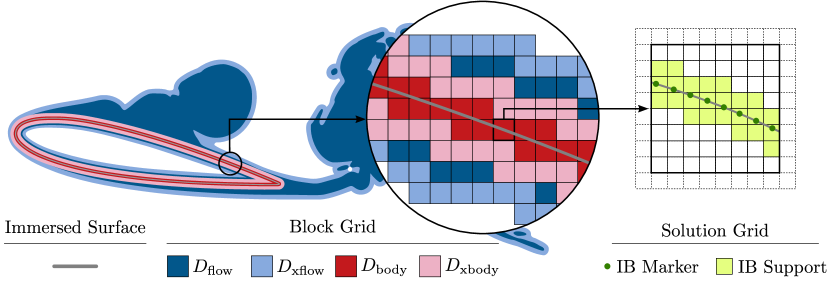
Figure 1: Depiction of a 2D finite computational grid, solution grid, comprised of blocks arranged on a Cartesian grid, block grid. Distant view of nested sub-domains $D_{\text{flow}}\subset D_{\text{xflow}}$ and $D_{\text{body}}\subset D_{\text{xbody}}$, where $D_{\text{body}}\subseteq D_{\text{flow}}$ and $D_{\text{xbody}}\subseteq D_{\text{xbody}}$ (left). Zoomed-in view illustrating the union of blocks used to define the domain (middle). Magnified view of the finite staggered Cartesian grid and IB markers associated with a single block (right). Dashed cells surrounding the interior cells of the isolated block correspond to ghost cells used to facilitate the parallel implementation.

We consider partitioning the unbounded solution grid into blocks arranged on a Cartesian block grid. Approximate values for each term of the IF-HERK and the velocity refresh algorithms are computed by limiting the source (domain) and target (co-domain) regions of discrete operators to the sub-domains depicted in Figure 1. These sub-domains are defined as follows:

• Flow domain $D_{\text{flow}}$: union of blocks containing non-negligible source terms for any discrete Poisson problem solved in the present formulation, i.e. Eq. (21a)–(21c) and velocity refresh. Flow quantities on $D_{\text{flow}}$ are taken to be accurate approximations of the corresponding flow quantities that would have been obtained by numerically operating on the entire unbounded domain.

• Expanded flow domain $D_{\text{xflow}}$: union of blocks that are at most $N_{\text{buf}}^{\text{flow}}$ blocks in any direction from any block in $D_{\text{flow}}$. The value of $N_{\text{buf}}^{\text{flow}}$ is determined using the procedure discussed in [26] so that the error in $D_{\text{flow}}$ remains below a prescribed threshold for the time-steps between velocity refreshes.

• Body blocks $D_{\text{body}}$: union of blocks containing grid cells that are at most one grid cell away from the support of any discrete delta function during a single time-step. This implies, for example, that all non-zero values of $\mathsf{G}^{\dagger}[\mathscr{I}^{\dagger}(t)]$ are contained within $D_{\text{body}}$.

• Expanded body domain $D_{\text{xbody}}$: union of blocks that are at most $N_{\text{buf}}^{\text{body}}\leq N_{\text{buf}}^{\text{flow}}$ blocks in any direction from any block in $D_{\text{body}}$. We limit our attention to the case of $N_{\text{buf}}^{\text{body}}=N_{\text{buf}}^{\text{flow}}=N_{\text{buf}}$, and note that the subsequent discussions readily extend to the general case of $N_{\text{buf}}^{\text{body}}\neq N_{\text{buf}}^{\text{flow}}$.

Unlike domains $D_{\text{flow}}$ and $D_{\text{xflow}}$ which are recomputed only when the grid adapts [26], domains $D_{\text{body}}$ and $D_{\text{xbody}}$ are recomputed at every time-step during which the immersed surface moves.

Summarized in Table 1 are the source and target regions used in the present formulation to evaluate the action of discrete operators with wide, or potentially wide, stencils (discrete kernels), i.e. $\mathsf{L}_{\mathcal{Q}}^{-1}$, $\mathsf{E}_{\mathcal{Q}}(\alpha)$, and $\mathsf{K}^{-1}_{\mathcal{Q}}(\alpha)$. Similar source and target region considerations are readily deduced for all other operators, but are not discussed here since the operation count and propagation of finite boundary errors associated with these compact-stencil operators are significantly smaller than those of the operators listed in Table 1. Also highlighted by Table 1 are the significant operation count reductions achieved by taking advantage of the flexible source and target regions of LGF-FMM for cases involving immersed surfaces with $N_{L}\ll N_{E}$.

Eq.	(21a)∗	(21b)†	(21c)†	(21d)	(22)†	(22)†	(23)
Operator	$\mathsf{L}_{\mathcal{C}}^{-1}$	$\mathsf{H}^{i}_{\mathcal{F}}$	$\mathsf{L}_{\mathcal{C}}^{-1}$	$\mathsf{H}^{i}_{\mathcal{F}}$	$(\mathsf{K}^{i}_{\mathcal{F}})^{-1}$	$\mathsf{H}^{i}_{\mathcal{F}}$	$\mathsf{L}_{\mathcal{F}}^{-1}$
Source	$D_{\text{flow}}$	$D_{\text{xbody}}$	$D_{\text{body}}$	$D_{\text{xflow}}$	$D_{\text{body}}$	$D_{\text{body}}$	$D_{\text{flow}}$
Target	$D_{\text{xflow}}$	$D_{\text{body}}$	$D_{\text{xflow}}$	$D_{\text{xflow}}$	$D_{\text{body}}$	$D_{\text{body}}$	$D_{\text{xflow}}$
Op. Count	$M^{\mathsf{L}}_{\text{f}\rightarrow\text{xf}}$	$3M^{\mathsf{E}}_{\text{xb}\rightarrow\text{b}}$	$M^{\mathsf{L}}_{\text{b}\rightarrow\text{xf}}$	$3M^{\mathsf{E}}_{\text{xf}\rightarrow\text{xf}}$	$M^{\mathsf{K}}_{\text{b}\rightarrow\text{b}}$	$3M^{\mathsf{E}}_{\text{b}\rightarrow\text{b}}$	$3M^{\mathsf{L}}_{\text{f}\rightarrow\text{xf}}$
Op. Scaling	$\mathcal{O}(N_{E})$	$\mathcal{O}(N_{L})$	$\mathcal{O}(N_{E})$	$\mathcal{O}(N_{E})$	$\mathcal{O}(N_{L})$	$\mathcal{O}(N_{L})$	$\mathcal{O}(N_{E})$

Table 1: Source and target regions used to approximate the action of non-compact discrete operators. The number of operations required to compute the action of each operator is denoted in the second to last row; operation counts for vector operations are approximated as three corresponding scalar operations. Superscript $*$ indicates equations originally given in the form $\mathsf{L}\mathsf{x}=\mathsf{y}$ that are written here as $\mathsf{y}=\mathsf{L}^{-1}\mathsf{x}$. Superscript $\dagger$ indicate equations that are not computed for cases without immersed surfaces.

Temporal variations in the non-negligible support regions of discrete operators are facilitated by adding and removing blocks to $D_{\text{flow}}$ and $D_{\text{body}}$ ($D_{\text{xflow}}$ and $D_{\text{xbody}}$ are updated accordingly). At the end of every time-step, flow quantities on a region that is a few grid cells greater than $D_{\text{flow}}$ are used to compute the block-wise weight function $W_{\text{flow}}$ for each block in $D_{\text{xflow}}$, which in turn is used to define $D_{\text{flow}}$ of the next time-step,

$$D^{k+1}_{\text{flow}}=\left\{B:[W_{\text{flow}}(B^{\prime})]>\epsilon_{\text{supp}},\,\,B^{\prime}\in D^{k}_{\text{xflow}}\right\}.$$ (24)

Here, we use the block-wise weight function proposed in [26],

$$W_{\text{flow}}(B)=W(\text{pos}(B))\max_{B\in D_{\text{xflow}}}\left({\mu(B)}/{\mu_{\text{global}}},\,{\nu(B)}/{\nu_{\text{global}}}\right),$$ (25)

where $W(\text{pos}(B))$ is a function of the position of block $B$,

$$\mu(B)=\ \max_{\mathbf{m}\in\text{{ind}}(B)}|\mathsf{w}(\mathbf{n})|,\quad \mu_{\text{global}}=\max_{B\in D_{\text{xflow}}}\mu(B),$$ (26a)

$$\nu(B)=\ \max_{\mathbf{m}\in\text{{ind}}(B)}|\mathsf{h}(\mathbf{n})|,\quad \nu_{\text{global}}=\max_{B\in D_{\text{xflow}}}\nu(B).$$ (26b)

Solution grid variables $\mathsf{w}=\mathsf{C}\mathsf{u}$ and $\mathsf{h}=\overline{\mathsf{D}}\tilde{\mathsf{N}}(\mathsf{u},t)$ correspond to the discrete vorticity and divergence of the Lamb vector.

For the case of $W(\mathbf{r})=1$, Eq. 25 approximates the maximum normalized residual of the discrete Poisson problems Eq. (21a) and (23) resulting from excluding source terms outside of $D_{\text{flow}}$ [26]. Accurate solutions to the laminar-to-turbulence transition of thin vortex rings at Reynolds numbers up to $\numprint{7500}$ resulting in small solution grids near the ring core are reported in [26] using $W(\mathbf{r})=1$. In contrast, small solution grids are not expected to result from flows around immersed surfaces computed with $W(\mathbf{r})=1$ since vorticity is constantly generated at the surface and convected downstream. In practice, we are often interested in accurately reproducing the flow physics in the vicinity of the immersed surface, and are willing to reduce computational costs by neglecting flow features in far-downstream wake regions that do not significantly affect the near-surface flow. Point-wise estimates for the residuals of Eq. (21a) and (23) based on the asymptotic $\mathcal{O}(|\mathbf{n}|^{-1})$ decay of $\mathsf{G}_{\mathsf{L}}$ [28] indicate that errors near the immersed surface resulting from

$$W(\mathbf{r})=\frac{1}{\max\left(\eta,\text{dist}(\mathbf{r})\right)},$$ (27)

where $\eta\geq 1$ is a prescribed parameter and $\text{dist}(\mathbf{r})$ is the non-dimensionalized distance from $\Gamma(t)$, are comparable in magnitude to those resulting from using $W(\mathbf{r})=1$. Unless otherwise stated, subsequent discussions and numerical experiments take $W_{\text{flow}}$ to be given by Eq. (25) and (27).

4.2 Algorithm summary

In this section we summarize the present IB-LGF method for incompressible flows on unbounded staggered Cartesian grids. The sequence of steps performed in the IB-LGF algorithm for an $s$-stage IF-HERK scheme is outlined as follows:

1. Pre-processing [Sec. 3.2]: (rigid surface only, optional) for each unique force Schur complement operator $\hat{\mathfrak{C}}\in\left\{\mathfrak{C}^{i},\forall\,i=[1,s]\right\}$, build its dense SPD matrix representation $\mathbf{C}$ by applying the operator to each standard basis vector, compute the Cholesky decomposition of $\mathbf{C}$ and invert the Cholesky factor $\mathbf{L}$ using ScaLAPACK, and store $\mathbf{W}=\mathbf{L}^{-1}$.

2. Time integration: for the $k$-th time-step:

   1. Grid body update [Sec. 4.1]: use the prescribed motion of $\Gamma(t)$ and the support region of discrete delta functions to compute $D_{\text{body}}$ and $D_{\text{xbody}}$ for $t\in[t_{k},t_{k+1}]$.

   2. Grid flow update [Sec. 4.1]: use $D_{\text{body}}\subseteq D_{\text{flow}}$, weight function $W_{\text{flow}}$, threshold values $\epsilon_{\text{supp}}$, and $\mathsf{w}_{k}\leftarrow\mathsf{C}\mathsf{u}_{k}$ and $\mathsf{h}_{k}\leftarrow\overline{\mathsf{D}}\tilde{\mathsf{N}}(\mathsf{u}_{k},t_{k})$ to construct new $D_{\text{flow}}$. If necessary, update old $D_{\text{flow}}$ and $D_{\text{xflow}}$ by adding or removing blocks. Copy $\mathsf{w}_{k}$ from the old to the new solution grid and zero values on $D_{\text{buffer}}$.

   3. Velocity refresh [Sec. 4.1]: if either $D_{\text{body}}$ has been updated or the number of time-steps since last refresh exceeds $Q_{\text{max}}$, compute $\mathsf{u}_{k}$ from $\mathsf{w}_{k}$ using Eq. (23).

   4. IF-HERK [Sec. 2.3]: compute $\mathsf{u}_{k+1}$, ${t}_{k+1}$, $\mathsf{q}_{k+1}$, and $\mathfrak{f}_{k+1}$ using $\text{xIF-HERK}(\mathsf{u}_{k},t_{k})$, where xIF-HERK is the version of the IF-HERK algorithm that restricts the source and target regions of discrete operators to finite sub-regions of the solution grid, e.g. operations defined in Table 1. Linear systems arising at each RK stage are solved using the nested projection technique Eq. (21) with an appropriate body forces solver (Section 3.2).

An operation count estimate for a single time-step based on the action of all non-compact operators, i.e. operators listed in Table (1) and $\mathfrak{C}^{-1}$, is given by $M=M_{\text{flow}}+M_{\text{ib}}$, where $M_{\text{flow}}$ is the number of operations used to solve the flow without immersed surfaces [26],

$$M_{\text{flow}}=sM^{\mathsf{L}}_{\text{f}\rightarrow\text{xf}}+3C(s)M^{\mathsf{E}}_{\text{xf}\rightarrow\text{xf}}+\lceil 3M^{\mathsf{L}}_{\text{f}\rightarrow\text{xf}}\rfloor,$$ (28)

$M_{\text{ib}}$ is the number of operations required to compute the additional IB terms,

$$M_{\text{ib}}=sM^{\mathsf{L}}_{\text{b}\rightarrow\text{xf}}+sM^{\mathfrak{C}}_{\text{f}\rightarrow\text{f}}+3sM^{\mathsf{E}}_{\text{xb}\rightarrow\text{b}},$$ (29)

and $M^{\mathfrak{C}}$ is the number of operations used to solve for the body forces. For a general $s$-stage HERK scheme with second-order accurate constraint variables $C(s)$ is equal to $s+\left((s-1)s\right)/2-1$ [26]. The last term in Eq. (28) is associated with the vector Poisson solve (roughly equal to three scalar Poisson solves) required by the velocity refresh procedure, which is not necessarily performed at every time-step as indicated by the notation $\lceil\,\cdot\,\rfloor$. All terms in Eq. (28) and (29), except for $M^{\mathfrak{C}}_{\text{f}\rightarrow\text{f}}$ and $M^{\mathsf{E}}_{\text{xb}\rightarrow\text{b}}$, scale as $\mathcal{O}(N_{E})$. The term $M^{\mathsf{E}}_{\text{xb}\rightarrow\text{b}}$ scales as $\mathcal{O}(N_{L})$ and, for typical flows, is negligible compared to any of the $M^{\mathsf{L}}_{x}$ terms. Estimates and scaling for $M^{\mathfrak{C}}_{\text{f}\rightarrow\text{f}}$ are discussed in Section 3.2, but we note here that computation time spent solving for body forces is less than 3% of the total run time for all test cases included in Section 5.

The present MPI-based parallel implementation partitions and distributes the support of the discrete delta functions according to the block-wise partition and distribution of the solution grid. Values for all IB markers are taken to be known by all processors, which is accomplished by having values broadcast before and aggregated after the application of $\mathscr{I}^{\dagger}$ and $\mathscr{I}$, respectively. Details regarding the parallel implementation of the flow solver, i.e. the IB-LGF method without an immersed surface, are discussed in [26, 28]. Load balancing is performed every time $D_{\text{flow}}$ or $D_{\text{xflow}}$ are updated. This operation consists of optimizing the most computationally expensive operations, i.e. Eq. (21a) and (23), following the procedure described in [28] with the additional requirement of having all blocks belonging to $D_{\text{body}}$ be distributed as equally as possible across all processors. Each RK stage of the representative problems of Section 5 is evaluated at a typical computation rate (normalized by the total number of MPI processes) of approximately 80 micro-seconds per active grid cell or, equivalently, 20 micro-seconds per active flow variable (3 velocity components and 1 pressure per grid cell).

Lastly, we clarify that the LGF-FMM [28] and the LGF flow solver [26] are direct solvers that compute solutions to prescribed tolerances based on a set of parameters. Aside from convergence criteria required for the case of iterative boundary force solutions, the IB-LGF method does not depend on any additional parameters beyond those of the LGF flow solver [26]. Furthermore, having limited our attention to cases with $D_{\text{body}}\subseteq D_{\text{flow}}$, $D_{\text{xbody}}\subseteq D_{\text{xflow}}$, and $N^{\text{body}}_{\text{buf}}=N^{\text{flow}}_{\text{buf}}$ ensures that the procedures of LGF flow solver used to determine appropriate values for all parameters based on single threshold $\epsilon^{*}$ extend to the IB-LGF method. Subsequent discussions take $\epsilon^{*}$ to be equal to the grid adaptivity parameter $\epsilon_{\text{supp}}$.

5 Verification examples

Numerical experiments on flows around infinitely thin rectangular flat plates and spherical shells are used to verify the IB-LGF method. Rectangular flat plates are generated by a set of IB markers arranged in a 2D uniform Cartesian grid with a prescribed aspect-ratio AR and angle-of-attack $\alpha$. Spherical shells, subsequently referred to as spheres, are generated by placing IB markers at the centroids of the faces of an icosphere. Icospheres are triangulated surfaces constructed by recursively subdividing the faces and radially projecting newly created vertices onto the unit sphere of an initial icosahedron [48]. The ratio of the minimum to maximum distances between any two IB markers tends to approximately 0.28 after a large number of subdivisions.

For all test cases, the minimum spacing between any two IB markers, ${\Delta s}^{*}$, is taken to be approximately equal to the grid spacing ($1.0<{\Delta s}^{*}/\Delta x<1.1$), and the smoothed version [49] of the 3-pt $\delta_{h}$ [24] is used to construct $\mathscr{I}$. Boundary forces are computed using the parameter-free Cholesky pre-processing technique discussed in Section 3.2. Unless otherwise stated, the adaptivity threshold parameter $\epsilon^{*}$ is taken to be $5\times 10^{-4}$, a choice that will be justified in Section 5.3. All test cases, except those for the temporal refinement studies, are performed using the HERK coefficients of Scheme A included in B and are subject to the CFL condition $|\mathbf{u}|\Delta t/\Delta x<1$. The time-step size is specified so that the CFL based on the maximum point-wise velocity remains below $0.5$ and $0.9$ for flows at $\text{Re}\leq\numprint{500}$ and $\text{Re}=\numprint{3700}$, respectively, except for the first few time-steps of impulsively started flows during which the CFL is allowed to be approximately equal to unity. We clarify that the average CFL for spheres at $\text{Re}=\numprint{3700}$ is approximately $0.6$, which is significantly lower than the large-time maximum of $0.9$.

5.1 Discretization error

The convergence rates of the discretization technique is examined through spatial and temporal refinement studies of flows around spheres of radius $D$ with a prescribed velocity $\mathbf{U}(t)=\left(U_{x}(t),0,0\right)$,

$$U_{x}(t)=\left\{\begin{array}[]{cl}4\beta U\displaystyle\int_{0}^{t}e^{\frac{-1}{1-\left(4t^{\prime}-1\right)^{2}}}\,dt^{\prime}&\text{for}\,\,0\leq\frac{tU}{D}\leq\frac{1}{2}\\ U&\text{for}\,\,\frac{1}{2}<\frac{tU}{D}\end{array}\right.,$$ (30)

where $\beta\simeq 2.25228$ is taken so that $U_{x}(t)$ is infinitely differentiable for all $t$ (assuming $U_{x}(t)=0$ for $t<0$). The instantaneous Reynolds number $\text{Re}=U_{x}(t)D/\nu$ levels to a constant equal to $100$ for $t>\frac{1}{2}D/U_{\infty}$. All numerical experiments discussed in this section are performed using $\epsilon^{*}=10^{-8}$.

The spatial convergence study is performed using a total of seven test cases, S.I–S.VII, corresponding to spheres generated by $20\times 4^{i-1}$ for $i=1,2,\dots,8$ IB markers. The time-step size, $\Delta t$, is held fixed across all test cases, and chosen so that the maximum CFL for S.VII is less than $0.25$. Estimates for the errors obtained by taking S.VII to be the reference, or true, solution are reported in Figure 2. As expected from analysis [50, 51] and numerical experiments [9, 10, 11] of similar IB methods, the velocity $\mathbf{u}\approx\mathsf{u}$ is verified to be first-order accurate in the $L_{\infty}$ norm. Less intuitive is the fact that the pressure $p\approx\mathsf{p}$ and the net body force $\mathbf{F}\approx\sum_{i}\mathfrak{f}_{i}$ also exhibit first-order convergence rates under the $L_{\infty}$ norm.

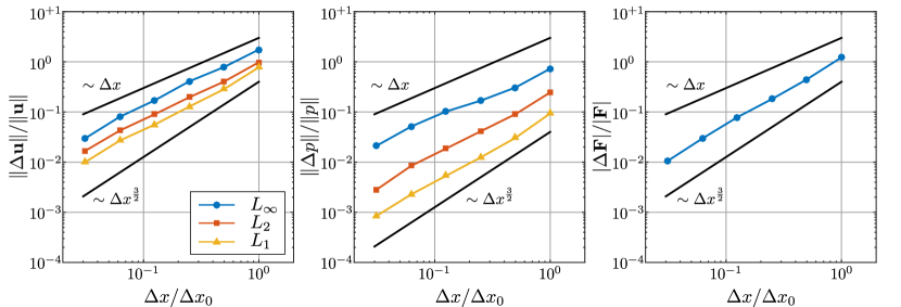
Figure 2: Differences in the velocity (left), pressure (middle), and net body force (right) for different values of $\Delta x$ while holding $\Delta t$ fixed. The value of $\Delta x_{0}$ is equal to $\Delta x$ of coarsest test case (S.I).

It is well-known that the spatial smoothing inherent to the regularized delta function treatment of the immersed surfaces is unable to correctly capture the discontinuous pressure across interfaces. The spatial regularization resulting from $\delta_{h}$ has been shown to lead to $\mathcal{O}(1)$ errors in the pressure near the immersed surface [50, 52], which in turn prevents the $L_{\infty}$ convergence of the discrete pressure to the actual, continuum pressure. The first-order $L_{\infty}$ convergence rate of the pressure shown in Figure 2 is a consequence of taking the reference solution to be that of S.VII as opposed to the actual solution to Eq. (1). Convergence rates equal or greater to first-order follow from the fact that the continuum pressure across surfaces regularized by $\delta_{h}(\mathbf{x})$ is continuous and differentiable (provided a sufficiently smooth $\delta_{h}$) [53]. However, for the present refinement study the convergence rate is at most first order since the regularization length-scale $h$ is taken to be equal to $\Delta x$ of the reference (finest) solution and, as a result, will change as progressively finer test cases are considered.

Next, we consider the slightly greater than first-order convergence rate of the body forces. Surface stresses obtained from most IB methods are known to exhibit less than first-order point-wise convergence rates [49, 11, 37] and can even grow as the immersed surface is refined [37]. Yet, it is also known that the low-order moments for the surface stresses, such as the net force on the immersed body, are physically accurate. This is verified by the right plot of Figure 2, which shows that the net body force, $\mathbf{F}$, convergence at a rate that is slightly greater than first-order. Approximate first-order convergence rates for the net force on rigid surfaces also have been demonstrated for other IB-DLM methods [11, 37].

Lastly, we report the $L_{2}$ condition number, $\kappa$, of the force Schur complement of the last RK stage, $\mathfrak{C}^{s}$, for each test case in Table 2. As points of comparison, Table 2 also includes values for $\kappa$ resulting from using values $\Delta s^{*}/\Delta x$ that are smaller ($1.00$ and $0.95$) than those used for S.I–S.VII ($1.05$). Table 2 verifies the intuitive fact, based on the finite spatial resolution of the fluid solver, that the matrix corresponding to $\mathfrak{C}^{s}$ rapidly becomes ill-conditioned for values $\Delta s/\Delta x$ below certain threshold, which is approximately unity for the present test cases. The heuristic constraint of requiring $\Delta s^{*}/\Delta x\geq 1$ is not universal across IB-DLM methods; [10] states that $\Delta s/\Delta x\approx 1$ results in “reasonable” condition numbers for $\mathfrak{C}$-like matrices computed using the 3-pt $\delta_{h}$ of [24], and [11] numerically demonstrates that $\Delta s/\Delta x\approx 2$ results in condition numbers for $\mathfrak{C}$-like matrices computed using the 6-pt $\delta_{h}$ of [54] comparable to those listed in Table 2 for the case of steady Stokes flow around a sphere. We clarify that, in the continuum limit, the boundary integral operator associated with $\mathfrak{C}$ has a zero-eigenvalue mode corresponding to the uniform compression of the sphere. Typically, we expect that the small geometric irregularities, strict symmetry-breaking, and slight porosity of numerical immersed surfaces generated using standard discrete delta functions and well-spaced IB-markers, i.e. $\Delta s/\Delta x\approx 1$, to result in non-singular discrete $\mathfrak{C}$ operators, even if the continuous version of $\mathfrak{C}$ is singular. Small-eigenvalue discrete modes associated with zero-eigenvalue continuous modes that do not satisfy the continuous divergence-free constraint are expected to be only a small part of the solution of $\mathfrak{C}\mathfrak{f}=\mathfrak{r}$, i.e. the dot product of these modes with $\mathfrak{r}$ is small, since $\mathfrak{r}$ is interpolated from a discrete divergence-free field. Additional discussions and numerical examples regarding the null-space, or lack thereof, and conditioning of $\mathfrak{C}$-like operators arising in other IB-DLM discretizations are provided in [11, 37]. Here, the results of Table 2 are used to verify the well-posedness of Eq. (8) as a (solvable) DAE system of index 2 and to motivate the nominal value of $\Delta s^{*}\approx 1.05\Delta x$ used in subsequent numerical experiments.

No. IB markers	$\numprint{20}$	$\numprint{80}$	$\numprint{320}$	$\numprint{1280}$	$\numprint{5120}$	$\numprint{20480}$	$\numprint{81920}$
$\Delta s^{*}/\Delta x\simeq 1.05$	0.19	0.20	0.18	0.17	0.19	0.44	1.31
$\Delta s^{*}/\Delta x\simeq 1.00$	0.19	0.52	0.36	0.42	1.61	1.41	–
$\Delta s^{*}/\Delta x\simeq 0.90$	2.06	3.13	1.72	2.69	8.51	27.94	–

Table 2: $L_{2}$ condition number of $\mathfrak{C}^{s}$ for different ratios of $\Delta s^{*}/\Delta x$. Values of $\Delta s^{*}/\Delta x\simeq 1.05$ are used in the numerical experiments S.I–S.VII.

We now turn our attention to the temporal discretization error. The temporal convergence studies are performed for each of the four IF-HERK schemes included in B, Scheme A – D, for a sphere generated by 1280 IB markers. A total of nine test cases, T.I – T.IX, of varying time-step size, $\Delta t/\Delta t_{0}=2^{-i+1}$ for $i=1,2,\dots,9$, are considered for each scheme. Here, $\Delta t_{0}$ is chosen such that the maximum CFL of test case T.I is less than $0.5$. Error estimates for each test case are obtained by taking T.IX of the corresponding IF-HERK scheme to be the reference solution. The $L_{\infty}$ norm of the errors, depicted in Figure 3, verifies that the computed convergence rates of each IF-HERK scheme with respect to $\Delta t$ is equal to the expected order of accuracy based on the HERK order conditions discussed in Section 2.3 and B.

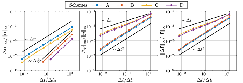
Figure 3: Differences in the velocity (left), pressure (middle), and net body force (right) for different values of $\Delta t$ while holding $\Delta x$ fixed. The value of $\Delta t_{0}$ is equal to $\Delta t$ of coarsest test case (T.I). Entries for the velocity error for Scheme B and D that are below $10^{-8}$ are excluded from the left plot since the error for these cases saturates between $10^{-9}$ and $10^{-8}$ due to prescribed adaptivity threshold $\epsilon^{*}=10^{-8}$.

We emphasize that the refinement studies of this section have only verified that numerical solutions converge at the expected rate under $\Delta x$ and $\Delta t$ refinements. The tests cases discussed in the following sections will demonstrate that the computed solutions are in fact accurate physical approximation to Eq. (1).

5.2 Flow around low-aspect-ratio rectangular plates

The physical fidelity of the IB-LGF method is verified in this section by comparing solutions for impulsively-started rectangular flat plates of chord-length $c$ and area $A$ to previously published results. We begin by considering the experimentally-validated test cases [55] of flows around plates of $AR=2$ at $\text{Re}=100$ and $0^{\circ}\leq\alpha\leq 90^{\circ}$. Here, test cases are performed taking $\Delta x=0.020c$, which is comparable to the near-surface grid spacing of $0.025c$ used to compute these flows by other IB methods [55, 23]. Previous refinement studies and comparisons with experimental data [55] indicate that the flow is sufficiently well-resolved using the present value of $\Delta x$.

The left plot of Figure 4 demonstrates that the computed drag and lift coefficients, $C_{\text{D}}=-F_{x}/(\frac{1}{2}\rho U^{2}A)$ and $C_{\text{L}}=F_{y}/(\frac{1}{2}\rho U^{2}A)$, at $tU/c=13$ are in good agreement with previously reported values [55, 23]. The force coefficients from the three methods are nearly indistinguishable for $0^{\circ}\leq\alpha\leq 50^{\circ}$ and by less than 5% for $60^{\circ}\leq\alpha\leq 90^{\circ}$. The large-time ($50\leq tU/c\leq 75$) behavior of the mean and fluctuating components of $C_{\text{D}}$ and $C_{\text{L}}$ are summarized in the right plot of Figure 4. This plot demonstrates that for $60^{\circ}\leq\alpha<90^{\circ}$ the flow is unsteady and that the large-time mean forces are significantly different from the instantaneous forces at $tU/c=13$. For $\alpha=60^{\circ}$ and $\alpha=70^{\circ}$ the flow is periodic with Strouhal numbers $\text{St}=F_{y}c\sin\alpha/U$ equal to $0.13$ and $0.11$, respectively. In contrast, for $\alpha=80^{\circ}$ and $\alpha=90^{\circ}$ the flow is a aperiodic (at least during $50\leq tU/c\leq 75$) since the force coefficients neither have a constant mean value nor a clear dominant frequency. We suspect that the sensitivity of instantaneous measurements of unsteady flows to small perturbations is responsible for the larger differences across the three numerical investigations presently considered for test cases with $60^{\circ}\leq\alpha\leq 90^{\circ}$ when compared to the same differences for test cases with $0^{\circ}\leq\alpha\leq 50^{\circ}$.

Figure 4: Drag and lift coefficients for rectangular flat plates of $\text{AR}=2$ at $\text{Re}=100$ and different values of $\alpha$. Instantaneous values at $tU/c=13$ (left). Range (shaded regions) and mean value (solid circles) of force coefficients during $50\leq tU/c\leq 75$ (right).

Next, we consider impulsively started plates of different ARs at $\alpha=30^{\circ}$ and $\text{Re}=300$. Previous numerical experiments on these flows [55, 23, 56] have used grid spacings of approximately $0.025c$ in the immediate vicinity of the plate (same as for the previously referenced $\text{Re}=100$ test cases). Here, each flow is computed using (A) $\Delta x=0.025c$ and (B) $\Delta x=0.015c$.

Vortical structures in the wake of plates of $\text{AR}=1,\,2,\,\text{and}\,\,4$ are illustrated as iso-surfaces of constant vorticity strength in Figure 5. The depicted structures are in good visual agreement with the structures reported in previous numerical experiments for $\text{AR}=1,2,4$ [55] and $\text{AR}=4$ [23, 56]. Also shown in Figure 5 are snapshots of cross-sectional cuts of the finite computational domains resulting from the block-wise adaptive computational grid algorithm. As expected from the adaptivity criteria discussed in Section 4.1, strong vortical regions near the immersed surface are efficiently tracked by adding and removing computational blocks. For the test case of $\text{AR}=4$, the stream-wise length of the union of blocks is approximately $[-1c,9c]$ (about the leading edge), which can be compared to the stream-wise length $[-4c,6.1c]$ of the finite domain (with approximate boundary conditions) used in [55, 23].

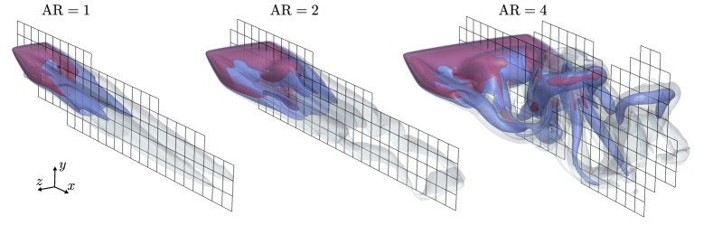
Figure 5: Vortices in the wakes of rectangular flat plates of different ARs at $\alpha=30^{\circ}$ and $\text{Re}=300$. Shown above are iso-surfaces of $|\boldsymbol{\omega}|c/U=2,4,8$ at $tU/c\simeq 46.2$ computed using $\Delta x=0.015c$. The union of boxes shown on the $x-y$ plane centered about the plate center depict the cross-sectional cut of the block-wise adaptive computational domain. Depicted blocks have been coarsened by a factor of two in each direction for visualization purposes.

The large-time ($50\leq tU/c\leq 80$) temporal statistics for the force coefficients of the plates depicted in Figure 5 are included in Table 3. Strouhal numbers of $0.12$ for $\text{AR}=4$ obtained for (A) and (B) are also reported in [55, 23]. For all ARs, differences in mean force coefficients between (B) and [55, 23, 56] are less than 12%. The effect of the grid resolution on the accuracy of the solution can be approximated by comparing the results of the low-resolution test cases (A) with the results of the high-resolution test cases (B). The values of Table 3 indicate that the differences in mean force coefficients between (A) and (B) are less than 4% for all ARs. Since the grid resolutions of (A) and [55, 23, 56] are approximately the same, we suspect that modeling errors resulting from the small computational domains and approximate boundary conditions used in [55, 23, 56] account for most of the differences in the mean force values.

	$\text{AR}=1$		$\text{AR}=2$		$\text{AR}=4$
	$C_{\text{D}}$	$C_{\text{L}}$	$\overline{C_{\text{D}}}$	$\overline{C_{\text{L}}}$	$\overline{C_{\text{D}}}$	$\Delta C_{\text{D}}$	$\overline{C_{\text{L}}}$	$\Delta C_{\text{L}}$	St
Present (A)	0.543	0.627	0.504	0.571	0.620	0.018	0.791	0.074	0.118
Present (B)	0.526	0.644	0.488	0.587	0.593	0.016	0.798	0.053	0.124
TC09 [55]	0.56	0.60	0.53	0.57	0.66	–	0.80	–	0.12
WZ11 [23]	–	–	–	–	–	–	–	–	0.12
WZ13 [56]	–	–	–	–	–	–	0.79	–	–

Table 3: Drag and lift coefficients, and Strouhal numbers for rectangular flat plates of different ARs at $\alpha=30^{\circ}$ and $\text{Re}=300$. Present (A) and (B) correspond to test cases computed using $\Delta x/c=2.5\times 10^{-2}$ and $\Delta x/c=1.5\times 10^{-2}$, respectively. Results from TC09 – Taira and Colonius [55], WZ11 – Wang and Zhang [23], and WZ13 – Wang et al. [56] are also provided.

5.3 Flow around spheres

In this section we further verify the IB-LGF method by computing flows around impulsively started spheres. A small perturbation $(0,\hat{u}(t),0)$ is introduced to the nominal velocity of the sphere $(U,0,0)$ in order to break axial symmetry. We take $\hat{u}(t)$ to be non-zero for $1<tU/D<\frac{4}{3}$ with values equal to the bump function $\frac{1}{10}Ue^{1-1/(1-\tau^{2})}$ with $\tau=8t-9$. Net body forces are reported as non-dimensional force coefficients $C_{q}=F_{q}/(\frac{1}{2}\rho U^{2}\pi(\frac{D}{2})^{2})$ for $q\in\{x,y,z\}$, and correspond to the drag ($C_{\text{D}}=C_{x}$), lateral ($C_{\text{L}}=C_{y}$), and side ($C_{\text{S}}=C_{z}$) coefficients.

First, we demonstrate that the grid adaptivity criteria and the nominal threshold value $\epsilon^{*}=5\times 10^{-4}$ accurately capture the unbounded domain flow by only tracking the solution on a small, finite region near the surface and immediate wake of a sphere at $\text{Re}=300$. Periodic flows exhibiting planar symmetry are limited to a narrow range of Reynolds numbers that has been numerically estimated to be $280<\text{Re}<375$ [57, 58]. The temporal periodicity and spatial symmetry about the $x$-$y$ plane of the flow [57, 59, 60] makes this test case a challenging problem that still permits meaningful force coefficient comparisons.

The time histories for $C_{\text{D}}$ and $C_{\text{L}}$, and snapshots of the vorticity field for spheres generated by $\numprint{20480}$ IB markers ($\Delta x\simeq 9.33\times 10^{-3}$) computed with values of $\epsilon^{*}=5\times 10^{-i}$ for $i=2,\,3,\,4,\,\text{and}\,\,5$ are shown in Figure 6. The maximum value of $|C_{\text{S}}|$ for $0\leq tU/D\leq 90$ is less than $2\times 10^{-2}$, $1\times 10^{-2}$, $5\times 10^{-3}$, and $2\times 10^{-3}$, respectively, for the present test cases sorted in decreasing order of $\epsilon^{*}$, which in turn confirm the expect planar symmetry of the flow. Periodic oscillations in the time history of force coefficients are clearly observed for $\epsilon^{*}\leq 5\times 10^{-4}$, but not for $\epsilon^{*}\geq 5\times 10^{-3}$. The apparent stabilization of the flow for $\epsilon^{*}\geq 5\times 10^{-3}$ is expected from the fact that the finite computational domains of these test cases do not support a complete wavelength of the wake instability. In contrast, the computational domain of $\epsilon^{*}=5\times 10^{-4}$ supports at least one full wavelength of the instability and is able to accurately reproduce the large-time mean and oscillatory components of $C_{\text{D}}$ and $C_{\text{L}}$ obtained by the most conservative test case, i.e. $\epsilon^{*}=5\times 10^{-5}$.

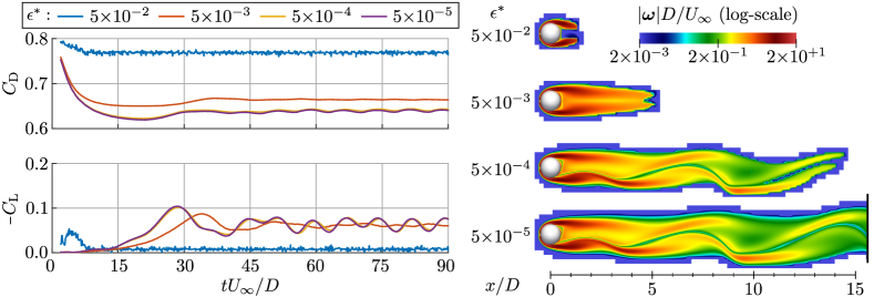
Figure 6: Flow around a sphere at $\text{Re}=300$ computed using different adaptive threshold, $\epsilon^{*}$, values. Time history of drag and lateral force coefficients (left). Side-view of finite computational domains at $tU/D=80.3$ (right). For each case, the finite computational domain corresponds to the non-white region near the body and its wake. For the case of $\epsilon^{*}=5\times 10^{-5}$ the finite computational domain continues for an additional $15D$ beyond solid black line.

Quantitative estimates for the errors resulting from non-zero values of $\epsilon^{*}$ are computed here as the differences in the force coefficient $C$ between two test cases:

$$\varepsilon^{I}(C)=\textstyle\max_{t\in T_{A}}{\left|C(t)-C^{\prime}(t)\right|},\,\,\varepsilon^{II}_{\text{{ext}}}(C)=\left|\text{{ext}}_{t\in T_{B}}{C(t)}-\text{{ext}}_{t\in T_{B}}{C^{\prime}(t)}\right|,$$ (31)

where $T_{A}U/D=[2,30]$, $T_{B}U/D=[75,90]$, and ext is either the minimum ($\min$) or maximum ($\max$) extremum. Error estimates obtained by taking the force coefficients of $\epsilon^{*}=5\times 10^{-5}$ to be the reference values are provided in Table 4. As expected, the error associated with neglecting values outside $D_{\text{flow}}$ based on the criteria of Section 4.1 is approximately proportional to $\epsilon^{*}$. The results of Table 4 indicate that, in the absence of discretization errors, the forces computed using the nominal threshold, $\epsilon^{*}=5\times 10^{-4}$, are accurate up to 0.6% of the actual physical forces.

$\epsilon^{*}$	$\varepsilon^{I}(C_{\text{D}})$	$\varepsilon^{II}_{\text{min}}(C_{\text{D}})$	$\varepsilon^{II}_{\text{max}}(C_{\text{D}})$	$\varepsilon^{I}(C_{\text{L}})$	$\varepsilon^{II}_{\text{min}}(C_{\text{L}})$	$\varepsilon^{II}_{\text{max}}(C_{\text{L}})$
$5\times 10^{-2}$	0.1600	0.1117	0.1386	0.1038	0.0470	0.0522
$5\times 10^{-3}$	0.0311	0.0269	0.0235	0.0509	0.0108	0.0116
$5\times 10^{-4}$	0.0030	0.0027	0.0022	0.0041	0.0003	0.0002

Table 4: Estimates for the error resulting from non-zero values of $\epsilon^{*}$ for a sphere at $\text{Re}=300$. Reference values, i.e. $C^{\prime}$ in Eq. (31), are taken from test case with $\epsilon^{*}=5\times 10^{-5}$.

Having verified the error of the adaptive grid, we now turn our attention to confirming the physical fidelity of the IB-LGF method by comparing with previous investigations of flow around spheres. Large-time ($90\leq tU/D\leq 150$) force statistics of spheres computed at $\text{Re}=100,\,200,\,\text{and}\,\,300$ are compared in Table 5. The flow is steady and axi-symmetric at $\text{Re}=100$, and steady and planar $x$-$y$ symmetric at $\text{Re}=250$. At $\text{Re}=250$ and $\text{Re}=300$ the absence of axial symmetry results in a non-zero $C_{\text{L}}$. Values computed using a coarse ($\numprint{5120}$ IB markers and $\Delta x\simeq 1.8\times 10^{-2}$) and a fine ($\numprint{20480}$ IB markers and $\Delta x\simeq 8.8\times 10^{-3}$) grid are shown by Table 5 to be consistent with the range of previously reported values.

	$\text{Re}=100$		$\text{Re}=250$		$\text{Re}=300$
		$C_{\text{D}}$	$C_{\text{D}}$	$C_{\text{L}}$	$\overline{C_{\text{D}}}$	$\Delta C_{\text{D}}$	$\overline{C_{\text{L}}}$	$\Delta C_{\text{L}}$	St
Present (A)		1.084	0.709	0.060	0.665	0.0024	0.067	0.013	0.133
Present (B)		1.086	0.694	0.059	0.656	0.0024	0.065	0.014	0.134
JP99 [57]		1.10	–	0.062	0.656	0.0035	0.069	0.016	0.137
TO00 [59]		–	–	–	0.671	0.0028	–	–	0.136
KK01 [61]		1.087	0.701	0.059	0.657	–	0.067	–	0.134
PW02 [60]		–	–	–	0.683	0.0025	0.061	0.014	0.135
CS03 [62]		–	0.70	0.062	0.655	–	0.065	–	0.136
WZ11 [23]		1.13	–	–	0.68	–	0.071	–	0.135

Table 5: Drag and lift coefficients, and Strouhal numbers for a sphere at different Reynolds numbers. Present (A) and (B) correspond to test cases computed using $\Delta x/D\simeq 1.8\times 10^{-2}$ and $\Delta x/D\simeq 8.8\times 10^{-2}$, respectively. Results from JP99 – Johnson and Patel [57], TO00 – Tomboulides and Orszag [59], KK01 – Kim et al. [61], PW02 – Ploumhans et al. [60], CS03 – Constantinescu and Squires [62], and WZ11 – Wang and Zhang [23] are also provided.

The spread of values shown in Table 5 for spheres at $\text{Re}=300$ indicates that this test case is difficult to compute accurately. The large spread of values for $\Delta C_{\text{L}}$ and $\Delta C_{\text{D}}$ (largest spread based on relative differences) has been attributed to differences in the domain size and boundary conditions of different numerical methods [60]. Consistent with this argument are the small differences in $\Delta C_{\text{L}}$ and $\Delta C_{\text{D}}$ between the present (B) results and those of the unbounded domain vortex method [60].

The numerical experiments on spheres discussed thus far have considered the steady axis-symmetric ($\text{Re}=100$), the steady planar-symmetric ($\text{Re}=250$), and the periodic planar-symmetric ($\text{Re}=300$) flow regimes. Next we verify that the flow is unsteady with no fixed planar symmetry at $\text{Re}=500$ [59, 60]. Figure 7 provides snapshots of stream-wise vorticity iso-surfaces for the aforementioned flow regimes (case of $\text{Re}=100$ is not shown since stream-wise vorticity is of negligible magnitude). The flow at $\text{Re}=500$ is approximately symmetric about the $x$-$y$ plane at early times (similar to the $\text{Re}=300$ test case), but such symmetry is lost at later times as shown in Figure 7 by the axial rotation of the stream-wise vortices.

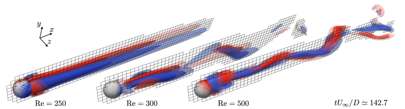
Figure 7: Stream-wise ($x$-direction) vortices in the wake of spheres at different Reynolds numbers depicted as iso-surfaces of constant $\omega_{x}$. Iso-surfaces are for values of $\omega_{x}=\pm 0.20,\,0.10,\,\text{and}\,\,0.05$ at $\text{Re}=250$, and of $\omega_{x}=\pm 1.0,\,0.50,\,\text{and}\,\,0.25$ at $\text{Re}=300\,\,\text{and}\,\,500$. Depicted boxes are described in the caption of Figure 5.

As a final demonstration of the IB-LGF method, we consider the turbulent flow around a sphere at $\text{Re}=\numprint{3700}$. This flow has been characterized in previous numerical [63, 22, 64] and experimental [65] investigations. The flow is computed for $0\leq t^{*}/U\leq 60$ using $\numprint{81920}$ markers and $\Delta x\simeq 4.3\times 10^{-3}$, where $t^{*}$ is used to indicate that flow was initialized from the large-time solution of a sphere at $\text{Re}=\numprint{1000}$. Subsequently reported time-averaged values are computed over the last five large-scale vortex shedding cycles ($\text{St}=0.215$ [64]).

The thin boundary layer on the surface of the sphere is expected to be sufficiently well-resolved since the present value of $(\Delta x)\text{Re}^{\frac{1}{2}}$ (scaling based on the expected $\mathcal{O}(\text{Re}^{-\frac{1}{2}})$ laminar boundary layer thickness [66]) is between the values of $(\Delta x)\text{Re}^{\frac{1}{2}}$ used to compute test cases (A) and (B) at $\text{Re}=300$. As a point of reference, spheres at $\text{Re}=\numprint{3700}$ have been previously computed using a IB/LES method combined with a stretched grid with a near-surface minimum spacings of $9\times 10^{-3}D$ [22] and using a unstructured mesh with a near-surface minimum element side lengths of $1.5\times 10^{-3}D$ [64]. The a posteriori grid analysis of [64] demonstrates that the turbulent flow, with a minimum Kolmogorov length scale of $\eta/D=1.34\times 10^{-2}$ occurring in the $x/D<3$ wake region, is well-resolved by a second-order unstructured mesh with an average element side length of $\overline{h}/D=8\times 10^{-3}$ over the $x/D<3$ wake region. Based on these grid considerations, we assume that the present set of grid parameters are adequate to capture both the thin laminar boundary layer on the surface and the turbulent wake of the flow.

The core of vortical structures in the wake are depicted as iso-surfaces of constant $Q$-value in Figure 8. The $Q$-criterion [67] defines coherent vorticies as connected regions where $Q$, the second invariant of $\nabla\mathbf{u}$, is positive. Positive $Q$-values indicate a local excess of the rotation rate compared to the strain rate. Figure 8 confirms the previously reported [22, 64] pronounced helical-like pattern of large-scale vortical structures in wake. A visual analysis of multiple snapshots verifies that the dominant vorticies forming the helical-like pattern are convected downstream without significant axial rotations and that the pattern is the result of the apparent random azimuthal position of growing shear layer instabilities [22, 64]. We clarify that the strong small-scale vortical filament- and horseshoe-like structures in the downstream wake regions shown in Figure 8 are not readily seen in comparable plots of previous numerical experiments [22, 64], but this is expected from the fact that these previous experiments aggressively coarsen downstream grid regions.

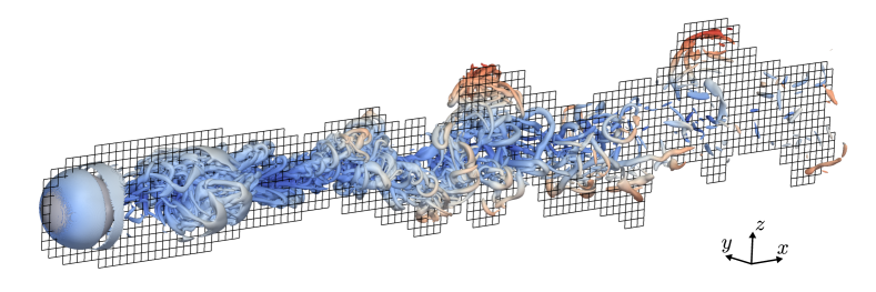
Figure 8: Vortex cores in the wake of a sphere at $\text{Re}=\numprint{3700}$ are illustrated by iso-surfaces of constant $Q$-value. Depicted are iso-surface of $QD^{2}/U^{2}=2$ colored according to the radial distance from the center-line of the sphere in the stream-wise direction. Depicted boxes are described in the caption of Figure 5.

We further characterize the flow by reporting on the large-time mean surface stresses and net body forces. The $i$-th component of the stress vector, $\sigma_{i}=\left[\mathbf{t}\right]_{i}$, at the location of the $q$-th IB marker can be approximated as $\sigma_{i}(\boldsymbol{\xi}_{q})\approx\left[\mathbf{f}_{q}\right]_{i}/A_{q}$, where $A_{q}$ is the area associated with the $q$-th IB marker. Given that our IB markers are located at the centroids of the faces (triangles) of an icosphere, we take the $A_{q}$ to be equal to the area of the corresponding face. The non-dimensional surface stress coefficients in spherical coordinates are taken to be

$$C_{\sigma,\mathbf{r}}=\frac{\sigma_{r}-p_{0}}{\rho U},\quad C_{\sigma,\boldsymbol{\theta}}=\frac{\sigma_{\theta}}{\rho U},\quad C_{\sigma,\boldsymbol{\phi}}=\frac{\sigma_{\phi}}{\rho U},$$ (32)

where $\mathbf{t}=\sigma_{r}\hat{\mathbf{r}}+\sigma_{\theta}\hat{\boldsymbol{\theta}}+\sigma_{\phi}\hat{\boldsymbol{\phi}}$, and $\theta$ and $\phi$ correspond to the polar and azimuthal angles, respectively (stagnation point located at $\theta=0$). Here, the reference pressure $p_{0}$ is taken to be $p_{\infty}-p_{\text{sphere}}$, where $p_{\text{sphere}}$ is the value of the approximately uniform pressure distribution inside the sphere. In the continuum limit, the surface normal stress coefficient $C_{\sigma,r}$ is equal to half of the pressure coefficient $C_{p}=(p-p_{\infty})/(\frac{1}{2}\rho U)$. As discussed in Section 5.1, raw point-wise values of $\boldsymbol{\sigma}$ contain unphysical large high-frequency oscillations. These oscillations are partially filtered out and the point-wise accuracy of $\boldsymbol{\sigma}$ is significantly improved using the boundary force post-processing technique [37], which can be interpreted as a spatial weighted moving average smoothing technique that uses $\delta_{\Delta x}$ as the smoothing kernel. This technique constructs smoothed boundary forces $\hat{\mathfrak{f}}$ by evaluating the expression $\hat{\mathfrak{f}}=\mathscr{I}\mathsf{W}\mathscr{I}^{\dagger}\mathfrak{f}$, where $\mathsf{W}(\mathbf{n})$ is equal to $1/\gamma(\mathbf{n})$ for the case of non-zero $\gamma(\mathbf{n})=[\mathscr{I}^{\dagger}\mathbf{1}](\mathbf{n})$ and equal to zero otherwise.

Time-averaged values of $C_{p}$ and $C_{\sigma,\boldsymbol{\theta}}$ as functions of the polar angle, $\theta$, are depicted in Figure 9. The present values are in good visual agreement with the body-fitted mesh DNS values reported in [64]. We clarify that the curves shown in Figure 9 include a small $\mathcal{O}(\Delta s)$ post-processing error resulting from interpolating values of $\hat{\mathfrak{f}}$, which is defined on the faces of a six-times subdivided icosphere, onto geodesic lines between $\theta=0^{\circ}$ and $\theta=180^{\circ}$. Small remnants of the unphysical high-frequency oscillations in $\mathfrak{f}$ are visually noticeable in the values of $C_{\sigma,\boldsymbol{\theta}}$ over the region of $0^{\circ}\leq\theta\lesssim 50^{\circ}$. Although these are undesirable features of the present non-body-conforming discretization, we find the magnitude of this error, $\Delta C_{\sigma,\boldsymbol{\theta}}\approx 0.1\text{Re}^{-\frac{1}{2}}\approx 0.006$, to be acceptable.

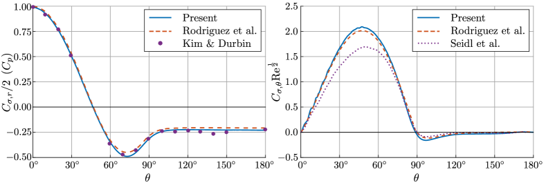
Figure 9: Time averaged pressure (left) and skin-friction (right) coefficients as functions of the polar angle, $\theta$, for a sphere at $\text{Re}=\numprint{3700}$. Results compared to values reported by Rodriguez et al. [64] (DNS at $\text{Re}=\numprint{3700}$), Kim and Durbin [65] (exp. at $\text{Re}=\numprint{4200}$), and Seidl et al. [63] (DNS at $\text{Re}=\numprint{5000}$).

Lastly, we report in Table 6 mean values for the drag coefficient ($\overline{C_{\text{D}}}$), base pressure coefficient ($\overline{C_{p}}{}_{,\text{b}}$), separation angle ($\overline{\theta_{s}}$), and polar locations of the minimum surface pressure ($\overline{\theta_{p}}{}_{,\text{min}}$) and of the maximum skin friction ($\overline{\theta_{\tau}}{}_{,\text{max}}$). With the exception of $\overline{C_{p}}{}_{,\text{b}}$, the present values are within 2.1% of those reported in [64]. The difference in $\overline{C_{p}}{}_{,\text{b}}$ is also seen to be small, i.e. approximately 2.3%, when compared to the maximum $\overline{C_{p}}$ shown in Figure 9. The value of $\overline{C_{\text{D}}}$ reported in [22] (LES) is approximately 12% lower than the $\overline{C_{\text{D}}}$ values reported here and in [64] (DNS). The grid refinement and mean turbulent statistics studies of [64] attribute this discrepancy in $\overline{C_{\text{D}}}$ value to the sub-grid model used in the numerical experiments of [22].

		Re	$\overline{C_{\text{D}}}$	$\overline{C_{p}}{}_{,\text{b}}$	$\overline{\theta_{s}}$	$\overline{\theta_{p}}{}_{,\text{min}}$	$\overline{\theta_{\tau}}{}_{,\text{max}}$
Present	DNS	$\numprint{3700}$	$0.389$	$-0.230$	$88.9^{\circ}$	$73^{\circ}$	$47^{\circ}$
YK06 [22]	LES	$\numprint{3700}$	$0.355$	$-0.194$	$90^{\circ}$	–	–
RB11 [64]	DNS	$\numprint{3700}$	$0.393$	$-0.207$	$89.3^{\circ}$	$72^{\circ}$	$48^{\circ}$
KD88 [65]	exp.	$\numprint{4200}$	–	$-0.224$	–	–	–
SM98 [63]	DNS	$\numprint{5000}$	$0.38$	–	$89.5^{\circ}$	$71^{\circ}$	$50^{\circ}$

Table 6: Mean flow features of a sphere at Reynolds numbers between $\numprint{3700}$ and $\numprint{5000}$. Results from YK06 – Yun et al. [22], RB11 – Rodriguez et al. [64], KD88 – Kim and Durbin [65], and SM98 – Seidl et al. [63] are provided.

6 Conclusions

A computationally efficient IB method for external, viscous, incompressible flows around immersed surfaces with prescribed kinematics has been presented. The IB-LGF method is a significant extension of the LGF flow solver [26], which retains the efficiency and robustness of the flow solver by coupling a Lagrange multiplier treatment of the discrete boundary forces and the discretized no-slip constraint with existing and new LGF techniques. The semi-discrete equations resulting from the formal spatial discretization of the incompressible Navier-Stokes equations on unbounded staggered Cartesian grids and the discrete delta function treatment of the IB regularization and interpolation operators is shown to constitute a DAE system of index 2. Using appropriately specialized order conditions for HERK integrators we proposed a few time integration schemes, which, when coupled with a viscous integrating factor technique, efficiently solve the discrete momentum ODE and the discrete divergence-free and no-slip constraints under a well-understood theoretical framework.

Fast flow solutions are facilitated by using a projection-like solver for the linear systems of equations arising from the implicit coupling the velocity, pressure, and boundary forces of the IF-HERK scheme. Unlike classical projection techniques, the present nested projection method is free of operator approximations, which in turn preserves the formal properties of the DAE time integration technique. This method is equivalent to a LU decomposition of the linear system and is formulated as two sequential intermediate velocity and pressure computation steps, followed by a single boundary force solution step, and finalized by two sequential pressure and velocity correction steps. Computational considerations for efficient iterative and direct boundary force solution techniques are discussed, and it is demonstrated that for many practical flows involving rigid surfaces a Cholesky-based pre-processing technique results in force solutions that require negligible computation times. The pre-processing technique results in a flow solver that depends on the solution of one additional discrete elliptic problem, i.e. force correction on the pressure, which is shown, by virtue of the flexible source and target regions of the LGF solver, to require significantly less computation time than the discrete pressure Poisson problem inherent to the flow solver (less than 50% for the numerical experiments considered).

We implemented a parallel version of the IB-LGF method for the case of rigid surfaces following the block-wise adaptive grid of the LGF flow solver. Modifications to the adaptivity criteria, grid sub-domains, and parallel load balancing procedures were performed in order to efficiently and accurately capture the flow near immersed surfaces. Detailed spatial and temporal refinement studies on flows around spheres were used to verify the expected convergence rates of the formulation. Comparisons with previous numerical investigations on flows around rectangular flat plates and spheres at Reynolds numbers up to $\numprint{3700}$ were used to confirm the physical fidelity of computed solutions. We also showed that accurate surface stresses can be obtained from the computed boundary forces using the post-processing technique of [37]. All together, the present numerical experiments have demonstrated that the IB-LGF method can overcome many of the limitations of previous IB methods including robust rigid-surface solutions, accurate and efficient unbounded domain flow solutions, physical surface stress solutions, and the feasibility of fast, accurate numerical solutions to high (based on present day DNS capabilities) Reynolds numbers flows.

Appendix A Lattice Green’s functions representations

The present formulation computes the action of $\mathsf{L}^{-1}$, $\mathsf{E}(\alpha)$, and $\mathsf{K}(\alpha)$ as discrete convolutions, e.g. Eq (7), of $\mathsf{G}_{\mathsf{L}}$, $\mathsf{G}_{\mathsf{E}}(\alpha)$, and $\mathsf{G}_{\mathsf{K}}(\alpha)$. Expressions for these LGFs in terms of Fourier and Bessel integrals are given by

$$[\mathsf{G}_{\mathsf{E}}(\alpha)](\mathbf{n}) =\frac{1}{8\pi^{3}}\int_{\Pi}e^{-i\mathbf{n}\cdot\boldsymbol{\xi}-\sigma(\boldsymbol{\xi})}\,d\boldsymbol{\xi}=\prod_{q\in\mathbf{n}}\left[e^{-2\alpha}I_{q}(2\alpha)\right],$$ (33a)

$$(\Delta x)^{2}\mathsf{G}_{\mathsf{L}}(\mathbf{n}) =\frac{1}{8\pi^{3}}\int_{\Pi}\frac{e^{-i\mathbf{n}\cdot\boldsymbol{\xi}}}{\sigma(\boldsymbol{\xi})}\,d\boldsymbol{\xi}=-\int_{0}^{\infty}[\mathsf{G}_{\mathsf{E}}(t)](\mathbf{n})\,dt,$$ (33b)

$$(\Delta x)^{2}[\mathsf{G}_{\mathsf{K}}(\alpha)](\mathbf{n}) =\frac{1}{8\pi^{3}}\int_{\Pi}\frac{e^{-i\mathbf{n}\cdot\boldsymbol{\xi}-\sigma(\boldsymbol{\xi})}}{\sigma(\boldsymbol{\xi})}\,d\boldsymbol{\xi}=-\int_{\alpha}^{\infty}[\mathsf{G}_{\mathsf{E}}(t)](\mathbf{n})\,dt,$$ (33c)

where $\sigma(\boldsymbol{\xi})=2\cos(\xi_{1})+2\cos(\xi_{2})+2\cos(\xi_{3})-6$, $\Pi=(-\pi,\pi)^{3}$, and $I_{n}(z)$ is the modified Bessel function of the first kind of order $n$.

Here, we introduce a simple procedure for efficiently computing $\left[\mathsf{G}_{\mathsf{K}}(\alpha)\right](\mathbf{n})$ and refer the reader to the discussions of [28] and [26] for examples of numerical techniques used to evaluate $\mathsf{G}_{\mathsf{L}}(\mathbf{n})$ and $[\mathsf{G}_{\mathsf{E}}(t)](\mathbf{n})$. We consider the partition of $\left[\mathsf{G}_{\mathsf{K}}(\alpha)\right](\mathbf{n})$ given by

$$\left[\mathsf{G}_{\mathsf{K}}(\alpha)\right](\mathbf{n})=\mathsf{G}_{\mathsf{L}}(\mathbf{n})+\left[\mathsf{R}(\alpha)\right](\mathbf{n}),$$ (34)

where $\left[\mathsf{R}(\alpha)\right](\mathbf{n})=(\Delta x)^{-2}\int_{0}^{\alpha}[\mathsf{G}_{\mathsf{E}}(t)](\mathbf{n})\,dt$. The combined look-up table and asymptotic expansion approach of [28] is used to compute the first term, $\mathsf{G}_{\mathsf{L}}(\mathbf{n})$, and an adaptive Gauss-Kronrod (GK) integration scheme is used to evaluate the second term, $\left[\mathsf{R}(\alpha)\right](\mathbf{n})$. For large values of $\mathbf{n}$ few, if any, subdivisions are required by the GK scheme since the value of $\left[\mathsf{R}(\alpha)\right](\mathbf{n})$ is significantly smaller than the value of $\mathsf{G}_{\mathsf{L}}(\mathbf{n})$. Lastly, we note that evaluating discrete convolution of LGFs using the LGF-FMM [28] only requires the point-wise values of LGFs to be computed once, as a pre-processing step, per simulation.

Appendix B Half-explicit Runge-Kutta schemes

The IF-HERK schemes used to perform the numerical experiments of Section 5 are:

$$\stackrel{{\scriptstyle\mbox{\small{{Scheme A}}}}}{{\begin{array}[]{c|ccc}\lx@intercol{}\hfil\lx@intercol&{}\hfil&{}\hfil&{}\hfil\\ 0&{}\hfil&{}\hfil&{}\hfil\\ \textstyle\frac{1}{2}&\textstyle\frac{1}{2}&{}\hfil&{}\hfil\\ 1&\textstyle\frac{\sqrt{3}}{3}&\textstyle\frac{3-\sqrt{3}}{3}&{}\hfil\\ \hline\cr{}\hfil&\textstyle\frac{3+\sqrt{3}}{6}&\textstyle\frac{-\sqrt{3}}{3}&\textstyle\frac{3+\sqrt{3}}{6}\end{array}}}\quad\stackrel{{\scriptstyle\mbox{\small{{Scheme B}}}}}{{\begin{array}[]{c|ccc}\lx@intercol{}\hfil\lx@intercol&{}\hfil&{}\hfil&{}\hfil\\ 0&{}\hfil&{}\hfil&{}\hfil\\ \textstyle\frac{1}{3}&\textstyle\frac{1}{3}&{}\hfil&{}\hfil\\ 1&-1&2&{}\hfil\\ \hline\cr{}\hfil&0&\textstyle\frac{3}{4}&\textstyle\frac{1}{4}\end{array}}}\quad\stackrel{{\scriptstyle\mbox{\small{{Scheme C}}}}}{{\begin{array}[]{c|ccc}\lx@intercol{}\hfil\lx@intercol&{}\hfil&{}\hfil&{}\hfil\\ 0&{}\hfil&{}\hfil&{}\hfil\\ \textstyle\frac{8}{15}&\textstyle\frac{8}{15}&{}\hfil&{}\hfil\\ \textstyle\frac{2}{3}&\textstyle\frac{1}{4}&\textstyle\frac{5}{12}&{}\hfil\\ \hline\cr{}\hfil&\textstyle\frac{1}{4}&0&\textstyle\frac{3}{4}\end{array}}}\quad\stackrel{{\scriptstyle\mbox{\small{{Scheme D}}}}}{{\begin{array}[]{c|cccc}0&{}\hfil&{}\hfil&{}\hfil&{}\hfil\\ \textstyle\frac{1}{2}&\textstyle\frac{1}{2}&{}\hfil&{}\hfil&{}\hfil\\ \textstyle\frac{1}{2}&0&\textstyle\frac{1}{2}&{}\hfil&{}\hfil\\ 1&\textstyle\frac{1}{4}&0&0&1\\ \hline\cr{}\hfil&\textstyle\frac{1}{6}&\textstyle\frac{1}{3}&\textstyle\frac{1}{3}&\textstyle\frac{1}{6}\end{array}}}$$ (55)

The expected order of accuracy for Schemes A–D based on the simplified HERK order-conditions discussed in Section 2.3 are included in Table 7. As a point of comparison, Table 7 also includes the expected order of accuracy for problems with no immersed surfaces (i.e. Eq. (8a) and (8b) with $\mathfrak{f}=0$) and for general semi-explicit DAEs of index 2 (i.e. Eq. (9)).

Scheme	$y$	$z$	$y$+	$z$+	$y$∗	$z$∗
A	2	2	2	2	2	2
B	3	2	3	2	3	2
C	2	1	3	1	2	1
D	3	1	4	1	2	1

Table 7: Expected order of accuracy of HERK schemes for the solution variable $y$ (velocity) and for the constraint variable $z$ (pressure and body forces). The superscripts $+$ and $*$ denotes values for problems with no immersed surface and for general semi-explicit DAEs of index 2, respectively.

Scheme B is the only three-stage scheme with a third-order accurate solution variable for general semi-explicit DAEs of index 2 [35]. The RK coefficients of Scheme C and Scheme D correspond to the popular three-stage fractional step method of [68] and the four-stage “original” RK method, respectively. As discussed in [26], Scheme A has the advantage of having equispaced RK nodes, i.e. $c_{i}$’s, which reduce the number of distinct integrating factors. Fewer distinct integrating factors reduces the number of pre-processing operations and lowers the storage requirements of the LGF-FMM [28] and of the Cholesky-based force Schur complement technique discussed in Section 3.2. Scheme A and D only require two distinct integrating factors (with one of them being the identity operator), as opposed to the three distinct integrating factors required by Scheme B and C.

In the absence of an immersed surface, a linear stability analysis about a uniform base flow $\mathbf{U}$ of the IF-HERK method [26] indicates that solutions are subject to the CFL condition

$$\text{CFL}=\frac{|\mathbf{U}|\Delta t}{\Delta x}<\text{CFL}_{\text{max}},$$ (56)

where $\text{CFL}_{\text{max}}$ depends on the RK coefficients of the scheme. The value of $\text{CFL}_{\text{max}}$ is unity for Schemes A–C and $\frac{2\sqrt{2}}{\sqrt{3}}$ for Scheme D. In practice, we expect solutions to the non-linear governing equations to remain stable as long as the CFL conditions resulting from linearizing the flow at each grid point are satisfied, i.e. as long as $\max(|\mathbf{u}|)\Delta t/\Delta x<\text{CFL}_{\text{max}}$.

The CFL condition $\Delta x\sim\Delta t$ and the second-order accuracy (in the absence of immersed surfaces) of the present solver imply that the potential reduction in the operation count resulting from higher than second-order HERK schemes is limited. As a result, the lower pre-processing cost of Scheme A compared to Scheme C makes Scheme A the preferred HERK scheme for the present formulation. Here, we did not consider Schemes C and D to be potential “preferred” schemes since they are only first-order accurate in the constraint variables.

References

- Peskin [2002] C. S. Peskin, The immersed boundary method, Acta numerica 11 (2002) 479–517.
- Mittal and Iaccarino [2005] R. Mittal, G. Iaccarino, Immersed boundary methods, Annual Review of Fluid Mechanics 37 (2005) 239–261.
- Hou et al. [2012] G. Hou, J. Wang, A. Layton, Numerical methods for fluid-structure interaction: a review, Communications in Computational Physics 12 (2012) 337–377.
- Peskin [1972] C. S. Peskin, Flow patterns around heart valves: a numerical method, Journal of Computational Physics 10 (1972) 252–271.
- Beyer and LeVeque [1992] R. P. Beyer, R. J. LeVeque, Analysis of a one-dimensional model for the immersed boundary method, SIAM Journal on Numerical Analysis 29 (1992) 332–364.
- Goldstein et al. [1993] D. Goldstein, R. Handler, L. Sirovich, Modeling a no-slip flow boundary with an external force field, Journal of Computational Physics 105 (1993) 354–366.
- Glowinski et al. [1998] R. Glowinski, T. W. Pan, J. Périaux, Distributed Lagrange multiplier methods for incompressible viscous flow around moving rigid bodies, Computer Methods in Applied Mechanics and Engineering 151 (1998) 181–194.
- Lai and Peskin [2000] M.-C. Lai, C. S. Peskin, An immersed boundary method with formal second-order accuracy and reduced numerical viscosity, Journal of Computational Physics 160 (2000) 705–719.
- Taira and Colonius [2007] K. Taira, T. Colonius, The immersed boundary method: a projection approach, Journal of Computational Physics 225 (2007) 2118–2137.
- Colonius and Taira [2008] T. Colonius, K. Taira, A fast immersed boundary method using a nullspace approach and multi-domain far-field boundary conditions, Computer Methods in Applied Mechanics and Engineering 197 (2008) 2131–2146.
- Kallemov et al. [2016] B. Kallemov, A. Bhalla, B. E. Griffith, A. Donev, An immersed boundary method for rigid bodies, Communications in Applied Mathematics and Computational Science 11 (2016) 79–141.
- Stein et al. [2016] D. B. Stein, R. D. Guy, B. Thomases, Immersed boundary smooth extension: A high-order method for solving PDE on arbitrary smooth domains using Fourier spectral methods, Journal of Computational Physics 304 (2016) 252–274.
- Patankar et al. [2000] N. A. Patankar, P. Singh, D. D. Joseph, R. Glowinski, T. W. Pan, A new formulation of the distributed Lagrange multiplier / fictitious domain method for particulate flows, International Journal of Multiphase Flow 26 (2000) 1509 – 1524.
- Wachs [2007] A. Wachs, Numerical simulation of steady bingham flow through an eccentric annular cross-section by distributed Lagrange multiplier / fictitious domain and augmented lagrangian methods, Journal of Non-Newtonian Fluid Mechanics 142 (2007) 183–198.
- Bhalla et al. [2013] A. P. S. Bhalla, R. Bale, B. E. Griffith, N. A. Patankar, A unified mathematical framework and an adaptive numerical method for fluid-structure interaction with rigid, deforming, and elastic bodies, Journal of Computational Physics 250 (2013) 446 – 476.
- Perot [1993] B. Perot, An analysis of the fractional step method, Journal of Computational Physics 108 (1993) 51–58.
- Chang et al. [2002] W. Chang, F. Giraldo, B. Perot, Analysis of an exact fractional step method, Journal of Computational Physics 180 (2002) 183–199.
- Tsynkov [1998] S. V. Tsynkov, Numerical solution of problems on unbounded domains. A review, Applied Numerical Mathematics 27 (1998) 465–532.
- Colonius [2004] T. Colonius, Modeling artificial boundary conditions for compressible flow, Annual Review of Fluid Mechanics 36 (2004) 315–345.
- Pradeep and Hussain [2004] D. S. Pradeep, F. Hussain, Effects of boundary condition in numerical simulations of vortex dynamics, Journal of Fluid Mechanics 516 (2004) 115–124.
- Dong et al. [2014] S. Dong, G. E. Karniadakis, C. Chryssostomidis, A robust and accurate outflow boundary condition for incompressible flow simulations on severely-truncated unbounded domains, Journal of Computational Physics 261 (2014) 83–105.
- Yun et al. [2006] G. Yun, D. Kim, H. Choi, Vortical structures behind a sphere at subcritical Reynolds numbers, Physics of Fluids 18 (2006).
- Wang and Zhang [2011] S. Wang, X. Zhang, An immersed boundary method based on discrete stream function formulation for two- and three-dimensional incompressible flows, Journal of Computational Physics 230 (2011) 3479 – 3499.
- Roma et al. [1999] A. M. Roma, C. S. Peskin, M. J. Berger, An adaptive version of the immersed boundary method, Journal of Computational Physics 153 (1999) 509 – 534.
- Griffith et al. [2007] B. E. Griffith, R. D. Hornung, D. M. McQueen, C. S. Peskin, An adaptive, formally second order accurate version of the immersed boundary method, Journal of Computational Physics 223 (2007) 10–49.
- Liska and Colonius [2016] S. Liska, T. Colonius, A fast lattice Green’s function method for solving viscous incompressible flows on unbounded domains, Accepted in Journal of Computational Physics, arXiv:1601.00035 [physics.flu-dyn] (April 2016).
- Gillman and Martinsson [2014] A. Gillman, P. G. Martinsson, A fast solver for Poisson problems on infinite regular lattices, Journal of Computational and Applied Mathematics 258 (2014) 42–56.
- Liska and Colonius [2014] S. Liska, T. Colonius, A parallel fast multipole method for elliptic difference equations, Journal of Computational Physics 278 (2014) 76–91.
- Beddhu et al. [1996] M. Beddhu, L. K. Taylor, D. L. Whitfield, Strong conservative form of the incompressible navier–stokes equations in a rotating frame with a solution procedure, Journal of Computational Physics 128 (1996) 427–437.
- Kim and Choi [2006] D. Kim, H. Choi, Immersed boundary method for flow around an arbitrarily moving body, Journal of Computational Physics 212 (2006) 662–680.
- Tsai and Colonius [2014] H.-C. Tsai, T. Colonius, Coriolis effect on dynamic stall in a vertical axis wind turbine at moderate reynolds number, in: 32nd AIAA applied aerodynamics conference, AIAA, Atlanta, GA, 2014.
- Morinishi et al. [1998] Y. Morinishi, T. S. Lund, O. V. Vasilyev, P. Moin, Fully conservative higher order finite difference schemes for incompressible flow, Journal of Computational Physics 143 (1998) 90–124.
- Zhang et al. [2002] X. Zhang, D. Schmidt, B. Perot, Accuracy and conservation properties of a three-dimensional unstructured staggered mesh scheme for fluid dynamics, Journal of Computational Physics 175 (2002) 764–791.
- Martinsson and Rodin [2002] P. G. Martinsson, G. J. Rodin, Asymptotic expansions of lattice Green’s functions, Proceedings of the Royal Society of London Series A 458 (2002) 2609–2622.
- Brasey and Hairer [1993] V. Brasey, E. Hairer, Half-explicit Runge-Kutta methods for differential-algebraic systems of index 2, SIAM Journal on Numerical Analysis 30 (1993) 538–552.
- Hairer and Wanner [1996] E. Hairer, G. Wanner, Solving ordinary differential equations II: stiff and differential-algebraic problems, Berlin Springer, 1996.
- Goza et al. [2015] A. Goza, S. Liska, B. Morley, T. Colonius, Accurate computation of surface stresses and forces with immersed boundary methods, Revised and resubmitted to Journal of Computational Physics, arXiv:1603.02306 [math-ph] (December 2015).
- Hairer et al. [1989] E. Hairer, C. Lubich, M. Roche, The numerical solution of differential-algebraic systems by Runge-Kutta methods, Lecture Notes in Mathematics, Springer-Verlag, 1989.
- Sanderse and Koren [2012] B. Sanderse, B. Koren, Accuracy analysis of explicit Runge-Kutta methods applied to the incompressible Navier-Stokes equations, Journal of Computational Physics 231 (2012) 3041–3063.
- Chori [1967] A. J. Chori, A numerical method for solving incompressible viscous flow problems, Journal of Computational Physics 2 (1967) 12–26.
- Temam [1969] R. Temam, Sur l’approximation de la solution des équations de Navier-Stokes par la méthode des pas fractionnaires (I), Archive for Rational Mechanics and Analysis 32 (1969) 135–153.
- Cao and Li [1998] Y. Cao, Q. Li, Highest order multistep formula for solving index-2 differential-algebraic equations, BIT Numerical Mathematics 38 (1998) 663–673.
- Fuhrer [2013] C. Fuhrer, Numerical Methods in Multibody Dynamics, Springer Science & Business Media, 2013.
- Blackford et al. [1997] L. S. Blackford, J. Choi, A. Cleary, E. D’Azevedo, J. Demmel, I. Dhillon, J. Dongarra, S. Hammarling, G. Henry, A. Petitet, et al., ScaLAPACK users’ guide, volume 4, SIAM, 1997.
- Shewchuk [1994] J. R. Shewchuk, An introduction to the conjugate gradient method without the agonizing pain, 1994.
- Saad [1993] Y. Saad, A flexible inner-outer preconditioned GMRES algorithm, SIAM Journal on Scientific Computing 14 (1993) 461–469.
- Chen et al. [2012] J. Chen, L. C. McInnes, H. Zhang, Analysis and practical use of flexible BiCGSTAB, Journal of Scientific Computing (2012) 1–23.
- Saff and Kuijlaars [1997] E. B. Saff, A. B. J. Kuijlaars, Distributing many points on a sphere, The Mathematical Intelligencer 19 (1997) 5–11.
- Yang et al. [2009] X. Yang, X. Zhang, Z. Li, G. W. He, A smoothing technique for discrete delta functions with application to immersed boundary method in moving boundary simulations, Journal of Computational Physics 228 (2009) 7821–7836.
- Tornberg and Engquist [2004] A.-K. Tornberg, B. Engquist, Numerical approximations of singular source terms in differential equations, Journal of Computational Physics 200 (2004) 462–488.
- Mori [2008] Y. Mori, Convergence proof of the velocity field for a Stokes flow immersed boundary method, Communications on Pure and Applied Mathematics 61 (2008) 1213–1263.
- Chen et al. [2011] K.-Y. Chen, K.-A. Feng, Y. Kim, M.-C. Lai, A note on pressure accuracy in immersed boundary method for Stokes flow, Journal of Computational Physics 230 (2011) 4377–4383.
- Tornberg and Engquist [2003] A.-K. Tornberg, B. Engquist, Regularization techniques for numerical approximation of PDEs with singularities, Journal of Scientific Computing 19 (2003) 527–552.
- Bao et al. [2015] Y.-X. Bao, J. Kaye, C. S. Peskin, A Gaussian-like immersed boundary kernel with improved translational invariance and smoothness, arXiv:1505.07529 [math.NA] (2015).
- Taira and Colonius [2009] K. Taira, T. Colonius, Three-dimensional flows around low-aspect-ratio flat-plate wings at low Reynolds numbers, Journal of Fluid Mechanics 623 (2009) 187–207.
- Wang et al. [2013] S. Wang, X. Zhang, G. He, T. Liu, A lift formula applied to low-Reynolds-number unsteady flows, Physics of Fluids 25 (2013).
- Johnson and Patel [1999] T. A. Johnson, V. C. Patel, Flow past a sphere up to a Reynolds number of 300, Journal of Fluid Mechanics 378 (1999) 19–70.
- Mittal [1999] R. Mittal, Planar symmetry in the unsteady wake of a sphere, AIAA Journal 37 (1999) 388–390.
- Tomboulides and Orszag [2000] A. G. Tomboulides, S. A. Orszag, Numerical investigation of transitional and weak turbulent flow past a sphere, Journal of Fluid Mechanics 416 (2000) 45–73.
- Ploumhans et al. [2002] P. Ploumhans, G. S. Winckelmans, J. K. Salmon, A. Leonard, M. S. Warren, Vortex methods for direct numerical simulation of three-dimensional bluff body flows: Application to the sphere at Re = 300, 500, and 1000, Journal of Computational Physics 178 (2002) 427 – 463.
- Kim et al. [2001] J. Kim, D. Kim, H. Choi, An immersed-boundary finite-volume method for simulations of flow in complex geometries, Journal of Computational Physics 171 (2001) 132 – 150.
- Constantinescu and Squires [2003] G. S. Constantinescu, K. D. Squires, LES and DES investigations of turbulent flow over a sphere at Re = 10,000, Flow, Turbulence and Combustion 70 (2003) 267–298.
- Seidl et al. [1989] V. Seidl, S. Muzaferija, M. Perić, Parallel DNS with local grid refinement, Applied Scientific Research 59 (1989) 379–394.
- Rodriguez et al. [2011] I. Rodriguez, R. Borrel, O. Lehmkuhl, C. D. Perez Segarra, A. Oliva, Direct numerical simulation of the flow over a sphere at Re = 3700, Journal of Fluid Mechanics 679 (2011) 263–287.
- Kim and Durbin [1988] H. J. Kim, P. A. Durbin, Observations of the frequencies in a sphere wake and of drag increase by acoustic excitation, Physics of Fluids 31 (1988) 3260–3265.
- Schlichting and Gersten [2003] H. Schlichting, K. Gersten, Boundary-layer theory, Springer Science & Business Media, 2003.
- Hunt et al. [1988] J. C. R. Hunt, A. A. Wray, P. Moin, Eddies, stream, and convergence zones in turbulent flows, Center for Turbulence Research CTR-S88 (1988).
- Le and Moin [1991] H. Le, P. Moin, An improvement of fractional step methods for the incompressible Navier-Stokes equations, Journal of Computational Physics 92 (1991) 369–379.