RR Lyrae stars and the horizontal branch of NGC 5904 (M5)

Abstract

We report the distance and [Fe/H] value for the globular cluster NGC 5904 (M5) derived from the Fourier decomposition of the light curves of selected RRab and RRc stars. The aim in doing this was to bring these parameters into the homogeneous scales established by our previous work on numerous other globular clusters, allowing a direct comparison of the horizontal branch luminosity in clusters with a wide range of metallicities. Our CCD photometry of the large variable star population of this cluster is used to discuss light curve peculiarities, like Blazhko modulations, on an individual basis. New Blazhko variables are reported.

From the RRab stars we found [Fe/H]${}_{\rm UVES}=-1.335\pm 0.003{\rm(statistical)}\pm 0.110{\rm(systematic)}$, and a distance of $7.6\pm 0.2$ kpc, and from the RRc stars we found [Fe/H]_UVES = $-1.39\pm 0.03{\rm(statistical)}\pm 0.12{\rm(systematic)}$ and a distance of $7.5\pm 0.3$ kpc. The results for RRab and RRc stars should be considered independent since they come from different calibrations and zero points. Absolute magnitudes, radii and masses are also reported for individual RR Lyrae stars. The distance to the cluster was also calculated by alternative methods like the Period-Luminosity relation of SX Phe and the luminosity of the stars at the tip of the red giant branch, and we obtained the results $7.7\pm 0.4$ and $7.2-7.5$ kpc respectively.

The distribution of RR Lyrae stars in the instability strip is discussed and compared with other clusters in connection with the Oosterhoff and horizontal branch type. The Oosterhoff type II clusters systematically show a RRab-RRc segregation about the instability strip first-overtone red edge, while the Oosterhoff type I clusters may or may not display this feature. A group of RR Lyrae stars is identified in an advanced evolutionary stage, and two of them are likely binaries with unseen companions.

Keywords globular clusters: individual (NGC 5904) – stars:variables: RR Lyrae, SX Phe, SR

1 Introduction

The globular cluster NGC 5904 (M5, or C1645+476 in the IAU nomenclature) ($\alpha=15^{\mbox{h}}18^{\mbox{m}}33.2^{\mbox{s}}$, $\delta=+02\arcdeg 04\arcmin 51.7\arcsec$, J2000; $l=3.85\arcdeg$, $b=+46.80\arcdeg$) is among the closest globular clusters (GCs) to the Sun and hence it is very bright. Its horizontal branch is at about $V\sim$15 mag. Being a nearby cluster, it is affected by very little reddening, $E(B-V)=0.03$ mag (Harris 1996).

M5 has a very rich population of variable stars and no doubt its proximity has contributed to the very early discovery of numerous variables. The first 46 variables were discovered by Solon J. Bailey in the last decade of the XIX century, on photographs taken with the 13-inch Boyden Telescope at Arequipa, Peru, and they were announced by Pickering (1896a). Periods of some of these variables were calculated by Pickering (1896b) and Barnard (1898). Bailey himself reported the periods for 63 of the nearly 90 variables then known (Bailey & Leland 1899) and in 1902 he listed X,Y positions for 92 variables (V1-V92, his table XXIV) and offered an identification chart (his Fig. 2, Bailey 1902). Despite the richness of the cluster in variable stars, the next batch of discoveries only happened about forty years later when Oosterhoff (1941) found V93-V103. Yet another 46 years later, Kadla et al. (1987) found the variables V104-V114. A year later variables V115-V131 were announced by Kravtsov (1988) while V132-V133 were found by Kravtsov (1991). Intense CCD photometry of the cluster led to the discovery of 35 more variables between 1996 and 2000; V134-V141 were announced by Sandquist et al. (1996) although V134 and V135 were the already known variables V129 and V36 respectively. In some cases the names of the new variables given in the original papers were modified by Caputo et al. (1999) or in the Catalogue of Variable Stars in Globular Clusters (CVSGC; Clement et al.2001) to yield a consistent list of variable names. Thus V142-143 were found by Brocato et al. (1996), V144-V148 by Reid (1996), V149-V154 by Yan & Reid (1996), V155-159 by Drissen & Shara (1998), V160-V163 by Olech et al. (1999) and V164-V168 by Kaluzny et al. (1999). V169 was noted by Rees (1993) and confirmed by Kaluzny et al. (2000). The last batch of variables, V170-V181, one SX Phe (V170) and 11 semi-regular late-type (SRA) variables, was recently announced by Arellano Ferro et al. (2015a). This makes nearly 120 years of variable star discoveries in this cluster.

As in most of our recent papers we have employed the DanDIA implementation of difference image analysis (DIA) (Bramich 2008; Bramich et al. 2013) to extract high-precision photometry for all of the point sources in the field of M5. We collected 6890 light cuves in the $V$ and $I$ bandpasses with the aim of building up a colour-magnitude diagram (CMD) and discussing the horizontal branch (HB) structure as compared to other Oosterhoff type I (OoI) and Oosterhoff type II (OoII) clusters. We also Fourier decompose the light curves of the RR Lyrae stars (RRL) to calculate their metallicity and luminosity in order to provide independent and homogeneous estimates of the cluster mean metallicity and distance.

The scheme of the paper is as follows: In $\S$ 2 we describe the observations, data reduction and calibration to the standard system. In $\S$ 3 the periods and phased light curves of RRL stars are displayed and the Fourier light curve decomposition of stable RRL is described. The corresponding individual values of [Fe/H] and $M_{V}$ are reported. $\S$ 4 deals with the discussion of the distribution of RRL in the HB. In $\S$ 5 the metallicity and distance of the parent cluster are inferred from the RRL and independent distance calculations from the P-L relation of SX Phe stars, and the luminosity of the tip of the red giant branch (TRGB). In this section we also give comments on peculiar stars. Finally, in $\S$ 6 we summarize our conclusions.

Table 1 : The distribution of observations of M5. Columns $N_{V}$ and $N_{I}$ give the number of images taken with the $V$ and $I$ filters respectively. Columns $t_{V}$ and $t_{I}$ provide the exposure time, or range of exposure times. The average seeing is listed in the last column.

Date	$N_{V}$	$t_{V}$ (s)	$N_{I}$	$t_{I}$ (s)	Avg seeing (”)
20120229	38	50-90	38	18-30	2.6
20120302	61	25-150	60	8-60	1.9
20120411	26	25-600	25	8-300	2.2
20120428	28	20-250	29	10-160	2.2
20120513	68	14-45	65	5-12	1.7
20120514	1	70	5	10-80	1.6
20120515	37	20-60	33	7-30	1.9
20130119	5	30-90	3	15-30	2.0
20130730	21	18-30	20	3-10	1.4
20140408	66	10-12	68	4-5	1.8
20140409	34	10	38	4	1.7
Total:	385		384

2 Observations and Reductions

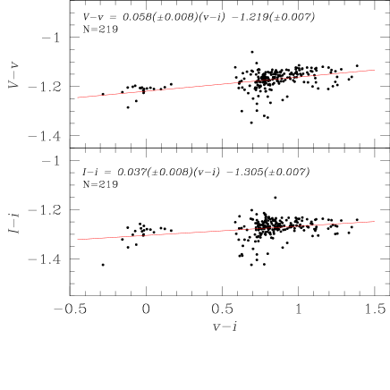
Fig. 1 : Transformation relations in the $V$ and $I$ band-passes between the instrumental and the standard photometric systems using a set of standard stars in the field of M5 (Stetson 2000).

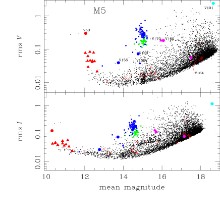
Fig. 2 : The rms magnitude deviations as a function of the mean magnitudes $V$ and $I$. Small blue and green circles represent RRab and RRc stars respectively. Other symbols are: bigger and labelled blue filled symbols for eclipsing binaries; red filled symbols for semi-regular late-type variables (SRA); purple for SX Phe stars; red crosses are stars listed in the CVSGC as variables but whose variability has not been confirmed by Arellano Ferro et al. (2015a). The U Gem variable V101 is shown as a turquoise symbol. Triangles are used for all variables discovered by Arellano Ferro et al. (2015a) where a detailed discussion on all of them can be found.

2.1 Observations

The observations were performed on 11 nights between February 29, 2012 and April 09, 2014 with the 2.0-m telescope at the Indian Astronomical Observatory (IAO), Hanle, India, located at 4500 m above sea level. A total of 385 and 384 images were obtained in the Johnson-Kron-Cousins $V$ and $I$ filters, respectively. The detector was a Thompson CCD of 2048$\times$2048 pixels with a scale of 0.296 arcsec/pix, translating to a field of view (FoV) of approximately 10.1$\times$10.1 arcmin².

The log of observations is given in Table 1 where the dates, number of frames, exposure times and average nightly seeing are recorded.

2.2 Difference Image Analysis

We employed the technique of difference image analysis (DIA) to extract high-precision photometry for all of the point sources in the images of M5 and we used the DanDIA pipeline for the data reduction process (Bramich 2008; Bramich et al. 2013). We constructed one reference image for the $V$ filter and another for the $I$ filter by stacking the best-quality images in our collection; then we created sequences of difference images in each filter by subtracting the respective convolved reference image from the rest of the collection. Differential fluxes for each star detected in the reference image were then measured on each difference image. Light curves for each star were constructed by calculating the total fluxes which in turn were converted into instrumental magnitudes. The above procedure and its caveats have been described in detail in Bramich et al. (2011), so that for brevity we do not repeat them here and refer the interested reader to that paper for further details.

Table 2 : Time-series $V$ and $I$ photometry for all the variables in our field of view. The standard $M_{\mbox{std}}$ and instrumental $m_{\mbox{ins}}$ magnitudes are listed in columns 4 and 5, respectively, corresponding to the variable star in column 1. Filter and epoch of mid-exposure are listed in columns 2 and 3, respectively. The uncertainty on $m_{\mbox{ins}}$ is listed in column 6, which also corresponds to the uncertainty on $M_{\mbox{std}}$. For completeness, we also list the quantities $f_{\mbox{ref}}$, $f_{\mbox{diff}}$ and $p$, in columns 7, 9 and 11, along with the uncertainties $\sigma_{\mbox{ref}}$ and $\sigma_{\mbox{diff}}$ in columns 8 and 10. Instrumental magnitudes are related to the other quantities via $m_{\mbox{ins}}=25.0-2.5\log(f_{\mbox{ref}}+f_{\mbox{diff}}/p)$. This is an extract from the full table, which is available only with the electronic version of the article.

Variable	Filter	HJD	$M_{\mbox{std}}$	$m_{\mbox{ins}}$	$\sigma_{m}$	$f_{\mbox{ref}}$	$\sigma_{\mbox{ref}}$	$f_{\mbox{diff}}$	$\sigma_{\mbox{diff}}$	$p$
Star ID		(d)	(mag)	(mag)	(mag)	(ADU s-1)	(ADU s-1)	(ADU s-1)	(ADU s-1)
V1	V	2455987.37467	15.391	16.588	0.003	2628.185	11.113	$-$317.143	7.107	1.0195
V1	V	2455987.37903	15.379	16.575	0.003	2628.185	11.113	$-$275.868	7.261	0.9697
⋮	⋮	⋮	⋮	⋮	⋮	⋮	⋮	⋮	⋮	⋮
V1	I	2455987.37248	14.752	16.042	0.005	4039.892	25.259	$-$222.036	19.331	1.0588
V1	I	2455987.37686	14.739	16.029	0.006	4039.892	25.259	$-$171.172	22.740	1.0423
⋮	⋮	⋮	⋮	⋮	⋮	⋮	⋮	⋮	⋮	⋮
V3	V	2455987.37467	14.938	16.128	0.002	2771.760	11.054	+780.793	7.651	1.0195
V3	V	2455987.37903	14.949	16.139	0.002	2771.760	11.054	+710.258	7.721	0.9697
⋮	⋮	⋮	⋮	⋮	⋮	⋮	⋮	⋮	⋮	⋮
V3	I	2455987.37248	14.382	15.667	0.004	4583.013	25.240	+875.643	20.340	1.0588
V3	I	2455987.37686	14.403	15.689	0.005	4583.013	25.240	+750.576	23.074	1.0423
⋮	⋮	⋮	⋮	⋮	⋮	⋮	⋮	⋮	⋮	⋮

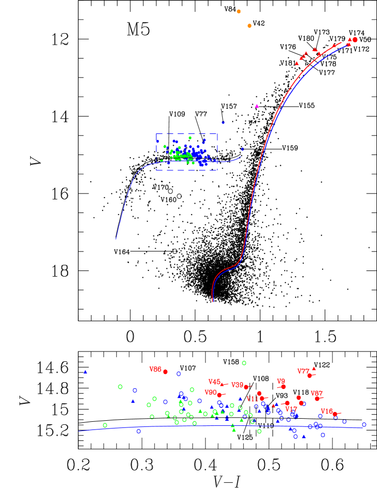
Fig. 3 : CMD of M5. In the top panel blue and green circles represent RRab and RRc stars respectively. Different colours code for other types of variables as follows: semi-regular late-type (SRA) stars red triangles; W Virginis (CW) yellow circles; SX Phe empty black circles. Some peculiar stars are labelled and discussed in $\S$ A. The isochrones of 12.0 Gyr for [Fe/H]=$-1.31$ (blue) and $-1.42$ (red) and the ZAHB models for [Fe/H]=$-1.42$, [$\alpha$/Fe]=0.4 and Y=0.25 (blue) and Y=0.27 (black) are from VandenBerg et al. (2014). The blue box containing the RR Lyrae is expanded in the lower panel, where stable stars are plotted as open circles, blue and green circles represent RRab and RRc stars, and Blazhko stars are plotted as filled triangles. Stars shown as red circles are those falling on the evolved sequence on the Period-Amplitude diagram of Fig. 6 which, along with their obvious systematically higher luminosity, identifies them as stars in a more advanced stage of evolution towards the asymptotic giant branch (AGB). Labelled stars in black digits are those displaying too short a period for their colour (Fig. 7) and probably have an unseen companion or an helium enhanced atmosphere. Stars labelled in red digits are evolved stars discussed individually in $\S$ A, those with a line segment to the right or left have increasing or decreasing periods respectively (see discussion on $\S$ 6). Three vertical dashed lines represent the empirical RRab-RRc border found (from left to right) in NGC 6229, NGC 5024 and NGC 4590 (see discussion on $\S$ 4).

2.3 Photometric Calibrations

2.3.1 Relative calibration

All photometric data suffer from systematic errors to some level that sometimes may be severe enough to be mistaken for bona fide variability in light curves. However, multiple observations of a set of objects at different epochs, such as time-series photometry, may be used to investigate, and possibly correct, these systematic errors (see for example Honeycutt 1992). This process is a relative self-calibration of the photometry, which is being performed as a standard post-processing step for large-scale surveys (e.g. Padmanabhan et al. 2008; Regnault et al. 2009).

We apply the methodology developed in Bramich & Freudling (2012) to solve for the magnitude offsets $Z_{k}$ that should be applied to each photometric measurement from the image $k$. In terms of DIA, this translates into a correction (to first order) for the systematic error introduced into the photometry from an image due to an error in the fitted value of the photometric scale factor $p$ (Bramich et al. 2015). We found that, for either filter, the magnitude offsets that we derive are of the order of $\sim 0.02$ mag and $\sim 0.03$ mag in $V$ and $I$, respectively. Applying these magnitude offsets to our DIA photometry improves the light curve quality, especially for the brighter stars.

2.3.2 Absolute calibration

Standard stars in the field of M5 are included in the online collection of Stetson (2000) and we used them to transform instrumental $vi$ magnitudes into the standard VI system.

The standard minus the instrumental magnitudes show mild dependencies on the colour, as can be seen in Fig.1. The transformations are of the form

$$V_{std}=v+0.058(\pm 0.008)(v-i)-1.219(\pm 0.007),$$ (1)

$$I_{std}=i+0.037(\pm 0.008)(v-i)-1.305(\pm 0.007).$$ (2)

All of our VI photometry for the variable stars in the FoV of our collection of images of M5 is provided in Table 2. A small portion of this table is given in the printed version of this paper and the full table is available in electronic form. Despite the fact that in the present paper we only deal with RR Lyrae and SX Phe stars, in the electronic version of the table we have also included the photometry of all variables listed in Table 3.

Fig. 2 shows the rms magnitude deviation in our $V$ and $I$ light curves, after the application of the relative photometric calibration of Section 2.3.1, as a function of the mean magnitude.

To help us discuss the variable star search and classifications, we have built the colour-magnitude diagram (CMD) of Fig. 3 by calculating the inverse-variance weighted mean magnitudes of ∼6890 stars with $V$ and $I$ magnitudes. For better precision, the periodic variables like RRL and SX Phe are plotted using their intensity-weighted magnitudes $<V>$ and colours $<V>-<I>$. The colour $<V>-<I>$ was preferred over $<V-I>$ since our $V$ and $I$ observations are not simultaneous and building up the $V-I$ colour curve would imply an undesirable interpolation process. The expansion of the HB in the bottom panel is discussed later in sections 4 and 6.

2.4 Astrometry

A linear astrometric solution was derived for the $V$ filter reference image by matching 950 hand-picked stars with the UCAC4 star catalogue (Zacharias et al. 2013) using a field overlay in the image display tool GAIA (Draper 2000). We achieved a radial RMS scatter in the residuals of $\sim$0.17 arcsec. The astrometric fit was then used to calculate the J2000.0 celestial coordinates for all of the confirmed variables in our FoV (see Table 3). The coordinates correspond to the epoch of the $V$ reference image which pertains to the average heliocentric Julian day of the six images used to form the reference image, 2456061.37 d.

Table 3 : General data for all of the variables in M5 in the FoV of our images. All variables with Blazhko modulations are labeled ’$Bl$’. Amplitudes for Blazhko variables correspond to the maximum observed.

Variable	Variable	$<V>$	$<I>$	$A_{V}$	$A_{I}$	$P$ (days)	HJDmax	RA	Dec.
Star ID	Typea	(mag)	(mag)	(mag)	(mag)	this work	(d +245 0000.)	(J2000.0)	(J2000.0)
V1	RRab $Bl^{b}$	15.165	14.639	1.06	0.70	0.521794	6757.2390	15:18:35.46	+02:07:29.5
V3	RRab	15.076	14.486	0.73	0.47	0.600189	6029.2645	15:18:44.22	+02:06:38.2
V4	RRab $Bl^{b}$	15.170	14.703	1.19	0.79	0.449647	6046.2142	15:18:32.59	+02:06:03.9
V5	RRab $Bl^{b}$	15.150	14.567	1.11	0.70	0.545853	6061.3453	15:18:32.85	+02:05:41.8
V6	RRab	15.149	14.626	0.98	0.69	0.548828	5989.4522	15:18:34.99	+02:04:02.4
V7	RRab	15.136	14.613	1.12	0.74	0.494413	5989.4323	15:18:32.52	+02:01:38.8
V8	RRab $Bl^{b}$	15.098	14.541	0.89	0.57	0.546251	5989.3293	15:18:41.95	+02:02:32.5
V9	RRab	14.907	14.343	0.77	0.51	0.698899	6063.4105	15:18:46.50	+02:06:11.5
V11	RRab	14.986	14.468	1.14	0.74	0.595897	6046.2751	15:18:23.10	+02:06:19.7
V12	RRab	15.154	14.676	1.27	0.84	0.467699	6046.2434	15:18:21.50	+02:04:38.9
V13	RRab $Bl$	15.102	14.576	1.13	0.78	0.513133	6046.2579	15:18:33.88	+02:03:44.4
V14	RRab $Bl^{b}$	15.138	14.646	1.22	0.83	0.487156	6063.2014	15:18:23.74	+02:06:38.4
V15	RRc	15.052	14.628	0.40	0.27	0.336765	6061.4425	15:18:46.13	+02:04:47.4
V16	RRab	14.911	14.374	1.21	0.79	0.647632	6756.4764	15:18:39.53	+02:06:10.6
V17	RRab	14.970	14.433	1.16	0.75	0.601390	6312.5181	15:18:31.61	+02:05:35.1
V18	RRab $Bl^{b}$	15.119	14.659	1.22	0.82	0.463961	6757.2450	15:18:43.19	+02:02:57.3
V19	RRab $Bl^{b}$	15.119	14.665	1.18	0.82	0.469999	6046.2639	15:18:48.80	+02:02:33.0
V20	RRab	15.047	14.464	0.95	0.59	0.609473	5987.4631	15:18:16.13	+02:04:34.1
V24	RRab $Bl^{b}$	15.121	14.663	1.14	0.74	0.478439	6029.3187	15:18:29.98	+02:03:40.0
V25	RRab $Bl$	15.169	14.593	0.79	0.50	0.507525	5987.3835	15:18:30.98	+02:02:42.5
V26	RRab $Bl$	15.008	14.463	1.05	0.71	0.622561	5989.4356	15:18:34.93	+02:06:30.5
V27	RRab $Bl^{b}$	15.133	14.612	0.82	0.53	0.4703217c	6063.3866	15:18:32.68	+02:03:51.1
V28	RRab $Bl$	15.114	14.561	1.12	0.71	0.543877	6312.5122	15:18:41.86	+02:02:44.8
V30	RRab $Bl^{b}$	15.085	14.497	0.82	0.54	0.592178	5987.4673	15:18:34.35	+02:01:16.3
V31	RRc	15.078	14.701	0.50	0.33	0.300580	6046.2639	15:18:43.12	+02:02:23.4
V32	RRab	15.118	14.649	1.22	0.82	0.457785	5989.4255	15:18:46.46	+02:02:13.1
V33	RRab	15.145	14.636	1.12	0.72	0.501481	5989.3506	15:18:32.11	+02:06:57.8
V34	RRab	15.127	14.567	0.83	0.57	0.568142	6061.2497	15:18:39.02	+02:05:46.6
V35	RRc $Bl$	14.959	14.607	0.48	0.29	0.308217	6063.2209	15:18:32.21	+02:02:55.7
V36	RRab	15.060	14.484	0.72	0.44	0.627725	6757.2850	15:18:32.66	+02:03:58.9
V37	RRab	15.105	14.589	1.01	0.63	0.488801	6029.3187	15:18:36.11	+02:03:41.5
V38	RRab $Bl^{b}$	15.166	14.659	1.03	0.67	0.470422	6504.2422	15:18:30.55	+02:06:48.5
V39	RRab	14.962	14.427	1.12	0.75	0.589037	6063.3327	15:18:24.35	+02:00:44.0
V40	RRc $Bl$	15.069	14.656	0.46	0.28	0.317327	6063.1929	15:18:41.85	+02:06:39.0
V41	RRab	15.110	14.619	1.29	0.83	0.488572	6061.3027	15:18:35.04	+02:08:39.9
V42	CW	11.659	10.740	1.32	0.90	25.735	6046.2397	15:18:24.80	+02:02:53.5
V43	RRab	15.029	14.428	0.56	0.43	0.660226	6757.4831	15:18:20.09	+02:07:30.9
V44	RRc $Bl$	15.091	14.633	0.45	0.26	0.329599	5987.4916	15:18:26.47	+02:05:24.4
V45	RRab $Bl$	15.042	14.471	1.01	0.66	0.616636	6061.3946	15:18:25.59	+02:05:59.5
V47	RRab	15.153	14.595	0.94	0.61	0.539730	6757.2200	15:18:28.35	+02:05:50.5
V50	SRA	12.15	10.27	0.73	0.27	107.6	6061.4267	15:18:36.04	+02:06:37.8
V52	RRab $Bl^{b}$	15.011	14.547	1.07	0.70	0.501541	6029.2645	15:18:40.56	+02:05:21.8
V53	RRc $Bl$	14.861	14.455	0.46	0.30	0.373519	5987.5209	15:18:37.92	+02:05:06.8
V54	RRab	15.183	14.718	1.27	0.90	0.454115	5989.3176	15:18:35.41	+02:05:46.0
V55	RRc $Bl$	15.086	14.634	0.41	0.26	0.328903	6504.1925	15:18:38.29	+02:02:04.1
V56	RRab $Bl^{b}$	15.127	14.585	1.01	0.69	0.534690	6061.3186	15:18:28.86	+02:06:28.6
V57	RRc	15.100	14.741	0.50	0.32	0.284697	6046.2434	15:18:31.43	+02:06:30.5
V59	RRab	15.079	14.537	0.99	0.65	0.542025	6061.2807	15:18:23.15	+02:04:19.8
V60	RRc	15.115	14.732	0.51	0.33	0.285236	6504.1518	15:18:25.94	+02:05:01.9
V61	RRab	15.113	14.544	0.92	0.61	0.568642	6061.4250	15:18:16.15	+02:04:27.7
V62	RRc	15.078	14.733	0.49	0.33	0.281417	5989.3176	15:18:43.98	+02:01:07.9
V63	RRab $Bl^{b}$	15.110	14.627	1.10	0.66	0.497686	6756.3534	15:18:47.61	+02:05:34.9
V64	RRab	15.114	14.559	0.96	0.63	0.544489	6062.1833	15:18:29.32	+02:00:42.6
V65	RRab $Bl^{b}$	15.117	14.625	1.14	0.74	0.480664	5989.4389	15:18:22.37	+02:03:21.8
V74	RRab	15.155	14.674	1.33	0.97	0.453984	6061.3915	15:18:47.19	+02:07:25.7
V77	RRab	14.744	14.148	0.57	0.44	0.845158	6061.3518	15:18:21.40	+02:01:50.9
V78	RRc	15.117	14.778	0.39	0.25	0.264820	5989.5204	15:18:37.97	+02:07:27.0
V79	RRc	15.018	14.564	0.38	0.24	0.333139	6046.2326	15:18:24.25	+02:04:22.5
V80	RRc	15.095	14.629	0.39	0.25	0.336542	6046.2751	15:18:30.24	+02:06:42.9

Table 3 : Continued

Variable	Variable	$<V>$	$<I>$	$A_{V}$	$A_{I}$	$P$ (days)	HJDmax	RA	Dec.
Star ID	Typea	(mag)	(mag)	(mag)	(mag)	this work	(d +245 0000.)	(J2000.0)	(J2000.0)
V81	RRab	15.098	14.538	0.95	0.60	0.557271	6504.2422	15:18:28.18	+02:02:50.6
V82	RRab	15.084	14.512	0.90	0.60	0.558435	6063.2014	15:18:28.76	+02:05:04.7
V83	RRab	15.122	14.572	0.86	0.59	0.553307	6061.4320	15:18:27.41	+02:03:25.0
V84	CW	11.287	10.451	0.97	0.84	26.49	6754.0000	15:18:36.13	+02:04:16.7
V85	RRab $Bl$	14.996	14.523	0.85	0.57	0.527535	6061.3804	15:18:35.75	+02:04:14.3
V86	RRab	14.944	14.439	1.24	0.87	0.567513	6504.1925	15:18:35.50	+02:04:15.9
V87	RRab	14.954	14.349	0.35	0.25	0.738421	6061.2186	15:18:41.42	+02:04:44.1
V88	RRc	15.056	14.651	0.42	0.27	0.328090	5989.5102	15:18:37.75	+02:05:49.5
V89	RRab	15.126	14.570	0.94	0.63	0.558443	6063.1970	15:18:37.41	+02:05:52.5
V90	RRab	15.027	14.496	1.30	0.84	0.557168	6061.3518	15:18:30.31	+02:05:06.7
V91	RRab	15.097	14.518	0.82	0.55	0.584945	6063.4183	15:18:30.93	+02:05:26.3
V92	RRab $Bl$	15.146	14.637	1.25	0.86	0.463388	6061.1878	15:18:29.22	+02:02:48.4
V93	RRab	15.229	14.549	1.33	0.85	0.552300	5987.4505	15:18:36.12	+02:04:13.0
V94	RRab	15.193	14.628	1.05	0.69	0.531327	6061.2497	15:18:31.71	+02:05:08.1
V95	RRc	15.050	14.675	0.50	0.35	0.290832	6061.3613	15:18:30.33	+02:06:34.0
V96	RRab	15.157	14.640	1.0	0.7	0.512255	6312.48	15:18:32.50	+02:05:23.3
V97	RRab $Bl^{b}$	15.115	14.566	0.90	0.60	0.544656	5987.3747	15:18:36.33	+02:03:16.0
V98	RRc	15.094	14.674	0.47	0.30	0.306360	6063.4216	15:18:35.81	+02:05:08.6
V99	RRc $Bl$	15.093	14.673	0.52	0.34	0.321336	6061.2186	15:18:35.57	+02:04:48.7
V100	RRc	15.146	14.769	0.50	0.33	0.294365	6504.1849	15:18:33.55	+02:05:38.6
V101	U Gem	$>19.0$	$>19.0$	–	–	–	–	15:18:14.51	+02:05:35.7
V102	RRab $Bl$	14.621	14.410	1.16	0.84	0.470540	6061.3152	15:18:34.37	+02:04:34.4
V103	RRab	15.074	14.523	0.83	0.56	0.566660	5989.4489	15:18:34.63	+02:04:40.7
V104	RRab	15.072	14.614	0.80	0.49	0.486748	6504.1830	15:18:32.68	+02:05:32.4
V105	RRc	15.234	14.957	0.58	0.48	0.295025	5987.3961	15:18:32.88	+02:05:05.5
V106	RRab $Bl$	15.192	14.703	1.25	0.96	0.527383	5987.5136	15:18:32.93	+02:04:59.5
V107	RRab	14.932	14.419	1.03	0.69	0.511698	5987.4799	15:18:33.25	+02:04:46.0
V108	RRc	14.980	14.517	0.48	0.31	0.328628	5989.5204	15:18:33.79	+02:04:47.0
V109	RRab	15.549	14.992	2.0	1.4	0.473008	6046.3241	15:18:34.57	+02:04:50.8
V110	RRab	15.254	14.706	0.72	0.54	0.597996	6312.5083	15:18:34.88	+02:04:45.7
V111	RRab	15.074	14.470	0.85	0.50	0.634647	5989.4221	15:18:34.89	+02:05:05.5
V112	RRab $Bl$	15.074	14.592	0.8	0.6	0.534456	5989.3749	15:18:35.11	+02:04:17.4
V113	RRc	15.101	14.726	0.5	0.3	0.284676	5989.3541	15:18:35.12	+02:04:15.2
V114	RRab	15.167	14.592	0.84	0.58	0.603659	6504.1668	15:18:35.24	+02:04:46.5
V115	RRab	15.045	14.445	0.59	0.41	0.609084	5989.3644	15:18:36.33	+02:04:53.8
V116	RRc	14.972	14.579	0.47	0.31	0.347289	5987.5209	15:18:36.33	+02:04:46.1
V117	RRc	14.951	14.512	0.35	0.24	0.335929	6061.4320	15:18:34.90	+02:04:52.2
V118	RRab	14.870	14.294	1.16	0.71	0.580517	6063.2638	15:18:34.59	+02:04:57.0
V119	RRab	15.171	14.531	0.94	0.58	0.550962	6504.2405	15:18:34.13	+02:05:05.1
V120	RRc $Bl$	15.154	14.737	0.58	0.39	0.278719	5989.5137	15:18:33.83	+02:04:57.6
V121	RRab $Bl$	15.348	14.623	1.15	0.66	0.599039	6063.2528	15:18:32.93	+02:04:43.0
V122	RRab $Bl$	14.682	14.077	0.64	0.51	0.733089	5987.4589	15:18:32.02	+02:04:45.1
V123	RRab	15.167	14.530	0.68	0.45	0.602486	6504.1686	15:18:33.26	+02:05:18.8
V125	RRc	15.098	14.594	0.44	0.28	0.303304	6063.2865	15:18:32.17	+02:05:06.8
V126	RRc	15.147	14.659	0.45	0.40	0.343258	5989.3506	15:18:32.06	+02:05:02.2
V127	RRab $Bl$	14.673	14.548	0.81	0.77	0.540366	5987.4839	15:18:30.76	+02:05:00.8
V128	RRc	15.109	14.709	0.48	0.32	0.306013	5989.4122	15:18:30.81	+02:04:42.5
V129	RRab	15.136	14.574	0.59	0.41	0.605302	6504.2332	15:18:30.05	+02:04:01.7
V130	RRc $Bl$	14.993	14.605	0.6	0.4	0.327187	6046.2288	15:18:38.59	+02:05:44.7
V131	RRc $Bl$	15.149	14.774	0.6	0.4	0.281533	6046.2326	15:18:38.60	+02:05:42.2
V132	RRc	15.035	14.678	0.38	0.26	0.283738	6029.4767	15:18:36.28	+02:05:33.8
V133	RRc	14.989	14.606	0.47	0.28	0.294864	5987.3747	15:18:40.53	+02:05:30.1
V137	RRab	15.159	14.558	0.50	0.36	0.619359	6063.2901	15:18:36.33	+02:05:28.8
V139	RRc	14.796	14.517	0.37	0.26	0.300356	6504.1518	15:18:32.09	+02:05:22.8
V142	RRab $Bl$	15.087	14.714	1.4	1.0	0.458151	6029.3187	15:18:34.48	+02:04:50.2
V155	EW	13.74	12.76	0.14	0.09	0.664865	6504.2067	15:18:33.40	+02:05:12.2

Table 3 : Continued

Variable	Variable	$<V>$	$<I>$	$A_{V}$	$A_{I}$	$P$ (days)	HJDmax	RA	Dec.
Star ID	Typea	(mag)	(mag)	(mag)	(mag)	this work	(d +245 0000.)	(J2000.0)	(J2000.0)
V156	RRab d	12.912	11.721	0.18	–	–	–	15:18:32.63	+02:04:59.0
V157	RRab	14.140	13.434	0.60	–	0.517608	6063.2014	15:18:33.37	+02:04:58.0
V158	RRc	14.580	14.106	0.45	0.31	0.442627	5989.4752	15:18:32.83	+02:04:50.6
V159	E	14.85	13.99	–	–	–	–	15:18:32.88	+02:04:36.5
V160	SX Phe	16.05	15.70	0.55	0.34	0.089749	5989.5102	15:18:29.84	+02:04:09.8
V161	RRc	15.161	14.702	0.42	0.26	0.331266	6046.2468	15:18:33.71	+02:05:41.5
V164	SX Phe	17.50	17.15	0.15	–	0.042134	6029.4832	15:18:22.77	+02:02:49.3
V170	SX Phe	15.95	15.63	0.57	0.41	0.089467	6063.3361	15:18:32.14	+02:04:20.4
V171	SRA	12.17	10.50	0.25	0.14	28.8	6312.5083	15:18:34.26	+02:04:24.2
V172	SRA	12.15	10.47	0.23	0.13	–	–	15:18:31.59	+02:04:41.4
V173	SRA	12.28	10.86	0.13	0.13	43.1	6504.1686	15:18:28.42	+02:04:29.8
V174	SRA	12.03	10.33	0.33	0.15	80.6	6063.4183	15:18:34.18	+02:06:25.5
V175	SRA	12.40	10.94	0.18	0.13	–	–	15:18:36.22	+02:05:11.3
V176	SRA	12.46	11.13	0.22	0.20	133.3	5989.3064	15:18:37.38	+02:06:08.2
V177	SRA	12.51	11.19	0.13	0.10	–	–	15:18:41.40	+02:06:00.9
V178	SRA	12.39	11.03	0.12	0.10	141.6	5987.4759	15:18:33.10	+02:04:58.0
V179	SRA	12.18	10.61	0.12	0.11	–	–	15:18:33.42	+02:04:59.6
V180	SRA	12.27	10.86	0.24	0.24	–	–	15:18:35.82	+02:03:42.4
V181	SRA	12.64	11.36	0.07	0.08	–	–	15:18:45.40	+02:04:30.9

Fig. 4 : Light curves of the RRab stars in M5. To preserve the vertical scale and limits, the vertical axes display $V-<V>$ and $I-<I>$. All light curves are phased with the ephemerides listed in Table 3. Individual mean values and amplitudes are also listed in the table.

Fig. 4 : Continued

Fig. 4 : Continued

Fig. 5 : Light curves of the RRc stars in M5 phased with the ephemerides listed in Table 3.

Fig. 5 : Continued

3 The RR Lyrae stars in M5

The $V$ and $I$ light curves of 79 RRab and 34 RRc stars in the FoV of our images are displayed in Figs. 4 and 5. Note that the variables V2, V10, V21, V22, V29, V58, V66-V73, V75, V76, V141 and V165-V169 are outside the FoV of our study. We do not plot the RRab star V156 in Figure 4 because we were unable to phase our light curve, although we confirm that it is variable (see the comment in $\S$ A and the light curve in Fig.11). The stars in Figs. 4 and 5 are discussed individually in $\S$ A when found peculiar. The RR Lyrae stars were selected for the Fourier decomposition approach for the determination of their physical parameters only when their light curves are considered sufficiently stable, i.e. with no clear signs of amplitude modulations.

3.1 Periods

The light curves of the RRab and RRc stars in Figs. 4 and 5 were phased with the ephemerides in Table 3.

The periods reported in Table 3 were calculated exclusively on our data from 2012-2014, applying the string-length method (Burke, Rolland & Boy 1970; Dworetsky 1983) as well as period04 (Lenz & Breger 2005). It is well known, however, from the pioneering work of Oosterhoff (1941) to the most recent analysis by Szeidl et al. (2011), that most RRL in M5 do exhibit secular period variations, thus the periods given in Table 3 are not likely to be the most precise ones. Nevertheless, they are instantaneous accurate values that phase the light curves during 2012-2014 very well, as can be judged from the phased light curves in Figs. 4 and 5, and that can be accurately used to Fourier decompose the light curves in pursuit of physical parameters, as will be described later in this paper. In a separate paper we shall revisit the secular period change nature of the RRL in M5 in the light of our observations which extend the time-base by at least 15 years.

3.2 [Fe/H] and M_V from light curve Fourier decomposition

Stellar physical parameters, such as [Fe/H], M_V, $T_{\rm eff}$, mass and radius for RRL can be calculated via the Fourier decomposition of their $V$ light curves into its harmonics as:

$$m(t)=A_{0}~{}+~{}\sum_{k=1}^{N}{A_{k}~{}\cos~{}({2\pi\over P}~{}k~{}(t-E)~{}+~{}\phi_{k})},$$ (3)

where $m(t)$ is the magnitude at time $t$, $P$ is the period and $E$ the epoch. A linear minimization routine is used to derive the amplitudes $A_{k}$ and phases $\phi_{k}$ of each harmonic, from which the Fourier parameters $\phi_{ij}=j\phi_{i}-i\phi_{j}$ and $R_{ij}=A_{i}/A_{j}$ are calculated. The mean magnitudes $A_{0}$, and the Fourier light curve fitting parameters of individual RRab and RRc stars are listed in Table  4. In this table we have excluded stars with evident amplitude-phase modulations, excessive noise, apparent blending or incomplete light curves that badly disturbed the Fourier fit. The latter case is particularly true in those light curves where the maximum or minimum are missing.

Table 4 : Fourier coefficients $A_{k}$ for $k=0,1,2,3,4$, and phases $\phi_{21}$, $\phi_{31}$ and $\phi_{41}$, for RRab and RRc stars. The numbers in parentheses indicate the uncertainty on the last decimal place. Also listed is the deviation parameter $D_{\mbox{m}}$ (see Section 3.2).

Variable ID	$A_{0}$	$A_{1}$	$A_{2}$	$A_{3}$	$A_{4}$	$\phi_{21}$	$\phi_{31}$	$\phi_{41}$	$D_{\mbox{m}}$
	($V$ mag)	($V$ mag)	($V$ mag)	($V$ mag)	($V$ mag)
					RRab stars
V3	15.076(1)	0.245(2)	0.120(1)	0.082(2)	0.041(1)	4.063(18)	8.486(25)	6.758(42)	1.1
V5	15.150(1)	0.367(1)	0.182(1)	0.129(1)	0.087(1)	3.942(8)	8.231(12)	6.223(17)	2.2
V6	15.149(1)	0.338(2)	0.165(2)	0.117(2)	0.079(1)	3.911(13)	8.215(18)	6.204(28)	1.5
V7	15.136(2)	0.380(2)	0.180(2)	0.139(2)	0.095(2)	3.797(17)	7.916(23)	5.836(33)	0.5
V9	14.907(1)	0.279(1)	0.133(1)	0.089(1)	0.038(1)	4.234(11)	8.755(17)	7.068(33)	3.1
V11	14.986(1)	0.373(1)	0.204(1)	0.130(1)	0.091(1)	4.043(9)	8.356(14)	6.507(18)	2.5
V12	15.154(2)	0.429(2)	0.199(2)	0.153(2)	0.104(2)	3.824(15)	7.915(20)	5.827(27)	1.3
V16	14.911(2)	0.401(3)	0.218(3)	0.134(3)	0.092(2)	4.130(15)	8.418(22)	6.751(34)	4.8
V17	14.970(1)	0.387(1)	0.207(1)	0.129(1)	0.094(1)	3.998(7)	8.274(11)	6.413(15)	2.3
V20	15.047(1)	0.306(1)	0.164(1)	0.108(2)	0.067(1)	4.139(12)	8.584(18)	6.851(28)	2.1
V30	15.085(1)	0.268(2)	0.140(2)	0.094(2)	0.053(2)	3.985(16)	8.377(24)	6.551(38)	1.0
V32	15.118(1)	0.419(2)	0.198(2)	0.146(2)	0.093(2)	3.850(13)	7.862(18)	5.804(26)	1.6
V33	15.145(1)	0.382(2)	0.175(2)	0.136(2)	0.090(2)	3.794(15)	7.905(19)	5.763(28)	4.1
V34	15.127(1)	0.288(1)	0.138(1)	0.093(2)	0.055(1)	3.988(15)	8.295(20)	6.413(31)	1.1
V38	15.166(1)	0.382(2)	0.174(2)	0.114(2)	0.071(2)	3.843(12)	7.982(19)	5.980(28)	1.3
V39	14.962(1)	0.374(1)	0.198(1)	0.127(1)	0.090(1)	3.984(8)	8.264(12)	6.316(17)	1.6
V41	15.110(1)	0.444(1)	0.209(1)	0.157(1)	0.101(2)	3.803(9)	7.973(13)	5.858(18)	1.2
V54	15.183(1)	0.451(2)	0.206(2)	0.154(2)	0.098(2)	3.786(10)	7.886(15)	5.832(21)	1.8
V59	15.079(1)	0.327(1)	0.169(1)	0.114(1)	0.079(1)	3.949(9)	8.265(14)	6.279(19)	0.9
V61	15.113(1)	0.312(1)	0.156(1)	0.105(1)	0.071(1)	4.005(11)	8.335(17)	6.433(24)	1.8
V64	15.114(1)	0.320(1)	0.157(1)	0.112(1)	0.076(1)	3.894(12)	8.167(17)	6.152(24)	0.9
V74	15.155(1)	0.447(2)	0.208(2)	0.159(2)	0.106(2)	3.883(15)	8.007(21)	5.916(29)	1.2
V77	14.744(1)	0.226(1)	0.089(2)	0.036(2)	0.022(2)	4.528(23)	9.270(50)	7.521(74)	4.8
V81	15.098(1)	0.314(1)	0.157(1)	0.111(1)	0.071(1)	3.936(10)	8.260(14)	6.299(21)	1.6
V82	15.084(1)	0.307(1)	0.152(1)	0.107(1)	0.068(1)	3.941(9)	8.262(13)	6.321(19)	1.8
V83	15.122(1)	0.291(2)	0.146(2)	0.104(2)	0.064(2)	3.956(15)	8.291(22)	6.343(32)	0.9
V86	14.944(1)	0.419(2)	0.222(2)	0.137(2)	0.104(2)	3.872(11)	8.191(17)	6.145(23)	2.7
V89	15.126(1)	0.321(1)	0.162(1)	0.112(1)	0.072(1)	3.973(8)	8.291(12)	6.355(17)	1.6
V90	15.027(1)	0.448(1)	0.227(2)	0.149(2)	0.102(2)	3.904(9)	8.232(14)	6.157(18)	1.9
V91	15.097(1)	0.281(1)	0.144(1)	0.098(1)	0.057(1)	4.044(11)	8.409(16)	6.507(24)	0.8
V94	15.193(2)	0.360(3)	0.178(3)	0.131(4)	0.084(3)	3.842(25)	8.164(33)	6.055(48)	2.2
V103	15.074(2)	0.292(2)	0.146(2)	0.106(2)	0.052(2)	3.909(20)	8.285(29)	6.421(49)	2.2
V107	14.932(1)	0.345(2)	0.168(2)	0.132(2)	0.081(2)	3.784(15)	7.905(21)	5.710(20)	1.7
V110	15.254(1)	0.259(2)	0.117(2)	0.084(2)	0.040(2)	4.222(20)	8.744(29)	7.024(52)	3.9
V114	15.167(1)	0.285(1)	0.134(1)	0.094(1)	0.052(1)	4.056(15)	8.336(22)	6.549(34)	1.8
V118	14.870(2)	0.386(2)	0.208(2)	0.134(2)	0.093(2)	4.018(14)	8.354(21)	6.234(32)	3.7
V119	15.171(1)	0.311(2)	0.156(2)	0.110(2)	0.073(2)	3.929(15)	8.200(22)	6.286(32)	0.8
V123	15.167(1)	0.244(1)	0.117(1)	0.074(1)	0.035(1)	4.118(15)	8.528(23)	6.817(42)	0.7
					RRc stars
V15	15.052(1)	0.204(1)	0.023(1)	0.015(1)	0.006(1)	5.156(43)	3.893(64)	2.938(160)	–
V31	15.078(1)	0.252(1)	0.042(1)	0.023(1)	0.018(1)	4.589(24)	2.822(43)	1.658(54)	–
V55	15.086(1)	0.199(1)	0.024(1)	0.013(1)	0.007(1)	4.567(55)	3.322(104)	2.105(192)	–
V57	15.100(1)	0.251(1)	0.044(1)	0.018(1)	0.017(1)	4.769(18)	2.853(42)	1.471(46)	–
V60	15.115(1)	0.252(1)	0.045(1)	0.022(1)	0.017(1)	4.639(24)	2.683(49)	1.570(60)	–
V62	15.078(1)	0.240(1)	0.045(1)	0.020(1)	0.016(1)	4.531(37)	2.818(81)	1.409(102)	–
V78	15.117(1)	0.197(1)	0.029(1)	0.007(1)	0.006(1)	4.636(30)	2.680(128)	1.464(154)	–
V79	15.018(1)	0.190(1)	0.019(1)	0.008(1)	0.004(1)	4.607(47)	4.121(117)	3.167(210)	–
V80	15.095(1)	0.201(1)	0.013(1)	0.015(1)	0.006(1)	4.979(92)	3.870(79)	2.480(196)	–
V88	15.056(1)	0.212(1)	0.024(1)	0.018(1)	0.006(1)	4.582(49)	3.430(64)	2.720(193)	–
V95	15.050(1)	0.245(1)	0.042(1)	0.020(1)	0.020(1)	4.763(28)	2.900(60)	1.532(60)	–
V98	15.094(1)	0.232(1)	0.033(1)	0.019(1)	0.008(1)	4.582(40)	3.164(68)	2.241(152)	–
V100	15.146(1)	0.252(1)	0.040(1)	0.023(1)	0.016(1)	4.688(34)	2.906(62)	1.771(85)	–
V105	15.234(2)	0.297(3)	0.049(4)	0.032(4)	0.028(4)	4.733(75)	2.972(116)	1.788(136)	–
V108	14.980(1)	0.236(2)	0.020(2)	0.012(2)	0.010(2)	4.894(101)	3.537(166)	2.715(192)	–
V113	15.101(2)	0.263(2)	0.053(2)	0.020(2)	0.020(2)	4.799(44)	3.022(112)	1.338(114)	–
V116	14.972(1)	0.238(1)	0.021(1)	0.017(1)	0.012(1)	4.861(43)	3.898(53)	2.537(77)	–
V117	14.951(1)	0.169(2)	0.018(2)	0.011(2)	0.001(2)	5.344(114)	3.601(192)	3.233(355)	–
V125	15.098(2)	0.229(2)	0.028(2)	0.021(2)	0.012(2)	4.816(82)	3.284(111)	2.270(200)	–
V128	15.109(1)	0.243(2)	0.034(2)	0.025(2)	0.015(2)	4.635(46)	3.358(61)	2.360(103)	–
V132	15.035(1)	0.191(1)	0.026(1)	0.010(1)	0.008(1)	4.654(53)	2.908(129)	1.255(296)	–
V133	14.989(1)	0.225(1)	0.034(1)	0.018(1)	0.014(1)	4.912(43)	3.202(81)	1.910(101)	–
V139	14.796(1)	0.185(1)	0.026(1)	0.017(1)	0.010(1)	4.705(43)	2.950(65)	1.610(110)	–
V161	15.161(1)	0.209(2)	0.023(2)	0.011(1)	0.005(1)	4.777(66)	3.556(145)	2.652(296)	–

These Fourier parameters and the semi-empirical calibrations of Jurcsik & Kovács (1996), for RRab stars, and Morgan, Wahl & Wieckhorts (2007), for RRc stars, are used to obtain [Fe/H]_ZW on the Zinn & West (1984) metallicity scale which have been transformed to the UVES scale using the equation [Fe/H]_UVES= $-0.413$ +0.130[Fe/H]${}_{\rm ZW}-0.356$[Fe/H]${}_{\rm ZW}^{2}$ (Carretta et al. 2009). The absolute magnitude $M_{V}$ can be derived from the calibrations of Kovács & Walker (2001) for RRab stars and of Kovács (1998) for the RRc stars. The effective temperature $T_{\rm eff}$ was estimated using the calibration of Jurcsik (1998). For brevity we do not explicitly present here the above mentioned calibrations; however, the corresponding equations, and most importantly their zero points, have been discussed in detail in previous papers (e.g. Arellano Ferro et al. 2011; 2013) and the interested reader is referred to them.

Let us recall that the calibration for [Fe/H] for RRab stars of Jurcsik & Kovács (1996) is applicable to RRab stars with a deviation parameter $D_{m}$, defined by Jurcsik & Kovács (1996) and Kovács & Kanbur (1998), not exceeding an upper limit. These authors suggest $D_{m}\leq 3.0$. The $D_{m}$ is listed in column 10 of Table 4. However we have relaxed the criterion to include six stars with 3.0 $\leq D_{m}\leq$ 4.8. The RRab V25 and V157, which are likely blended in our images, are not included in the Fourier decomposition analysis. They are addressed in $\S$ A.

Table 5 : Physical parameters for the RRab and RRc stars. The numbers in parentheses indicate the uncertainty on the last decimal place.

Star	[Fe/H]ZW	[Fe/H]UVES	$M_{V}$	log $T_{\rm eff}$	log$(L/{\rm L_{\odot}})$	$M/{\rm M_{\odot}}$	$R/{\rm R_{\odot}}$
			RRab stars
V3	$-1.375(23)$	$-1.265(23)$	0.610(3)	3.805(8)	1.656(1)	0.64(6)	5.55(1)
V5	$-1.410(11)$	$-1.304(11)$	0.584(1)	3.813(7)	1.666(1)	0.68(6)	5.40(1)
V6	$-1.436(17)$	$-1.333(17)$	0.603(3)	3.812(8)	1.659(1)	0.68(6)	5.39(1)
V7	$-1.512(22)$	$-1.423(23)$	0.658(3)	3.816(8)	1.637(1)	0.71(7)	5.16(1)
V9	$-1.494(16)$	$-1.402(17)$	0.452(1)	3.797(8)	1.719(1)	0.67(6)	6.18(1)
V11	$-1.480(13)$	$-1.386(14)$	0.507(1)	3.808(7)	1.697(1)	0.70(6)	5.73(1)
V12	$-1.412(19)$	$-1.306(19)$	0.658(3)	3.821(8)	1.637(1)	0.72(6)	5.05(1)
V16	$-1.617(21)$	$-1.555(24)$	0.410(4)	3.802(8)	1.736(2)	0.74(7)	6.16(1)
V17	$-1.578(10)$	$-1.505(12)$	0.482(1)	3.807(7)	1.707(1)	0.72(6)	5.83(1)
V20	$-1.317(17)$	$-1.202(16)$	0.547(2)	3.807(8)	1.681(1)	0.65(6)	5.66(1)
V30	$-1.447(23)$	$-1.347(23)$	0.603(3)	3.806(8)	1.659(1)	0.65(6)	5.55(1)
V32	$-1.424(17)$	$-1.320(17)$	0.682(3)	3.821(7)	1.627(1)	0.73(6)	4.99(1)
V33	$-1.548(18)$	$-1.468(20)$	0.641(3)	3.815(8)	1.643(1)	0.71(6)	5.21(1)
V34	$-1.434(19)$	$-1.331(19)$	0.613(2)	3.808(8)	1.655(1)	0.66(6)	5.45(1)
V38	$-1.359(18)$	$-1.247(17)$	0.675(3)	3.819(8)	1.630(1)	0.72(6)	5.04(1)
V39	$-1.541(11)$	$-1.459(12)$	0.512(1)	3.808(7)	1.695(1)	0.71(6)	5.71(1)
V41	$-1.436(12)$	$-1.334(13)$	0.608(1)	3.820(7)	1.657(1)	0.73(6)	5.19(1)
V54	$-1.388(14)$	$-1.279(14)$	0.657(3)	3.822(7)	1.637(1)	0.74(6)	5.01(1)
V59	$-1.363(13)$	$-1.252(13)$	0.623(1)	3.813(7)	1.651(1)	0.66(6)	5.31(1)
V61	$-1.398(16)$	$-1.291(16)$	0.596(1)	3.810(7)	1.662(1)	0.66(6)	5.47(1)
V64	$-1.464(16)$	$-1.367(17)$	0.626(1)	3.811(7)	1.649(1)	0.67(6)	5.35(1)
V74	$-1.274(20)$	$-1.156(18)$	0.666(3)	3.824(8)	1.633(1)	0.72(7)	4.95(1)
V77	$-1.562(47)$	$-1.484(53)$	0.315(2)	3.786(11)	1.774(1)	0.68(9)	6.93(1)
V81	$-1.426(13)$	$-1.322(13)$	0.614(1)	3.810(7)	1.654(1)	0.66(6)	5.40(1)
V82	$-1.428(12)$	$-1.324(13)$	0.617(1)	3.810(7)	1.653(1)	0.66(6)	5.40(1)
V83	$-1.381(21)$	$-1.272(21)$	0.641(3)	3.811(8)	1.644(1)	0.65(6)	5.33(1)
V86	$-1.529(16)$	$-1.443(18)$	0.499(3)	3.812(7)	1.700(1)	0.73(6)	5.65(1)
V89	$-1.401(11)$	$-1.294(11)$	0.606(1)	3.811(7)	1.658(1)	0.67(6)	5.41(1)
V90	$-1.452(13)$	$-1.352(14)$	0.490(2)	3.815(7)	1.704(1)	0.73(6)	5.60(1)
V91	$-1.389(15)$	$-1.281(15)$	0.603(1)	3.808(7)	1.659(1)	0.65(6)	5.49(1)
V94	$-1.418(31)$	$-1.313(32)$	0.616(5)	3.815(9)	1.654(2)	0.68(7)	5.29(1)
V103	$-1.437(27)$	$-1.335(28)$	0.622(3)	3.808(9)	1.651(1)	0.66(7)	5.43(1)
V107	$-1.587(20)$	$-1.516(22)$	0.665(3)	3.813(7)	1.634(1)	0.69(6)	5.21(1)
V110	$-1.124(27)$	$-1.009(22)$	0.598(3)	3.809(9)	1.661(1)	0.62(7)	5.47(1)
V114	$-1.529(21)$	$-1.444(23)$	0.568(1)	3.804(8)	1.673(1)	0.67(6)	5.69(1)
V118	$-1.424(20)$	$-1.321(20)$	0.517(3)	3.812(8)	1.693(1)	0.68(6)	5.60(1)
V119	$-1.458(21)$	$-1.359(22)$	0.626(3)	3.810(8)	1.650(1)	0.67(6)	5.38(1)
V123	$-1.344(22)$	$-1.231(21)$	0.601(1)	3.805(8)	1.660(1)	0.64(6)	5.57(1)
Weighted
Mean	$-1.444(3)$	$-1.335(3)$	0.575(1)	3.811(1)	1.670(1)	0.68(1)	5.49(1)
			RRc stars
V15	$-1.45(13)$	$-1.35(13)$	0.553(2)	3.865(0)	1.679(1)	0.51(0)	4.32(1)
V31	$-1.62(8)$	$-1.56(09)$	0.559(1)	3.866(0)	1.676(0)	0.59(0)	4.28(1)
V55	$-1.67(20)$	$-1.62(24)$	0.582(5)	3.863(1)	1.667(2)	0.52(5)	4.30(1)
V57	$-1.43(7)$	$-1.32(07)$	0.571(1)	3.870(0)	1.672(0)	0.60(0)	4.19(1)
V60	$-1.52(8)$	$-1.43(09)$	0.575(1)	3.869(0)	1.670(0)	0.61(0)	4.20(1)
V62	$-1.41(14)$	$-1.30(14)$	0.589(2)	3.870(0)	1.665(1)	0.60(0)	4.15(1)
V78	$-1.27(21)$	$-1.15(19)$	0.647(1)	3.873(1)	1.641(1)	0.59(1)	3.98(1)
V79	$-1.26(24)$	$-1.15(22)$	0.588(2)	3.867(1)	1.665(1)	0.49(0)	4.21(1)
V80	$-1.46(16)$	$-1.36(17)$	0.559(4)	3.865(0)	1.676(2)	0.51(0)	4.31(1)
V88	$-1.61(12)$	$-1.55(14)$	0.588(2)	3.864(0)	1.665(1)	0.52(0)	4.27(1)
V95	$-1.48(10)$	$-1.38(11)$	0.553(1)	3.869(0)	1.679(0)	0.61(0)	4.25(1)
V98	$-1.52(12)$	$-1.43(13)$	0.597(2)	3.867(0)	1.661(1)	0.55(0)	4.20(1)
V100	$-1.51(11)$	$-1.43(12)$	0.571(1)	3.868(0)	1.672(1)	0.59(0)	4.23(1)
V105	$-1.49(20)$	$-1.39(22)$	0.514(3)	3.868(1)	1.694(1)	0.62(1)	4.33(1)
V108	$-1.56(32)$	$-1.48(36)$	0.554(4)	3.865(1)	1.678(2)	0.53(1)	4.33(1)
V113	$-1.33(20)$	$-1.22(19)$	0.556(2)	3.871(1)	1.678(1)	0.61(1)	4.20(1)
V116	$-1.56(11)$	$-1.48(12)$	0.530(2)	3.863(0)	1.688(1)	0.51(0)	4.40(1)
V117	$-1.60(38)$	$-1.54(43)$	0.568(19)	3.864(1)	1.673(4)	0.51(1)	4.32(2)
V125	$-1.42(20)$	$-1.31(21)$	0.575(4)	3.868(1)	1.670(1)	0.56(1)	4.21(1)

Table 5 : Continued

Star	[Fe/H]ZW	[Fe/H]UVES	$M_{V}$	log $T_{\rm eff}$	log$(L/{\rm L_{\odot}})$	$M/{\rm M_{\odot}}$	$R/{\rm R_{\odot}}$
V128	$-1.41(11)$	$-1.30(11)$	0.566(2)	3.868(0)	1.674(1)	0.56(0)	4.23(1)
V132	$-1.39(22)$	$-1.28(22)$	0.616(2)	3.870(1)	1.654(1)	0.57(1)	4.09(1)
V133	$-1.36(15)$	$-1.25(14)$	0.568(2)	3.870(0)	1.673(1)	0.58(0)	4.20(1)
V139	$-1.56(12)$	$-1.48(13)$	0.590(2)	3.867(0)	1.664(1)	0.57(0)	4.21(1)
V161	$-1.58(28)$	$-1.51(32)$	0.578(3)	3.864(1)	1.669(1)	0.51(1)	4.29(1)
Weighted
Mean	$-1.49(3)$	$-1.39(3)$	0.578(1)	3.867(1)	1.669(1)	0.56(1)	4.22(1)

The physical parameters for the RRL and the inverse-variance weighted means are reported in Table 5. Two independent estimations of [Fe/H]_UVES were found from 38 RRab and 24 RRc stars in M5: $-1.34\pm 0.11$ and $-1.39\pm 0.12$ respectively, where the uncertainties are the standard deviations of the inverse-variance weighted means.

Morgan (2013) published a new calibration of [Fe/H]_UVES for RRc stars, calculated for an extended number of stars and clusters, and noted that the results of the new calibration are in general consistent with the old one from Morgan et al. (2007), and that the average differences are of the order of 0.02 dex. We have also carried out the calculation using the new calibration and found [Fe/H]${}_{\rm UVES}=-1.43$, i.e. 0.04 dex more deficient than the value derived with the calibration of Morgan et al. (2007) which is in better agreement with the result from the RRab calibration. A similar conclusion was found by Arellano Ferro et al. (2015b) for the case of NGC 6229.

The weighted mean $M_{V}$ values for the RRab and RRc stars are 0.575$\pm$0.082 mag and 0.578$\pm$0.028 mag respectively and will be used in section 5 to estimate the mean distance to the parent cluster.

4 The horizontal branch of M5

4.1 Evolved and binary RR Lyrae stars

Recently we analysed in detail the HB structure of NGC 6229 (Arellano Ferro et al. 2015b), a cluster that apparently has a similar history and evolution to that of M5. We comment here on their similarities and some important differences. From an analysis of the proper motion of M5, Cudworth & Hanson (1993), Cudworth (1997) and Scholz et al. (1996) argued that M5, which is currently in the inner-halo, has a wide galactic orbit reaching as far as 40-50 kpc from the Galactic center, which reveals M5 to actually be, like NGC 6229, an outer-halo cluster. The similarity of metallicity and age between M5 and NGC 6229 has been noted in the past (Borissova et al. 1999). In fact they have essentially the same metallicity; [Fe/H]_UVES, -1.36 (M5) and -1.30 (NGC 6229) and their CMDs indeed resemble each other, both having a long blue tail and a well populated HB; their values of the Lee-Zinn parameter $\cal L$ ($\equiv(B-R)/(B+V+R)$ where $B,V,R$ refer to the number of stars to the blue, inside, and to the red of the IS) are +0.31 and +0.24 respectively. Borissova et al. (1999) argued indetail in favour of the two clusters being coeval to within 1 Gyr. NGC 6229 is an OoI cluster, as recently discussed by Arellano Ferro et al. (2015b). In M5, the periods of the 79 RRab and 34 RRc stars listed in Table 3 average 0.553d and 0.311d, respectively; these values, along with the ratio of the number of RRab to RRc stars, clearly confirm that M5 is also an Oosterhoff type I cluster. Both clusters have a substantial number of SR variables and are poor in SX Phe stars, since three SX Phe are known in M5 and only one in NGC 6229. However, when it comes to the instability strip (IS) in the HB, there are important differences: M5 has about twice as many stars in the HB as NGC 6629, which is a consequence of M5 being brighter and then more massive, and hence it is not a surprise that it has about twice as many RRL. Nearly a hundred RRL in M5 show secular period variations (Szeidl et al. 2011) while these have been detected and measured in some 16 stars in NGC 6229 (Arellano Ferro et al. 2015b). We must note however that, although the time base of available data is similar for M5 (at least 100 years) and NGC 6229 ($\sim$83 years), the latter has not been observed as heavily as the former over the last century, which may have limited the discovery of secular period changes. A close comparison of the HB in M5 and NGC 6229 has led Borisova et al. (1999) to conclude that the blue HB in NGC 6229 is brighter than in M5, although the red HB matches very well.

The Bailey, or period-amplitude diagram, of M5 for the $V$ and $I$ filters is shown in Fig. 6. The scatter of the RRab stars about the general trends represented by the continuous lines derived for the OoI clusters M3 by Cacciari et al. (2005) in $V$-band, and NGC 2808 by Kunder et al. (2013a) in $I$-band, is quite considerable and a number of outliers sitting on the dashed sequence can be identified and they have been labelled in the figure. According to Cacciari et al. (2005) this is the locus for the evolved stars. The Bailey diagram further confirms M5 as an OoI type cluster.

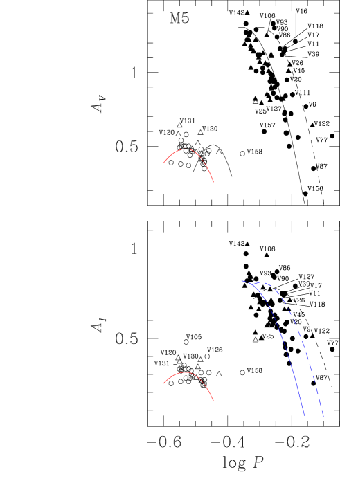
Fig. 6 : The log P vs. amplitude plane for the $V$ and $I$ amplitudes of the RRL in M5. Filled and open symbols represent RRab and RRc stars respectively. Triangles are used for stars with Blazhko modulations. In the top panel the continuous and segmented lines are the loci found by Cacciari et al. (2005) for unevolved and evolved stars, respectively, in the OoI cluster M3. In the bottom panel the black segmented locus was found by Arellano Ferro et al. (2011, 2013) for the OoII clusters NGC 5024 and NGC 6333. The blue loci are from Kunder et al. (2013) for the OoI cluster NGC 2808. The red parabolas were calculated by Arellano Ferro et al. (2015b) for a sample of RRc stars in five OoI clusters. The black parabola was found by Kunder et al. (2013b) for 14 OoII clusters.

Several features can be highlighted from the distribution of RRL in the HB from its expanded version in the bottom panel of Fig. 3, in combination with the Bailey diagram of Fig. 6 and the period-colour diagram displayed in Fig. 7, very useful for the task of interpreting the distribution of RRL stars in the instability strip. In this last diagram, the period $\log P^{\prime}=\log P+0.336(<V>-15.021)$, where 15.021 mag is the average $<V>$ for all the stable RRL, is plotted as a function of $<V>-<I>$. The use of $P^{\prime}$ significantly reduces the scatter in the diagram (van Albada & Baker 1971; Bingham et al. 1984).

Stable RRab and RRc stars as well as those exhibiting Blazhko modulations have been distinguished in these three figures. Let us note first that all RRab stars falling in the evolved sequence of the top panel of Fig. 6 have been plotted with red filled circles and red labels in the bottom panel of Fig.3, and they are $bonafide$ the brightest stars, as expected for stars in an advanced evolutionary state towards the AGB. However a higher luminosity can be attained by non-evolutionary means, like the presence of an unseen companion or the existence of atmospheric enrichment of helium due to extra mixing at the RGB stage (Sweigart 1997). Let us note the labelled outlier stars in Fig. 7 (V93, V107, V108, V118, V119, V122, V125, V158) (other peculiar outliers V25, V104 and V142 are discussed below in section A). These stars are labelled in the bottom panel of Fig. 3 in black. These stars have too short a period for their colour which implies that they have larger gravity and should be of lower luminosity. If in spite of this they happen to be among the most luminous stars in the IS, then they are good candidates to have a companion. This seems to be the case of V107, V122 and V158. Similar cases were identified by Cacciari et al. (2005) among the RRL in M3 (V48, V58, and V146) and by Arellano Ferro et al. (2015b) in NGC 6229 (V14, V31, V54 and V55). Thus, these stars with shorter periods compared to others of similar colour, could have enhanced helium in their atmospheres or have become luminous due to the presence of an unseen companion. The remainder of the stars with red symbols might be truly evolved stars. Unfortunately none of this was included in the secular period change analysis of Szeidl et al. (2011) perhaps because most of them were only discovered after 1987 and the time-base of existing data is not long enough.

4.2 The RRab-RRc segregation and the Oosterhoff type

It has been noted and discussed in several of our recent papers that some clusters show a neat splitting in the distribution of stable RRab and RRc stars in the CMD with the border at $(V-I)_{0}\sim 0.45-0.46$. In Fig. 3 the corresponding border lines for NGC 6229, NGC 5024 and NGC 4590 duly reddened are indicated by vertical black dashed lines. A detailed discussion of this fact has been given by Arellano Ferro et al. (2015b) (their section 5). In brief, a clear RRab-RRc splitting is distinguished in the OoII clusters NGC 288, NGC 1904, NGC 5024, NGC 5053, NGC 5466, NGC 6333 and NGC 7099, all with rather blue HBs ($\cal L>$ 0.4). It is also observed in the OoII cluster NGC 4590 which has a red HB ($\cal L$=0.17)(see CMD in Fig. 11 of Kains et al. 2015). Among OoI clusters, NGC 3201 does not present the splitting (Arellano Ferro et al. 2014) while NGC 6229 does, very clearly (Arellano Ferro et al. 2015b).

In Fig. 8 we have plotted the Lee-Zinn parameter $\cal L$ as a function of [Fe/H]_ZW taken mostly from Table 2 in Catelan (2009). The OoII clusters all show blue tails, except NGC 4590. The more metallic OoI clusters may have both blue and red HBs and display a large dispersion. Those clusters for which we have explored the RR Lyrae distribution are plotted with filled symbols while empty symbols are used otherwise. Three OoI clusters are also labelled; despite their closeness in the plot the only one with a clear RRab-RRc segregation is NGC 6229, while NGC 3201, and now M5 (see Fig. 3), show both Blazhko and stable RRab stars well distributed all across the IS, in the either-or region, i.e. to the blue of the first-overtone red border. It should be noted however that in all cases stable RRc stars are well confined to the blue of the first-overtone red border as expected. In passing let us mention that this is yet another important difference between M5 and ”its twin” NGC 6229.

It is true that we have explored only three OoI clusters and that an analysis of a larger number of both types of Oosterhoff clusters is desirable; however, we might preliminarily conclude that blue-tailed OoII clusters seem to have their RRab and RRc stars systematically well segregated around the red border of the first-overtone instability strip. However, OoI clusters may or may not have this property.

Fig. 7 : Period-colour diagram of stable RRL stars. Filled circles are used for RRab stars and empty circles for RRc stars. Triangles are used for stars with Blazhko modulations. The periods of the RRc stars were fundamentalized by adding 0.128 to log $P$. The reduced period $P^{\prime}$ is defined as $\log P^{\prime}=\log P+0.336(<V>-15.021)$.

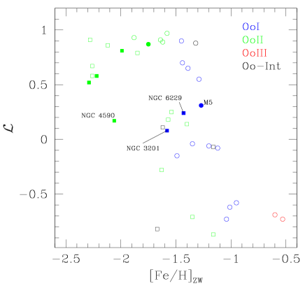
Fig. 8 : Distribution of HB structure parametrized by the Lee-Zinn parameter $\cal L$ as a function of [Fe/H]_ZW for Galactic GCs of different Oosterhoff types, according to the legend, with data taken from Catelan (2009). Inner and outer halo clusters are represented by circles and squares respectivelly

.

The distribution of RRL on the HB may be explained by the arguments of Caputo et al. (1978) which involve the occurrence of a hysteresis mechanism (van Albada & Baker 1973) for stars crossing the IS. According to this mechanism the stars in the ”either-or” region can retain the mode they were pulsating in before entering the region, which depends on whether the star is coming from the blue side as an RRc or from the red side as an RRab. Caputo et al. (1978) also suggest that the original mode in which a RRL is pulsating depends on the location of the starting point at the Zero Age Horizontal Branch (ZAHB), which in turn depends on the mass and the chemical composition of the star; they used these ideas to explain the existence of the two Oosterhoff groups as follows; 1) the ZAHB point is in the fundamental zone, leading to an assortment of RRc and RRab in the ”either-or” region and a lower value of the average period for both RRc and RRab and a lower proportion of RRc stars, hence an OoI cluster, and 2) the ZAHB point is bluer than the fundamental zone, in the ”either-or” or in the first overtone regions, then the ”either-or” region is populated exclusively by RRc stars and the RRab stars are to be found only in the fundamental region, producing larger averages of periods and a higher proportion of RRc and hence an OoII type cluster.

The above scenario explains well the clean segregation of RRc and RRab seen in the OoII clusters, or the definitive lack of segregation in OoI clusters like NGC 3201 or M5, but, as commented by Arellano Ferro et al. (2015b), the clean segregation observed in the OoI cluster NGC 6229 is at odds with the above picture.

Furthermore, RRab-RRc segregation in OoII clusters is also favoured by the arguments of Pritzl et al. (2002) that in clusters with blue HBs, i.e. large values of $\cal L$, stars with masses below a critical mass on the ZAHB to the blue of the IS, evolve redwards and spend sufficient time to contribute to the population of RRL. Thus, clusters with a blue HB morphology are OoII, with redwards evolution, which in turn favours the segregation between RRc and RRab on the IS which, in passing, should at least statistically display increasing secular period variations. Unfortunately there are few clusters with a large enough number of RRL with secularly changing periods that have been studied; e.g. the OoII clusters Omega Cen (Martin 1938) and M15 (Silbermann & Smith 1995) and the OoI clusters M3 (Corwin & Carney 2001) and M5 (Szeidl et al. 2011); in all these clusters only a small surplus, and probably not statistically significant, of RRL are reported as having increasing periods.

Growing evidence of the existence of multiple stellar populations in GCs (see for instance Jang & Lee (2015) and the references therein) invites us to consider whether this is connected with the observed RRab-RRc splitting discussed above. According to Jang & Lee (2015), in inner-halo GCs the time elapsed between the first stellar generation (G1) and a helium ($Y$) and CNO enhanced second generation (G2) is $\sim$ 0.5 Gyr while in the outer-halo GC’s, G1 has been delayed by $\sim$ 0.8 Gyr and the time between G1 and G2 has been longer, $\sim$ 1.4 Gyr. They have demonstrated that for metallicities [Fe/H]$\sim-1.5$, in outer GC’s the IS is mostly (but not exclusively) populated by G1 while the $Y$- and CNO-enhanced G2 RR Lyrae stars must be more luminous (see their figure 7) with an average $<P_{ab}>=0.552$d, which agrees very well with the observed $<P_{ab}>=0.553$d in M5. For inner GC’s of similar metallicity the mix of G1 and G2 in the IS is likely more due to the shorter time between generations in which case $<P_{ab}>=0.607$d. For lower metallicity outer GC’s, [Fe/H]$\sim-2.0$, the IS is populated basically by G2 stars. We shall recall that for a $Y$- and CNO-enhanced G2, the masses on the ZAHB are shifted towards lower temperatures (Jang et al. 2014, their figure 3), hence displacing the first overtone red-edge (FRE) to the red (Bono Caputo & Marconi 1995). More than one generation sharing the IS will have different FRE boundaries contributing to a mix of RRc and RRab stars.

What effect the above scenario might have on the presence or not of the RRab-RRc splitting is not clear at present as several factors seem to play a role; the overall metallicity, the presence of more than one generation in the IS and the time elapsed between generations. We could add to this the possible presence of pre-ZAHB RR Lyrae stars (Silva Aguirre et al. 2008). Clearly more investigation of a larger sample of GC’s is necessary to confront the observations with theoretical predictions. We speculate that in outer-halo OoII clusters the larger time difference between generations favours the existence of an RRab-RRc splitting as we have generally observed.

5 Distance and metallicity of M5 from its variable stars

The distance to M5 can be estimated from our data using different approaches; firstly, from the weighted mean $M_{V}$, calculated for the RRab and RRc from the Fourier light curve decomposition (Table 5), which can be considered as independent estimates since they come from different empirical calibrations and zero points. Secondly, we can use the $I$-band RR Lyrae P-L relation derived by Catelan, Pritzl & Smith (2004). As a third approach we can use the three known SX Phe stars and their P-L relation. And finally a fourth approach is via the bolometric magnitude for stars at the tip of the RGB. Below we expand on these solutions.

Being M5 a nearby cluster, its reddening is small, we adopted $E(B-V)$=0.03 mag (Harris 1996). Given the mean $M_{V}$ for RRL in Table 5 we found a true distance modulus of $14.403\pm 0.067$ mag and $14.387\pm 0.094$ mag using 38 RRab and 24 RRc stars respectively, which correspond to the distances $7.6\pm 0.2$ and $7.5\pm 0.3$ kpc. The quoted uncertainties are the standard deviations of the corresponding means. The distance to M5 listed in the catalogue of Harris (1996) (2010 edition) is 7.5 kpc in good agreement with our calculations.

The $I$-band RR Lyrae P-L relation derived by Catelan, Pritzl & Smith (2004) is of the form:

$$M_{I}=0.471-1.132{\rm log}P+0.205{\rm log}Z,$$ (4)

with ${\rm log}Z=[M/H]-1.765$. We applied these equations to all 62 RRab and RRc stars in Table 5. The periods for the RRc stars were fundamentalized following the period ratio $P_{1}/P_{0}=0.7454$ in double mode stars (Catelan 2009). We found an average distance of 7.2$\pm$0.3 kpc.

An independent estimate of the distance can be obtained from the three SX Phe known in the cluster. Fig. 9 shows the P-L relationship of Cohen & Sarajedini (2012);

$$M_{V}=-(1.640\pm 0.110)-(3.389\pm 0.090){\rm log}P_{f}$$ (5)

positioned for the RRL mean distance. The first-overtone and second-overtone lines were positioned adopting the frequency ratios $F/1O$= 0.783 and $F/2O$ = 0.571 (see Santolamazza et al. 2001 or Jeon et al. 2003; Poretti et al. 2005). It seems clear from the plot that V164 is a fundamental pulsator while V160 and V170 pulsate in the first-overtone. Then, adopting eq. 5 we find an average true distance modulus of $14.428\pm 0.150$ or a distance of $7.7\pm 0.4$ kpc. The uncertainty was calculated from calibration errors neglecting the uncertainty in the period.

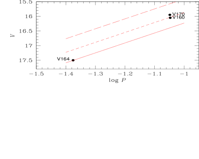
Fig. 9 : M5 SX phe stars in the Period-Luminosity plane. The lines are the P-L relationship for the SX Phe fundamental mode(continuous) of Cohen & Sarajedini (2012), first-overtone (short segmented) and second-overtone (long segmented).

Yet another approach to the cluster distance determination is by using the tip of the RGB. This method was developed for estimating distances to nearby galaxies (Lee, Freedman & Madore, 1993). One possibility is to use the specific calibration of the bolometric magnitude of the tip of the RGB, of M5 by Viaux et al. (2013) under the arguments that the neutrino magnetic dipole moment enhances the plasma decay process, postpones helium ignition in low-mass stars, and therefore extends the red giant branch (RGB) in GCs. These authors came to the conclusion that in M5 $M_{bol}^{tip}$= -4.17 $\pm$ 0.13 mag and we adopted that value. As in Arellano Ferro et al. (2015b) for the case of NGC 6229, we found that the method is extremely sensitive to the star selection. Reasonable results are found for the stars nearest to the tip of the RGB, i.e. the reddest and brightest in this region of the CMD. We restricted our calculation to the two brightest RGB stars in our sample V50 and V174. According to Viaux et al. (2013), the TRGB is between 0.05 and 0.16 mag brighter than the brightest stars on the RGB. The fact that V50 and V174 may not be the brightest stars on the RGB implies that their magntiudes would have to be corrected to bring them to the TRGB by at least the above quantities; the larger the correction the smaller the resulting distance. We applied a correction between 0.05 and 0.16 mag to V50 and V174 and found a mean distance of between 7.5 and 7.2 kpc respectively.

The above independent estimations of the cluster distance are, within their uncertainties, satisfactorily in agreement. However, given the sensitivity of the SX Phe P-L and the TRGB approaches to the number of stars involved as well as to the sample selection, we believe that the distance determinations from the RRL stars, which deal with much larger samples and carefully calibrated zero points of the luminosity scale are the best achieved.

For the metallicity, the overall average value from the RRL is [Fe/H]${}_{\rm UVES}=-1.36\pm 0.16$ or [Fe/H]${}_{\rm ZW}=-1.47\pm 0.14$ found from the Fourier decomposition of the light curves of 38 RRab and 24 RRc. These values can be compared with previous values in the literature: [Fe/H]${}_{\rm ZW}=-1.29$ (Harris 1996); [Fe/H]${}_{\rm ZW}=-1.23$ (Kaluzny et al. 2000) from an independent Fourier decomposition analysis; [Fe/H]${}_{\rm ZW}=-1.44$ (Zinn 1985); [Fe/H]${}_{\rm UVES}=-1.11\pm 0.03$ (Carretta et al. 2009)

5.1 On the age of M5

The age of M5 has been discussed in numerous works. We have not attempted an independent estimation. The age of M5 was determined by Jimenez & Padoan (1998) via its luminosity function and they found an age of $10.6\pm 0.8$ Gyr assuming [$\alpha$/Fe]=+0.4. Two more recent determinations of the age of M5 are by Dotter et al. (2010) using relative ages from isochrone fitting, and by VandenBerg et al. (2013) using an improved calibration of the ”vertical method” or the magnitude difference between the turn off point and the HB; these authors find 12.25$\pm$0.75 Gyr and 11.50$\pm$0.25 Gyr respectively. Thus, in the CMD of Fig. 3 we have overlayed the corresponding isochrones for 12.0 Gyr from the Victoria-Regina evolutionary models (VandenBerg et al. 2014) and for the metallicities [Fe/H]=$-1.42$ (red) and [Fe/H]=$-1.31$ (blue) and [$\alpha$/Fe]=+0.4, shifted for the average apparent distance modulus $\mu$=14.395 mag found from the RRab and RRc stars, and $E(V-I)=1.616E(B-V)=0.048$.

The isochrones for these two metallicities are very similar except perhaps at the tip of the RGB where the isochrone for the more metal-rich composition gets less luminous. However, if shifts are applied to these isochrones within the uncertainty of the distance modulus and reddening, $\sim 0.1$ mag, the two cases are indistinguishable. We can stress then that our CMD is consistent with the metallicity and distance derived in this paper and an age of $12.0\pm 1.0$ Gyr found in the above papers for M5.

6 Summary and discussion

The Fourier decomposition of the light curves of stable RRL, and the calibrations and zero points available in the recent literature allowed us to determine the mean metallicity and distance to M5 as [Fe/H]${}_{\rm UVES}=-1.34\pm 0.11$ and $-1.39\pm 0.12$ and $7.6\pm 0.2$ kpc and $7.5\pm 0.3$ kpc, from the RRab and RRc stars respectively. Also individual values of radius and mass are provided. The employment of the $I-band$ RR Lyrae P-L relation leads to a distance of 7.2$\pm$0.3 kpc. The distance to the cluster was also estimated from two independent methods; the P-L relation of SX Phe and the luminosity at the tip of the RGB finding 7.7$\pm$0.4 kpc and 7.5$\pm$0.1 kpc respectively. However we have shown that in the case of M5 the accuracy of these two alternative methods does not compete with the accuracy attained with the RR Lyraes and the Fourier light curve decomposition.

A group of 16 evolved stars have been identified from their distribution in the amplitude-period plane. Evolved stars should be moving to the red in the CMD, hence their periods should be increasing. From the period change study of Szeidl et al. (2011) and our own period change analysis, which will be published elsewhere, we can see that some stars have increasing periods (V11, V16, V39, V45, V77, V87 and V90) and some have clearly decreasing periods (V9, V12 and V17), which might be unexpected in truly evolved stars. However it is understood now that stochastic processes may produce both positive, negative or irregular period variation, e.g. mixing events in the core of a star at the HB (Sweigart & Renzini 1979) or, as suggested more recently by Silva Aguirre et al. (2008), period decreases can occur in pre-ZAHB RR Lyrae stars on their final approach to the ZAHB. In the bottom panel of Fig. 3 we have drawn a small line segment from the corresponding circles, to the right or left to indicate period increase or decrease respectively. The remainder of the evolved stars were not found to be undergoing secular period variations in our analysis. From their position on the CMD, their long period value and large period change rate, we conclude that V77 and V87 are truly advanced in their evolution towards the AGB.

For the most luminous stars in the IS (V107, V122 and V158) we argue that they are not truly evolved stars but owe their overluminosity to a helium enhanced atmosphere or to the presence of an unseen companion.

We note that in the HB instability strip of M5, RRab stars share the either-or region with RRc stars, like in the case of the OoI cluster NGC 3201, but in contrast with NGC 6229, a cluster presumably nearly a twin of M5, where the RRab-RRc splitting is noticeable. We also highlight the fact that the RRab-RRc splitting is a common feature in OoII clusters with a blue tail.

Our CCD $VI$ time-series, spanning a little more than two years, allowed us to detect amplitude and phase modulations in 14 RRab and 9 RRc stars not previously reported as having the Blazhko effect. These new findings account for incidence rates of at least 38% and 26% of the RRab and RRc respectively showing the Blazhko effect in M5. This comes as a natural result since in the last few years the detection of Blazhko variables in GCs has been increasing, most likely due to the improvement in the quality of the CCD observations and reduction techniques. Take for example the cluster NGC 5024 with the largest known population of Blazhko variables with 66% and 37% of RRab and RRc respectively (Arellano Ferro et al. 2012).

Finally, it is well known from key studies in the past (e.g. Oosterhoff 1941, Szeidl et al. 2011) that a large fraction of the RRL population of M5 is undergoing secular period variations. Our present data add up to 20 years to the time-base of available data for M5 and a re-analysis of the period change rates is deferred to a forthcoming paper.

Appendix A Comments on individual stars and the Blazhko variables

In this section we comment on the light curves, variable types and nature of some interesting or peculiar variables in Table 3 and Figs. 4 and 5. We put some emphasis on the amplitude and phase modulations of the Blazhko type in specific stars. In all the stars labelled ’$Bl$’ in Table 3 the amplitude variations are neatly distinguished in the light curves in Figs. 4 and 5 in both the $V$ and $I$ filters.

V25, V36, V53, V74, V102, V108, V140 and V159. All these stars were found by Arellano Ferro et al. (2015a) to be misidentified in the literature. In that paper the identifications have been discussed and corrected and a detailed identification chart is given.

V14. In the CVSGC (2014 update) it is noted as an unconfirmed variable, probably after Evstigneeva et al. (1995). However the star is clearly variable in the study of Kaluzny et al. (2000) and in the present work. It displays some amplitude modulation already noted by Kaluzny et al. (2000).

V18. It displays a tremendous amplitude variation from 0.617 mag in 2012 to 1.218 mag in 2013 and 2014. The observations on January 23, 2013 are already consistent with the large amplitude, meaning that the star underwent the amplitude change between May 2012 and January 2013. The photographic light curve from 1934 from Oosterhoff (1941), although a bit scattered, shows an amplitude of 0.76 mag and while not directly comparable with our $V$ or $I$ light curve amplitudes we mention that Oosterhoff himsef noted considerable light curve variations and suggested to classifiy it as an irregular variable. The data from 1997 of Kaluzny et al. (2000) show an amplitude of 1.27 mag and a mild suggestion of the Blazhko effect. The repetitivity of our light curves from February to May in 2012 at the low amplitude and again during 2013-2014 at the large amplitude, suggests that the star remains with a constant amplitude before it goes through the amplitude variation episodes: it is therefore a very strong Blazhko modulator with a rather long period. According to Szeidl et al. (2011) the Blazhko period is longer than 500d.

V25. This star is heavily blended with a nearby star which explains the relatively noisy light curve in Fig. 4. It has been discussed and clearly identified by Arellano Ferro et al. (2015a).

V27. Despite its relative isolation it shows a very peculiar light curve. We have not been able to identify more than one period. Thus the observed amplitude and phase modulations must be due to the Blazhko effect. We adopted the period of Szeidl et al. (2011) that phases the light curve best. They did not find secular period changes for this star. The Blazhko modulations are very prominent.

V28. Similar to V18, this star shows a very pronounced amplitude modulation from 1.120 mag to 0.653 mag with much different time distributions than V18. The amplitudes in the light curves of Oosterhoff (1941) and Kaluzny et al. (2000) are in between the above two extremes.

V42, V84. These two W Virginis (CW) stars are shown in the CMD of Fig. 3 and their light curves are displayed in Fig. 10. The data are included in the electronic Table 2. Their periods are listed in Table 3. For V42 the period 25.735d given in the CVSGC phases our data correctly. For V84 the period 53.95d in the CVSGC does not phase our data properly but we found that about half of it, 26.49d, produces a nice light curve.

Fig. 10 : Light variations of the CW stars V42 and V84 phased with the ephemerides given in Table 3.

V50,V171-V181. A discussion and the light curves of all these semi-regular late-type (SRA) variables can be found in the paper by Arellano Ferro et al. (2015a).

V77. This is the RRab with the largest period in M5 (0.845158d). It has a low amplitude and a peculiar shape of the light curve with a roundish maximum. In the amplitude-period diagram (Fig. 6) the star falls in the extreme right of the diagram, much beyond the evolved stars sequence. In the CMD (bottom of Fig. 3) it is one of the brightest stars. The star is undergoing a secular period increase with a rate among the largest in M5 (Szeidl et al. 2011). All these properties are consistent with the star being in an advanced evolutionary state towards the AGB.

V78. This star has the shortest period among the known RRL stars in M5 (0.264820d). Kaluzny et al. (2000) have argued that it may be a second overtone pulsator (RRe) and noted the slight asymmetry of the light curve. We point out that while the asymmetry is there, it appears as prominent as in the other RRc stars with longer periods (e.g. V15, V55, V60 etc.). In fact, an inspection of the light curves of the RRc stars in Fig. 5 reveals that a slight asymmetry is present in most of them, so this seems to be more the rule than the exception in this cluster. However, following Catelan’s (2004) practice, we have checked the log P - $<I>$ plane and confirmed that, after fundamentalizing the period of V78 assuming that it is a second-overtone pulsator, the star falls in the natural extension to short period of the RRab distribution. This seem to support the idea that V78 is a RRe.

V87. Like V77, this star has a long period and a small amplitude and it is also an evolved star with the corresponding large period increase rate (Szeidl et al. 2011).

V101. A discussion of our data of this cataclysmic variable of the U Gem type and its light curve is given by Arellano Ferro et al. (2015a).

V104. It has been noticed by several authors that the light curve of this peculiar star shows very prominent amplitude and phase modulations. It has been suggested to be a double mode star (Reid 1996) and a semi-detached binary (Drissen & Shara 1998). Its rather long period for an RRc star and its position among RRab stars on the log P - $<I>$ plane make it more likely to be an RRab star. We used period04 to search for traces of double mode activity but found no significant secondary frequencies. Our light curve is very peculiar indeed and shows multiple RR Lyrae-like curves, all well phased with a period of 0.486748, with phase and mean brightness displacements. It is probably an RRab in a binary system, unfortunatelly we could only estimate five times of maximum on our data and two in the light curve of Drissen & Shara (1998) and thus, with the handful of times of maximum the corresponding O-C diagram does not shed clear signs of duplicity.

V121. This star is close to the center of the cluster but it is not blended with another star of similar magnitude or brighter. Despite this, it shows large modulations in phase and amplitude probably due to the presence of Blazhko effect. The light curves in Caputo el al. (1999) and Drissen & Shara (1998) look stable but their time-base are very short.

V127. This star is very close to another of similar brightness. It is identified in the discovering paper (Kravtsov 1988) and we confirm that the variable is the NW of the pair (see Fig. 12). In the paper by Olech et al. (1999) its light curve appears as that of a small amplitude RRc-like with a period 0.544965d. However our period 0.540366d produces a clear RRab light curve with amplitude apparently diminished due to flux contamination by the neighbour. On the Bailey diagram (Fig. 6) the star clearly sits among the RRab stars. It also shows amplitude modulations.

V155. A light curve of this W Ursae Majoris-type eclipsing binary (EW) is presented and discussed in the paper by Arellano Ferro et. al. (2015a).

V156. The variability of this star and a nice looking RRab light curve were reported by Drissen & Shara (1998) from their high resolution images of the Hubble Space Telescope (HST), and they labelled it as V15. The star identified by these authors is strongly blended in our images and we were not able to either calculate a period at confidence or recover a RRL-like light curve, hence it was not included in Fig. 4. In Fig. 11 we show the nightly light variations and note the changes of the maximum brightness, inviting the suggestion of Blazhko modulations. Caputo et al. (1999) offered an alternative identification and named the star V156, however the light curve of that star does not show variations in our collection.

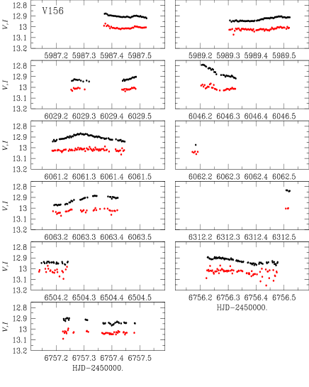
Fig. 11 : Light variations of the RRab star V156. Black and red circles are the $V$ and $I$ magnitudes, respectively. The $I$ magnitudes have been arbitrarily shifted to accommodate them in the same box, so that the variations in both filters can be appreciated.

V157. The light curve of this star has an anomalously low amplitude, likely due to blending in our images with a close bright star. Its position in the CMD (Fig. 3) and Bailey diagram (Fig. 6) is therefore peculiar.

V158. It is noted in the CVSGC as ”RRc?” Indeed its period 0.442627d is rather long for an RRc, however, its light curve is a little asymmetric and resembles that of the other RRc stars in the cluster. In the Bailey’s diagram (Fig. 6), the star falls halfway between the RRc and the RRab distributions. We have labelled it as RRc.

V159. An eclipse for this eclipsing binary (E) was detected in our data. The light curve is presented and discussed in the paper by Arellano Ferro et al. (2015a).

V170. The phased light curve for this SX Phe stars is given by Arellano Ferro et al. (2015a).

Interfering close pairs. We have identified a few close pairs of variable stars in our images that, depending on the seeing conditions may or may not have contaminated each other’s light curves. We list them below and briefly discuss them.

V84-V93 The RRab V93 is 12.5 pixels or 3.7 arcsec from the bright CW V84 which has produced the noisy appearance of the light curve in Fig. 3.

V109-V142. These two RRab stars are separated by only 4.0 pixels or 1.2 arcsec in our images and hence the interference of each other’s light curves which is evident as noise (see Table 1). The light curve of V142 shows very prominent phase and amplitude modulations. The variability was discovered by Brocato, Castellani & Ripepi (1996) but the light curve was not made available. Partial light curves were displayed by Caputo et al. (1999) and Drissen & Shara (1998) where the variations are clear but no modulation was detected, most likely due to the limited time-base of these data sets.

V112-V113. The separation of these stars is 7.4 pixels or 2.2 arcsec which means that in nights of poorer seeing their light curves are contaminated by the light of the neighbour producing noisier light curves.

V130-V131. These stars are separated by 8.4 pixels or 2.5 arcsec, i.e. ocassionally, on nights of poorer seeing there is mutual light contamination. Scatter in the light curve of V130 was noted by Kaluzny et al. (2000) but their search for a secondary frequency was futile. Our light curve shows clear amplitude modulations which could be attributed to the Blazhko effect. V131 is not included by Kaluzny et al. Both stars included by Caputo et al. (1999) show no amplitude modulations but their light curves are sparse. In our data V131 also shows mild amplitude modulations. It is possible that the observed amplitude modulations are due, at least partially, to the light contamination from the neighbour.

RRab stars with Blazhko modulations. A systematic and thorough analysis of 50 RRab stars in M5 was conducted by Jurcsik et al. (2011) in search of Blazhko-type variability and its characterization, using a collection of photometry of M5 covering nearly 100 years. They identified 20 Blazhko stars among the RRab population and calculated the modulation periods (their Table 1). The modulation periods range mostly between 40 and 600 days, with the exception of V72 for which the modulation is about 1200 days. The time-base of our data is 770 days (see Table 1). This means that based only on our observations we should be able to detect the modulations in all those variables, provided that the modulations are strong enough and the photometry is of good quality. Of the 20 stars found by Jurcsik et al. (2011) four (V2, V29, V58 and V72) are not in the FoV of our images. The remaining 16 stars are labelled ’$Bl^{b}$’ in Table 3, however V5, V30 and V38, look rather stable in our light curves, thus we would have been unable to identify these as Blazhko variables based exclusively on our data. We find it difficult to judge the real Blazhko nature of these three stars. We note first that the Blazhko modulations reported by Jurcsik et al. (2011) are in all cases very mild and that for V5 and V38 the Blazhko classification relies on a comparison between the data from Reid (1996), whose light curves are a bit scattered, and the data from Kaluzny et al. (1999; 2000) separated by 5 years; both stars are in crowded fields and Kaluzny et al. 2000 has pointed out that neighbours at 5-10 arcsec affect some of the photometric data. For the more isolated star V30 the comparison was between the data of Storm et al. (1991) and Kaluzny et al. (1999; 2000) separated by 10 years, reduced and transformed to the standard system by different approaches. While these details may contribute to apparent amplitude differences, it is also possible that our data time-base is not long enough for the detection of a long-period modulation. For the other 13 stars the modulations are also evident in our data.

Besides the above mentioned stars, we have also been able to detect amplitude-phase modulations in the light curves of another 14 RRab stars, some of which are subtle but visible, hence probably undetectable in old photographic data. These 14 newly identified Blazhko RRab stars are labelled ’$Bl$’ in Table 3. This makes a total of 30 Blazhko stars in M5 in a sample of 79 RRab stars, i.e. an occurrence rate of at least 38%.

RRc stars with Blazhko modulations. No Blazkho RRc variables were reported by Jurcsik et al. (2011). However, the modulations are clearly visible in 9 stars of the 34 in our sample; V35, V40, V44, V53, V55, V99, V120, V130 and V131. This makes an incidence rate of at least 26% for RRc Blazhko variables in M5.

RRc stars with prominent bump near maximum. The presence of bumps near the maximum light in RRc stars is clear in V31, V35, V57, V60, V62, V95, V100, V105, V108, V113, V116, V130 and V133. Bumps were noted before by Kaluzny et al. (2000) in V31, V35, V57 and V62 and highlighted that bumps do not occur for stars with periods above 0.28-0.30 d, which is true also for our extended list of ”bumpy” stars with the exception of V108 and V130 with P$\sim$0.328, although we may concede that the bump in these cases is rather mild. Kaluzny et al. (2000) venture the possibility that the bump is associated with some sort of interaction between the first and second overtones. The bump was actually reproduced in the RRc star U Com by hydrodynamical models constraining the metallicity and calibrating the adopted turbulent convection model. The bump was found to be sensitive to the parameters governing the coupling between convection and pulsation (Bono, Castellani & Marconi 2000).

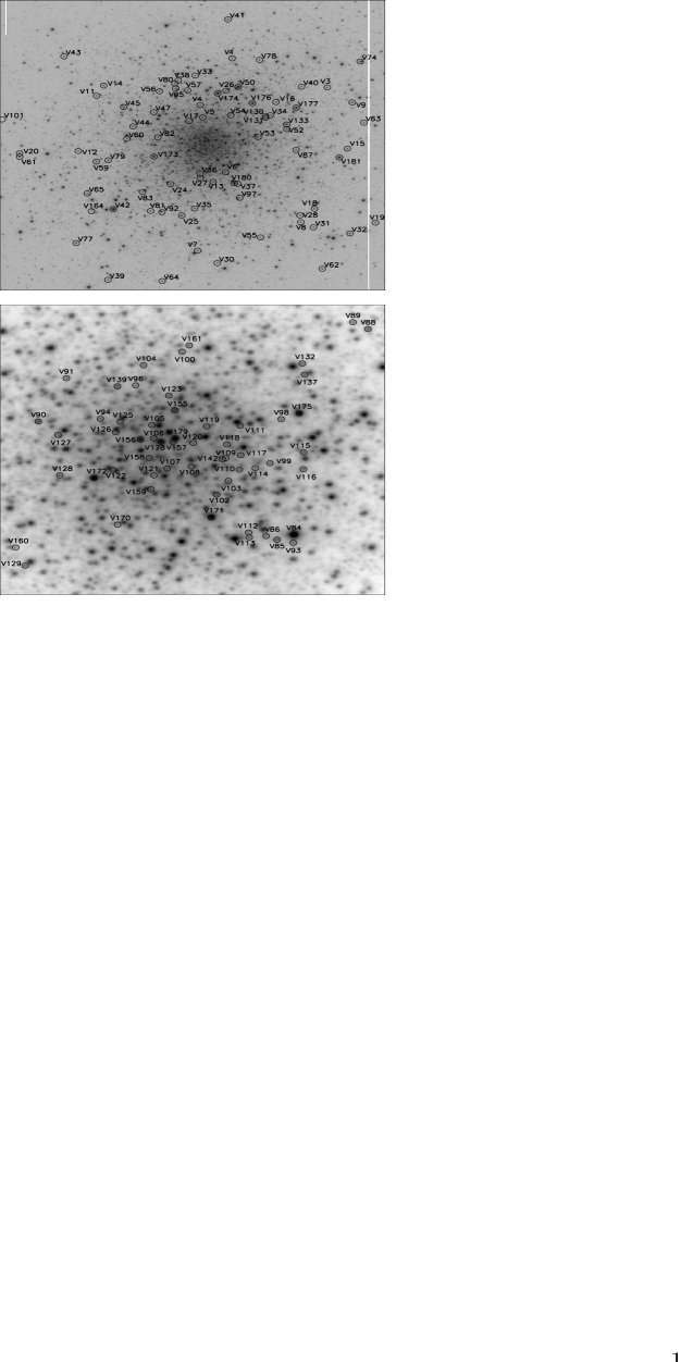
Fig. 12 : Finding charts constructed from our $V$ reference image; north is up and east is to the right. The cluster image at the top is 8.8$\times$8.8 arcmin². The core image at the bottom is 2.2$\times$2.2 arcmin². All of the variable stars listed in Table 3 are identified.

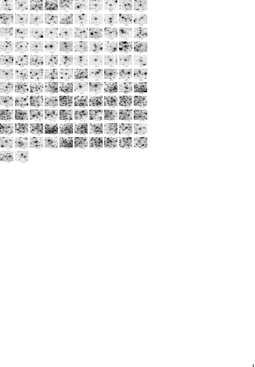
Fig. 13 : Individual star cut-outs for each star in Fig. 12. Images are of size 23.7$\times$23.7 arcsec². All of the stars listed in Table 3, except for those with cutouts already published in Arellano Ferro et al. (2015a), are shown.

References

- (1) Arellano Ferro, A., Ahumada, J. A., Calderón, J.H., Kains, N., 2014, RMAA, 50, 307
- (2) Arellano Ferro, A.; Bramich, D. M.; Figuera Jaimes, R.; Giridhar, Sunetra; Kuppuswamy, K., 2012, MNRAS, 420, 1333
- (3) Arellano Ferro, A., Bramich, D. M., Giridhar, S., Luna, A., Muneer, S., 2015a, IBVS 6137
- (4) Arellano Ferro, A., Mancera Piña, P. E., Bramich, D. M., Giridhar, s., Ahumada, J.H., Kains, N., K. Kuppuswamy, 2015b, MNRAS, 452, 727
- (5) Arellano Ferro, A., Bramich, D. M., Figuera Jaimes, R., et al., 2013, MNRAS, 434, 1220
- (6) Arellano Ferro, A., Figuera Jaimes, R., Giridhar, Sunetra, Bramich, D. M., Hernández Santisteban, J. V., Kuppuswamy, K., 2011, MNRAS, 416, 2265
- (7) Barnard, E.E., 1898, AN, 147, 243
- (8) Bailey, S. I., 1902, ApJ, 10, 255
- (9) Bailey, S. I., Leland, E. F., 1899, ApJ, 10, 255
- (10) Bingham E. A., Cacciari C., Dickens R. F., Fusi Pecci F., 1984, MNRAS, 209, 765
- (11) Bono, G., Castellani, V., Marconi, M., 2000, ApJ, 532, L129
- (12) Bono, G., Caputo, F., Marconi, M., 1995, AJ, 110, 2365
- (13) Borissova, J., Catelan, M., Ferraro, F. R., Spassova, N., Buonanno, R., Iannicola, G., Richtler, T., Sweigart, A. V., 1999, A&A, 343, 813
- (14) Bramich D. M., 2008, MNRAS, 386, L77
- (15) Bramich, D. M., Bachelet, E., Alsubai, K. A., Mislis, D., Parley, N., 2015, A&A, 577, A108
- (16) Bramich D. M., Figuera Jaimes R., Giridhar S., Arellano Ferro A., 2011, MNRAS, 413, 1275
- Bramich & Freudling (2012) Bramich D. M., Freudling W., 2012, MNRAS, 424, 1584
- (18) Bramich D. M., Horne, K., Albrow, M. D., and 8 coauthors, 2013, MNRAS, 428, 2275
- (19) Brocato, E., Castellani, V., Ripepi, V., 1996, AJ, 111, 809
- Burke et al. (1970) Burke E.W., Rolland W.W., Boy W.R., 1970, JRASC, 64, 353
- Cacciari, Corwin & Carney (2005) Cacciari, C., Corwin, T. M., Carney, B. W., 2005, AJ, 129, 267
- (22) Caputo, F., Castellani, V., Marconi, M., Ripepi, V., 1999, MNRAS, 306, 815
- (23) Caputo F., Castellani V., Tornambé A., 1978, A&A, 67, 107
- Carreta (2009) Carretta, E., Bragaglia, A., Gratton, R., D’Orazi, V., Lucatello, S., 2009, A&A, 508, 695
- (25) Catelan M., 2004, in , ASP COnference Series; editors D.W. Kurtz & K.R. Pollard, 310, 113.
- (26) Catelan M., 2009, Ap&SS, 320, 261
- (27) Catelan, M., Pritzl, B. J., Smith, H. A., 2004, ApJS, 154, 633
- Cement (2001) Clement, C. M., Muzzin, A., Dufton, Q., Ponnampalam, T., Wang, J., Burford, J., Richardson, A., Rosebery, T., Rowe, J., Hogg, H. S., 2001, AJ, 122, 2587
- (29) Cohen, R. E., Sarajedini, A., 2012, MNRAS, 419, 342
- (30) Cudworth K.M., 1997, In: Humphreys R.M. (ed.) Proper Motions and Galactic Astronomy. ASP Conf. Ser.Vol. 127, ASP, San Francisco, 91
- (31) Cudworth K.M., Hanson, R., 1993, AJ, 105, 168
- (32) Corwin, T. M., Carney, B. W., 2001, AJ, 122, 3138
- (33) Dotter A. et al., 2010, ApJ, 708, 698
- Draper (2000) Draper P. W., 2000, in Manset N., Veillet C., Crabtree D., eds. ASP Conf. Ser. Vol. 216, Astronomical Data Analysis Software and Systems IX. Astron. Soc. Pac., San Francisco, p. 615
- (35) Drissen, L., Shara, M. M., 1998, AJ, 115, 725
- Dworetsky (1983) Dworetsky M. M., 1983, MNRAS, 203, 917
- (37) Evstigneeva, N. M., Shokin, Yu. A., Samus, N. N., Tsevetkova, T. M., 1995, Sov. Astron. Let., 21, 451
- Harris (1996) Harris, W. E., 1996, AJ, 112, 1487
- Honeycutt (1992) Honeycutt, R. K., 1992, PASP, 104, 435
- (40) Jang, S., Lee, Y-W., 2015, ApJS, 218, 31
- (41) Jang, S., Lee, Y-W., Joo, S-J., Na, CCh., 2014, MNRAS, 4433, L15
- (42) Jeon Y.-B., Lee M. G., Kim S.-L., Lee H., 2003, AJ, 125, 3165
- Jimenez (1997) Jimenez, R, Padoan, P., 1998, ApJ, 498, 704
- Jurcsik (1998) Jurcsik, J., 1998, A&A, 333, 571
- JurKov (1996) Jurcsik, J., Kovács G., 1996, A&A, 312, 111
- (46) Jurcsik, J., Szeidl, B., Clement, C., Hurta, Zs., Lovas, M., 2011, MNRAS, 411, 1763
- (47) Kadla, Z. I., Gerashchenko, A. N., Yablokova, N. V., Irkaev, B.N., 1987, Ast. Tsirk., 1502, 7
- (48) Kains, N. et al. 2015, A&A, 578, A128
- (49) Kaluzny, J., Thompson, I. B., Krzeminski, W., Pych, W., 1999, A&A, 350, 469
- (50) Kaluzny, J., Olech, A. Thompson, I., Pych, W., Krzeminski, W., Schwarzenberg, A., 2000, A&AS, 143, 215
- (51) Kovács, G., 1998, MmSAI 69, 49
- (52) Kovács, G., Kanbur, S. M., 1998, MNRAS, 295, 834
- (53) Kovács, G., Walker, A. R., 2001, A&A 371, 579
- (54) Kravtsov, V.V., 1988, Astron. Tsirk. 1526, 6
- (55) Kravtsov, V. V., 1991, Sov. Astron. Let., 17, 455
- (56) Kunder A., Stetson P. B., Catelan M., Walker A. R., Amigo P., 2013a, AJ, 145, 33
- (57) Kunder A. et al., 2013b, AJ, 146, 119
- (58) Lee, M.G., Freedman, W., Madore, B.F., 1993, ApJ, 417, 553
- Lenz & Breger (2005) Lenz P., Breger M., 2005, Communications in Asteroseismology, 146, 53
- (60) Martin, W. Chr., 1938, Leiden Ann, 17B, 1
- (61) Morgan S., 2013, in Guzik J. A., ChaplinW. J., Handler G., Pigulski A., eds, Proc. IAU Symp. 301, Precision Asteroseismology. Cambridge Univ. Press, Cambridge, p. 461
- Morgan (2007) Morgan, S., Wahl, J. N., Wieckhorts, R. M., 2007, MNRAS, 374, 1421
- (63) Olech, A., Wozniak, P. R., Alard, C., Kaluzny, J., Thompson, I. B., 1999, MNRAS, 310, 759
- (64) Oosterhoff, P. Th., 1939, Observatory, 62, 104
- (65) Oosterhoff, P. Th., 1941, Leiden Ann., 17, Part 4
- Padmanabhan (2008) Padmanabhan, N., Schlegel, D.J., Finkbeiner, D. P. and 21 authors, 2008, ApJ, 674, 1217
- (67) Pickering, E.C., 1896a, A. N., 139, 137
- (68) Pickering, E.C., 1896b, A. N., 140, 285
- (69) Poretti E. et al., 2005, A&A, 440, 1097
- (70) Pritzl B. J., Armandroff T. E., Jacoby G. H., Da Costa G. S., 2002, AJ, 124, 1464
- (71) Rees, R. F., 1993, AJ, 106, 1524
- Regnault et al. (2009) Regnault N., Conley, A., Guy, J., and 13 authors, 2009, A&A, 506, 999
- (73) Reid, N., 1996, MNRAS, 278, 367
- (74) Sandquist, E. L., Bolte, M., Stetson, P. B., Hesser, J. E., 1996, ApJ, 470, 910
- (75) Santolamazza P., Marconi M., Bono G., Caputo F., Cassisi S., Gilliland R. L., 2001, ApJ, 554, 1124
- (76) Samus N.N., Durlevich O.V., Kazarovets E V., Kireeva N.N., Pastukhova E.N., Zharova A.V., et al., 2009, General Catalog ofVariable Stars
- (77) Scholz, R.-D., Odenkirchen, M., Hirte, S., Irwin, M. J., Borngen, F., Ziener, R., 1996, MNRAS, 278, 251
- (78) Silbermann, N. A., Smith, H. A., 1995, AJ, 109, 1119
- (79) Silva Aguirre, V., Catelan, M., Weiss, A., Valcarce, A.A.R., 2008, A&A, 489, 1201
- Stetson (2000) Stetson, P. B., 2000, PASP, 112, 925
- (81) Storm, J., Carney, B.W., Beck, J. A., 1991, PASP, 1033, 1264
- (82) Sweigart, A. V., 1997, ApJ, 474, L23
- (83) Sweigart, A.V., Renzini, A., 1979, A&A, 71, 66
- (84) Szeidl, B., Hurta, Zs., Jurcsick, J., Clement, C., Lovas, M., 2011, MNRAS, 411, 1744
- vanAlbada (1971) van Albada T. S., Baker N., 1971, ApJ, 169, 311
- vanAlbada (1973) van Albada, T.S., Baker, N., 1973, ApJ, 185, 447
- VandenBerg (2013) VandenBerg D. A., Brogaard K., Leaman R., Casagrande L., 2013, ApJ, 755, 134
- VandenBerg (2014) VandenBerg, D. A., Bergbusch, P. A., Ferguson, J. W., Edvardsson, B., 2014, ApJ, 794, 72
- (89) Viaux, N., Catelan, M., Stetson, P. B., Raffelt, G. G., Redondo, J., Valcarce, A. A. R.; Weiss, A., 2013, A&A, 558, A12
- (90) Yan, L., Reid, N., 1996, MNRAS, 279, 751
- Zacharias (2013) Zacharias, N., Finch, C. T., Girard, T. M., Henden, A., Bartlett, J. L., Monet, D. G., Zacharias, M. I., 2013, AJ, 145, 44
- Zinn (1985) Zinn, R., 1985, ApJ 293, 424
- Zinn & West (1984) Zinn, R., West, M. J., 1984, ApJS, 55, 45