An ALMA Search for Substructure, Fragmentation, and Hidden Protostars in Starless Cores in Chamaeleon I

Abstract

We present an Atacama Large Millimeter/submillimeter Array (ALMA) 106 GHz (Band 3) continuum survey of the complete population of dense cores in the Chamaeleon I molecular cloud. We detect a total of 24 continuum sources in 19 different target fields. All previously known Class 0 and Class I protostars in Chamaeleon I are detected, whereas all of the 56 starless cores in our sample are undetected. We show that the Spitzer+Herschel census of protostars in Chamaeleon I is complete, with the rate at which protostellar cores have been misclassified as starless cores calculated as $<$1/56, or $<$ 2%. We use synthetic observations to show that starless cores collapsing following the turbulent fragmentation scenario are detectable by our ALMA observations when their central densities exceed $\sim$10⁸ cm^-3, with the exact density dependent on the viewing geometry. Bonnor-Ebert spheres, on the other hand, remain undetected to central densities at least as high as $10^{10}$ cm^-3. Our starless core non-detections are used to infer that either the star formation rate is declining in Chamaeleon I and most of the starless cores are not collapsing, matching the findings of previous studies, or that the evolution of starless cores are more accurately described by models that develop less substructure than predicted by the turbulent fragmentation scenario, such as Bonnor-Ebert spheres. We outline future work necessary to distinguish between these two possibilities.

1. Introduction

Dense molecular cloud cores are the eventual birthplaces of stars (e.g., Beichman et al., 1986; Di Francesco et al., 2007). Sensitive (sub)millimeter bolometers with large instantaneous fields-of-view have enabled rapid mapping of entire molecular clouds, and as a result dense cores are often identified via their dust continuum emission (e.g., Motte et al., 1998; Shirley et al., 2000; Johnstone et al., 2000, 2001; Enoch et al., 2006, 2007; Sadavoy et al., 2010; Pattle et al., 2015; Salji et al., 2015; Könyves et al., 2015; Kirk et al., 2015). After identification, they are typically classified as protostellar or starless based on the presence or absence, respectively, of a young stellar object (YSO) detected in the infrared (e.g., Benson et al., 1984; Beichman et al., 1986; Myers et al., 1987; Jørgensen et al., 2008; Enoch et al., 2009) or a molecular outflow (e.g., Hatchell & Dunham, 2009; Chen et al., 2010). Some authors identify a subset of starless cores as “prestellar cores” if evidence exists that they are gravitationally bound or unstable (see Di Francesco et al., 2007; Ward-Thompson et al., 2007, for reviews of this subject). In this work, we use the term “starless core” to refer to any core not found to be associated with a protostar, where protostar refers to a YSO still embedded in and accreting from its parent dense core. We avoid the term “prestellar” altogether since we lack the data to evaluate whether each core is bound or unstable.

While existing (sub)millimeter observations have been extremely successful at finding cores, these relatively low angular resolution single-dish continuum surveys have been unable to determine the detailed physical structure of starless cores, especially the substructures indicative of fragmentation that will eventually form multiple protostellar systems. Additionally, infrared observations with the Spitzer Space Telescope (Spitzer; Werner et al., 2004) and Herschel Space Observatory (Herschel; Pilbratt et al., 2010) can miss the most deeply embedded and lowest luminosity protostars, leading to incorrect classification of some protostellar cores as starless.

1.1. Fragmentation and Substructure in Starless Cores

Approximately half of all protostars are found in multiple systems (Looney et al., 2000; Maury et al., 2010; Chen et al., 2013; Tobin et al., 2016). Additionally, both starless and protostellar cores are often found to have irregular morphologies on $\sim$1000 AU scales based on mid-infrared extinction studies (e.g., Stutz et al., 2009; Tobin et al., 2010), suggesting conditions favorable for fragmentation. Indeed, simulations including the effects of radiative feedback predict that “turbulent fragmentation” – the process by which turbulent fluctuations in a dense core become Jeans unstable and collapse faster than the background core (e.g., Fisher, 2004; Goodwin et al., 2004) – is the dominant mechanism responsible for forming multiple systems, and that the fragmentation begins in the starless core stage (Offner et al., 2010).

To date, only a few, isolated cases of substructure and fragmentation in starless cores have been identified (e.g., Kirk et al., 2009; Chen & Arce, 2010; Nakamura et al., 2012; Bourke et al., 2012; Lee et al., 2013; Friesen et al., 2014; Pineda et al., 2011a, 2015). On the other hand, the largest interferometric survey of starless cores presented to date, a CARMA (Combined Array for Research in Millimeter-wave Astronomy) 3 mm continuum survey of 12 cores in Perseus, found no evidence for substructure and fragmentation (Schnee et al., 2010, 2012). However, this CARMA survey was only sensitive to compact structures with masses above $\sim 0.1$ M_⊙, and synthetic observations of the Offner et al. (2010) turbulent fragmentation simulations have shown that CARMA likely lacked the sensitivity necessary to detect substructure and fragmentation (Offner et al., 2012; Mairs et al., 2014). These same synthetic observations have shown that the Atacama Large Millimeter/submillimeter Array (ALMA) is capable of detecting substructure and fragmentation in starless cores, particularly once it enters full science operations.

1.2. Accurate Classification of Cores

The first starless core observed by Spitzer in the Cores to Disks Legacy Survey (c2d; Evans et al., 2003, 2009), L1014, turned out to harbor a low luminosity, embedded protostar (Young et al., 2004). In a full search of the c2d dataset, Dunham et al. (2008) found that $\sim$20% of the “starless cores” in c2d contained similarly low-luminosity protostars and were thus misclassified. They further postulated the existence of an even lower luminosity population of protostars below the sensitivity limit of Spitzer, based on the observation that they continued to detect protostars all the way down to their sensitivity limit of 0.01 L_⊙ at $d=230$ pc. Such extremely faint protostars have started to be found in recent years, most through interferometer detections of outflows and/or compact continuum emission from cores classified as starless in Spitzer observations (e.g., Enoch et al., 2010; Chen et al., 2010, 2012; Pineda et al., 2011b; Dunham et al., 2011). All of these newly discovered objects have been suggested as candidate first hydrostatic cores, a short-lived stage intermediate between the starless and protostellar stages beginning when the first central, hydrostatic object forms and lasting until the central temperature reaches $\sim$2000 K and H₂ dissociates (Larson, 1969). None of these candidates, however, have been reliably confirmed as first hydrostatic cores due to a lack of clear theoretical predictions for distinguishing between first hydrostatic cores and very young protostars (see Dunham et al., 2014, for a recent review). For simplicity we will refer to them here as “newly identified” or “new” protostars while acknowledging that some may in fact be first hydrostatic cores.

The detection rate of these new protstars has been slow due to the sensitivity limitations of facilities like CARMA and the Submillimeter Array (SMA), which typically require one or more full tracks of observations to achieve sufficient sensitivity. However, even with the limited observations available to date, at least 5–20% of cores in the Perseus molecular cloud that are “starless” even to Spitzer sensitivities have been found to harbor deeply embedded, low-luminosity protostars (Schnee et al., 2010). While Herschel has also found additional protostars missed by Spitzer (e.g., Stutz et al., 2013; Sadavoy et al., 2014), most of the new protostars identified through interferometric observations of supposedly starless cores remain undetected even by Herschel (Pezzuto et al., 2012). Thus sensitive interferometric observations of large numbers of starless cores are needed to obtain a full census of protostars in nearby clouds.

Obtaining an accurate census of the numbers of cores in the various stages or classes of star formation, and thus an accurate measure of the relative and absolute lifetimes of each stage or class, provide important constraints on theories of star formation. For instance, theoretical predictions of the lifetime of starless cores are uncertain by greater than one order of magnitude, with estimates ranging from 0.1 Myr to greater than 1 Myr (see McKee & Ostriker, 2007, for a recent review). Observations from the Spitzer c2d survey suggest a starless core lifetime of $\sim$0.5 Myr (Enoch et al., 2008), intermediate between the extremes predicted by theory, though this estimate is biased by c2d’s lack of sensitivity to the faintest protostars. With an accurate census of starless cores, their lifetimes can be determined, providing direct constraints on theories of star formation.

Additionally, accretion theories can be tested against the observed distribution of protostellar luminosities (e.g., Dunham et al., 2010; Dunham & Vorobyov, 2012; Offner & McKee, 2011; Padoan et al., 2014, see Dunham et al. 2014 for a recent review). However, current observed protostellar luminosity distributions are based on Spitzer observations (Dunham et al., 2008, 2013; Evans et al., 2009; Kryukova et al., 2012) and are thus incomplete at the lowest luminosities, exactly those luminosities that most strongly constrain the underlying accretion theories. At present, the low end of the protostellar luminosity distribution is relatively undersampled by observations, leaving theoretical predictions on the lower limits of accretion luminosity and the number of such faint objects rather unconstrained.

1.3. An ALMA Survey of Chamaeleon I

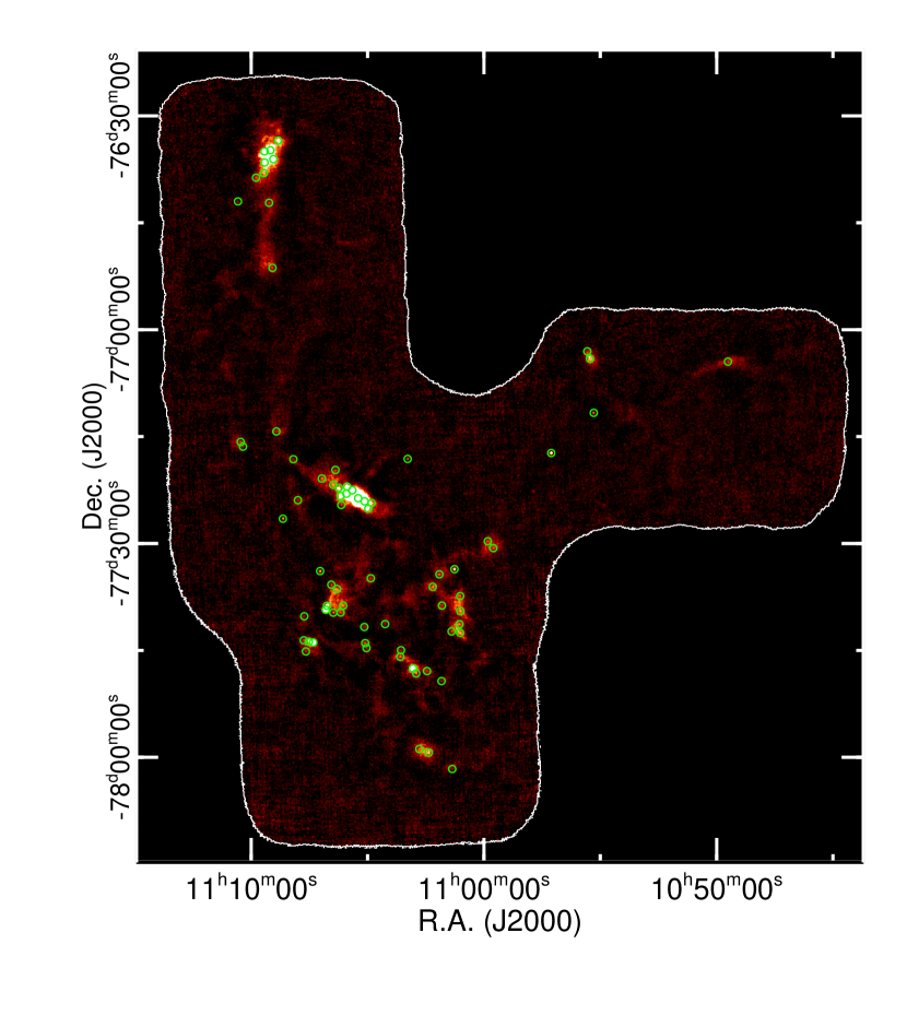
Figure 1.— APEX LABOCA 870 $\mu$m image of the Chamaeleon I cloud from Belloche et al. (2011b). The image is displayed on a linear scale ranging from $-$0.1 (black) to 0.15 (white) Jy beam^-1. The small green circles show the 73 ALMA pointings presented in this paper, with the diameters of the circles equal to the FWHM of the primary beam.

Sensitive interferometric surveys of large numbers of starless cores are required to make progress on improving detection statistics. Such surveys will constrain the level of substructure and fragmentation that develops in the starless core stage, and they will accurately determine the true number of starless cores, thus constraining both their lifetimes and the accretion luminosities and histories of the youngest protostars. With the advent of ALMA, such surveys are now possible. In this paper, we present the results of a Band 3 (106 GHz; 2.8 mm) ALMA Cycle 1 survey of all known dense cores in the Chamaeleon I molecular cloud, which is located at a distance of 150 pc (see discussion of distance in Belloche et al., 2011b). We target all 73 sources detected by Belloche et al. (2011b) in a single-dish 870 $\mu$m continuum survey with the Large Apex Bolometer Camera (LABOCA) at the Atacama Pathfinder Experiment (APEX). With ALMA’s exquisite sensitivity, our survey targets six times more cores to ten times better mass sensitivity than the Schnee et al. (2010) CARMA survey of Perseus cores in a fraction of the total observing time, and lays the groundwork for future surveys targeting similar populations in other star-forming clouds.

The organization of our paper is as follows: In §2, we describe the observations and data reduction. We present our basic results in §3, including a summary of the properties of the detected sources and an overview of the evolutionary status of each core, incorporating information from our ALMA observations. We discuss the implications of our results in §4 and §5, focusing on developing an accurate census of starless and protostellar cores in §4 and constraints on substructure and fragmentation in starless cores in §5. Finally, we summarize our results in §6.

2. Observations

We obtained ALMA observations of every source in Chamaleon I detected in the single-dish 870 $\mu$m LABOCA survey by Belloche et al. (2011b) except for those listed as likely artifacts (1 source), residuals from bright sources (7 sources), or detections tentatively associated with young stellar objects (3 sources). The first two categories were omitted to avoid unreliable sources, whereas the third category was omitted due to constraints on the maximum number of pointings allowed in a single observing program. Thus, we observed 73 sources from the initial list of 84 objects identified by Belloche et al. (2011b). Figure 1 shows the 73 ALMA pointings overlaid on the APEX LABOCA 870 $\mu$m image of Chamaeleon I presented by Belloche et al. (2011b).

We observed the 73 pointings using the ALMA Band 3 receivers during its Cycle 1 campaign between 2013 November 29 and 2014 March 08. Between 25 and 27 antennas were available for our observations, with the array configured in a relatively compact configuration to provide a resolution of approximately 2″ FWHM (300 AU at the distance to Chamaeleon I). Each target was observed in a single pointing with approximately 1 minute of on-source integration time. Three out of the four available spectral windows were configured to measure the continuum at 101, 103, and 114 GHz, each with a bandwidth of 2 GHz, for a total continuum bandwidth of 6 GHz (2.8 mm) at a central frequency of 106 GHz. These continuum observations achieved a 1$\sigma$ rms noise of approximately 0.1 mJy beam^-1. The remaining window was configured to observe the ¹²CO (1–0) line at 115 GHz. Only the continuum data are presented here. The maximum angular scale that can be recovered in these ALMA data is $\sim$25″.

The calibration and imaging were done using the Common Astronomy Software Applications (CASA) package following the standard routines described in Petry et al. (2014) and Schnee et al. (2014a). Additional refinement of the brightest continuum detections (those brighter than $\sim$3 mJy) was carried out through two rounds of self-calibration, the first phase-only and the second with amplitude and phase corrections. Overlapping fields were mosaiced together.

Table 1 lists, for each source, an identifier using the detection number from Belloche et al. (2011b), the phase center of our ALMA observations (taken directly from the core positions given by Belloche et al.), the FWHM size and position angle of our ALMA continuum synthesized beam, the 1$\sigma$ rms of our ALMA continuum data and corresponding 1$\sigma$ mass sensitivity, and a flag noting the evolutionary status of each source as determined by us (see discussion in §3.3 for more details regarding source evolutionary status). The 1$\sigma$ mass sensitivities are calculated assuming emission from optically thin, isothermal dust (see Equation 1 and accompanying text below for more details on this calculation).

3. Results

3.1. Continuum Detections: Observed and Physical Properties

With a pixel size of 0.25″, there are approximately 181,000 pixels over the primary beam (approximately 60″). With such a large number of pixels, Gaussian statistics predict over 500 pixels above 3$\sigma$ simply due to random noise, but $<$1 above 5$\sigma$. To avoid spurious detections, we thus adopt 5$\sigma$ as the minimum significance required for detection in this paper.

We detect a total of 24 106 GHz continuum sources to 5$\sigma$ or greater significance in 19 different target fields, leaving 54 target fields with no detections. Table 2 lists the name of each detected source (taken to be the same as the target field name) along with the results from an elliptical Gaussian fit to each source using the imfit task in CASA, including the source position, major and minor axes and position angle after deconvolution with the beam, peak flux density, and integrated flux density. All measurements were made on images corrected for primary beam attenuation. Fields with multiple sources detected append ‘A’, ‘B’, etc. to each source in alphabetical order with increasing Right Ascension. Sources found to be unresolved in one or both dimensions and thus unable to be deconvolved with the beam are noted.

Table 3 lists the physical properties of each detected source, including the effective radius, total mass, and mean total gas number density. The effective radius, $r_{eff}$, is calculated as the geometric mean of the semimajor and semiminor axes of the source, if beam deconvolution is possible, or the beam if not (in which case it is expressed as an upper limit). The mass is calculated as

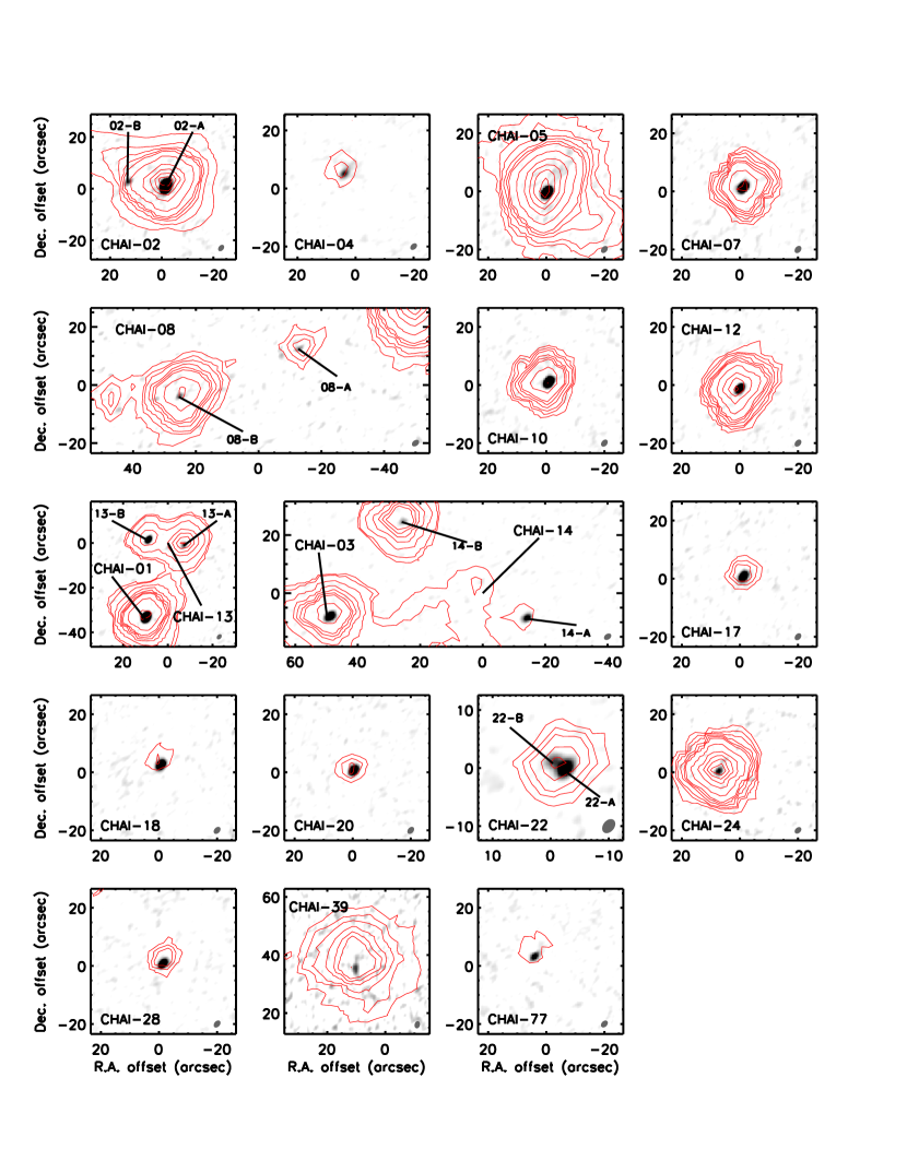
Figure 2.— Images of each source detected by our ALMA observations. The images are uncorrected for primary beam attenuation for display purposes. In each panel, the grayscale shows the ALMA 106 GHz continuum emission and the red contours show Herschel 70 $\mu$m emission from the Herschel Gould Belt survey, which were observed with a beam full-width at half-maximum (FWHM) of 8.4^′′ (Könyves et al., 2015). The gray ellipse at the lower right of each panel shows the ALMA synthesized beam. Each panel is labeled with the name of the target field in which the source is detected, with the coordinate offsets displayed relative to the core centers (which are also the phase centers of our observations; see Table 1). Panels covering multiple cores have the central positions of each core marked, and panels with multiple sources detected have each source labeled. The grayscale is plotted on a linear scale ranging from 0.1 (white) to 2 (black) mJy beam^-1 for each panel except CHAI-08, CHAI-24, and CHAI-39, where the maximum is instead 1 mJy beam^-1. In all panels except for five, the Herschel 70 $\mu$m contours are plotted at 10, 15, 20, 30, 40, 50, 100, 200, 300, 400, 500, 1000, 3000, 5000, 7000, and 9000 MJy sr^-1. For the following five panels, the same pattern is kept except with different minimum contour levels: CHAI-02 (100 MJy sr^-1), CHAI-13 and CHAI-14 (40 MJy sr^-1), and CHAI-18 and CHAI-77 (5 MJy sr^-1).

Figure 3.— Spectral energy distributions (SEDs) for each of the 24 sources detected by our ALMA 106 GHz continuum observations, based on associations with 2MASS, Spitzer, Herschel, and LABOCA sources. The associated 2MASS and Spitzer sources are taken from the YSO catalogs tabulated by the Spitzer Gould Belt Legacy Survey (Dunham et al., 2015), and the associated Herschel sources are taken from the Herschel Gould Belt Survey as tabulated by Winston et al. (2012). Each panel is labeled with the target field in which the source is detected. Fields with multiple detected sources have each SED separately plotted as filled circles and labeled when resolved, and the combined SED plotted with an x (and labeled) when unresolved. We do not include our ALMA continuum measurements since they may suffer from spatial filtering.

$$M=100\frac{d^{2}S_{\nu}}{B_{\nu}(T_{D})\kappa_{\nu}}\quad,$$ (1)

where $S_{\nu}$ is the integrated flux density, $B_{\nu}(T_{D})$ is the Planck function at the isothermal dust temperature $T_{D}$, $\kappa_{\nu}$ is the dust opacity, $d=150$ pc, and the factor of 100 is the assumed gas-to-dust ratio. We adopt the dust opacities of Ossenkopf & Henning (1994) appropriate for thin ice mantles after $10^{5}$ yr of coagulation at a gas density of $10^{6}$ cm^-3 (OH5 dust), giving $\kappa_{\nu}=0.23$ cm² g^-1 at 106 GHz. With the integrated flux densities listed in Table 2 and an assumed $T_{D}=10$ K, Equation 1 gives total masses ranging from 0.012 M_⊙ to 1.7 M_⊙. Note that the uncertainties listed in Table 3 only include the statistical uncertainties in the integrated flux densities. The true uncertainties are likely dominated by the dust temperature and opacity assumptions. As 3 mm is strongly in the Rayleigh-Jeans limit, a factor of two uncertainty in dust temperature directly translates into a factor of two uncertainty in mass. For the opacity, typical uncertainties of factors of $2-4$ are quoted based on the specific dust model (e.g., Shirley et al., 2005, 2011). However, the opacities can in fact be larger by an order of magnitude or more if dust grains have grown to millimeter sizes or larger, as such large grains will flatten the dust opacity power-law index (e.g., Ricci et al., 2010; Tobin et al., 2013; Testi et al., 2014; Schnee et al., 2014b). Shallower dust opacity power-law indices caused by larger grains would systematically increase the opacities compared to the assumed OH5 value, decreasing the calculated masses. While grains are not generally expected to grow to such large sizes in starless cores, Kwon et al. (2009) and Schnee et al. (2014b) did recently find evidence for large grains in both large-scale filaments and dense cores, although the Schnee et al. results have currently been questioned by Sadavoy et al. (2016). If large dust grains in dense starless cores are confirmed by future studies, the opacities assumed here will require upward revision.

The mean total gas number density, $n$, is calculated assuming spherical symmetry as

$$n=\frac{3}{4\pi\mu m_{H}}\frac{M}{r^{3}_{eff}}$$ (2)

where $M$ is the mass, $r_{eff}$ is the effective radius, $m_{H}$ is the hydrogen mass, and $\mu$ is the mean molecular weight per free particle. With $M$ and $r_{eff}$ as calculated above and $\mu=2.37$ for gas that is 71% by mass hydrogen, 27% helium, and 2% metals (Kauffmann et al., 2008), we calculate and tabulate number densities in the last column of Table 3. As with the mass, only the statistical uncertainties are listed in Table 3; the true uncertainties are dominated by systematic uncertainties in the assumed distance, source geometries, dust temperatures, and opacities, as discussed above.

Figure 2 shows images of each detected source overlaid with contours of the Herschel 70 $\mu$m emission from the Gould Belt survey (André et al., 2010; Winston et al., 2012). Figure 3 shows spectral energy distributions (SEDs) for each source constructed from 2MASS$+$Spitzer, Herschel, and LABOCA photometry tabulated by Dunham et al. (2013, 2015), Winston et al. (2012), and Belloche et al. (2011b), respectively. In the latter case the total flux densities rather than peak intensities are plotted. We do not include our ALMA 106 GHz continuum measurements in Figure 3 since they likely suffer from unknown levels of spatial filtering compared to the single-dish data.

3.2. Associations with Detections at Other Wavelengths

In order to investigate the nature of the continuum detections, we now consider their associations with sources detected at other wavelengths.

3.2.1 Association with LABOCA Sources

Column 2 of Table 4 lists the projected separation between each ALMA detection and the associated 870 $\mu$m LABOCA source targeted by our ALMA observations. We consider our sources to be physically associated with the corresponding LABOCA sources if they are located within a projected separation of 10.6″ (the half-power radius of the 21.2″ FWHM beam of the LABOCA observations; Belloche et al., 2011b). Associations following this definition are tabulated in column 3 of Table 4, showing that 18 of the 24 ALMA 106 GHz continuum detections are associated with LABOCA sources. Despite the ALMA detections of sources in the fields targeting CHAI-08, CHAI-14, and CHAI-39, these ALMA detections are located far enough away from the LABOCA sources themselves that we do not consider them to be physically associated with these sources.

3.2.2 Association with Herschel YSOs

Columns 4–6 of Table 4 list the YSO from Winston et al. (2012) associated with each detected source, along with the projected separation and evolutionary class (the latter taken directly from their Table 1). Winston et al. start with a list of 397 sources extracted from the Herschel 70–500 $\mu$m images of Chamaeleon I obtained as part of the Herschel Gould Belt Legacy Survey (André et al., 2010). They associated 49 of these Herschel detections with YSOs previously identified with Spitzer by Luhman et al. (2008) and list Herschel flux densities for those sources. All but two of our 106 GHz ALMA continuum detections are associated with these YSOs. One is a Class 0 object, five are Class I objects, four are flat-spectrum objects, 11 are Class II objects, and one is a transition disk (see Winston et al., 2012, for details). We thus detect all of the Class 0 and I YSOs listed by Winston et al. (2012), and four out of the six flat-spectrum objects. The remaining two flat-spectrum objects are not covered by our 73 ALMA pointings.

The two ALMA detections not associated with YSOs from Winston et al. (2012) are CHAI-02-B and CHAI-08-A. CHAI-02-B is located 13.5″ east of CHAI-02-A. Visual inspection of the Spitzer images provided by the Spitzer Gould Belt survey (Dunham et al., 2015) reveals a mid-infrared point source detected at 3.6-8 $\mu$m, and indeed it is listed as a flat-spectrum YSO by Luhman et al. (2008). It is not resolved into a separate source at Herschel wavelengths, explaining its absence from the Winston et al. (2012) catalog. CHAI-08-A is associated with a flat-spectrum YSO detected by Spitzer (Luhman et al., 2008), but it is not listed in the Winston et al. (2012) catalog.

3.2.3 Association with Spitzer Protostars

Columns 7–9 of Table 4 list the associated protostar from the Dunham et al. (2013) compilation of protostars detected by Spitzer in the Gould Belt clouds, including Chamaeleon I. This protostar catalog is a subset of the full Gould Belt YSO catalog presented by Dunham et al. (2015). Only 9 out of the 24 ALMA detections are associated with Spitzer-identified protostars. Dunham et al. (2013) emphasized reliability over completeness by requiring detections in all five Spitzer bands between 3.6–24 $\mu$m and association with dense cores as traced by complementary (sub)millimeter continuum surveys. Of the 15 ALMA detections that are not associated with protostars listed by Dunham et al. (2013), four are saturated at one or more wavelengths, three are near Spitzer map edges and thus not covered at one or more wavelengths, one is not detected at one or more wavelengths, three are not resolved at one or more wavelengths, and four are detected at all Spitzer wavelengths but not projected onto the positions of dense cores. We note here that the only Class 0 protostar in Chamaeleon I (CHAI-04, also known as Cha-MMS1) is not in the Dunham et al. catalog as it is not detected at all Spitzer wavelengths. Indeed, this object has been identified as a candidate first hydrostatic core (Larson, 1969; Belloche et al., 2006; Tsitali et al., 2013; Väisälä et al., 2014). Furthermore, two of the five Class I protostars in Chamaeleon I are also missing from the Dunham et al. catalog: CHAI-02-A due to saturation and CHAI-22-B due to not being resolved at all wavelengths. While Dunham et al. (2013) did acknowledge that their sample focuses on reliability at the expense of completeness, we emphasize here that the list of protostars in nearby clouds must continue to be updated as new information becomes available.

3.3. Evolutionary Status of the 73 Targets

The last column of Table 1 notes the evolutionary status of each of the 73 targets, determined as described below.

As noted above, 19 target fields feature continuum detections. Of those, the one associated with a Class 0 source (CHAI-04) and the four associated with Class I sources (CHAI-02, CHAI-05, CHAI-22, and CHAI-24) are clearly protostars, thus these objects are marked as protostellar cores. Eleven additional detections are associated (at least in projection) with LABOCA sources: CHAI-01, 03, 07, 10, 12, 13, 17, 18, 20, 28, and 77. However, as evident from Figure 3 and Column 6 of Table 4, all of these objects exhibit flat-spectrum or Class II SEDs indicative of more evolved objects near or beyond the end of the embedded, protostellar stage of evolution. One possible explanation for these sources being associated with LABOCA sources is that they are protostars viewed nearly face-on down outflow cavities, as such objects could exhibit Class II SEDs (e.g., Whitney et al., 2003; Dunham & Vorobyov, 2012). However, such objects tend to feature double-peaked SEDs (e.g., Whitney et al., 2003) not seen in Figure 3. Another, more likely possibility is that the associated LABOCA detections are not tracing dense cores. The Belloche et al. (2011b) LABOCA survey has a mass sensitivity more than six times deeper than surveys such as the Bolocam 1.1 mm surveys of nearby clouds (Enoch et al., 2006; Young et al., 2006; Enoch et al., 2007). It is also capable of recovering extended emission on scales up to a factor of 2–5 larger than other, previous surveys (see Appendix A of Belloche et al., 2011b, for a detailed discussion of spatial recovery). Thus, the LABOCA survey is more likely to detect both extended dust emission and dust in disks that are no longer embedded within dense cores, and indeed, for these reasons, Belloche et al. (2011b) never claimed all of their detections were tracing dense cores. While it is possible that some of these 11 LABOCA sources are evolved protostars near the end of the embedded stage (particularly the flat-spectrum sources; e.g., Heiderman & Evans, 2015), we classify these objects as disks rather than starless or protostellar dense cores. Finally, an additional three target fields contain detections that are too distant from the LABOCA sources themselves (which are located at the zero offset coordinates in Figure 2) to be considered associated: CHAI-08, 14, and 39. These detections are associated with other YSOs located within the ALMA primary beam, and the LABOCA sources themselves are considered starless cores.

With one exception, all other LABOCA sources not associated with any ALMA 106 GHz continuum detections are considered starless cores, leaving us with 56 starless cores, none of which are detected by our ALMA continuum observations. The one exception is CHAI-14: the two ALMA detections in this field are unassociated with the core, and the core itself is undetected. However, the LABOCA source is located at a projected distance of 3.6″ from a Class II YSO from the Winston et al. (2012) catalog. As this is well within the half-power point of the LABOCA beam, we classify CHAI-14 as a disk rather than a dense core, with our ALMA non-detection indicating a low-mass disk with a 3$\sigma$ mass limit of 4.2 $\times$ 10^-3 M_⊙ based on the mass sensitivity tabulated in Table 1.

4. A Complete Census of Star Formation in Chamaeleon I

As noted in §1, a number of very low luminosity protostars have been identified through interferometric detections of outflows and/or compact continuum emission from dense cores originally classified as starless (e.g., Enoch et al., 2010; Chen et al., 2010, 2012; Schnee et al., 2010, 2012; Pineda et al., 2011b; Dunham et al., 2011). For the most part, these newly identified protostars have been found serendipitously, raising the question of exactly how many “starless” cores are truly starless. In order to answer this question in Chamaeleon I we must first determine whether or not similar protostars would be detected in our observations. To address this, we take four such objects in the Perseus molecular cloud that have been observed with interferometers at millimeter wavelengths, with synthesized beams ranging from approximately 1^′′ to approximately 6^′′: L1448-IRS2E (Chen et al., 2010), Per-Bolo 45 (Schnee et al., 2010); Per-Bolo 58 (Enoch et al., 2010; Dunham et al., 2011), and L1451-mm (Pineda et al., 2011b). We then scale the observed peak intensities from 230 pc (the distance to Perseus, Hirota et al., 2008, 2011) to 150 pc (the distance to Chamaeleon I; see Belloche et al., 2011b, and references therein), as well as from the observed frequency to 106 GHz assuming $I_{\nu}\propto\nu^{2+\beta}$, where $\beta$ is the index of the dust opacity power-law through the far-infrared and (sub)millimeter wavelength range. The above expression is valid as long as the Rayleigh-Jeans limit ($h\nu<<kT$) is satisfied, which, for $\nu=106$ GHz, is satisfied for $T>>5.1$K. The sources are assumed to have the same dust temperatures in Chamaeleon I as in Perseus since we are simulating observing, at a different frequency, these exact sources in a cloud located at a different distance.

The results of scaling the observed peak intensities as described above, over the range $0\leq\beta\leq 2$, are given in Table 5 under the assumption that these observed peak intensities are dominated by compact, unresolved emission and thus independent of beam size. After scaling to the distance of Chamaeleon I, the predicted 106 GHz peak intensities range from 0.7 to 17.7 mJy beam^-1 depending on the source and the assumed value of $\beta$. As our sensitivities range from 0.08 to 0.14 mJy beam^-1, even in the most pessimistic scenario these objects would be detected to at least a 5$\sigma$ level, ranging to $>$200$\sigma$ in the most optimistic scenario. Robust detection of first hydrostatic cores is also predicted from the comparison with simulations presented below in the following section.

Based on these results, we conclude that the Spitzer$+$Herschel census of protostars in Chamaeleon I is complete and there are no missing protostars or first hydrostatic cores in this cloud. The one caveat to this statement is if low-mass, compact cores harboring protostars are missing from the Belloche et al. (2011b) catalog due to confusion with larger-scale emission, a possibility we cannot rule out here since, as seen in Figure 1, there are regions with detected 870 $\mu$m emission that are not covered by our ALMA pointings. If we assume that the Belloche et al. catalog is in fact complete, with 56 starless cores, we find that the rate at which protostellar cores in Chamaeleon I have been misclassified as starless cores is $<$1/56, or $<$ 2%.

5. Substructure and Fragmentation in Starless Cores

As noted in §1, if fragmentation begins in the starless core stage, it should be detectable by ALMA (Offner et al., 2012; Mairs et al., 2014). At first glance, our non-detections seem to imply that the starless cores in Chamaeleon I are not undergoing a process of turbulent fragmentation like that predicted in the simulations of Offner et al. (2010). However, the synthetic ALMA observations of the Offner et al. simulations presented by Offner et al. (2012) and Mairs et al. (2014) only examined selected times late in the evolution of the starless cores when they had already reached relatively high central densities and were close to the formation of central, hydrostatic objects. In order to fully examine the implications of our non-detections, we must determine how far back in time such starless cores are detectable and use these results to generate testable predictions for the number of detected cores expected in our sample. To accomplish this task, we revisit synthetic ALMA observations of the Offner et al. simulations, using updated simulations that include magnetic fields.

5.1. Synthetic ALMA Observations of Starless Core Simulations

5.1.1 Description of the Simulations

We perform two magneto-hydrodynamic (MHD) simulations of isolated, collapsing starless cores. The simulations are similar in their properties except for initial core masses that differ by one order of magnitude, with the lower mass simulation starting with an initial density 2.7 times higher (the higher density is required in order for this core to be sufficiently unstable to collapse). In the first simulation, which we label the C04 simulation, the initial core mass is 0.4 M_⊙. In the second, which we label the C4 simulation, the initial core mass is 4 M_⊙. We use the orion Adaptive Mesh Refinement (AMR) code to generate self-consistent, time-dependent physical conditions (Klein, 1999; Truelove et al., 1998; Li et al., 2012). The simulations include self-gravity and determine the gas temperature via a barotropic equation of state (EOS). The EOS models the transition from isothermal to adiabatic as the gas becomes optically thick to infrared radiation: the gas pressure is $P=\rho c_{s}^{2}[1+(\rho/\rho_{c})^{\gamma-1}]$, where $c_{s}$ is the sound speed, $\gamma=5/3$ is the ratio of specific heats, and $\rho_{c}=2\times 10^{-13}$ g cm^-3 is the critical density (Masunaga et al., 1998). orion evolves the magnetic field using a constrained transport ideal MHD scheme assuming the gas and magnetic field are perfectly coupled (Li et al., 2012), which is based on the finite volume formalism as implemented by Mignone et al. (2012).

The simulations begin with a uniform density spherical core of 10 K gas, with initial number densities of $1.6\times 10^{5}$ cm^-3 for the C04 simulation and $6.0\times 10^{4}$ cm^-3 for the C4 simulation. The core is surrounded by a warm, low density medium with a temperature of 1000 K and a density 100 times lower than the initial core density. The domain extent is twice the diameter of the core, and the domain edge has outflow boundary conditions. A uniform magnetic field threads the gas in the $z$ direction with a strength set such that the mass-to-flux ratio is five times the critical value. At $t=0$, the gas velocities in the core are perturbed with a turbulent random field, which has a flat power spectrum over wavenumbers $k=1-2$ and is normalized to satisfy the input velocity dispersion. Once set in motion, the initial turbulence is allowed to decay and no additional energy injection occurs. Table 6 summarizes the simulation properties.

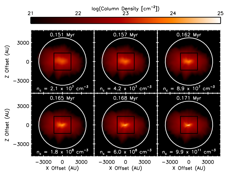
Figure 4.— Total gas column density snapshots for the last 0.02 Myr of evolution for simulation C04. Each panel is labeled with the time that has elapsed since the simulation began, and the central density of the core at that time. The last panel at 0.171 Myr is when a sink particle is inserted and the first hydrostatic core stage begins. The white circles show the ALMA 106 GHz primary beam assuming a distance of 150 pc, and the black squares show the central region displayed in Figure 6.

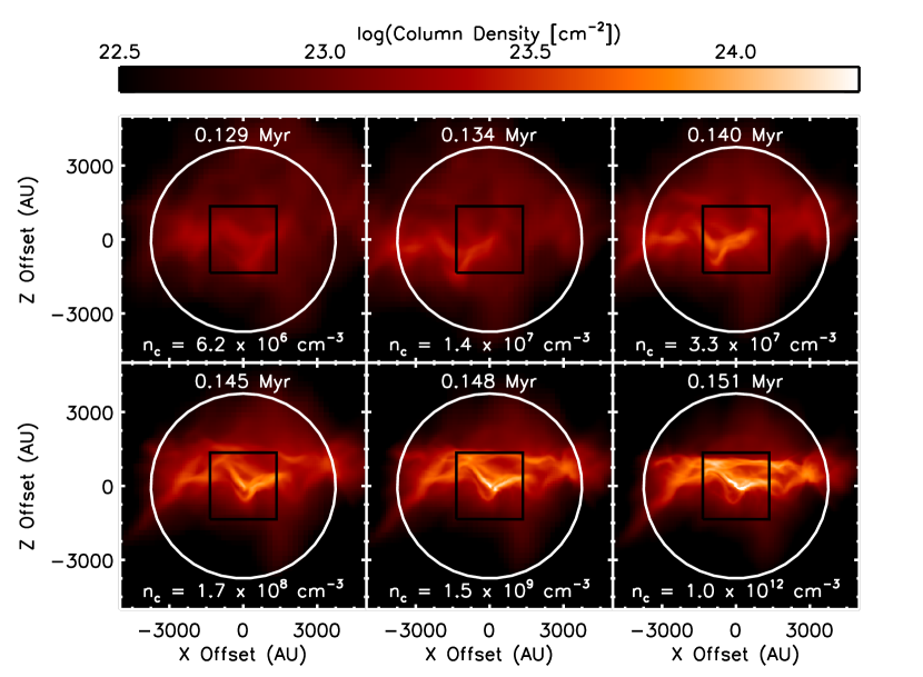
Figure 5.— Same as Figure 4, except for the last 0.022 Myr of evolution of the C4 simulation. The black squares show the central region displayed in Figure 7.

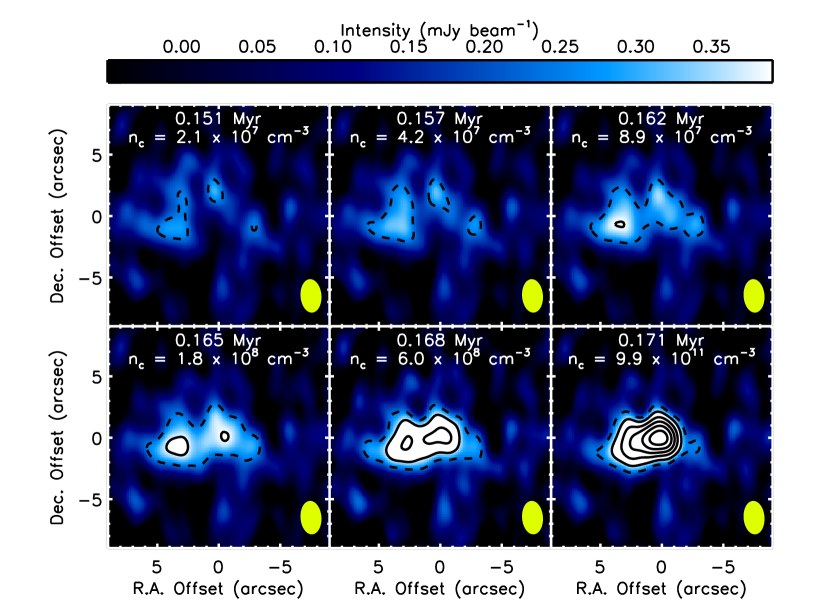
Figure 6.— Synthetic 106 GHz continuum observations of the C04 simulation at the same times shown above in Figure 4, matching the sensitivity and uv coverage of our ALMA Cycle 1 observations. Each panel is labeled with the time that has elapsed since the simulation began, and the central density of the core at that time. The beam is shown by the yellow ellipse at the lower right of each panel. The solid contours start at 5$\sigma$ and increase by 2$\sigma$, where 1$\sigma$ $\sim$ 0.1 mJy beam^-1, matching the sensitivity of our observations (see Table 1). The dashed contour plots the 3$\sigma$ level and is plotted as dashed to emphasize that it does not represent a robust detection.

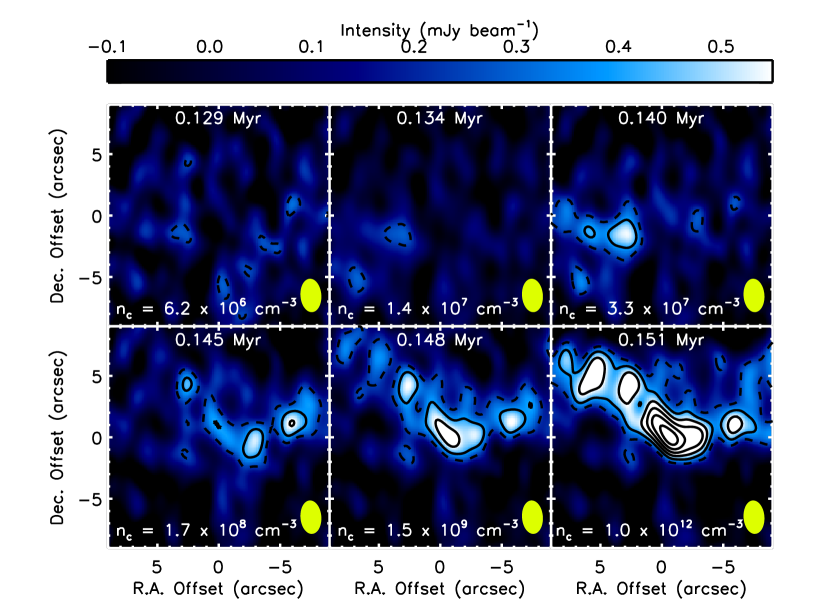
Figure 7.— Same as Figure 6, except for the last 0.022 Myr of evolution of the C4 simulation.

The initial basegrid resolution is $64^{3}$, but the dense core is refined by two additional levels via a density threshold refinement criterion. As the gas collapses, additional AMR levels are inserted when the density exceeds the Jeans condition for a Jeans number of $N_{J}=0.0625$ (Truelove et al., 1997). Each subsequent level increases the cell resolution by a factor of 2. When the Jeans condition is violated on the eighth level, a sink particle is added, representing the formation of a protostar (Krumholz et al., 2004). We evolve the calculation until shortly after the formation of a sink particle. At that time, the gas densities are comparable to those expected for the formation of a first hydrostatic core ($\rho=10^{-12}$ g cm^-3; see, e.g., Tomida et al., 2013).

Figures 4 and 5 show snapshots of the total gas column densities, $N$, from the two simulations, viewed perpendicular to the magnetic field (which is oriented in the $z$-direction). These snapshots focus on the last $\sim$0.02 Myr of evolution before the insertion of sink particles and onset of the first hydrostatic core stage. Since both simulations have the same number of AMR levels, the C04 core reaches higher densities before sink particle formation.

5.1.2 Description of the Synthetic Observations

To generate synthetic ALMA observations matching our Cycle 1 observations of the dense cores in Chamaeleon I, we begin with the total gas column density snapshots shown above. These snapshots are output on a fixed grid with a pixel size of 20 AU (0.13″ at the assumed distance of 150 pc), and converted to total gas surface density $\Sigma=\mu m_{H}N$, where $\mu$ and $m_{H}$ are the same as in Equation 2. While the Chamaeleon I dense cores are embedded within the larger cloud complex, the simulations are of isolated starless cores. This difference could affect our results since the cloud material will decrease the surface density contrast between the center and edge of the core. To account for this difference, we add a constant value of $\Sigma$ representing the background cloud material to every pixel. We consider the most extreme case by adopting a value of $\Sigma$ representing the maximum visual extinction toward the Chamaeleon I cloud of $A_{V}=35.6$, as measured in extinction maps with 2′ resolution. These maps were produced by the Spitzer c2d (Evans et al., 2009) and Gould Belt (Dunham et al., 2015) survey teams using 2MASS (Skrutskie et al., 2006) and Spitzer data (see Heiderman et al., 2010, for details). We convert this visual extinction to hydrogen column density using the relation $N_{H}/A_{V}=1.37\times 10^{21}$ cm^-2 (see Evans et al., 2009, for details), giving $N_{H}=4.88\times 10^{22}$ cm^-2. The total gas surface density is then calculated as $\Sigma=0.5\mu_{H_{2}}m_{H}N_{H}$, where $\mu_{H_{2}}$ is the mean molecular weight per hydrogen molecule ($\mu_{H_{2}}=2.8$; Kauffmann et al., 2008) and the factor of 0.5 accounts for the number of hydrogen atoms per hydrogen molecule, giving $\Sigma=0.114$ g cm^-2. Later tests showed that proceeding without adding this offset representing the large-scale cloud material gives identical results, as all of the large-scale emission is filtered out by the interferometer.

With the mass in each pixel calculated as $M=\Sigma A_{\rm pixel}$, where $A_{\rm pixel}$ is the area of each pixel ($A_{\rm pixel}=400$ ${\rm AU}^{2}=9.0\times 10^{28}$ ${\rm cm}^{2}$), we then generate 106 GHz continuum maps by inverting Equation 1 for flux density. For the temperature in each pixel we use empirically derived relationships between temperature and surface density derived from models of Bonnor-Ebert spheres (Bonnor, 1956; Ebert, 1955), as described in Appendix A. We use the same OH5 dust opacity as that used in Equation 1 (0.23 cm² g^-1; see the text after Equation 1 for a discussion of uncertainties in this assumed opacity).

We then generate synthetic ALMA observations of these simulated 106 GHz continuum intensity maps using the CASA tasks simobserve and simanalyze. We set the coordinates of the image centers to R.A. = 11:00:00, decl. = $-$77:20:00, representing the approximate center of the Chamaeleon I cloud. We use 1 s integration times and include thermal noise from the atmosphere. Matching our actual observations, for each core we observe a single pointing in the ALMA Cycle 1 configuration contained in the CASA configuration file alma.cycle1.3.cfg for a total of 72 s (on-source), at a central frequency of 106 GHz with a total bandwidth of 6 GHz. We then invert into the image plane and clean to a threshold of 0.3 mJy (approximately 3$\sigma$) using non-interactive cleaning with no specified clean mask.

Figures 6 and 7 show the resulting synthetic ALMA observations for the C04 and C4 simulations, respectively, at the same timesteps as shown above in the column density images. As with the column density snapshots shown above, these images are for cores viewed perpendicular to the magnetic field (which is oriented in the $z$-direction). For each simulation, the third panel (top right panel) shows the first timestep where the core is detected to at least 5$\sigma$, and the last panel (bottom right panel) shows the onset of the first hydrostatic core stage. The C04 simulation is detected over the last 8200 yr of the starless stage, when the central number density exceeds $8.9\times 10^{7}$ cm^-3. The C4 simulation is detected over the last 11000 yr of the starless stage, when the central number density exceeds $3.3\times 10^{7}$ cm^-3. We emphasize here that these detection thresholds are for cores viewed perpendicular to the magnetic field axis; the effects of viewing geometry on our results will be discussed below in §5.2.

Initially, it seems surprising that the central density thresholds for detection are similar despite a factor of ten difference in initial core mass. To further examine this situation, Figure 8 plots, at the first detected timestep for each simulation, the mass contained within given spatial scales. We calculate this by Fourier transforming images of the mass in each pixel calculated directly from the surface density maps, as described above, and then plotting the amplitude as a function of both spatial frequency $l$ (top axis) and spatial scale $r$ ($r=1/l$; bottom axis). This method mimics what an interferometer like ALMA actually sees, and shows that the amount of mass on compact ($\sim 1000$ AU) scales is similar between the two simulations even though the total mass on larger scales is different. The simulations considered here form compact structures with similar total masses when the cores reach similar central densities, regardless of the total mass reservoirs available in the cores.

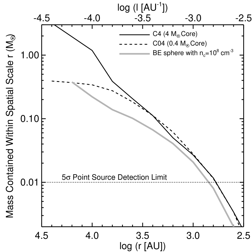
Figure 8.— Mass within various spatial scales versus those spatial scales for the C4 (solid black line) and C04 (dashed black line) simulations, calculated at the first timestep each simulation is detected in our synthetic ALMA observations. Also shown are the results for a Bonnor-Ebert sphere with a central density of $10^{8}$ cm^-3 (solid gray line; see Appendix A for details). The masses are calculated by Fourier transforming images of the mass in each pixel obtained from the surface density maps as described in the text. The dotted horizontal line shows the approximate 5$\sigma$ detection limit for point sources based on the sensitivities quoted in Table 1.

5.2. Detecting Starless Cores

Based on the results of the previous section, starless cores evolving under the Offner et al. (2010) turbulent fragmentation scenario should be detectable by our ALMA observations when they are viewed perpendicular to their magnetic field axes and their central number densities exceed between approximately $10^{7}$ cm^-3 and $10^{8}$ cm^-3, with the exact value depending on the mass of the core. As the mean mass of the starless cores in Chamaeleon I is 0.3 M_⊙ (Belloche et al., 2011b), we consider the C04 simulation to be more representative of Chamaeleon I cores. Thus, starless cores viewed perpendicular to their magnetic field axes should be detectable when their central number densities exceed $8.9\times 10^{7}$ cm^-3.

While we do not have any way to measure the central number densities of the starless cores in Chamaeleon I, Belloche et al. (2011b) derived lower limits by converting the single-dish LABOCA 870 $\mu$m peak intensities to peak masses according to Equation 1, and then calculating peak number densities using the effective radius of the beam. Their resulting values are $2.8-14.4~{}\times~{}10^{5}$ cm^-3, with a mean of $4.3\times 10^{5}$ cm^-3. As the peak intensities are beam-diluted by the LABOCA beam (FWHM of 21.2″, or 3180 AU at the distance to Chamaeleon I), the resulting peak number densities are lower limits to the true central number densities. Indeed, to demonstrate this, we generated 870 $\mu$m images of the simulations following the same procedure as described above for the 106 GHz (2.8 mm) images, convolved them with the 21.2″ FWHM LABOCA beam, and calculated peak number densities as described above, finding that the calculated peak number density remains constant at a few $\times 10^{5}$ cm^-3 as the central density increases from $10^{7}-10^{12}$ cm^-3. Thus we take the minimum calculated peak number density of $2.8~{}\times~{}10^{5}$ cm^-3 as a strong lower limit to the central number densities of the 56 starless cores in Chamaeleon I.

If we assume that Chamaeleon I has experienced a continuous rate of star formation over a timescale at least as long as the core lifetimes $\tau$, which are approximately $10^{6}$ yr (see below), then the expected number of detections can be calculated as:

$${\rm Detections}={\rm N_{total}}\times\frac{\tau_{\rm Detectable}}{\tau_{\rm Total}}\qquad,$$ (3)

where ${\rm N_{total}}$ is the total number of cores observed, $\tau_{\rm Detectable}$ is the lifetime over which cores are detectable, and $\tau_{\rm Total}$ is the total core lifetime. If we further assume that the cores evolve on free-fall timescales such that their lifetimes as a function of central number densities scale as $\tau\propto n^{-0.5}$, then Equation 3 can be written as:

$${\rm Detections}>{\rm N_{total}}\times\left(\frac{n_{\rm Detectable}}{n_{\rm Limit}}\right)^{-0.5}\qquad,$$ (4)

where $n_{\rm Detectable}$ is the central density threshold for detection and $n_{\rm Limit}$ is the observed lower limit for the central number densities of the cores. Note that the equation becomes an inequality since $n_{\rm Limit}$ is a lower limit. With N${}_{\rm total}=56$, n${}_{\rm Detectable}=8.9\times 10^{7}$ cm^-3, and n${}_{\rm Limit}>2.8\times 10^{5}$ cm^-3, Equation 4 results in a total of at least three expected detections.

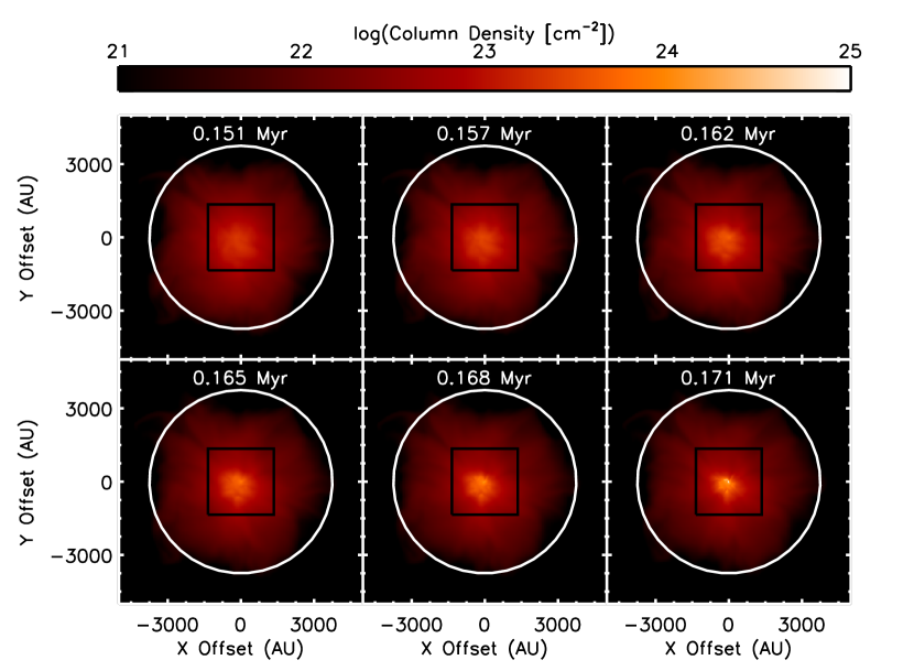
Figure 9.— Same as Figure 4, except viewed down the magnetic field axis.

As noted above, these results are derived using synthetic observations of simulated cores viewed perpendicular to their magnetic field axes. Since the cores tend to collapse along the magnetic field lines, they develop elongated, filamentary structure as they collapse. With this viewing geometry the elongated structure is seen edge-on, increasing the maximum column density observed at a given timestep. Indeed, Figure 9 shows column density snapshots for the C04 simulation at the same timesteps as shown in Figure 4, except viewed down the magnetic field axis (i.e., rotated 90^∘ compared to Figure 4). With this viewing geometry the cores exhibit less filamentary structure and lower column densities. After averaging over all possible orientations with respect to the line of sight, the total number of expected detections is reduced from at least three to at least two.

5.3. Implications of the 56 Non-Detections

Assuming Poisson statistics, the probability of detecting zero cores when two detections are expected is 13.5%. While there is thus a non-negligible chance that the non-detections are simply due to the sample size being too small, it is more likely that at least one of the assumptions adopted above are wrong. Here we evaluate each of these three assumptions, namely: (1) starless cores evolve on timescales proportional to the free-fall time, (2) star formation is continuous in Chamaeleon I, and (3) the simulations are applicable to the starless cores in Chamaeleon I.

5.3.1 Do Starless Cores Evolve on Timescales Proportional to the Free-Fall Time?

In order to evaluate whether or not starless cores evolve on timescales proportional to the free-fall time, meaning $\tau\propto n^{-0.5}$, Figure 10 plots the lifetime versus central number density (a so-called ‘JWT’ plot; Jessop & Ward-Thompson, 2000) for the C04 and C4 simulations. The lifetime at a given density is calculated as the amount of time it takes the simulation to evolve from the timestep with that central density to the onset of the first hydrostatic core phase. The C04 simulation, which is most appropriate for comparison to the cores in Chamaeleon I given their similar masses, lies between the $t_{\rm ff}$ and $10t_{\rm ff}$ lines but follows an identical slope, with a power-law fit giving $\tau~{}\propto~{}n^{-0.50\pm 0.01}$. A power-law fit to the C4 simulation gives $\tau~{}\propto~{}n^{-0.41\pm 0.01}$.

Also plotted in Figure 10 are observational determinations of $\tau$ vs. central number density for various samples from the literature, as compiled by Jessop & Ward-Thompson (2000) and Ward-Thompson et al. (2007). Visual inspection of the data suggests that core lifetimes normalized to free-fall times decrease as cores evolve to higher central densities, and indeed a power-law fit to all available data gives $\tau~{}\propto~{}n^{-0.69\pm 0.06}$. However, restricting the fit only to starless core populations with densities above $10^{4}$ cm^-3, densities more relevant for comparison to the high densities at which cores become detectable by our ALMA observations, the data follow the power-law $\tau~{}\propto~{}n^{-0.53\pm 0.11}$, consistent to within 1$\sigma$ with our assumption of evolution proportional to free-fall times. Thus we conclude that there is both observational and theoretical support for our assumption that starless cores evolve on timescales proportional to the free-fall timescale.

We note that, very recently, Könyves et al. (2015) found evidence that starless cores in Aquila evolve on faster timescales. While they don’t report the results of a power-law fit to $\tau$ vs. $n$, we estimate from their Figure 9 that the index of such a power-law is $\sim-0.9$ for central densities between $10^{5}$ cm^-3 and $10^{6}$ cm^-3. Inserting such a power-law index in Equation 4 would give much less than one expected detection. If future studies confirm the Könyves et al. (2015) results in additional clouds, then our assumption that $\tau\propto n^{-0.5}$ will require revisiting.

5.3.2 Is Star Formation Continuous in Chamaeleon I?

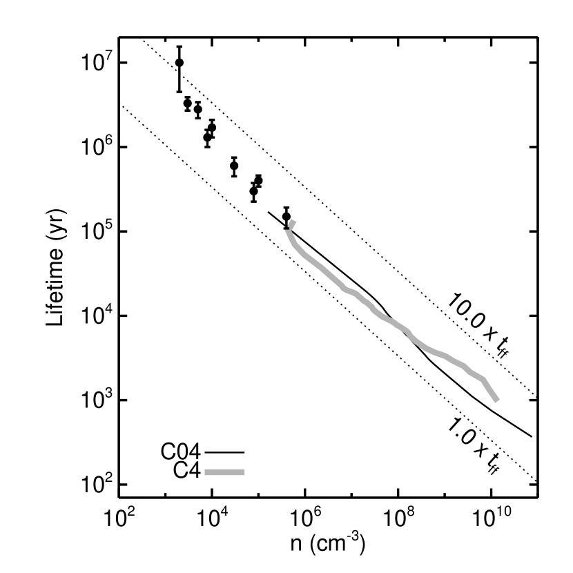
Figure 10.— Lifetimes versus central number densities for the C04 (thin black line) and C4 (thick gray line) simulations as they evolve. The lifetime at a given density is calculated as the amount of time it takes the simulation to evolve from the timestep with that central density to the onset of the first hydrostatic core phase. The dashed lines show the free-fall lifetime ($t_{\rm ff}=\sqrt{(3\pi)/(32G\rho)}$) and $10t_{\rm ff}$. The data points are taken from the literature as compiled by Jessop & Ward-Thompson (2000) and Ward-Thompson et al. (2007).

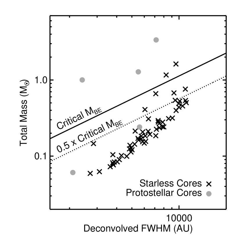
Figure 11.— Mass vs. size (deconvolved FWHM) for the starless (black x symbols) and protostellar (gray circles) cores in Chamaeleon I, taken from Belloche et al. (2011b). The solid line shows the critical Bonnor-Ebert mass ($M_{\rm BE}$), the maximum mass at a given radius for which a Bonnor-Ebert sphere is stable. The dotted line shows $0.5\times M_{\rm BE}$.

The assumption of continuous star formation means that starless cores form and collapse into stars at a constant rate. To test this assumption, we first examine the ratio of Class 0+I to Class II Young Stellar Objects in Chamaeleon I compared to other star-forming clouds. According to the results compiled by Dunham et al. (2015), this ratio is 0.06 for Chamaeleon I compared to 0.32 averaged over the 18 clouds observed by the Spitzer c2d (Evans et al., 2009) and Gould Belt (Dunham et al., 2015) Legacy Surveys. Thus, Chamaeleon I is deficient in the fraction of the youngest protostars compared to other, nearby molecular clouds, possibly indicating a decelerating rate of star formation, a point also noted by Belloche et al. (2011b).

To further test the assumption of continuous star formation, Figure 11 plots the mass versus size for the starless and protostellar cores in Chamaeleon I, as tabulated by Belloche et al. (2011b). Overplotted are lines showing the maximum mass at a given radius for which a Bonnor-Ebert sphere (Bonnor, 1956; Ebert, 1955) is stable, and 0.5 times this maximum mass (to account for the typical factor of $\sim$2 uncertainty in mass calculations). Belloche et al. (2011b) present a very similar figure (their Figure 9b) and argue that most of the starless cores in Chamaeleon I are in fact stable and not currently collapsing, and thus not evolving to form stars at a constant rate.

Belloche et al. (2011b) combine the above two arguments - namely a low protostar fraction and low fraction of unstable starless cores - with a measured high global star formation efficiency to argue that Chamaeleon I has a declining star formation rate and is nearly finished forming stars. Such a scenario may be explained if Chamaeleon I is globally unbound due to turbulence, as such a cloud would produce a population of starless cores that would not collapse further (Clark & Bonnell, 2004). In this scenario, most of the remaining starless cores will never form stars. While Naranjo Romero et al. (2015) present a scenario in which collapsing starless cores can appear stable when compared to their critical Bonnor-Ebert masses, other authors find that applying the critical Bonnor-Ebert stability criterion overpredicts the number of unstable cores (e.g., Pattle et al., 2015). Furthermore, Tsitali et al. (2015) found that only five of the starless cores in Chamaeleon I (9%) are bound, and only 13–28% show kinematic signatures of infall. We note that many of these cores, which are typically located in large-scale, filamentary cloud structures, could accrete more mass and thus become unstable in the future. While Belloche et al. (2011b) argue against this based on the low mass-to-length ratios of the filaments, the filaments themselves could still be gaining mass from the surrounding cloud. Indeed, further analysis by Belloche et al. (2011a) suggested that up to 50% of the starless cores in Chamaeleon I could eventually go on to form stars.

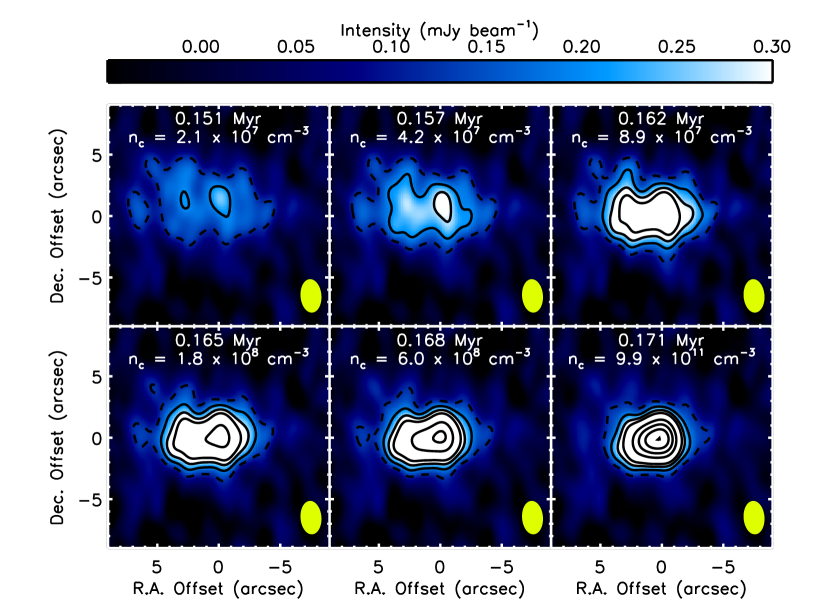
Figure 12.— Same as Figure 6, except with four times longer total integration time. The dashed contour plots the 3$\sigma$ level, where 1$\sigma$ $\sim$ 0.05 mJy beam^-1, and is plotted as dashed to emphasize that it does not represent a robust detection. The first three solid contours plot 5$\sigma$, 7$\sigma$, and 9$\sigma$ emission. The remaining contours start at 15$\sigma$ and increase in increments of 5$\sigma$.

Given the above evidence, the assumption of continuous star formation in Chamaeleon I is likely wrong. Instead, the star formation rate in this cloud is declining and most of the starless cores currently observed are not collapsing. Whether or not star formation is truly ending or simply pausing remains an open question. Either way, since the simulations are collapsing at all times, N_total in Equations 3 and 4 should be the total number of collapsing starless cores. Reducing this number by more than a factor of two would decrease the lower limit to the number of expected detections to below one. Thus our non-detections may be fully explained by a false assumption of continuous star formation.

5.3.3 Are the Simulations Applicable?

Even if all of the starless cores in Chamaeleon I are collapsing, which evidence suggests is not the case (as discussed above), a third possibility is that the simulations themselves are not applicable to these starless cores in terms of their initial conditions or physical treatment. As noted in Table 6, the simulations start with initial velocity dispersions between 0.16–0.26 km s^-1. These values are dominated by turbulent motions that are damped as the cores collapse, leading to lower values at the times the cores are actually detectable. For example, the velocity dispersion in the C04 simulation decreases from 0.16 km s^-1 at early times to $\sim$0.1 km s^-1 just prior to the formation of the first core. These velocity dispersions are in good agreement with those recently measured for the Chamaeleon I starless cores by Tsitali et al. (2015). However, it is still possible that the simulations are not applicable to the Chamaeleon I starless cores.

As an alternative to the simulations considered here, Appendix A shows that starless cores collapsing as Bonnor-Ebert spheres (Bonnor, 1956; Ebert, 1955) remain undetected to central densities at least as high as $10^{10}$ cm^-3. Inserting $n_{\rm Detectable}~{}>~{}10^{10}$ cm^-3 in Equation 4 results in a lower limit to the number of expected detections of much less than one. While this could also explain our non-detections, we are unable to distinguish between the simulations and Bonnor-Ebert spheres due to the fact that most of the cores are likely not collapsing, as discussed above.

While our survey of the starless cores in Chamaeleon I is an important step toward understanding when substructure and fragmentation develop in collapsing molecular cloud cores, further work is needed on both the observational and theoretical fronts. On the theoretical side, a full parameter space exploration is required to test how the development of substructure and fragmentation depends on initial core mass, turbulence, magnetic field strength, and viewing geometry.

On the observational side, the first step required is improved statistics. If all of the cores are indeed collapsing, increasing the total number of cores observed by a factor of three would increase the number of expected detections from two to six, reducing the probability of zero detections from 13.5% to 0.2% (assuming Poisson statistics). Furthermore, as shown in Figure 12, integrating to two times deeper mass sensitivity would reduce the central density detection threshold by approximately a factor of four, doubling the number of expected detections. We thus recommend that future surveys of starless cores be conducted with ALMA, and that these surveys integrate to twice the mass sensitivity obtained here in order to maximize their statistical power. Finally, beyond simply improving the statistics, future surveys should also focus on surveying starless cores that are likely to be unstable and thus collapsing, and on characterizing variations in the levels of substructure and fragmentation with different core properties, including their mass and level of turbulence. Only with such full parameter space study can different models of collapsing cores be distinguished.

6. Summary

In this paper, we have presented the results from a Band 3 (3 mm), ALMA Cycle 1 survey of 73 sources in Chamaeleon I previously identified in a single-dish 870 $\mu$m continuum survey. We summarize our main results as follows:

1. We detect a total of 24 106 GHz continuum sources in 19 different target fields, leaving 54 target fields with no detections. We calculate and tabulate the effective radius, total gas mass, and mean total gas number density for each detected source.

2. We tabulate associations between our continuum detections and sources detected by LABOCA, YSOs detected by Herschel, and protostars detected by Spitzer. We compile SEDs for each detection and use the results to assign a final evolutionary status to each of the 73 targets, identifying 56 targets as starless cores.

3. All previously known Class 0 and Class I protostars in Chamaeleon I are detected in our continuum observations. All other detections are associated with more evolved Flat-spectrum or Class II YSOs.

4. Very low luminosity protostars or first hydrostatic cores below the sensitivities of Spitzer and Herschel would have been detected to at least $5\sigma$ significance under even the most pessimistic assumptions, based on comparing to both simulations and to similar objects previously detected in the Perseus molecular cloud. Our results thus indicate that the Spitzer+Herschel census of protostars in Chamaeleon I is complete, with the rate at which protostellar cores have been misclassified as starless cores calculated as $<$1/56, or $<$2%.

5. Synthetic observations of magneto-hydrodynamical simulations of collapsing starless cores following the turbulent fragmentation scenario are detectable by these ALMA observations, but only over relatively short time periods when their central densities exceed $\sim$10⁸ cm^-3, with the exact density dependent on the viewing geometry. Bonnor-Ebert spheres, on the other hand, remain undetected to central densities at least as high as $10^{10}$ cm^-3.

6. Assuming that the turbulent fragmentation simulations accurately describe the collapse of starless cores in Chamaeleon I, that star formation is continuous and all of the starless cores in Chamaeleon I are collapsing, and that cores evolve on timescales proportional to their free-fall times, our sample of 56 starless cores, all with central densities above $2.8~{}\times~{}10^{5}$ cm^-3, should have yielded at least two detections.

7. Assuming Poisson statistics, there is a 13.5% probability of zero detections if the above assumptions are correct. Thus, while it is possible that our non-detections result from a sample size that is too small, it is more likely that at least one of the above assumptions are wrong. The most likely culprit is the assumption of continuous star formation; instead, evidence suggests that the star formation rate in Chamaeleon I is declining and most of the starless cores are not currently collapsing. It is also possible that the cores are more accurately described by models that develop less substructure than the simulations considered here, such as Bonnor-Ebert spheres.

With the advent of ALMA, surveys of the complete populations of starless cores in molecular clouds with sufficient sensitivity to detect substructure and fragments have now become accessible. We have demonstrated the feasibility and usefulness of such surveys with this work targeting the dense core population of Chamaeleon I. Future work should target additional clouds in order to improve the statistics and better constrain the validity of the turbulent fragmentation scenario in the evolution of starless cores and origin of multiple systems. Surveys of additional clouds are also needed to fully determine the fraction of protostellar cores that have been misclassified as starless given the vastly different fractions determined here for Chamaeleon I ($<$2%) and previously by Schnee et al. (2012) for Perseus (possibly as high as 20%).

Appendix A A.  Bonnor-Ebert Spheres

In this appendix we assess the detectability of Bonnor-Ebert spheres (pressure-truncated, self-gravitating spheres; Bonnor, 1956; Ebert, 1955) in our ALMA observations. We constructed Bonnor-Ebert (hereafter BE) density profiles for central densities ranging from $10^{5}$ cm^-3 to $10^{10}$ cm^-3, truncated at 7000 AU to approximately match the mean FWHM of 6600 AU for the starless cores in Chamaeleon I, based on the sizes measured by Belloche et al. (2011b). We then solved for the temperature profiles in each BE sphere using the three-dimensional Monte Carlo radiative transfer package RADMC-3D (Dullemond & Turolla, 2000; Dullemond & Dominik, 2004) in its 1-D, spherically symmetric mode. The cores are heated externally by the interstellar radiation field (ISRF). We adopt the Black (1994) ISRF, modified in the ultraviolet to reproduce the Draine (1978) ISRF, and then extincted by a given $A_{V}$ of dust with properties given by Draine & Lee (1984) to simulate extinction by the surrounding lower density environment. Further discussion of this adopted ISRF is given by Evans et al. (2001). For the radiative transfer calculations, we adopt the dust opacities of Ossenkopf & Henning (1994) appropriate for thin ice mantles after $10^{5}$ yr of coagulation at a gas density of $10^{6}$ cm^-3 (OH5 dust), and include isotropic scattering off dust grains.

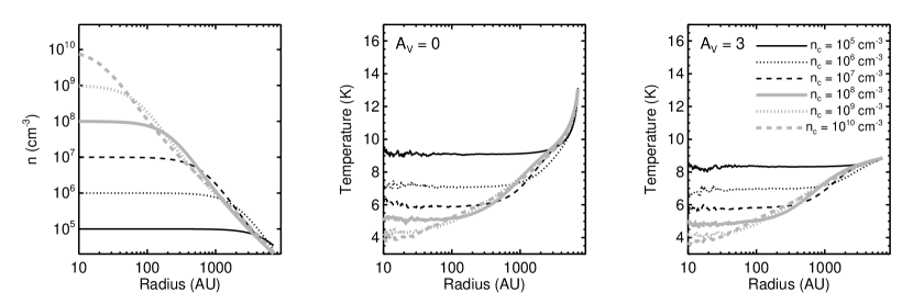
Figure 13.— Density and temperature profiles for the Bonnor-Ebert (BE) spheres considered here. Left: Total gas number density profiles for BE spheres ranging in central densities from $10^{5}$ cm^-3 to $10^{10}$ cm^-3, truncated at 7000 AU. Middle: Temperature profiles calculated by RADMC-3D for the case of no attenuation of the interstellar radiation field (ISRF; see text for details). Right: Temperature profiles calculated by RADMC-3D for the case of attentuation of the ISRF by $A_{V}=3$ of dust with properties given by Draine & Lee (1984). The figure key given in the right panel applies to all three panels.

Figure 13 plots the number density and temperature profiles for these BE spheres, where the latter are calculated by RADMC-3D and agree with those calculated by Evans et al. (2001). Two different temperature profiles are shown, one set for no attenuation of the ISRF ($A_{V}=0$) and one set for attenuation of the ISRF by $A_{V}=3$ of dust. As expected, the attenuated ISRF results in generally cooler temperature profiles, with less contrast between the dust temperatures at the centers and the outer edges. For all of the following analysis, we consider only the case with $A_{V}=3$; identical results on detectability were obtained with the $A_{V}=0$ case. Figure 14 shows images of the total gas column density for the six different BE spheres considered here.

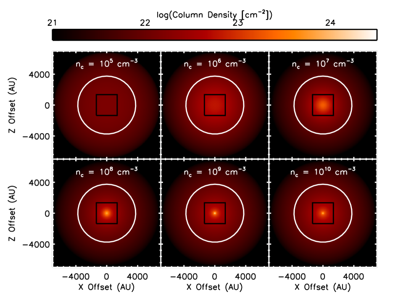
Figure 14.— Total gas column density for Bonnor-Ebert spheres ranging in central density from $10^{5}$ cm^-3 to $10^{10}$ cm^-3 and truncated to radii of 7000 AU. The white circles show the ALMA 106 GHz primary beam assuming a distance of 150 pc, and the black squares show the central region displayed in Figure 15.

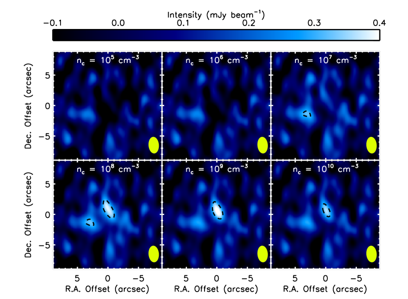
Figure 15.— Synthetic 106 GHz continuum observations of Bonnor-Ebert spheres ranging in central density from $10^{5}$ cm^-3 to $10^{10}$ cm^-3 and truncated to radii of 7000 AU, matching the sensitivity and uv coverage of our ALMA Cycle 1 observations. The beam is shown by the yellow ellipse at the lower right of each panel. The solid contours start at 5$\sigma$ and increase by 2$\sigma$, where 1$\sigma$ $\sim$ 0.1 mJy beam^-1, matching the sensitivity of our observations (see Table 1). The dotted contour plots the 3$\sigma$ level and is plotted as dashed to emphasize that it does not represent a robust detection.

To generate synthetic ALMA observations matching our Cycle 1 observations of dense cores in Chamaeleon I, we use RADMC-3D to generate model images at 106 GHz. We then generate synthetic ALMA observations of these model images following the same procedure as described above in §5.1.2: using the CASA tasks simobserve and simanalyze, we set the image center to coordinates matching the approximate center of the Chamaeleon I cloud and observe each model for a total of 72 s on-source in 1 second integrations with 6 GHz of bandwidth, using the ALMA Cycle 1 configuration contained in the CASA configuration file alma.cycle1.3.cfg. We include thermal noise from the atmosphere and clean to a threshold of 0.3 mJy (approximately 3$\sigma$) using non-interactive cleaning with no specified clean mask.

Figure 15 shows the resulting synthetic ALMA observations for the six different BE spheres. While there are 3$\sigma$ detections associated with the BE spheres with $n_{c}\geq 10^{8}$ cm^-3, there are no 5$\sigma$ detections, not even for the $n_{c}=10^{10}$ cm^-3 model. Thus, using the 5$\sigma$ detection threshold discussed above, Bonnor-Ebert spheres would remain undetected to central densities at least as high as $10^{10}$ cm^-3.

Inserting $n_{\rm Detectable}~{}>~{}10^{10}$ cm^-3 into Equation 4 while leaving $N_{\rm total}~{}=~{}56$ and $n_{\rm Limit}~{}>~{}2.8~{}\times~{}10^{5}$ cm^-3 yields an expectation of less than one detection. To understand these results, we note that the masses on various spatial scales shown in Figure 8, calculated via Fourier transforms of images of the mass in each pixel as described above, show that a BE sphere with a very similar central density to that of the C04 simulation when it is first detected ($10^{8}$ cm^-3 for the BE sphere versus $8.9~{}\times~{}10^{7}$ cm^-3 for the C04 simulation) has less mass on scales of several hundred AU to several thousand AU despite comparable total masses. Future surveys targeting larger numbers of starless cores in different environments are needed to fully distinguish between the levels of substructure and fragmentation predicted by Bonnor-Ebert spheres and those predicted by the Offner et al. (2010) turbulent fragmentation simulations.

Inspection of Figure 13 shows that our model Bonnor-Ebert spheres reach very cold temperatures in their centers, as low as $4-5$ K for the models with $n_{c}\geq 10^{8}$ cm^-3. While the BE sphere models presented by Evans et al. (2001) only reached minimum central temperatures of $6-7$ K, they only considered models with central densities up to $10^{7}$ cm^-3, thus our results are in fact consistent. We acknowledge that our models only consider external heating from the interstellar radiation field while neglecting other sources of heating, including cosmic ray heating. By setting a temperature floor of 7 K and then regenerating the synthetic ALMA images shown in Figure 15, we find that the Bonnor-Ebert spheres produce 5$\sigma$ detections for $n_{c}>10^{8}$ cm^-3.

However, while the neglected additional sources of heating could increase the central temperatures, Evans et al. (2001) showed that, for dust temperatures as low as at least 5 K, external heating from the interstellar radiation field dominated over the sum of direct heating of dust by cosmic rays, heating of dust by ultraviolet photons created following cosmic ray ionization of H₂, and heating of dust by collisions with gas heated by cosmic rays. Thus, we argue that our low temperatures, and resulting predictions that BE spheres remain undetected to central densities at least as high as $10^{10}$ cm^-3, are likely realistic.

Figure 16.— $\bar{T_{d}}$, the weighted mean dust temperature along each line of sight, versus the column density along that same line of sight. The six panels show the relationships for BE spheres ranging from $10^{5}$ cm^-3 to $10^{10}$ cm^-3, with each panel labeled in the lower left corner.

Finally, we use these Bonnor-Ebert spheres to develop empirical relationships between column density and dust temperature, and use these relationships to assign dust temperatures to each pixel of the column density snapshots of the simulations (as described in §5.1.2). For each of the six BE sphere models considered here, in each pixel of the column density maps shown in Figure 14 we calculate the mean dust temperature along the line-of-sight, weighted by the mass at each temperature. In practice this weighted mean dust temperature, $\bar{T_{d}}$, is calculated as

$$\bar{T_{d}}=\frac{\int T(s)\,n(s)\,ds}{\int n(s)\,ds}\qquad,$$ (A1)

where $s$ is the distance along the line of sight. Figure 16 shows the resulting relationships between column density and dust temperature for each of the six BE sphere models. When assigning dust temperatures to each pixel in the column density images from the simulations, we select the BE sphere model with the closest maximum column density to that found in each timestep of the simulation and interpolate using the relationships shown in Figure 16 to assign a dust temperature to each value of the column density.

While dust temperatures below 10 K have been observed in starless cores (e.g., Evans et al., 2001; Bergin et al., 2006), these empirical relationships between column density and dust temperature are derived for BE spheres and may not be generally applicable to the simulations considered here. However, our results are only weakly sensitive to the exact temperature model adopted. If, for example, we used the same model except with the addition of a 7 K temperature floor, the minimum central density at which the C04 simulation is detected decreases by a factor of three, from $n_{c}~{}=~{}8.9~{}\times~{}10^{7}$ cm^-3 to $n_{c}~{}=~{}3.2~{}\times~{}10^{7}$ cm^-3 (when viewed perpendicular to the magnetic field axis). As a result, the total number of expected detections, averaged over all possible orientations of the magnetic field with respect to the line of sight, increases from at least two to at least three.

Table 1ALMA 106 GHz Continuum Observations

			Synthesized	Synthesized
	R.A.	Decl.	Beam Size	Beam P.A.	1$\sigma$ rms	$\sigma_{M}$	Evolutionary
Source	(J2000)	(J2000)	(arcseconds)	(degrees)	(mJy beam-1)	(M⊙ beam-1)	Status
CHAI-01	11:08:03.22	$-$77:39:17.9	$2.72\times 1.89$	$-$40.2	0.12	0.0021	D
CHAI-02	11:08:38.96	$-$77:43:52.9	$2.75\times 1.92$	$-$40.0	0.12	0.0021	P
CHAI-03	11:10:00.13	$-$76:34:59.1	$2.67\times 1.89$	$-$42.4	0.11	0.0019	D
CHAI-04	11:06:31.94	$-$77:23:38.9	$2.62\times 1.82$	$-$46.6	0.08	0.0014	P
CHAI-05	11:06:46.44	$-$77:22:32.2	$2.71\times 1.89$	$-$40.7	0.12	0.0021	P
CHAI-06	11:06:15.51	$-$77:24:04.9	$2.61\times 1.82$	$-$44.8	0.08	0.0014	S
CHAI-07	10:58:16.92	$-$77:17:18.3	$2.74\times 1.97$	$-$39.2	0.12	0.0021	D
CHAI-08	11:07:01.85	$-$77:23:00.8	$2.61\times 1.82$	$-$45.6	0.08	0.0014	S
CHAI-09	11:04:16.41	$-$77:47:32.1	$2.63\times 1.82$	$-$44.8	0.08	0.0014	S
CHAI-10	11:02:24.98	$-$77:33:36.3	$2.70\times 1.89$	$-$38.7	0.12	0.0021	D
CHAI-11	11:08:50.40	$-$77:43:46.7	$2.63\times 1.82$	$-$45.0	0.09	0.0016	S
CHAI-12	11:08:15.28	$-$77:33:51.9	$2.72\times 1.89$	$-$40.6	0.11	0.0019	D
CHAI-13	11:08:00.07	$-$77:38:43.8	$2.60\times 1.83$	$-$41.5	0.10	0.0018	D
CHAI-14	11:09:45.85	$-$76:34:49.7	$2.59\times 1.82$	$-$47.9	0.08	0.0014	D
CHAI-15	11:06:59.93	$-$77:22:00.6	$2.61\times 1.82$	$-$45.9	0.08	0.0014	S
CHAI-16	10:56:42.95	$-$77:04:05.1	$2.58\times 1.82$	$-$43.5	0.08	0.0014	S
CHAI-17	10:56:30.56	$-$77:11:39.8	$2.65\times 1.89$	$-$38.8	0.11	0.0019	D
CHAI-18	11:09:47.42	$-$77:26:31.5	$2.73\times 1.89$	$-$42.4	0.11	0.0019	D
CHAI-20	11:07:21.34	$-$77:22:12.1	$2.72\times 1.89$	$-$41.4	0.11	0.0019	D
CHAI-21	11:06:06.48	$-$77:25:06.7	$2.61\times 1.82$	$-$44.6	0.08	0.0014	S
CHAI-22	11:04:23.35	$-$77:18:07.8	$2.69\times 1.89$	$-$39.2	0.12	0.0021	P
CHAI-23	11:02:10.85	$-$77:42:31.8	$2.59\times 1.82$	$-$40.4	0.09	0.0016	S
CHAI-24	11:09:26.24	$-$76:33:28.3	$2.58\times 1.82$	$-$47.1	0.08	0.0014	P
CHAI-25	11:03:36.59	$-$77:59:19.3	$2.64\times 1.82$	$-$44.1	0.08	0.0014	S
CHAI-26	11:07:17.13	$-$77:23:20.2	$2.60\times 1.82$	$-$44.5	0.08	0.0014	S
CHAI-28	11:07:43.89	$-$77:39:41.6	$2.73\times 1.89$	$-$40.9	0.12	0.0021	D
CHAI-29	11:10:01.05	$-$76:36:32.9	$2.57\times 1.82$	$-$46.3	0.08	0.0014	S
CHAI-30	11:06:21.67	$-$77:43:58.4	$2.51\times 1.80$	$-$13.9	0.12	0.0021	S
CHAI-32	11:03:21.97	$-$77:36:04.4	$2.50\times 1.80$	$-$13.6	0.13	0.0023	S
CHAI-33	11:04:49.58	$-$77:45:53.5	$2.51\times 1.80$	$-$13.7	0.13	0.0023	S
CHAI-34	11:03:39.07	$-$77:47:54.0	$2.51\times 1.80$	$-$13.5	0.13	0.0023	S
CHAI-35	11:11:27.78	$-$77:15:45.2	$2.48\times 1.80$	$-$17.0	0.13	0.0023	S
CHAI-36	11:04:07.89	$-$77:48:13.1	$2.51\times 1.80$	$-$13.0	0.13	0.0023	S
CHAI-37	11:04:01.79	$-$77:58:50.4	$2.52\times 1.80$	$-$12.1	0.13	0.0023	S
CHAI-38	11:03:04.43	$-$77:34:19.4	$2.50\times 1.80$	$-$12.4	0.13	0.0023	S
CHAI-39	11:07:17.30	$-$77:38:42.3	$2.50\times 1.80$	$-$14.4	0.13	0.0023	S
CHAI-40	11:09:03.86	$-$77:43:34.6	$2.51\times 1.80$	$-$13.9	0.13	0.0023	S
CHAI-41	11:02:10.46	$-$77:37:22.9	$2.50\times 1.80$	$-$11.0	0.13	0.0023	S
CHAI-42	11:09:39.48	$-$76:36:04.6	$2.44\times 1.80$	$-$16.4	0.14	0.0025	S
CHAI-43	11:07:47.07	$-$77:35:46.8	$2.50\times 1.80$	$-$12.7	0.13	0.0023	S
CHAI-44	11:05:57.64	$-$77:24:18.9	$2.49\times 1.80$	$-$13.5	0.13	0.0023	S
CHAI-45	11:00:43.98	$-$77:30:38.5	$2.49\times 1.80$	$-$11.4	0.13	0.0023	S
CHAI-46	11:00:58.29	$-$77:29:41.2	$2.59\times 1.89$	$-$24.8	0.11	0.0019	S
CHAI-47	11:07:32.72	$-$77:36:23.0	$2.61\times 1.89$	$-$27.8	0.11	0.0019	S
CHAI-49	11:02:33.40	$-$77:42:20.1	$2.61\times 1.89$	$-$25.6	0.11	0.0019	S
CHAI-50	10:50:56.54	$-$77:04:29.1	$2.56\times 1.89$	$-$22.0	0.11	0.0019	S
CHAI-52	11:09:15.17	$-$77:18:10.7	$2.59\times 1.89$	$-$26.7	0.11	0.0019	S
CHAI-53	11:06:23.17	$-$77:41:42.7	$2.61\times 1.89$	$-$26.7	0.11	0.0019	S
CHAI-54	11:09:56.09	$-$77:14:16.7	$2.59\times 1.89$	$-$27.5	0.11	0.0019	S
CHAI-55	11:02:10.12	$-$77:39:29.2	$2.61\times 1.89$	$-$26.7	0.11	0.0019	S
CHAI-56	11:10:03.64	$-$76:38:02.6	$2.56\times 1.90$	$-$30.0	0.11	0.0019	S
CHAI-57	11:06:03.63	$-$77:34:52.7	$2.60\times 1.89$	$-$25.7	0.11	0.0019	S
CHAI-58	11:02:58.44	$-$77:38:42.5	$2.61\times 1.89$	$-$26.7	0.11	0.0019	S
CHAI-59	11:07:15.99	$-$77:24:35.6	$2.60\times 1.89$	$-$28.0	0.11	0.0019	S
CHAI-60	11:09:51.10	$-$76:51:19.2	$2.57\times 1.90$	$-$27.8	0.11	0.0019	S
CHAI-61	11:08:59.13	$-$77:45:08.6	$2.62\times 1.89$	$-$27.9	0.10	0.0018	S
CHAI-64	11:11:22.58	$-$77:16:24.4	$2.59\times 1.89$	$-$27.8	0.11	0.0019	S
CHAI-65	11:09:00.36	$-$77:40:12.6	$2.56\times 1.87$	$-$174.9	0.11	0.0019	S
CHAI-67	11:07:24.50	$-$77:39:40.6	$2.56\times 1.87$	$-$173.6	0.12	0.0021	S
CHAI-68	11:02:33.46	$-$78:01:38.2	$2.59\times 1.87$	$-$172.8	0.11	0.0019	S
CHAI-70	11:04:47.42	$-$77:44:58.1	$2.57\times 1.87$	$-$172.2	0.12	0.0021	S
CHAI-71	11:09:07.16	$-$77:23:55.4	$2.55\times 1.87$	$-$175.2	0.12	0.0021	S
CHAI-72	11:07:35.16	$-$77:21:45.8	$2.53\times 1.88$	$+$9.9	0.10	0.0018	S
CHAI-73	11:08:03.98	$-$77:20:53.1	$2.54\times 1.87$	$-$173.3	0.12	0.0021	S
CHAI-74	11:10:23.04	$-$76:38:40.4	$2.50\times 1.87$	$-$174.6	0.11	0.0019	S
CHAI-77	11:11:09.52	$-$76:42:00.2	$2.70\times 1.89$	$-$43.8	0.12	0.0021	D
CHAI-78	11:07:28.55	$-$77:19:40.6	$2.52\times 1.88$	$+$10.1	0.11	0.0019	S
CHAI-79	11:06:18.59	$-$77:44:40.1	$2.57\times 1.87$	$-$173.4	0.12	0.0021	S
CHAI-80	11:05:28.19	$-$77:41:18.1	$2.57\times 1.87$	$-$173.3	0.12	0.0021	S
CHAI-81	10:56:49.93	$-$77:03:02.8	$2.53\times 1.87$	$+$10.4	0.12	0.0021	S
CHAI-82	11:02:12.48	$-$77:41:19.1	$2.57\times 1.88$	$+$6.5	0.12	0.0021	S
CHAI-83	11:03:00.75	$-$77:49:18.2	$2.57\times 1.87$	$-$173.6	0.12	0.0021	S
CHAI-84	11:09:53.67	$-$76:42:12.0	$2.49\times 1.87$	$+$10.7	0.13	0.0023	S

Table 2Observed Properties of ALMA 106 GHz Continuum Detections

			Deconvolved	Deconvolved	Deconvolved	Peak	Integrated
	R.A.	Decl.	Major Axis	Minor Axis	P.A.	Flux Density	Flux Density
Source	(J2000)	(J2000)	(arcsec)	(arcsec)	(degrees)	(mJy beam-1)	(mJy beam-1)
CHAI-01	11:08:03.21	$-$77:39:17.4	1.42 (0.01)	1.04 (0.01)	7.1 (1.2)	73.9 (0.1)	97.2 (0.2)
CHAI-02-A	11:08:38.55	$-$77:43:52.2	2.01 (0.02)	0.88 (0.05)	5.1 (1.1)	26.6 (0.2)	38.5 (0.2)
CHAI-02-B	11:08:43.12	$-$77:43:50.6	U	U	U	2.0 (0.2)	2.1 (0.2)
CHAI-03	11:09:59.98	$-$76:34:58.0	0.51 (0.02)	0.34 (0.03)	32.1 (5.3)	64.9 (0.1)	67.7 (0.1)
CHAI-04	11:06:33.13	$-$77:23:33.8	3.30 (0.19)	1.54 (0.36)	145.3 (3.8)	1.7 (0.1)	3.5 (0.3)
CHAI-05	11:06:46.43	$-$77:22:32.9	0.56 (0.11)	0.47 (0.14)	21.0 (52.0)	17.6 (0.2)	18.6 (0.2)
CHAI-07	10:58:16.64	$-$77:17:17.2	0.99 (0.08)	0.71 (0.12)	128.0 (17.0)	9.7 (0.1)	11.0 (0.1)
CHAI-08-A	11:06:57.97	$-$77:22:48.4	U	U	U	0.7 (0.1)	0.7 (0.1)
CHAI-08-B	11:07:09.61	$-$77:23:04.9	U	U	U	1.3 (0.1)	1.1 (0.1)
CHAI-10	11:02:24.79	$-$77:33:35.6	U	U	U	13.0 (0.1)	13.1 (0.1)
CHAI-12	11:08:15.37	$-$77:33:53.4	U	U	U	6.5 (0.1)	6.4 (0.1)
CHAI-13-A	11:07:57.85	$-$77:38:45.0	U	U	U	1.7 (0.1)	1.7 (0.1)
CHAI-13-B	11:08:02.85	$-$77:38:42.6	U	U	U	7.6 (0.1)	7.3 (0.1)
CHAI-14-A	11:09:41.83	$-$76:34:58.5	0.63 (1.96)	0.56 (1.26)	159.0 (65.0)	3.4 (0.1)	3.7 (0.1)
CHAI-14-B	11:09:53.28	$-$76:34:25.2	U	U	U	3.3 (0.3)	3.1 (0.3)
CHAI-17	10:56:30.27	$-$77:11:39.3	1.35 (0.08)	0.87 (0.13)	164.3 (9.5)	6.2 (0.1)	7.7 (0.1)
CHAI-18	11:09:47.29	$-$77:26:29.2	0.94 (1.79)	0.41 (1.48)	15.0 (57.0)	7.0 (0.1)	7.8 (0.1)
CHAI-20	11:07:21.39	$-$77:22:11.7	0.72 (1.99)	0.40 (1.48)	26.0 (67.0)	7.0 (0.1)	7.5 (0.1)
CHAI-22-A	11:04:22.64	$-$77:18:08.2	U	U	U	4.0 (0.1)	3.9 (0.1)
CHAI-22-B	11:04:23.22	$-$77:18:07.0	U	U	U	1.5 (0.1)	2.0 (0.1)
CHAI-24	11:09:28.40	$-$76:33:28.2	1.61 (0.96)	0.84 (0.98)	158.0 (36.0)	1.1 (0.1)	1.5 (0.1)
CHAI-28	11:07:43.53	$-$77:39:41.1	U	U	U	6.1 (0.1)	6.3 (0.1)
CHAI-39	11:07:20.52	$-$77:38:06.6	5.12 (0.37)	0.57 (0.51)	175.5 (4.6)	2.7 (0.5)	6.5 (1.3)
CHAI-77	11:11:10.75	$-$76:41:57.2	U	U	U	3.0 (0.1)	3.2 (0.1)

Table 3Physical Properties of ALMA 106 GHz Continuum Detections

	Effective
	Radius	Mass	$n$
Source	(AU)	(M⊙)	(cm-3)
CHAI-01	91 (1)	1.7 (0.0035)	8.1 (0.3) $\times 10^{10}$
CHAI-02-A	100 (3)	0.68 (0.0035)	2.4 (0.2) $\times 10^{10}$
CHAI-02-B	$<$172	0.037 (0.0035)	$>$2.6 $\times 10^{8}$
CHAI-03	31 (3)	1.2 (0.0018)	1.4 (0.4) $\times 10^{12}$
CHAI-04	169 (20)	0.062 (0.005)	4.6 (1.7) $\times 10^{8}$
CHAI-05	38 (7)	0.33 (0.0035)	2.2 (1.2) $\times 10^{11}$
CHAI-07	63 (6)	0.19 (0.0018)	2.7 (0.8) $\times 10^{10}$
CHAI-08-A	$<$164	0.012 (0.0018)	$>$9.8 $\times 10^{7}$
CHAI-08-B	$<$164	0.019 (0.0018)	$>$1.5 $\times 10^{8}$
CHAI-10	$<$169	0.23 (0.0018)	$>$1.7 $\times 10^{9}$
CHAI-12	$<$171	0.11 (0.0018)	$>$7.9 $\times 10^{8}$
CHAI-13-A	$<$164	0.030 (0.0018)	$>$2.4 $\times 10^{8}$
CHAI-13-B	$<$164	0.13 (0.0018)	$>$1.1 $\times 10^{9}$
CHAI-14-A	45 (86)	0.066 (0.0018)	2.6 (15) $\times 10^{10}$
CHAI-14-B	$<$163	0.055 (0.0053)	$>$4.6 $\times 10^{8}$
CHAI-17	82 (7)	0.14 (0.0018)	9.1 (2.3) $\times 10^{9}$
CHAI-18	47 (95)	0.14 (0.0018)	4.8 (29) $\times 10^{10}$
CHAI-20	40 (93)	0.13 (0.0018)	7.3 (51) $\times 10^{10}$
CHAI-22-A	$<$169	0.069 (0.0018)	$>$5.1 $\times 10^{8}$
CHAI-22-B	$<$169	0.035 (0.0018)	$>$2.6 $\times 10^{8}$
CHAI-24	87 (57)	0.027 (0.0018)	1.5 (2.9) $\times 10^{9}$
CHAI-28	$<$170	0.11 (0.0018)	$>$8.0 $\times 10^{8}$
CHAI-39	128 (58)	0.12 (0.023)	2.1 (2.8) $\times 10^{9}$
CHAI-77	$<$169	0.057 (0.0018)	$>$4.2 $\times 10^{8}$

Table 4Associations with Known Sources

	LABOCA Sources (Belloche et al., 2011b)		Herschel YSOs (Winston et al., 2012)			Spitzer Protostars (Dunham et al., 2013)
	d			d		Protostar	d
Source	(″)	Associated?	YSO (2MJ $+$)	(″)	Class	(SSTgb $+$)	(″)	Explanation
CHAI-01	0.5	Y	11080329$-$7739174	0.3	II	None	$\cdots$	Saturated
CHAI-02-A	1.5	Y	11083896$-$7743513	1.6	I	None	$\cdots$	Saturated
CHAI-02-B	13.5	N	None	$\cdots$	$\cdots$	None	$\cdots$	Not resolved
CHAI-03	1.2	Y	11100010$-$7634578	0.5	II	None	$\cdots$	Saturated
CHAI-04	6.4	Y	11063460$-$7723340	4.8	0	None	$\cdots$	Not detected
CHAI-05	0.9	Y	11064658$-$7722325	0.8	I	J1106464$-$772232	0.2	$\cdots$
CHAI-07	1.4	Y	10581677$-$7717170	1.4	II	None	$\cdots$	Coverage
CHAI-08-A	17.8	N	None	$\cdots$	$\cdots$	J1106580$-$772248	0.5	$\cdots$
CHAI-08-B	26.0	N	11070919$-$7723049	1.4	Flat	None	$\cdots$	No core
CHAI-10	0.9	Y	11022491$-$7733357	0.4	TD	None	$\cdots$	Coverage
CHAI-12	1.5	Y	11081509$-$7733531	1.0	Flat	None	$\cdots$	Saturated
CHAI-13-A	7.2	Y	11075792$-$7738449	0.3	Flat	None	$\cdots$	No core
CHAI-13-B	9.0	Y	11080297$-$7738425	0.4	II	J1108029$-$773842	0.5	$\cdots$
CHAI-14-A	16.5	N	11094192$-$7634584	0.3	II	None	$\cdots$	No core
CHAI-14-B	35.6	N	11095340$-$7634255	0.5	II	None	$\cdots$	No core
CHAI-17	1.1	Y	10563044$-$7711393	0.6	II	None	$\cdots$	Coverage
CHAI-18	2.3	Y	11094742$-$7726290	0.5	II	J1109472$-$772629	0.3	$\cdots$
CHAI-20	0.4	Y	11072142$-$7722117	0.1	Flat	J1107213$-$772211	0.1	$\cdots$
CHAI-22-A	2.4	Y	11042275$-$7718080	0.4	I	J1104227$-$771808	0.3	$\cdots$
CHAI-22-B	2.2	Y	11042275$-$7718080	1.8	I	None	$\cdots$	Not resolved
CHAI-24	7.5	Y	11092855$-$7633281	0.5	I	J1109285$-$763328	0.4	$\cdots$
CHAI-28	1.3	Y	11074366$-$7739411	0.4	II	J1107435$-$773941	0.4	$\cdots$
CHAI-39	37.2	N	11072074$-$7738073	1.0	II	None	$\cdots$	No core
CHAI-77	5.2	Y	11111083$-$7641574	0.3	II	J1111107$-$764157	0.3	$\cdots$

Table 5Peak Flux Densities of Candidate First Hydrostatic Cores in Perseus

	Observed
	Peak Intensity		Predicted Peak Intensity at 106 GHz (mJy beam-1)
Object	(mJy beam-1)	Reference	$\beta=2$	$\beta=1$	$\beta=0$
L1448-IRS2E	6.0 (225 GHz)	1	0.7	1.5	3.1
Per-Bolo 45	2.4 (102 GHz)	2	6.6	6.3	6.1
Per-Bolo 58	6.9 (225 GHz)	3	0.8	1.7	3.6
L1451-mm	2.0 (90 GHz)	4	9.0	7.7	6.5
L1451-mm	32.8 (225 GHz)	4	3.8	8.1	17.1

Table 6Simulation Properties

	$M$	$R_{c}$	$n$	$B$	$\sigma$	$\Delta x_{\rm max}$
Simulation	(M⊙)	(AU)	(cm-3)	($\mu$G)	(km s-1)	(AU)
C4	4.0	$1.3\times 10^{4}$	$6.0\times 10^{4}$	20.6	0.26	3.3
C04	0.4	$4.4\times 10^{3}$	$1.6\times 10^{5}$	18.54	0.16	1.1

References

- André et al. (2010) André, P., Men’shchikov, A., Bontemps, S., et al. 2010, A&A, 518, L102
- Beichman et al. (1986) Beichman, C. A., Myers, P. C., Emerson, J. P., et al. 1986, ApJ, 307, 337
- Belloche et al. (2011a) Belloche, A., Parise, B., Schuller, F., et al. 2011a, A&A, 535, A2
- Belloche et al. (2006) Belloche, A., Parise, B., van der Tak, F. F. S., et al. 2006, A&A, 454, L51
- Belloche et al. (2011b) Belloche, A., Schuller, F., Parise, B., et al. 2011b, A&A, 527, A145
- Benson et al. (1984) Benson, P. J., Myers, P. C., & Wright, E. L. 1984, ApJ, 279, L27
- Bergin et al. (2006) Bergin, E. A., Maret, S., van der Tak, F. F. S., et al. 2006, ApJ, 645, 369
- Black (1994) Black, J. H. 1994, in Astronomical Society of the Pacific Conference Series, Vol. 58, The First Symposium on the Infrared Cirrus and Diffuse Interstellar Clouds, ed. R. M. Cutri & W. B. Latter, 355
- Bonnor (1956) Bonnor, W. B. 1956, MNRAS, 116, 351
- Bourke et al. (2012) Bourke, T. L., Myers, P. C., Caselli, P., et al. 2012, ApJ, 745, 117
- Chen & Arce (2010) Chen, X., & Arce, H. G. 2010, ApJ, 720, L169
- Chen et al. (2012) Chen, X., Arce, H. G., Dunham, M. M., et al. 2012, ApJ, 751, 89
- Chen et al. (2010) Chen, X., Arce, H. G., Zhang, Q., et al. 2010, ApJ, 715, 1344
- Chen et al. (2013) —. 2013, ApJ, 768, 110
- Clark & Bonnell (2004) Clark, P. C., & Bonnell, I. A. 2004, MNRAS, 347, L36
- Di Francesco et al. (2007) Di Francesco, J., Evans, II, N. J., Caselli, P., et al. 2007, Protostars and Planets V, 17
- Draine (1978) Draine, B. T. 1978, ApJS, 36, 595
- Draine & Lee (1984) Draine, B. T., & Lee, H. M. 1984, ApJ, 285, 89
- Dullemond & Dominik (2004) Dullemond, C. P., & Dominik, C. 2004, A&A, 417, 159
- Dullemond & Turolla (2000) Dullemond, C. P., & Turolla, R. 2000, A&A, 360, 1187
- Dunham et al. (2011) Dunham, M. M., Chen, X., Arce, H. G., et al. 2011, ApJ, 742, 1
- Dunham et al. (2008) Dunham, M. M., Crapsi, A., Evans, II, N. J., et al. 2008, ApJS, 179, 249
- Dunham et al. (2010) Dunham, M. M., Evans, II, N. J., Terebey, S., Dullemond, C. P., & Young, C. H. 2010, ApJ, 710, 470
- Dunham & Vorobyov (2012) Dunham, M. M., & Vorobyov, E. I. 2012, ApJ, 747, 52
- Dunham et al. (2013) Dunham, M. M., Arce, H. G., Allen, L. E., et al. 2013, AJ, 145, 94
- Dunham et al. (2014) Dunham, M. M., Stutz, A. M., Allen, L. E., et al. 2014, Protostars and Planets VI, 195
- Dunham et al. (2015) Dunham, M. M., Allen, L. E., Evans, II, N. J., et al. 2015, ApJS, 220, 11
- Ebert (1955) Ebert, R. 1955, ZAp, 37, 217
- Enoch et al. (2009) Enoch, M. L., Evans, II, N. J., Sargent, A. I., & Glenn, J. 2009, ApJ, 692, 973
- Enoch et al. (2008) Enoch, M. L., Evans, II, N. J., Sargent, A. I., et al. 2008, ApJ, 684, 1240
- Enoch et al. (2007) Enoch, M. L., Glenn, J., Evans, II, N. J., et al. 2007, ApJ, 666, 982
- Enoch et al. (2010) Enoch, M. L., Lee, J.-E., Harvey, P., Dunham, M. M., & Schnee, S. 2010, ApJ, 722, L33
- Enoch et al. (2006) Enoch, M. L., Young, K. E., Glenn, J., et al. 2006, ApJ, 638, 293
- Evans et al. (2001) Evans, II, N. J., Rawlings, J. M. C., Shirley, Y. L., & Mundy, L. G. 2001, ApJ, 557, 193
- Evans et al. (2003) Evans, II, N. J., Allen, L. E., Blake, G. A., et al. 2003, PASP, 115, 965
- Evans et al. (2009) Evans, II, N. J., Dunham, M. M., Jørgensen, J. K., et al. 2009, ApJS, 181, 321
- Fisher (2004) Fisher, R. T. 2004, ApJ, 600, 769
- Friesen et al. (2014) Friesen, R. K., Di Francesco, J., Bourke, T. L., et al. 2014, ApJ, 797, 27
- Goodwin et al. (2004) Goodwin, S. P., Whitworth, A. P., & Ward-Thompson, D. 2004, A&A, 423, 169
- Hatchell & Dunham (2009) Hatchell, J., & Dunham, M. M. 2009, A&A, 502, 139
- Heiderman & Evans (2015) Heiderman, A., & Evans, II, N. J. 2015, ArXiv e-prints, arXiv:1503.06810
- Heiderman et al. (2010) Heiderman, A., Evans, II, N. J., Allen, L. E., Huard, T., & Heyer, M. 2010, ApJ, 723, 1019
- Hirota et al. (2011) Hirota, T., Honma, M., Imai, H., et al. 2011, PASJ, 63, 1
- Hirota et al. (2008) Hirota, T., Bushimata, T., Choi, Y. K., et al. 2008, PASJ, 60, 37
- Jessop & Ward-Thompson (2000) Jessop, N. E., & Ward-Thompson, D. 2000, MNRAS, 311, 63
- Johnstone et al. (2001) Johnstone, D., Fich, M., Mitchell, G. F., & Moriarty-Schieven, G. 2001, ApJ, 559, 307
- Johnstone et al. (2000) Johnstone, D., Wilson, C. D., Moriarty-Schieven, G., et al. 2000, ApJ, 545, 327
- Jørgensen et al. (2008) Jørgensen, J. K., Johnstone, D., Kirk, H., et al. 2008, ApJ, 683, 822
- Kauffmann et al. (2008) Kauffmann, J., Bertoldi, F., Bourke, T. L., Evans, II, N. J., & Lee, C. W. 2008, A&A, 487, 993
- Kirk et al. (2015) Kirk, H., Di Francesco, J., Johnstone, D., et al. 2015, ArXiv e-prints, arXiv:1512.00893
- Kirk et al. (2009) Kirk, J. M., Crutcher, R. M., & Ward-Thompson, D. 2009, ApJ, 701, 1044
- Klein (1999) Klein, R. I. 1999, Journal of Computational and Applied Mathematics, 109, 123
- Könyves et al. (2015) Könyves, V., Andre, P., Men’shchikov, A., et al. 2015, ArXiv e-prints, arXiv:1507.05926
- Krumholz et al. (2004) Krumholz, M. R., McKee, C. F., & Klein, R. I. 2004, ApJ, 611, 399
- Kryukova et al. (2012) Kryukova, E., Megeath, S. T., Gutermuth, R. A., et al. 2012, AJ, 144, 31
- Kwon et al. (2009) Kwon, W., Looney, L. W., Mundy, L. G., Chiang, H.-F., & Kemball, A. J. 2009, ApJ, 696, 841
- Larson (1969) Larson, R. B. 1969, MNRAS, 145, 271
- Lee et al. (2013) Lee, K., Looney, L. W., Schnee, S., & Li, Z.-Y. 2013, ApJ, 772, 100
- Li et al. (2012) Li, P. S., Martin, D. F., Klein, R. I., & McKee, C. F. 2012, ApJ, 745, 139
- Looney et al. (2000) Looney, L. W., Mundy, L. G., & Welch, W. J. 2000, ApJ, 529, 477
- Luhman et al. (2008) Luhman, K. L., Allen, L. E., Allen, P. R., et al. 2008, ApJ, 675, 1375
- Mairs et al. (2014) Mairs, S., Johnstone, D., Offner, S. S. R., & Schnee, S. 2014, ApJ, 783, 60
- Masunaga et al. (1998) Masunaga, H., Miyama, S. M., & Inutsuka, S.-I. 1998, ApJ, 495, 346
- Maury et al. (2010) Maury, A. J., André, P., Hennebelle, P., et al. 2010, A&A, 512, A40
- McKee & Ostriker (2007) McKee, C. F., & Ostriker, E. C. 2007, ARA&A, 45, 565
- Mignone et al. (2012) Mignone, A., Zanni, C., Tzeferacos, P., et al. 2012, ApJS, 198, 7
- Motte et al. (1998) Motte, F., Andre, P., & Neri, R. 1998, A&A, 336, 150
- Myers et al. (1987) Myers, P. C., Fuller, G. A., Mathieu, R. D., et al. 1987, ApJ, 319, 340
- Nakamura et al. (2012) Nakamura, F., Takakuwa, S., & Kawabe, R. 2012, ApJ, 758, L25
- Naranjo Romero et al. (2015) Naranjo Romero, R., Vázquez Semadeni, E., & Loughnane, R. M. 2015, ArXiv e-prints, arXiv:1510.05617
- Offner et al. (2012) Offner, S. S. R., Capodilupo, J., Schnee, S., & Goodman, A. A. 2012, MNRAS, 420, L53
- Offner et al. (2010) Offner, S. S. R., Kratter, K. M., Matzner, C. D., Krumholz, M. R., & Klein, R. I. 2010, ApJ, 725, 1485
- Offner & McKee (2011) Offner, S. S. R., & McKee, C. F. 2011, ApJ, 736, 53
- Ossenkopf & Henning (1994) Ossenkopf, V., & Henning, T. 1994, A&A, 291, 943
- Padoan et al. (2014) Padoan, P., Haugbølle, T., & Nordlund, Å. 2014, ApJ, 797, 32
- Pattle et al. (2015) Pattle, K., Ward-Thompson, D., Kirk, J. M., et al. 2015, MNRAS, 450, 1094
- Petry et al. (2014) Petry, D., Vila-Vilaro, B., Villard, E., Komugi, S., & Schnee, S. 2014, ArXiv e-prints, arXiv:1407.7142
- Pezzuto et al. (2012) Pezzuto, S., Elia, D., Schisano, E., et al. 2012, A&A, 547, A54
- Pilbratt et al. (2010) Pilbratt, G. L., Riedinger, J. R., Passvogel, T., et al. 2010, A&A, 518, L1
- Pineda et al. (2011a) Pineda, J. E., Goodman, A. A., Arce, H. G., et al. 2011a, ApJ, 739, L2
- Pineda et al. (2011b) Pineda, J. E., Arce, H. G., Schnee, S., et al. 2011b, ApJ, 743, 201
- Pineda et al. (2015) Pineda, J. E., Offner, S. S. R., Parker, R. J., et al. 2015, Nature, 518, 213
- Ricci et al. (2010) Ricci, L., Testi, L., Natta, A., et al. 2010, A&A, 512, A15
- Sadavoy et al. (2016) Sadavoy, S. I., Stutz, A. M., Schnee, S., et al. 2016, A&A, 588, A30
- Sadavoy et al. (2010) Sadavoy, S. I., Di Francesco, J., Bontemps, S., et al. 2010, ApJ, 710, 1247
- Sadavoy et al. (2014) Sadavoy, S. I., Di Francesco, J., André, P., et al. 2014, ApJ, 787, L18
- Salji et al. (2015) Salji, C. J., Richer, J. S., Buckle, J. V., et al. 2015, MNRAS, 449, 1769
- Schnee et al. (2014a) Schnee, S., Brogan, C., Espada, D., et al. 2014a, ArXiv e-prints, arXiv:1407.1770
- Schnee et al. (2012) Schnee, S., Di Francesco, J., Enoch, M., et al. 2012, ApJ, 745, 18
- Schnee et al. (2010) Schnee, S., Enoch, M., Johnstone, D., et al. 2010, ApJ, 718, 306
- Schnee et al. (2014b) Schnee, S., Mason, B., Di Francesco, J., et al. 2014b, MNRAS, 444, 2303
- Shirley et al. (2000) Shirley, Y. L., Evans, II, N. J., Rawlings, J. M. C., & Gregersen, E. M. 2000, ApJS, 131, 249
- Shirley et al. (2011) Shirley, Y. L., Huard, T. L., Pontoppidan, K. M., et al. 2011, ApJ, 728, 143
- Shirley et al. (2005) Shirley, Y. L., Nordhaus, M. K., Grcevich, J. M., et al. 2005, ApJ, 632, 982
- Skrutskie et al. (2006) Skrutskie, M. F., Cutri, R. M., Stiening, R., et al. 2006, AJ, 131, 1163
- Stutz et al. (2009) Stutz, A. M., Rieke, G. H., Bieging, J. H., et al. 2009, ApJ, 707, 137
- Stutz et al. (2013) Stutz, A. M., Tobin, J. J., Stanke, T., et al. 2013, ApJ, 767, 36
- Testi et al. (2014) Testi, L., Birnstiel, T., Ricci, L., et al. 2014, ArXiv e-prints, arXiv:1402.1354
- Tobin et al. (2013) Tobin, J. J., Hartmann, L., Chiang, H.-F., et al. 2013, ApJ, 771, 48
- Tobin et al. (2010) Tobin, J. J., Hartmann, L., Looney, L. W., & Chiang, H.-F. 2010, ApJ, 712, 1010
- Tobin et al. (2016) Tobin, J. J., Looney, L. W., Li, Z.-Y., et al. 2016, ApJ, 818, 73
- Tomida et al. (2013) Tomida, K., Tomisaka, K., Matsumoto, T., et al. 2013, ApJ, 763, 6
- Truelove et al. (1997) Truelove, J. K., Klein, R. I., McKee, C. F., et al. 1997, ApJ, 489, L179+
- Truelove et al. (1998) —. 1998, ApJ, 495, 821
- Tsitali et al. (2013) Tsitali, A. E., Belloche, A., Commerçon, B., & Menten, K. M. 2013, A&A, 557, A98
- Tsitali et al. (2015) Tsitali, A. E., Belloche, A., Garrod, R. T., Parise, B., & Menten, K. M. 2015, A&A, 575, A27
- Väisälä et al. (2014) Väisälä, M. S., Harju, J., Mantere, M. J., et al. 2014, A&A, 564, A99
- Ward-Thompson et al. (2007) Ward-Thompson, D., André, P., Crutcher, R., et al. 2007, Protostars and Planets V, 33
- Werner et al. (2004) Werner, M. W., Roellig, T. L., Low, F. J., et al. 2004, ApJS, 154, 1
- Whitney et al. (2003) Whitney, B. A., Wood, K., Bjorkman, J. E., & Wolff, M. J. 2003, ApJ, 591, 1049
- Winston et al. (2012) Winston, E., Cox, N. L. J., Prusti, T., et al. 2012, A&A, 545, A145
- Young et al. (2004) Young, C. H., Jørgensen, J. K., Shirley, Y. L., et al. 2004, ApJS, 154, 396
- Young et al. (2006) Young, K. E., Enoch, M. L., Evans, II, N. J., et al. 2006, ApJ, 644, 326