Distribution-Free Predictive Inference For Regression

Abstract

We develop a general framework for distribution-free predictive inference in regression, using conformal inference. The proposed methodology allows for the construction of a prediction band for the response variable using any estimator of the regression function. The resulting prediction band preserves the consistency properties of the original estimator under standard assumptions, while guaranteeing finite-sample marginal coverage even when these assumptions do not hold. We analyze and compare, both empirically and theoretically, the two major variants of our conformal framework: full conformal inference and split conformal inference, along with a related jackknife method. These methods offer different tradeoffs between statistical accuracy (length of resulting prediction intervals) and computational efficiency. As extensions, we develop a method for constructing valid in-sample prediction intervals called rank-one-out conformal inference, which has essentially the same computational efficiency as split conformal inference. We also describe an extension of our procedures for producing prediction bands with locally varying length, in order to adapt to heteroskedascity in the data. Finally, we propose a model-free notion of variable importance, called leave-one-covariate-out or LOCO inference. Accompanying this paper is an R package conformalInference that implements all of the proposals we have introduced. In the spirit of reproducibility, all of our empirical results can also be easily (re)generated using this package.

1 Introduction

Consider i.i.d. regression data

$$Z_{1},\ldots,Z_{n}\sim P,$$

where each $Z_{i}=(X_{i},Y_{i})$ is a random variable in $\mathbb{R}^{d}\times\mathbb{R}$, comprised of a response variable $Y_{i}$ and a $d$-dimensional vector of features (or predictors, or covariates) $X_{i}=(X_{i}(1),\ldots,X_{i}(d))$. The feature dimension $d$ may be large relative to the sample size $n$ (in an asymptotic model, $d$ is allowed to increase with $n$). Let

$$\mu(x)=\mathbb{E}(Y\,|\,X=x),\quad x\in\mathbb{R}^{d}$$

denote the regression function. We are interested in predicting a new response $Y_{n+1}$ from a new feature value $X_{n+1}$, with no assumptions on $\mu$ and $P$. Formally, given a nominal miscoverage level $\alpha\in(0,1)$, we seek to constructing a prediction band $C\subseteq\mathbb{R}^{d}\times\mathbb{R}$ based on $Z_{1},\ldots,Z_{n}$ with the property that

$$\mathbb{P}\big{(}Y_{n+1}\in C(X_{n+1})\big{)}\geq 1-\alpha,$$ (1)

where the probability is taken over the $n+1$ i.i.d. draws $Z_{1},\ldots,Z_{n},Z_{n+1}\sim P$, and for a point $x\in\mathbb{R}^{d}$ we denote $C(x)=\{y\in\mathbb{R}:(x,y)\in C\}$. The main goal of this paper is to construct prediction bands as in (1) that have finite-sample (nonasymptotic) validity, without assumptions on $P$. A second goal is to construct model-free inferential statements about the importance of each covariate in the prediction model for $Y_{n+1}$ given $X_{n+1}$.

Our leading example is high-dimensional regression, where $d\gg n$ and a linear function is used to approximate $\mu$ (but the linear model is not necessarily assumed to be correct). Common approaches in this setting include greedy methods like forward stepwise regression, and $\ell_{1}$-based methods like the lasso. There is an enormous amount of work dedicated to studying various properties of these methods, but to our knowledge, there is very little work on prediction sets. Our framework provides proper prediction sets for these methods, and for essentially any high-dimensional regression method. It also covers classical linear regression and nonparametric regression techniques. The basis of our framework is conformal prediction, a method invented by Vovk et al. (2005).

1.1 Related Work

Conformal inference.

The conformal prediction framework was originally proposed as a sequential approach for forming prediction intervals, by Vovk et al. (2005, 2009). The basic idea is simple. Keeping the regression setting introduced above and given a new independent draw $(X_{n+1},Y_{n+1})$ from $P$, in order to decide if a value $y$ is to be included in $C(X_{n+1})$, we consider testing the null hypothesis that $Y_{n+1}=y$ and construct a valid $p$-value based on the empirical quantiles of the augmented sample $(X_{1},Y_{1}),\ldots,(X_{n},Y_{n}),(X_{n+1},Y_{n+1})$ with $Y_{n+1}=y$ (see Section 2 below for details). The data augmentation step makes the procedure immune to overfitting, so that the resulting prediction band always has valid average coverage as in (1). Conformal inference has also been studied as a batch (rather than sequential) method, in various settings. For example, Burnaev & Vovk (2014) considered low-dimensional least squares and ridge regression models. Lei et al. (2013) used conformal prediction to construct statistically near-optimal tolerance regions. Lei & Wasserman (2014) extended this result to low-dimensional nonparametric regression. Other extensions, such as classification and clustering, are explored in Lei (2014); Lei et al. (2015).

There is very little work on prediction sets in high-dimensional regression. Hebiri (2010) described an approximation of the conformalized lasso estimator. This approximation leads to a big speedup over the original conformal prediction method build on top of the lasso, but loses the key appeal of conformal inference in the first place—it fails to offer finite-sample coverage. Recently Steinberger & Leeb (2016) analyzed a jackknife prediction method in the high-dimensional setting, extending results in low-dimensional regression due to Butler & Rothman (1980). However, this jackknife approach is only guaranteed to have asymptotic validity when the base estimator (of the regression parameters) satisfies strong asymptotic mean squared error and stability properties. This is further discussed in Section 2.4. In our view, a simple, computationally efficient, and yet powerful method that seems to have been overlooked is split conformal inference (see Lei et al. (2015); Papadopoulos et al. (2002), or Section 2.2). When combined with, for example, the lasso estimator, the total cost of forming split conformal prediction intervals is dominated by the cost of fitting the lasso, and the method always provides finite-sample coverage, in any setting—regardless of whether or not the lasso estimator is consistent.

High-dimensional inference.

A very recent and exciting research thread in the field of high-dimensional inference is concerned with the construction of confidence intervals for (fixed) population-based targets, or (random) post-selection targets. In the first class, population-based approaches, the linear model is assumed to be true and the focus is on providing confidence intervals for the coefficients in this model (see, e.g., Belloni et al. (2012); Buhlmann (2013); Zhang & Zhang (2014); van de Geer et al. (2014); Javanmard & Montanari (2014)). In the second class, post-selection approaches, the focus is on covering coefficients in the best linear approximation to $\mu$ given a subset of selected covariates (see, e.g., Berk et al. (2013); Lee et al. (2016); Tibshirani et al. (2016); Fithian et al. (2014); Tian & Taylor (2015a, b)). These inferential approaches are all interesting, and they serve different purposes (i.e., the purposes behind the two classes are different). One common thread, however, is that all of these methods rely on nontrivial assumptions—even if the linear model need not be assumed true, conditions are typically placed (to a varying degree) on the quality of the regression estimator under consideration, the error distribution, the knowledge or estimability of error variance, the homoskedasticity of errors, etc. In contrast, we describe two prediction-based methods for variable importance in Section 6, which do not rely on such conditions at all.

1.2 Summary and Outline

In this paper, we make several methodological and theoretical contributions to conformal inference in regression.

• We provide a general introduction to conformal inference (Section 2), a generic tool to construct distribution-free, finite-sample prediction sets. We specifically consider the context of high-dimensional regression, arguably the scenario where conformal inference is most useful, due to the strong assumptions required by existing inference methods.

• We provide new theoretical insights for conformal inference: accuracy guarantees for its finite-sample coverage (Theorems 2.1, 2.2), and distribution-free asymptotic, in-sample coverage guarantees (Theorems 2.3, 5.1).

• We also show that versions of conformal inference approximate certain oracle methods (Section 3). In doing so, we provide near-optimal bounds on the length of the prediction interval under standard assumptions. Specifically, we show the following.

  1. If the base estimator is stable under resampling and small perturbations, then the conformal prediction bands are close to an oracle band that depends on the estimator (Theorems 3.2, 3.3).

  2. If the base estimator is consistent, then the conformal prediction bands are close to a super oracle band which has the shortest length among all valid prediction bands (Theorems 3.4, 3.5).

• We conduct extensive simulation studies (Section 4) to assess the two major variants of conformal inference: the full and split conformal methods, along with a related jackknife method. These simulations can be reproduced using our accompanying R package conformalInference (https://github.com/ryantibs/conformal), which provides an implementation of all the methods studied in this paper (including the extensions and variable importance measures described below).

• We develop two extensions of conformal inference (Section 5), allowing for more informative and flexible inference: prediction intervals with in-sample coverage, and prediction intervals with varying local length.

• We propose two new, model-free, prediction-based approaches for inferring variable importance based on leave-one-covariate-out or LOCO inference (Section 6).

2 Conformal Inference

The basic idea behind the theory of conformal prediction is related to a simple result about sample quantiles. Let $U_{1},\ldots,U_{n}$ be i.i.d. samples of a scalar random variable (in fact, the arguments that follow hold with the i.i.d. assumption replaced by the weaker assumption of exchangeability). For a given miscoverage level $\alpha\in(0,1)$, and another i.i.d. sample $U_{n+1}$, note that

$$\mathbb{P}(U_{n+1}\leq\widehat{q}_{1-\alpha})\geq 1-\alpha,$$ (2)

where we define the sample quantile $\widehat{q}_{1-\alpha}$ based on $U_{1},\ldots,U_{n}$ by

$$\widehat{q}_{1-\alpha}=\begin{cases}U_{(\lceil(n+1)(1-\alpha)\rceil)}&\text{if $\lceil(n+1)(1-\alpha)\rceil\leq n$}\\ \infty&\text{otherwise},\end{cases}$$

and $U_{(1)}\leq\ldots\leq U_{(n)}$ denote the order statistics of $U_{1},\ldots,U_{n}$. The finite-sample coverage property in (2) is easy to verify: by exchangeability, the rank of $U_{n+1}$ among $U_{1},\ldots,U_{n},U_{n+1}$ is uniformly distributed over the set $\{1,\ldots,n+1\}$.

In our regression problem, where we observe i.i.d. samples $Z_{i}=(X_{i},Y_{i})\in\mathbb{R}^{d}\times\mathbb{R}\sim P$, $i=1,\ldots,n$, we might consider the following naive method for constructing a prediction interval for $Y_{n+1}$ at the new feature value $X_{n+1}$, where $(X_{n+1},Y_{n+1})$ is an independent draw from $P$. Following the idea described above, we can form the prediction interval defined by

$$C_{\mathrm{naive}}(X_{n+1})=\Big{[}\widehat{\mu}(X_{n+1})-\widehat{F}_{n}^{-1}(1-\alpha),\;\widehat{\mu}(X_{n+1})+\widehat{F}_{n}^{-1}(1-\alpha)\Big{]},$$ (3)

where $\widehat{\mu}$ is an estimator of the underlying regression function and $\widehat{F}_{n}$ the empirical distribution of the fitted residuals $|Y_{i}-\widehat{\mu}(X_{i})|$, $i=1,\ldots,n$, and $\widehat{F}_{n}^{-1}(1-\alpha)$ the $(1-\alpha)$-quantile of $\widehat{F}_{n}$. This is approximately valid for large samples, provided that the estimated regression function $\widehat{\mu}$ is accurate (i.e., enough for the estimated $(1-\alpha)$-quantile $\widehat{F}_{n}^{-1}(1-\alpha)$ of the fitted residual distribution to be close the $(1-\alpha)$-quantile of the population residuals $|Y_{i}-\mu(X_{i})|$, $i=1,\ldots,n$). Guaranteeing such an accuracy for $\widehat{\mu}$ generally requires appropriate regularity conditions, both on the underlying data distribution $P$, and on the estimator $\widehat{\mu}$ itself, such as a correctly specified model and/or an appropriate choice of tuning parameter.

2.1 Conformal Prediction Sets

In general, the naive method (3) can grossly undercover since the fitted residual distribution can often be biased downwards. Conformal prediction intervals (Vovk et al., 2005, 2009; Lei et al., 2013; Lei & Wasserman, 2014) overcome the deficiencies of the naive intervals, and, somewhat remarkably, are guaranteed to deliver proper finite-sample coverage without any assumptions on $P$ or $\widehat{\mu}$ (except that $\widehat{\mu}$ act a symmetric function of the data points).

Consider the following strategy: for each value $y\in\mathbb{R}$, we construct an augmented regression estimator $\widehat{\mu}_{y}$, which is trained on the augmented data set $Z_{1},\ldots,Z_{n},(X_{n+1},y)$. Now we define

$$R_{y,i}=|Y_{i}-\widehat{\mu}_{y}(X_{i})|,\;i=1,\ldots,n\quad\text{and}\quad R_{y,n+1}=|y-\widehat{\mu}_{y}(X_{n+1})|,$$ (4)

and we rank $R_{y,n+1}$ among the remaining fitted residuals $R_{y,1},\ldots,R_{y,n}$, computing

$$\pi(y)=\frac{1}{n+1}\sum_{i=1}^{n+1}\mathds{1}\{R_{y,i}\leq R_{y,n+1}\}=\frac{1}{n+1}+\frac{1}{n+1}\sum_{i=1}^{n}\mathds{1}\{R_{y,i}\leq R_{y,n+1}\},$$ (5)

the proportion of points in the augmented sample whose fitted residual is smaller than the last one, $R_{y,n+1}$. Here $\mathds{1}\{\cdot\}$ is the indicator function. By exchangeability of the data points and the symmetry of $\widehat{\mu}$, when evaluated at $y=Y_{n+1}$, we see that the constructed statistic $\pi(Y_{n+1})$ is uniformly distributed over the set $\{1/(n+1),2/(n+1),\ldots,1\}$, which implies

$$\mathbb{P}\Big{(}(n+1)\pi(Y_{n+1})\leq\lceil(1-\alpha)(n+1)\rceil\Big{)}\geq 1-\alpha.$$ (6)

We may interpret the above display as saying that $1-\pi(Y_{n+1})$ provides a valid (conservative) p-value for testing the null hypothesis that $H_{0}:Y_{n+1}=y$.

By inverting such a test over all possibly values of $y\in\mathbb{R}$, the property (6) immediately leads to our conformal prediction interval at $X_{n+1}$, namely

$$C_{\mathrm{conf}}(X_{n+1})=\Big{\{}y\in\mathbb{R}:(n+1)\pi(y)\leq\lceil(1-\alpha)(n+1)\rceil\Big{\}}.$$ (7)

The steps in (4), (5), (7) must be repeated each time we want to produce a prediction interval (at a new feature value). In practice, we must also restrict our attention in (7) to a discrete grid of trial values $y$. For completeness, this is summarized in Algorithm 1.

Algorithm 1 Conformal Prediction

Input: Data $(X_{i},Y_{i})$, $i=1,\ldots,n$, miscoverage level $\alpha\in(0,1)$, regression algorithm $\mathcal{A}$, points $\mathcal{X}_{\mathrm{new}}=\{X_{n+1},X_{n+2},\ldots\}$ at which to construct prediction intervals, and values $\mathcal{Y}_{\mathrm{trial}}=\{y_{1},y_{2},\ldots\}$ to act as trial values

Output: Predictions intervals, at each element of $\mathcal{X}_{\mathrm{new}}$

for $x\in\mathcal{X}_{\mathrm{new}}$ do

     for $y\in\mathcal{Y}_{\mathrm{trial}}$ do

         $\widehat{\mu}_{y}=\mathcal{A}\big{(}\{(X_{1},Y_{1}),\ldots,(X_{n},Y_{n}),(x,y)\}\big{)}$

         $R_{y,i}=|Y_{i}-\widehat{\mu}_{y}(X_{i})|$, $i=1,\ldots,n$, and $R_{y,n+1}=|y-\widehat{\mu}_{y}(x)|$

         $\pi(y)=(1+\sum_{i=1}^{n}\mathds{1}\{R_{y,i}\leq R_{y,n+1})\}/(n+1)$

     end for

     $C_{\mathrm{conf}}(x)=\{y\in\mathcal{Y}_{\mathrm{trial}}:(n+1)\pi(y)\leq\lceil(1-\alpha)(n+1)\rceil\}$

end for

Return $C_{\mathrm{conf}}(x)$, for each $x\in\mathcal{X}_{\mathrm{new}}$

By construction, the conformal prediction interval in (7) has valid finite-sample coverage; this interval is also accurate, meaning that it does not substantially over-cover. These are summarized in the following theorem, whose proof is in Section A.1.

Theorem 2.1.

If $(X_{i},Y_{i})$, $i=1,\ldots,n$ are i.i.d., then for an new i.i.d. pair $(X_{n+1},Y_{n+1})$,

$$\mathbb{P}\big{(}Y_{n+1}\in C_{\mathrm{conf}}(X_{n+1})\big{)}\geq 1-\alpha,$$

for the conformal prediction band $C_{\mathrm{conf}}$ constructed in (7) (i.e., Algorithm 1). If we assume additionally that for all $y\in\mathbb{R}$, the fitted absolute residuals $R_{y,i}=|Y_{i}-\widehat{\mu}_{y}(X_{i})|$, $i=1,\ldots,n$ have a continuous joint distribution, then it also holds that

$$\mathbb{P}\big{(}Y_{n+1}\in C_{\mathrm{conf}}(X_{n+1})\big{)}\leq 1-\alpha+\frac{1}{n+1}.$$

Remark 2.1.

The first part of the theorem, on the finite-sample validity of conformal intervals in regression, is a standard property of all conformal inference procedures and is due to Vovk. The second part—on the anti-conservativeness of conformal intervals—is new. For the second part only, we require that the residuals have a continuous distribution, which is quite a weak assumption, and is used to avoid ties when ranking the (absolute) residuals. By using a random tie-breaking rule, this assumption could be avoided entirely. In practice, the coverage of conformal intervals is highly concentrated around $1-\alpha$, as confirmed by the experiments in Section 4. Other than the continuity assumption, no assumptions are needed in Theorem 2.1 about the the regression estimator $\widehat{\mu}$ or the data generating distributions $P$. This is a somewhat remarkable and unique property of conformal inference, and is not true for the jackknife method, as discussed in Section 2.4 (or, say, for the methods used to produce confidence intervals for the coefficients in high-dimensional linear model).

Remark 2.2.

Generally speaking, as we improve our estimator $\widehat{\mu}$ of the underlying regression function $\mu$, the resulting conformal prediction interval decreases in length. Intuitively, this happens because a more accurate $\widehat{\mu}$ leads to smaller residuals, and conformal intervals are essentially defined by the quantiles of the (augmented) residual distribution. Section 4 gives empirical examples that support this intuition.

Remark 2.3.

The probability statements in Theorem 2.1 are taken over the i.i.d. samples $(X_{i},Y_{i})$, $i=1,\ldots,n,n+1$, and thus they assert average (or marginal) coverage guarantees. This should not be confused with $\mathbb{P}(Y_{n+1}\in C(x)\,|\,X_{n+1}=x)\geq 1-\alpha$ for all $x\in\mathbb{R}^{d}$, i.e., conditional coverage, which is a much stronger property and cannot be achieved by finite-length prediction intervals without regularity and consistency assumptions on the model and the estimator (Lei & Wasserman, 2014). Conditional coverage does hold asymptotically under certain conditions; see Theorem 3.5 in Section 3.

Remark 2.4.

Theorem 2.1 still holds if we replace each $R_{y,i}$ by

$$f\big{(}(X_{1},Y_{1}),\ldots,(X_{i-1},Y_{i-1}),(X_{i+1},Y_{i+1}),\ldots,(X_{n+1},y);\;(X_{i},Y_{i})\big{)},$$ (8)

where $f$ is any function that is symmetric in its first $n$ arguments. Such a function $f$ is called the conformity score, in the context of conformal inference. For example, the value in (8) can be an estimated joint density function evaluated at $(X_{i},Y_{i})$, or conditional density function at $(X_{i},Y_{i})$ (the latter is equivalent to the absolute residual $R_{y,i}$ when $Y-\mathbb{E}(Y|X)$ is independent of $X$, and has a symmetric distribution with decreasing density on $[0,\infty)$.) We will discuss a special locally-weighted conformity score in Section 5.2.

Remark 2.5.

We generally use the term “distribution-free” to refer to the finite-sample coverage property, assuming only i.i.d. data. Although conformal prediction provides valid coverage for all distributions and all symmetric estimators under only the i.i.d. assumption, the length of the conformal interval depends on the quality of the initial estimator, and in Section 3 we provide theoretical insights on this relationship.

2.2 Split Conformal Prediction Sets

The original conformal prediction method studied in the last subsection is computationally intensive. For any $X_{n+1}$ and $y$, in order to tell if $y$ is to be included in $C_{\mathrm{conf}}(X_{n+1})$, we retrain the model on the augmented data set (which includes the new point $(X_{n+1},y)$), and recompute and reorder the absolute residuals. In some applications, where $X_{n+1}$ is not necessarily observed, prediction intervals are build by evaluating $\mathds{1}\{y\in C_{\mathrm{conf}}(x)\}$ over all pairs of $(x,y)$ on a fine grid, as in Algorithm 1. In the special cases of kernel density estimation and kernel regression, simple and accurate approximations to the full conformal prediction sets are described in Lei et al. (2013); Lei & Wasserman (2014). In low-dimensional linear regression, the Sherman-Morrison updating scheme can be used to reduce the complexity of the full conformal method, by saving on the cost of solving a full linear system each time the query point $(x,y)$ is changed. But in high-dimensional regression, where we might use relatively sophisticated (nonlinear) estimators such as the lasso, performing efficient full conformal inference is still an open problem.

Fortunately, there is an alternative approach, which we call split conformal prediction, that is completely general, and whose computational cost is a small fraction of the full conformal method. The split conformal method separates the fitting and ranking steps using sample splitting, and its computational cost is simply that of the fitting step. Similar ideas have appeared in the online prediction literature known under the name inductive conformal inference (Papadopoulos et al., 2002; Vovk et al., 2005). The split conformal algorithm summarized in Algorithm 2 is adapted from Lei et al. (2015). Its key coverage properties are given in Theorem 2.2, proved in Section A.1. (Here, and henceforth when discussing split conformal inference, we assume that the sample size $n$ is even, for simplicity, as only very minor changes are needed when $n$ is odd.)

Algorithm 2 Split Conformal Prediction

Input: Data $(X_{i},Y_{i})$, $i=1,\ldots,n$, miscoverage level $\alpha\in(0,1)$, regression algorithm $\mathcal{A}$

Output: Prediction band, over $x\in\mathbb{R}^{d}$

Randomly split $\{1,\ldots,n\}$ into two equal-sized subsets $\mathcal{I}_{1}$, $\mathcal{I}_{2}$

$\widehat{\mu}=\mathcal{A}\big{(}\{(X_{i},Y_{i}):i\in\mathcal{I}_{1}\}\big{)}$

$R_{i}=|Y_{i}-\widehat{\mu}(X_{i})|$, $i\in\mathcal{I}_{2}$

$d=$ the $k$th smallest value in $\{R_{i}:i\in\mathcal{I}_{2}\}$, where $k=\lceil(n/2+1)(1-\alpha)\rceil$

Return $C_{\mathrm{split}}(x)=[\widehat{\mu}(x)-d,\widehat{\mu}(x)+d]$, for all $x\in\mathbb{R}^{d}$

Theorem 2.2.

If $(X_{i},Y_{i})$, $i=1,\ldots,n$ are i.i.d., then for an new i.i.d. draw $(X_{n+1},Y_{n+1})$,

$$\mathbb{P}\big{(}Y_{n+1}\in C_{\mathrm{split}}(X_{n+1})\big{)}\geq 1-\alpha,$$

for the split conformal prediction band $C_{\mathrm{split}}$ constructed in Algorithm 2. Moreover, if we assume additionally that the residuals $R_{i}$, $i\in\mathcal{I}_{2}$ have a continuous joint distribution, then

$$\mathbb{P}\big{(}Y_{n+1}\in C_{\mathrm{split}}(X_{n+1})\big{)}\leq 1-\alpha+\frac{2}{n+2}.$$

In addition to being extremely efficient compared to the original conformal method, split conformal inference can also hold an advantage in terms of memory requirements. For example, if the regression procedure $\mathcal{A}$ (in the notation of Algorithm 2) involves variable selection, like the lasso or forward stepwise regression, then we only need to store the selected variables when we evaluate the fit at new points $X_{i}$, $i\in\mathcal{I}_{2}$, and compute residuals, for the ranking step. This can be a big savings in memory when the original variable set is very large, and the selected set is much smaller.

Split conformal prediction intervals also provide an approximate in-sample coverage guarantee, making them easier to illustrate and interpret using the given sample $(X_{i},Y_{i})$, $i=1,\ldots,n$, without need to obtain future draws. This is described next.

Theorem 2.3.

Under the conditions of Theorem 2.2, there is an absolute constant $c>0$ such that, for any $\epsilon>0$,

$$\mathbb{P}\Bigg{(}\bigg{|}\frac{2}{n}\sum_{i\in\mathcal{I}_{2}}\mathds{1}\{Y_{i}\in C_{\mathrm{split}}(X_{i})\}-(1-\alpha)\bigg{|}\geq\epsilon\Bigg{)}\leq 2\exp\Big{(}cn^{2}(\epsilon-4/n)_{+}^{2}\Big{)}.$$

Remark 2.6.

Theorem 2.3 implies “half sample” in-sample coverage. It is straightforward to extend this result to the whole sample, by constructing another split conformal prediction band, but with the roles of $\mathcal{I}_{1},\mathcal{I}_{2}$ reversed. This idea is further explored and extended in Section 5.1, where we derive Theorem 2.3 as a corollary of a more general result. Also, for a related result, see Corollary 1 of Vovk (2013).

Remark 2.7.

Split conformal inference can also be implemented using an unbalanced split, with $|\mathcal{I}_{1}|=\rho n$ and $|\mathcal{I}_{2}|=(1-\rho)n$ for some $\rho\in(0,1)$ (modulo rounding issues). In some situations, e.g., when the regression procedure is complex, it may be beneficial to choose $\rho>0.5$ so that the trained estimator $\widehat{\mu}$ is more accurate. In this paper, we focus on $\rho=0.5$ for simplicity, and do not pursue issues surrounding the choice of $\rho$.

2.3 Multiple Splits

Splitting improves dramatically on the speed of conformal inference, but introduces extra randomness into the procedure. One way to reduce this extra randomness is to combine inferences from several splits. Suppose that we split the training data $N$ times, yielding split conformal prediction intervals $C_{{\rm split},1},\ldots,C_{{\rm split},N}$ where each interval is constructed at level $1-\alpha/N$. Then, we define

$$C_{\mathrm{split}}^{(N)}(x)=\bigcap_{j=1}^{N}C_{{\rm split},j}(x),\quad\text{over $x\in\mathbb{R}^{d}$}.$$ (9)

It follows, using a simple Bonferroni-type argument, that the prediction band $C_{\mathrm{split}}^{(N)}$ has marginal coverage level at least $1-\alpha$.

Multi-splitting as described above decreases the variability from splitting. But this may come at a price: it is possible that the length of $C_{\mathrm{split}}^{(N)}$ grows with $N$, though this is not immediately obvious. Replacing $\alpha$ by $\alpha/N$ certainly makes the individual split conformal intervals larger. However, taking an intersection reduces the size of the final interval. Thus there is a “Bonferroni-intersection tradeoff.”

The next result shows that, under rather general conditions as detailed in Section 3, the Bonferroni effect dominates and we hence get larger intervals as $N$ increases. Therefore, we suggest using a single split. The proof is given in Section A.2.

Theorem 2.4.

Under Assumptions A0, A1, and A2 with $\rho_{n}=o(n^{-1})$ (these are described precisely in Section 3), if $|Y-\widetilde{\mu}(X)|$ has continuous distribution, then with probability tending to $1$ as $n\to\infty$, $C_{\rm split}^{(N)}(X)$ is wider than $C_{\rm split}(X)$.

Remark 2.8.

Multiple splits have also been considered by other authors, e.g., Meinshausen & Buhlmann (2010). However, the situation there is rather different, where the linear model is assumed correct and inference is performed on the coefficients in this linear model.

2.4 Jackknife Prediction Intervals

Lying between the computational complexities of the full and split conformal methods is jackknife prediction. This method uses the quantiles of leave-one-out residuals to define prediction intervals, and is summarized in Algorithm 3.

An advantage of the jackknife method over the split conformal method is that it utilizes more of the training data when constructing the absolute residuals, and subsequently, the quantiles. This means that it can often produce intervals of shorter length. A clear disadvantage, however, is that its prediction intervals are not guaranteed to have valid coverage in finite samples. In fact, even asymptotically, its coverage properties do not hold without requiring nontrivial conditions on the base estimator. We note that, by symmetry, the jackknife method has the finite-sample in-sample coverage property

$$\mathbb{P}\big{(}Y_{i}\in C_{\mathrm{jack}}(X_{i})\big{)}\geq 1-\alpha,\quad\text{for all $i=1,\ldots,n$}.$$

But in terms of out-of-sample coverage (true predictive inference), its properties are much more fragile. Butler & Rothman (1980) show that in a low-dimensional linear regression setting, the jackknife method produces asymptotic valid intervals under regularity conditions strong enough that they also imply consistency of the linear regression estimator. More recently, Steinberger & Leeb (2016) establish asymptotic validity of the jackknife intervals in a high-dimensional regression setting; they do not require consistency of the base estimator $\widehat{\mu}$ per say, but they do require a uniform asymptotic mean squared error bound (and an asymptotic stability condition) on $\widehat{\mu}$. The conformal method requires no such conditions. Moreover, the analyses in Butler & Rothman (1980); Steinberger & Leeb (2016) assume a standard linear model setup, where the regression function is itself a linear function of the features, the features are independent of the errors, and the errors are homoskedastic; none of these conditions are needed in order for the split conformal method (and full conformal method) to have finite simple validity.

Algorithm 3 Jackknife Prediction Band

Input: Data $(X_{i},Y_{i})$, $i=1,\ldots,n$, miscoverage level $\alpha\in(0,1)$, regression algorithm $\mathcal{A}$

Output: Prediction band, over $x\in\mathbb{R}^{d}$

for $i\in\{1,\ldots,n\}$ do

     $\widehat{\mu}^{(-i)}=\mathcal{A}\big{(}\{(X_{\ell},Y_{\ell}):\ell\not=i\}\big{)}$

     $R_{i}=|Y_{i}-\widehat{\mu}^{(-i)}(X_{i})|$

end for

$d=$ the $k$th smallest value in $\{R_{i}:i\in\{1,\ldots,n\}\}$, where $k=\lceil n(1-\alpha)\rceil$

Return $C_{\mathrm{jack}}(x)=[\widehat{\mu}(x)-d,\widehat{\mu}(x)+d]$, for all $x\in\mathbb{R}^{d}$

3 Statistical Accuracy

Conformal inference offers reliable coverage under no assumptions other than i.i.d. data. In this section, we investigate the statistical accuracy of conformal prediction intervals by bounding the length of the resulting intervals $C(X)$. Unlike coverage guarantee, such statistical accuracy must be established under appropriate regularity conditions on both the model and the fitting method. Our analysis starts from a very mild set of conditions, and moves toward the standard assumptions typically made in high-dimensional regression, where we show that conformal methods achieve near-optimal statistical efficiency.

We first collect some common assumptions and notation that will be used throughout this section. Further assumptions will be stated when they are needed.

1. Assumption A0 (i.i.d. data). We observe i.i.d. data $(X_{i},Y_{i})$, $i=1,\ldots,n$ from a common distribution $P$ on $\mathbb{R}^{d}\times\mathbb{R}$, with mean function $\mu(x)=\mathbb{E}(Y\,|\,X=x)$, $x\in\mathbb{R}^{d}$.

Assumption A0 is our most basic assumption used throughout the paper.

1. Assumption A1 (Independent and symmetric noise). For $(X,Y)\sim P$, the noise variable $\epsilon=Y-\mu(X)$ is independent of $X$, and the density function of $\epsilon$ is symmetric about $0$ and nonincreasing on $[0,\infty)$.

Assumption A1 is weaker than the assumptions usually made in the regression literature. In particular, we do not even require $\epsilon$ to have a finite first moment. The symmetry and monotonicity conditions are for convenience, and can be dropped by considering appropriate quantiles or density level sets of $\epsilon$. The continuity of the distribution of $\epsilon$ also ensures that with probability 1 the fitted residuals will all be distinct, making inversion of empirical distribution function easily tractable. We should note that, our other assumptions, such as the stability or consistency of the base estimator (given below), may implicitly impose some further moment conditions on $\epsilon$; thus when these further assumptions are in place, our above assumption on $\epsilon$ may be comparable to the standard ones.

Two oracle bands.

To quantify the accuracy of the prediction bands constructed with the full and split conformal methods, we will compare their lengths to the length of the idealized prediction bands obtained by two oracles: the “super oracle” and a regular oracle. The super oracle has complete knowledge of the regression function $\mu(x)$ and the error distribution, while a regular oracle has knowledge only of the residual distribution, i.e., of the distribution of $Y-\widehat{\mu}_{n}(X)$, where $(X,Y)\sim P$ is independent of the given data $(X_{i},Y_{i})$, $i=1,\ldots,n$ used to compute the regression estimator $\widehat{\mu}_{n}$ (and our notation for the estimator and related quantities in this section emphasizes the sample size $n$).

Assumptions A0 and A1 imply that the super oracle prediction band is

$$C_{s}^{*}(x)=[\mu(x)-q_{\alpha},\mu(x)+q_{\alpha}],\;\text{where $q_{\alpha}$ is the $\alpha$ upper quantile of $\mathcal{L}(|\epsilon|)$.}$$

The band $C_{s}^{*}(x)$ is optimal in the following sense: (i) it is has valid conditional coverage: $\mathbb{P}(Y\in C(x)\,|\,X=x)\geq 1-\alpha$, (ii) it has the shortest length among all bands with conditional coverage, and (iii) it has the shortest average length among all bands with marginal coverage (Lei & Wasserman, 2014).

With a base fitting algorithm $\mathcal{A}_{n}$ and a sample of size $n$, we can mimic the super oracle by substituting $\mu$ with $\widehat{\mu}_{n}$. In order to have valid prediction, the band needs to accommodate randomness of $\widehat{\mu}_{n}$ and the new independent sample $(X,Y)$. Thus it is natural to consider the oracle

$$C_{o}^{*}(x)=[\widehat{\mu}_{n}(x)-q_{n,\alpha},\widehat{\mu}_{n}(x)+q_{n,\alpha}],\;\text{where $q_{n,\alpha}$ is the $\alpha$ upper quantile of $\mathcal{L}(|Y-\widehat{\mu}_{n}(X)|)$.}$$

We note that the definition of $q_{n,\alpha}$ is unconditional, so the randomness is regarding the $(n+1)$ pairs $(X_{1},Y_{1}),\ldots,(X_{n},Y_{n}),(X,Y)$. The band $C_{o}^{*}(x)$ is still impractical because the distribution of $|Y-\widehat{\mu}_{n}(X)|$ is unknown but its quantiles can be estimated. Unlike the super oracle band, in general the oracle band only offers marginal coverage: $\mathbb{P}(Y\in C_{o}^{*}(X))\geq 1-\alpha$, over the randomness of the $(n+1)$ pairs.

Our main theoretical results in this section can be summarized as follows.

1. If the base estimator is consistent, then the two oracle bands have similar lengths (Section 3.1).

2. If the base estimator is stable under resampling and small perturbations, then the conformal prediction bands are close to the oracle band (Section 3.2).

3. If the base estimator is consistent, then the conformal prediction bands are close to the super oracle (Section 3.3).

The proofs for these results are deferred to Section A.2.

3.1 Comparing the Oracles

Intuitively, if $\widehat{\mu}_{n}$ is close to $\mu$, then the two oracle bands should be close. Denote by

$$\Delta_{n}(x)=\widehat{\mu}_{n}(x)-\mu(x)$$

the estimation error. We now have the following result.

Theorem 3.1 (Comparing the oracle bands).

Under Assumptions A0, A1, let $F,f$ be the distribution and density functions of $|\epsilon|$. Assume further that $f$ has continuous derivative that is uniformly bounded by $M>0$. Let $F_{n},f_{n}$ be the distribution and density functions of $|Y-\widehat{\mu}_{n}(X)|$. Then we have

$$\sup_{t>0}|F_{n}(t)-F(t)|\leq(M/2)\mathbb{E}\Delta_{n}^{2}(X),$$ (10)

where the expectation is taken over the randomness of $\widehat{\mu}_{n}$ and $X$.

Moreover, if $f$ is lower bounded by $r>0$ on $(q_{\alpha}-\eta,q_{\alpha}+\eta)$ for some $\eta>(M/2r)\mathbb{E}\Delta_{n}^{2}(X)$, then

$$|q_{n,\alpha}-q_{\alpha}|\leq(M/2r)\mathbb{E}\Delta_{n}^{2}(X).$$ (11)

In the definition of the oracle bands, the width (i.e., the length, we will use these two terms interchangeably) is $2q_{\alpha}$ for the super oracle and $2q_{n,\alpha}$ for the oracle. Theorem 3.1 indicates that the oracle bands have similar width, with a difference proportional to $\mathbb{E}\Delta_{n}^{2}(X)$. It is worth mentioning that we do not even require the estimate $\widehat{\mu}_{n}$ to be consistent. Instead, Theorem 3.1 applies whenever $\mathbb{E}\Delta_{n}^{2}(X)$ is smaller than some constant, as specified by the triplet $(M,r,\eta)$ in the theorem. Moreover, it is also worth noting that the estimation error $\Delta_{n}(X)$ has only a second-order impact on the oracle prediction band. This is due to the assumption that $\epsilon$ has symmetric density.

3.2 Oracle Approximation Under Stability Assumptions

Now we provide sufficient conditions under which the split conformal and full conformal intervals approximate the regular oracle.

Case I: Split conformal.

For the split conformal analysis, our added assumption is on sampling stability.

1. Assumption A2 (Sampling stability). For large enough $n$,

   $$\mathbb{P}(\|\widehat{\mu}_{n}-\widetilde{\mu}\|_{\infty}\geq\eta_{n})\leq\rho_{n},$$

   for some sequences satisfying $\eta_{n}=o(1)$, $\rho_{n}=o(1)$ as $n\rightarrow\infty$, and some function $\widetilde{\mu}$.

We do not need to assume that $\widetilde{\mu}$ is close to the true regression function $\mu$. We only need the estimator $\widehat{\mu}_{n}$ to concentrate around $\widetilde{\mu}$. This is just a stability assumption rather than consistency assumption. For example, this is satisfied in nonparametric regression under over-smoothing. When $\widetilde{\mu}=\mu$, this becomes a sup-norm consistency assumption, and is satisfied, for example, by lasso-type estimators under standard assumptions, fixed-dimension ordinary least squares with bounded predictors, and standard nonparametric regression estimators on a compact domain. Usually $\eta_{n}$ has the form of $c(\log n/n)^{-r}$, and $\rho_{n}$ is of order $n^{-c}$, for some fixed $c>0$ (the choice of the constant $c$ is arbitrary and will only impact the constant term in front of $\eta_{n}$).

When the sampling stability fails to hold, conditioning on $\widehat{\mu}_{n}$, the residual $Y-\widehat{\mu}_{n}(X)$ may have a substantially different distribution than $F_{n}$, and the split conformal interval can be substantially different from the oracle interval.

Remark 3.1.

The sup-norm bound required in Assumption A2 can be weakened to an $\ell_{p,X}$ norm bound with $p>0$ where $\ell_{p,X}(g)=\left(\mathbb{E}_{X}|g(X)|^{p}\right)^{1/p}$ for any function $g$. The idea is that when $\ell_{p,X}$ norm bound holds, by Markov’s inequality the $\ell_{\infty}$ norm bound holds (with another vanishing sequence $\eta_{n}$) except on a small set whose probability is vanishing. Such a small set will have negligible impact on the quantiles. An example of this argument is given in the proof of Theorem 3.4.

Theorem 3.2 (Split conformal approximation of oracle).

Fix $\alpha\in(0,1)$, and let $C_{n,{\rm split}}$ and $\nu_{n,{\rm split}}$ denote the split conformal interval and its width. Under Assumptions A0, A1, A2, assume further that $\widetilde{f}$, the density of $|Y-\widetilde{\mu}(X)|$, is lower bounded away from zero in an open neighborhood of its $\alpha$ upper quantile. Then

$$\nu_{n,{\rm split}}-2q_{n,\alpha}=O_{\mathbb{P}}(\rho_{n}+\eta_{n}+n^{-1/2}).$$

Case II: Full conformal.

Like the split conformal analysis, our analysis for the full conformal band to approximate the oracle also will require sampling stability as in Assumption A2. But it will also require a perturb-one sensitivity condition.

Recall that for any candidate value $y$, we will fit the regression function with augmented data, where the $(n+1)$st data point is $(X,y)$. We denote this fitted regression function by $\widehat{\mu}_{n,(X,y)}$. Due to the arbitrariness of $y$, we must limit the range of $y$ under consideration. Here we restrict our attention to $y\in\mathcal{Y}$; we can think of a typical case for $\mathcal{Y}$ as a compact interval of fixed length.

1. Assumption A3 (Perturb-one sensitivity). For large enough $n$,

   $$\mathbb{P}\left(\sup_{y\in\mathcal{Y}}\|\widehat{\mu}_{n}-\widehat{\mu}_{n,(X,y)}\|_{\infty}\geq\eta_{n}\right)\leq\rho_{n},$$

   for some sequences satisfying $\eta_{n}=o(1)$, $\rho_{n}=o(1)$ as $n\rightarrow\infty$.

The perturb-one sensitivity condition requires that the fitted regression function does not change much if we only perturb the $y$ value of the last data entry. It is satisfied, for example, by kernel and local polynomial regression with a large enough bandwidth, least squares regression with a well-conditioned design, ridge regression, and even the lasso under certain conditions (Thakurta & Smith, 2013).

For a similar reason as in Remark 3.1, we can weaken the $\ell_{\infty}$ norm requirement to an $\ell_{p,X}$ norm bound for any $p>0$.

Theorem 3.3 (Full conformal approximation of oracle).

Under the same assumptions as in Theorem 3.2, assume in addition that $Y$ is supported on $\mathcal{Y}$ such that Assumption A3 holds. Fix $\alpha\in(0,1)$, and let $C_{n,{\rm conf}}(X)$ and $\nu_{n,{\rm conf}}(X)$ be the conformal prediction interval and its width at $X$. Then

$$\nu_{n,{\rm conf}}(X)-2q_{n,\alpha}=O_{\mathbb{P}}(\eta_{n}+\rho_{n}+n^{-1/2}).$$

3.3 Super Oracle Approximation Under Consistency Assumptions

Combining the results in Sections 3.1 and 3.2, we immediately get $\nu_{n,{\rm split}}-2q_{\alpha}=o_{\mathbb{P}}(1)$ and $\nu_{n,{\rm conf}}-2q_{\alpha}=o_{\mathbb{P}}(1)$ when $\mathbb{E}\Delta_{n}^{2}(X)=o(1)$. In fact, when the estimator $\widehat{\mu}_{n}$ is consistent, we can further establish conditional coverage results for conformal prediction bands. That is, they have not only near-optimal length, but also near-optimal location.

The only additional assumption we need here is consistency of $\widehat{\mu}_{n}$. A natural condition would be $\mathbb{E}\Delta_{n}^{2}(X)=o(1)$. Our analysis uses an even weaker assumption.

1. Assumption A4 (Consistency of base estimator). For $n$ large enough,

   $$\mathbb{P}\left(\mathbb{E}_{X}\Big{[}(\widehat{\mu}_{n}(X)-\mu(X))^{2}\,|\,\widehat{\mu}_{n}\Big{]}\geq\eta_{n}\right)\leq\rho_{n},$$

   for some sequences satisfying $\eta_{n}=o(1)$, $\rho_{n}=o(1)$ as $n\to\infty$.

It is easy to verify that Assumption A4 is implied by the condition $\mathbb{E}\Delta^{2}_{n}(X)=o(1)$, using Markov’s inequality. Many consistent estimators in the literature have this property, such as the lasso under a sparse eigenvalue condition for the design (along with appropriate tail bounds on the distribution of $X$), and kernel and local polynomial regression on a compact domain.

We will show that conformal bands are close to the super oracle, and hence have approximately correct asymptotic conditional coverage, which we formally define as follows.

Definition (Asymptotic conditional coverage).

We say that a sequence $C_{n}$ of (possibly) random prediction bands has asymptotic conditional coverage at the level $(1-\alpha)$ if there exists a sequence of (possibly) random sets $\Lambda_{n}\subseteq\mathbb{R}^{d}$ such that $\mathbb{P}(X\in\Lambda_{n}\,|\,\Lambda_{n})=1-o_{\mathbb{P}}(1)$ and

$$\inf_{x\in\Lambda_{n}}\Big{|}\mathbb{P}(Y\in C_{n}(x)\,|\,X=x)-(1-\alpha)\Big{|}=o_{\mathbb{P}}(1).$$

Now we state our result for split conformal.

Theorem 3.4 (Split conformal approximation of super oracle).

Under Assumptions A0, A1, A4, assuming in addition that $|Y-\mu(X)|$ has density bounded away from zero in an open neighborhood of its $\alpha$ upper quantile, the split conformal interval satisfies

$$L(C_{n,{\rm split}}(X)\,\triangle\,C^{*}_{s}(X))=o_{\mathbb{P}}(1),$$

where $L(A)$ denotes the Lebesgue measure of a set $A$, and $A\,\triangle\,B$ the symmetric difference between sets $A,B$. Thus, $C_{n,{\rm split}}$ has asymptotic conditional coverage at the level $1-\alpha$.

Remark 3.2.

The proof of Theorem 3.4 can be modified to account fro the case when $\eta_{n}$ does not vanish; in this case we do not have consistency but the error will contain a term involving $\eta_{n}$.

The super oracle approximation for the full conformal prediction band is similar, provided that the perturb-one sensitivity condition holds.

Theorem 3.5 (Full conformal approximation of super oracle).

Under the same conditions as in Theorem 3.4, and in addition Assumption A3, we have

$$L(C_{n,{\rm conf}}(X)\,\triangle\,C_{s}^{*})=o_{\mathbb{P}}(1),$$

and thus $C_{n,{\rm conf}}$ has asymptotic conditional coverage at the level $1-\alpha$.

3.4 A High-dimensional Sparse Regression Example

We consider a high-dimensional linear regression setting, to illustrate the general theory on the width of conformal prediction bands under stability and consistency of the base estimator. The focus will be finding conditions that imply (an appropriate subset of) Assumptions A1 through A4. The width of the conformal prediction band for low-dimensional nonparametric regression has already been studied in Lei & Wasserman (2014).

We assume that the data are i.i.d. replicates from the model $Y=X^{T}\beta+\epsilon$, with $\epsilon$ being independent of $X$ with mean $0$ and variance $\sigma^{2}$. For convenience we will assume that the supports of $X$ and $\epsilon$ are $[-1,1]^{p}$ and $[-R,R]$, respectively, for a constant $R>0$. Such a boundedness condition is used for simplicity, and is only required for the strong versions of the sampling stability condition (Assumption A2) and perturb-one sensitivity condition (Assumption A4), which are stated under the sup-norm. Boundedness can be relaxed by using appropriate tail conditions on $X$ and $\epsilon$, together with the weakened $\ell_{p}$ norm versions of Assumptions A2 and A4.

Here $\beta\in\mathbb{R}^{d}$ is assumed to be a sparse vector with $s\ll\min\{n,d\}$ nonzero entries. We are mainly interested in the high-dimensional setting where both $n$ and $d$ are large, but $\log d/n$ is small. When we say “with high probability”, we mean with probability tending to 1 as $\min\{n,d\}\to\infty$ and $\log d/n\rightarrow 0$.

Let $\Sigma$ be the covariance matrix of $X$. For $J,J^{\prime}\subseteq\{1,\ldots,d\}$, let $\Sigma_{JJ^{\prime}}$ denote the submatrix of $\Sigma$ with corresponding rows in $J$ and columns in $J^{\prime}$, and $\beta_{J}$ denotes the subvector of $\theta$ corresponding to components in $J$.

The base estimator we consider here is the lasso (Tibshirani, 1996), defined by

$$\widehat{\beta}_{n,{\rm lasso}}=\mathop{\mathrm{argmin}}_{\beta\in\mathbb{R}^{d}}\;\frac{1}{2n}\sum_{i=1}^{n}(Y_{i}-X_{i}^{T}\beta)^{2}+\lambda\|\beta\|_{1},$$

where $\lambda\geq 0$ is a tuning parameter.

Case I: Split conformal.

For the split conformal method, sup-norm prediction consistency has been widely studied in the literature. Here we follow the arguments in Bickel et al. (2009) (see also Bunea et al. (2007)) and make the following assumptions:

• The support $J$ of $\beta$ has cardinality $s<\min\{n,d\}$, and

• The covariance matrix $\Sigma$ of $X$ satisfies the restricted eigenvalue condition, for $\kappa>0$:

  $$\min_{v\,:\,\|v_{J}\|_{2}=1,\,\|v_{J^{c}}\|_{1}\leq 3\|v_{J}\|_{1}}v^{T}\Sigma v\geq\kappa^{2}.$$

Applying Theorem 7.2 of Bickel et al. (2009), for any constant $c>0$, if $\lambda=C\sigma\sqrt{\log d/n}$ for some constant $C>0$ large enough depending on $c$, we have, with probability at least $1-d^{-c}$ and another constant $C^{\prime}>0$,

$$\|\widehat{\beta}_{n,{\rm lasso}}-\beta\|_{1}\leq C^{\prime}\kappa^{2}Rs\sqrt{\log d/n}.$$

As a consequence, Assumptions A2 and A4 hold with $\widetilde{\mu}(x)=x^{T}\beta$, $\eta_{n}=C^{\prime}\kappa^{2}Rs\sqrt{\log d/n}$, and $\rho_{n}=d^{-c}$.

Case II: Full conformal.

For the full conformal method, we also need to establish the much stronger perturb-one sensitivity bound (Assumption A3). Let $\widehat{\beta}_{n,{\rm lasso}}(X,y)$ denote the lasso solution obtained using the augmented data $(X_{1},Y_{1}),\ldots,(X_{n},Y_{n}),(X,y)$. To this end, we invoke the model selection stability result in Thakurta & Smith (2013), and specifically, we assume the following (which we note is enough to ensure support recovery by the lasso estimator):

• There is a constant $\Phi\in(0,1/2)$ such that the absolute values of all nonzero entries of $\beta$ are in $[\Phi,1-\Phi]$. (The lower bound is necessary for support recovery and the upper bound can be relaxed to any constant by scaling.)

• There is a constant $\delta\in(0,1/4)$ such that $\|\Sigma_{J^{c}J}\Sigma_{JJ}^{-1}{\rm sign}(\beta_{J})\|_{\infty}\leq 1/4-\delta$, where we denote by ${\rm sign}(\beta_{J})$ the vector of signs of each coordinate of $\beta_{J}$. (This is the strong irrepresentability condition, again necessary for support recovery.)

• The active block of the covariance matrix $\Sigma_{JJ}$ has minimum eigenvalue $\Psi>0$.

To further facilitate the presentation, we assume $s,\sigma,R,\Psi,\Phi$ are constants not changing with $n,d$.

Under our boundedness assumptions on $X$ and $\epsilon$, note we can choose $\mathcal{Y}=[-s-R,s+R]$. Using a standard union bound argument, we can verify that, with high probability, the data $(X_{i},Y_{i})$, $i=1,\ldots,n$ satisfy the conditions required in Theorem 8 of Thakurta & Smith (2013). Thus for $n,d$ large enough, with high probability, the supports of $\widehat{\beta}_{n,{\rm lasso}}$ and $\widehat{\beta}_{n,{\rm lasso}}(X,y)$ both equal $J$. Denote by $\widehat{\beta}_{J,\rm LS}$ the (oracle) least squares estimator on the subset $J$ of predictor variables, and by $\widehat{\beta}_{J,\rm ols}(X,y)$ this least squares estimator but using the augmented data. Standard arguments show that $\|\widehat{\beta}_{J,\rm ols}-\beta_{J}\|_{\infty}=o_{\mathbb{P}}(\sqrt{\log d/n})$, and $\|\widehat{\beta}_{J,\rm ols}-\widehat{\beta}_{J,\rm ols}(X,y)\|_{\infty}=O_{\mathbb{P}}(s/n)$. Then both $\widehat{\beta}_{J,\rm ols}$ and $\widehat{\beta}_{J,\rm ols}(X,y)$ are close to $\beta_{J}$, with $\ell_{\infty}$ distance $o_{\mathbb{P}}(\sqrt{\log d/n})$. Combining this with the lower bound condition on the magnitude of the entries of $\beta_{J}$, and the KKT conditions for the lasso problem, we have $\|\widehat{\beta}_{J,\rm lasso}(X,y)-\widehat{\beta}_{J,\rm ols}(X,y)\|_{\infty}\leq O_{\mathbb{P}}(n^{1/2})+O_{\mathbb{P}}(\lambda)=O_{\mathbb{P}}(\sqrt{\log d/n})$. Therefore, Assumptions A3 and A4 hold for any $\eta_{n}$ such that $\eta_{n}\sqrt{n/\log d}\rightarrow\infty$, and $\rho_{n}=o(1)$.

4 Empirical Study

Now we examine empirical properties of the conformal prediction intervals under three simulated data settings. Our empirical findings can be summarized as follows.

1. Conformal prediction bands have nearly exact (marginal) coverage, even when the model is completely misspecified.

2. In high-dimensional problems, conformal inference often yields much smaller bands than conventional methods.

3. The accuracy (length) of the conformal prediction band is closely related to the quality of initial estimator, which in turn depends on the model and the tuning parameter.

In each setting, the samples $(X_{i},Y_{i})$, $i=1,\ldots,n$ are generated in an i.i.d. fashion, by first specifying $\mu(x)=\mathbb{E}(Y_{i}\,|\,X_{i}=x)$, then specifying a distribution for $X_{i}=(X_{i}(1),\ldots,X_{i}(d))$, and lastly specifying a distribution for $\epsilon_{i}=Y_{i}-\mu(X_{i})$ (from which we can form $Y_{i}=\mu(X_{i})+\epsilon_{i}$). These specifications are described below. We write $N(\mu,\sigma^{2})$ for the normal distribution with mean $\mu$ and variance $\sigma^{2}$, $SN(\mu,\sigma^{2},\alpha)$ for the skewed normal with skewness parameter $\alpha$, $t(k)$ for the $t$-distribution with $k$ degrees of freedom, and $\mathrm{Bern}(p)$ for the Bernoulli distribution with success probability $p$.

Throughout, we will consider the following three experimental setups.

Setting A

(linear, classical): the mean $\mu(x)$ is linear in $x$; the features $X_{i}(1),\ldots,X_{i}(d)$ are i.i.d. $N(0,1)$; and the error $\epsilon_{i}$ is $N(0,1)$, independent of the features.

Setting B

(nonlinear, heavy-tailed): like Setting A, but where $\mu(x)$ is nonlinear in $x$, an additive function of B-splines of $x(1),\ldots,x(d)$; and the error $\epsilon_{i}$ is $t(2)$ (thus, without a finite variance), independent of the features.

Setting C

(linear, heteroskedastic, heavy-tailed, correlated features): the mean $\mu(x)$ is linear in $x$; the features $X_{i}(1),\ldots,X_{i}(d)$ are first independently drawn from a mixture distribution, with equal probability on the components $N(0,1)$, $SN(0,1,5)$, $\mathrm{Bern}(0.5)$, and then given autocorrelation by redefining in a sequential fashion each $X_{i}(j)$ to be a convex combination of its current value and $X_{i}(j-1),\ldots,X_{i}((j-3)\wedge 1)$, for $j=1,\ldots,d$; the error $\epsilon_{i}$ is $t(2)$, with standard deviation $1+2|\mu(X_{i})|^{3}/\mathbb{E}(|\mu(X)|^{3})$ (hence, clearly not independent of the features).

Setting A is a simple setup where classical methods are expected to perform well. Setting B explores the performance when the mean is nonlinear and the errors are heavy-tailed. Setting C provides a particularly difficult linear setting for estimation, with heavy-tailed, heteroskedastic errors and highly correlated features. All simulation results in the following subsections are averages over 50 repetitions. Additionally, all intervals are computed at the 90% nominal coverage level. The results that follow can be directly reproduced using the code provided at https://github.com/ryantibs/conformal.

4.1 Comparisons to Parametric Intervals from Linear Regression

Here we compare the conformal prediction intervals based on the ordinary linear regression estimator to the classical parametric prediction intervals for linear models. The classical intervals are valid when the true mean is linear and the errors are both normal and homoskedastic, or are asymptotically valid if the errors have finite variance. Recall that the full and split conformal intervals are valid under essentially no assumptions, whereas the jackknife method requires at least a uniform mean squared error bound on the linear regression estimator in order to achieve asymptotic validity (Butler & Rothman, 1980; Steinberger & Leeb, 2016). We empirically compare the classical and conformal intervals across Settings A-C, in both low-dimensional ($n=100$, $d=10$) and high-dimensional ($n=500$, $d=490$) problems.

In Settings A and C (where the mean is linear), the mean function was defined by choosing $s=10$ regression coefficients to be nonzero, assigning them values $\pm 1$ with equal probability, and mulitplying them against the standardized predictors. In Setting B (where the mean is nonlinear), it is defined by multiplying these coefficients against B-splines transforms of the standardized predictors. Note that $d<n$ in the present high-dimensional case, so that the linear regression estimator and the corresponding intervals are well-defined.

In the low-dimensional problem, with a linear mean function and normal, homoskedastic errors (Setting A, Table 1), all four methods give reasonable coverage. The parametric intervals are shorter than the conformal intervals, as the parametric assumptions are satisfied and $d$ is small enough for the model to be estimated well. The full conformal interval is shorter than the split conformal interval, but comes at a higher computational cost.

In the other two low-dimensional problems (Settings B and C, Table 1), the assumptions supporting the classical prediction intervals break down. This drives the parametric intervals to over-cover, thus yielding much wider intervals than those from the conformal methods. Somewhat surprisingly (as the linear regression estimator in Settings B and C is far from accurate), the jackknife intervals maintain reasonable coverage at a reasonable length. The full conformal intervals continue to be somewhat shorter than the split conformal intervals, again at a computational cost. Note that the conformal intervals are also using a linear regression estimate here, yet their coverage is still right around the nominal 90% level; the coverage provided by the conformal approach is robust to the model misspecification.

In the high-dimensional problems (Table 3), the full conformal interval outperforms the parametric interval in terms of both length and coverage across all settings, even in Setting A where the true model is linear. This is due to poor accuracy of linear regression estimation when $d$ is large. The jackknife interval also struggles, again because the linear regression estimate itself is so poor. The split conformal method must be omitted here, since linear regression is not well-defined once the sample is split ($n/2=250$, $d=490$).

Because of the problems that high dimensions pose for linear regression, we also explore the use of ridge regression (Table 3). The parametric intervals here are derived in a similar fashion to those for ordinary linear regression (Burnaev & Vovk, 2014). For all methods we used ridge regression tuning parameter $\lambda=10$, which gives nearly optimal prediction bands in the ideal setting (Setting A). For the split conformal method, such a choice of $\lambda$ gives similar results to the cross-validated choice of $\lambda$. The results show that the ridge penalty improves the performance of all methods, but that the conformal methods continue to outperform the parametric one. Moreover, the split conformal method exhibits a clear computational advantage compared to the full conformal method, with similar performance. With such a dramatically reduced computation cost, we can easily combine split conformal with computationally heavy estimators that involve cross-validation or bootstrap. The (rough) link between prediction error and interval length will be further examined in the next subsection.

Setting A
Conformal Jackknife Split Parametric Coverage 0.904 (0.005) 0.892 (0.005) 0.905 (0.008) 0.9 (0.006) Length 3.529 (0.044) 3.399 (0.04) 3.836 (0.082) 3.477 (0.036) Time 1.106 (0.004) 0.001 (0) 0 (0) 0.001 (0)

Setting B
Conformal Jackknife Split Parametric Coverage 0.915 (0.005) 0.901 (0.006) 0.898 (0.006) 0.933 (0.007) Length 6.594 (0.254) 6.266 (0.254) 7.384 (0.532) 8.714 (0.768) Time 1.097 (0.002) 0.001 (0) 0.001 (0) 0.001 (0)

Setting C
Conformal Jackknife Split Parametric Coverage 0.904 (0.004) 0.892 (0.005) 0.896 (0.008) 0.943 (0.005) Length 20.606 (1.161) 19.231 (1.082) 24.882 (2.224) 33.9 (4.326) Time 1.105 (0.002) 0.001 (0) 0.001 (0) 0 (0)

Table 1: Comparison of prediction intervals in low-dimensional problems with $n=100$, $d=10$. All quantities have been averaged over 50 repetitions, and the standard errors are in parantheses. The same is true in Tables 3 and 3.

Setting A
Conformal Jackknife Parametric Coverage 0.903 (0.013) 0.883 (0.018) 0.867 (0.018) Length 8.053 (0.144) 26.144 (0.95) 24.223 (0.874) Time 167.189 (0.316) 1.091 (0) 0.416 (0)

Setting B
Conformal Jackknife Parametric Coverage 0.882 (0.015) 0.881 (0.016) 0.858 (0.019) Length 53.544 (12.65) 75.983 (15.926) 69.309 (14.757) Time 167.52 (0.019) 1.092 (0.001) 0.415 (0)

Setting C
Conformal Jackknife Parametric Coverage 0.896 (0.013) 0.869 (0.017) 0.852 (0.019) Length 227.519 (12.588) 277.658 (16.508) 259.352 (15.391) Time 168.531 (0.03) 1.092 (0.002) 0.415 (0)

Table 2: Comparison of prediction intervals in high-dimensional problems with $n=500$, $d=490$.

Setting A
Conformal Jackknife Split Parametric Coverage 0.903 (0.004) 0.9 (0.005) 0.907 (0.005) 1 (0) Length 3.348 (0.019) 3.325 (0.019) 3.38 (0.031) 23.837 (0.107) Test error 1.009 (0.018) 1.009 (0.018) 1.009 (0.021) 1.009 (0.018) Time 167.189 (0.316) 1.091 (0) 0.155 (0.001) 0.416 (0)

Setting B
Conformal Jackknife Split Parametric Coverage 0.905 (0.006) 0.903 (0.004) 0.895 (0.006) 0.999 (0) Length 5.952 (0.12) 5.779 (0.094) 5.893 (0.114) 69.335 (12.224) Test error 6.352 (0.783) 6.352 (0.783) 11.124 (3.872) 6.352 (0.783) Time 167.52 (0.019) 1.092 (0.001) 0.153 (0) 0.415 (0)

Setting C
Conformal Jackknife Split Parametric Coverage 0.906 (0.004) 0.9 (0.004) 0.902 (0.005) 0.998 (0.001) Length 15.549 (0.193) 14.742 (0.199) 15.026 (0.323) 249.932 (9.806) Test error 158.3 (48.889) 158.3 (48.889) 114.054 (19.984) 158.3 (48.889) Time 168.531 (0.03) 1.092 (0.002) 0.154 (0) 0.415 (0)

Table 3: Comparison of prediction intervals in high-dimensional problems with $n=500$, $d=490$, using ridge regularization.

4.2 Comparisons of Conformal Intervals Across Base Estimators

We explore the behavior of the conformal intervals across a variety of base estimators. We simulate data from Settings A-C, in both low ($n=200$, $d=20$) and high ($n=200$, $d=2000$) dimensions, and in each case we apply forward stepwise regression (Efroymson, 1960), the lasso (Tibshirani, 1996), the elastic net (Zou & Hastie, 2005), sparse additive models (SPAM, Ravikumar et al., 2009), and random forests (Breiman, 2001).

In Settings A and C (where the mean is linear), the mean function was defined by choosing $s=5$ regression coefficients to be nonzero, assigning them values $\pm 8$ with equal probability, and mulitplying them against the standardized predictors. In Setting B (where the mean is nonlinear), it is defined by multiplying these coefficients against B-splines transforms of the standardized predictors. To demonstrate the effect of sparsity, we add a Setting D with high-dimensionality that mimics Setting A except that the number of nonzero coefficients is $s=100$. Figures 1 (low-dimensional), 2 (high-dimensional) and 6 (high-dimensional, linear, nonsparse, deferred to Appendix B) show the results of these experiments.

Each method is applied over a range of tuning parameter choices. For the sake of defining a common ground for comparisons, all values are plotted against the relative optimism, defined to be

$$\text{(relative optimism)}=\frac{(\text{test error})-(\text{train error})}{(\text{test error})}.$$

The only exception is the random forest estimator, which gave stable errors over a variety of tuning choices; hence it is represented by a single point in each plot (corresponding to 500 trees in the low-dimensional problems, and 1000 trees in the high-dimensional problems). All curves in the figures represent an average over 50 repetitions, and error bars indicating the standard errors. In all cases, we used the split conformal method for computational efficiency.

In the low-dimensional problems (Figure 1), the best test errors are obtained by the linear methods (lasso, elastic net, stepwise) in the linear Setting A, and by SPAM in the nonlinear (additive) Setting B. In Setting C, all estimators perform quite poorly. We note that across all settings and estimators, no matter the performance in test error, the coverage of the conformal intervals is almost exactly 90%, the nominal level, and the interval lengths seem to be highly correlated with test errors.

In the high-dimensional problems (Figure 2), the results are similar. The regularized linear estimators perform best in the linear Setting A, while SPAM dominates in the nonlinear (additive) Setting B and performs slightly better in Setting C. All estimators do reasonably well in Setting A and quite terribly in Setting C, according to test error. Nevertheless, across this range of settings and difficulties, the coverage of the conformal prediction intervals is again almost exactly 90%, and the lengths are highly correlated with test errors.

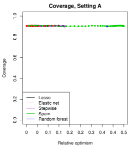
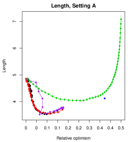
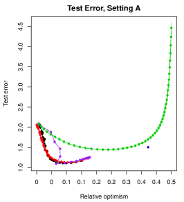
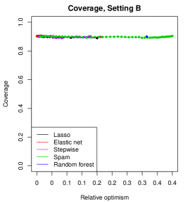
Figure 1: Comparison of conformal prediction intervals in low-dimensional problems with $n=200$, $d=20$, across a variety of base estimators.

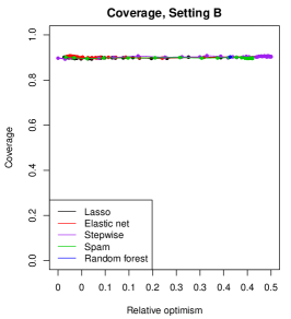
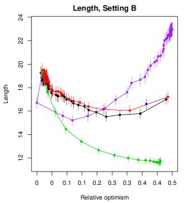
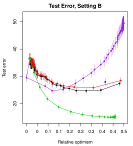
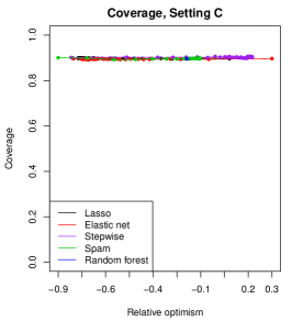
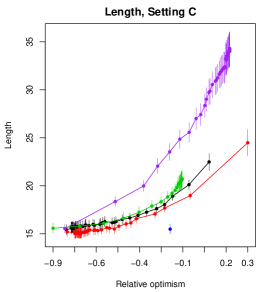
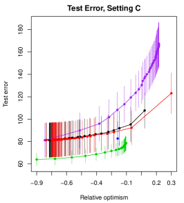
Figure 2: Comparison of conformal prediction intervals in high-dimensional problems with $n=200$, $d=2000$, across a variety of base estimators.

5 Extensions of Conformal Inference

The conformal and split conformal methods, combined with basically any fitting procedure in regression, provide finite-sample distribution-free predictive inferences. We describe some extensions of this framework to improve the interpretability and applicability of conformal inference.

5.1 In-Sample Split Conformal Inference

Given samples $(X_{i},Y_{i})$, $i=1,\ldots,n$, and a method that outputs a prediction band, we would often like to evaluate this band at some or all of the observed points $X_{i}$, $i=1,\ldots,n$. This is perhaps the most natural way to visualize any prediction band. However, the conformal prediction methods from Section 2 are designed to give a valid prediction interval at a future point $X_{n+1}$, from the same distribution as $\{X_{i},i=1,\ldots,n\}$, but not yet observed. If we apply the full or split conformal prediction methods at an observed feature value, then it is not easy to establish finite-sample validity of these methods.

A simple way to obtain valid in-sample predictive inference from the conformal methods is to treat each $X_{i}$ as a new feature value and use the other $n-1$ points as the original features (running either the full or split conformal methods on these $n-1$ points). This approach has two drawbacks. First, it seriously degrades the computational efficiency of the conformal methods—for full conformal, it multiplies the cost of the (already expensive) Algorithm 1 by $n$, making it perhaps intractable for even moderately large data sets; for split conformal, it multiplies the cost of Algorithm 2 by $n$, making it as expensive as the jackknife method in Algorithm 3. Second, if we denote by $C(X_{i})$ the prediction interval that results from this method at $X_{i}$, for $i=1,\ldots,n$, then one might expect the empirical coverage $\frac{1}{n}\sum_{i=1}^{n}\mathds{1}\{Y_{i}\in C(X_{i})\}$ to be at least $1-\alpha$, but this is not easy to show due to the complex dependence between the indicators.

Our proposed technique overcomes both of these drawbacks, and is a variant of the split conformal method that we call rank-one-out or ROO split conformal inference. The basic idea is quite similar to split conformal, but the ranking is conducted in a leave-one-out manner. The method is presented in Algorithm 4. For simplicity (as with our presentation of the split conformal method in Algorithm 2), we assume that $n$ is even, and only minor modifications are needed for $n$ odd. Computationally, ROO split conformal is very efficient. First, the fitting algorithm $\mathcal{A}$ (in the notation of Algorithm 4) only needs to be run twice. Second, for each split, the ranking of absolute residuals needs to be calculated just once; with careful updating, it can be reused in order to calculate the prediction interval for $X_{i}$ in $O(1)$ additional operations, for each $i=1,\ldots,n$.

Algorithm 4 Rank-One-Out Split Conformal

Input: Data $(X_{i},Y_{i})$, $i=1,\ldots,n$, miscoverage level $\alpha\in(0,1)$, regression algorithm $\mathcal{A}$

Output: Prediction intervals at each $X_{i}$, $i=1,\ldots,n$

Randomly split $\{1,\ldots,n\}$ into two equal-sized subsets $\mathcal{I}_{1}$, $\mathcal{I}_{2}$

for $k\in\{1,2\}$ do

     $\widehat{\mu}_{k}=\mathcal{A}\big{(}\{(X_{i},Y_{i}):i\in\mathcal{I}_{k}\}\big{)}$

     for $i\notin I_{k}$ do

         $R_{i}=|Y_{i}-\widehat{\mu}_{k}(X_{i})|$

     end for

     for $i\notin I_{k}$ do

         $d_{i}=$ the $m$th smallest value in $\{R_{j}:j\notin\mathcal{I}_{k},~{}j\neq i\}$, where $m=\lceil n/2(1-\alpha)\rceil$

         $C_{\mathrm{roo}}(X_{i})=[\widehat{\mu}_{k}(X_{i})-d_{i},\widehat{\mu}_{k}(X_{i})+d_{i}]$

     end for

end for

Return intervals $C_{\mathrm{roo}}(X_{i})$, $i=1,\ldots,n$

By symmetry in their construction, the ROO split conformal intervals have the in-sample finite-sample coverage property

$$\mathbb{P}\big{(}Y_{i}\in C_{\mathrm{roo}}(X_{i})\big{)}\geq 1-\alpha,\quad\text{for all $i=1,\ldots,n$}.$$

A practically interesting performance measure is the empirical in-sample average coverage $\frac{1}{n}\sum_{i=1}^{n}\mathds{1}\{Y_{i}\in C_{\mathrm{roo}}(X_{i})\}$. Our construction in Algorithm 4 indeed implies a weak dependence among the random indicators in this average, which leads to a slightly worse coverage guarantee for the empirical in-sample average coverage, with the difference from the nominal $1-\alpha$ level being of order $\sqrt{\log n/n}$, with high probability.

Theorem 5.1.

If $(X_{i},Y_{i})$, $i=1,\ldots,n$ are i.i.d., then for the ROO split conformal band $C_{\mathrm{roo}}$ constructed in Algorithm 4, there is an absolute constant $c>0$, such that for all $\epsilon>0$,

$$\mathbb{P}\bigg{(}\frac{1}{n}\sum_{i=1}^{n}\mathds{1}\{Y_{i}\in C_{\mathrm{roo}}(X_{i})\}\geq 1-\alpha-\epsilon\bigg{)}\geq 1-2\exp(-cn\epsilon^{2}).$$

Moreover, if we assume additionally that the residuals $R_{i}$, $i=1,\ldots,n$, have a continuous joint distribution, then for all $\epsilon>0$,

$$\mathbb{P}\bigg{(}1-\alpha-\epsilon\leq\frac{1}{n}\sum_{i=1}^{n}\mathds{1}\{Y_{i}\in C_{\mathrm{roo}}(X_{i})\}\leq 1-\alpha+\frac{2}{n}+\epsilon\bigg{)}\geq 1-2\exp(-cn\epsilon^{2}).$$

The proof of Theorem 5.1 uses McDiarmid’s inequality. It is conceptually straightforward but requires a careful tracking of dependencies and is deferred until Section A.3.

Remark 5.1.

An even simpler, and conservative approximation to each in-sample prediction interval $C_{\mathrm{roo}}(X_{i})$ is

$$\widetilde{C}_{\mathrm{roo}}(X_{i})=[\widehat{\mu}_{k}(X_{i})-\widetilde{d}_{k},\widehat{\mu}_{k}(X_{i})+\widetilde{d}_{k}],$$ (12)

where, using the notation of Algorithm 4, we define $\widetilde{d}_{k}$ to be the $m$th smallest element of the set $\{R_{i}:i\in\notin I_{k}\}$, for $m=\lceil(1-\alpha)n/2\rceil+1$. Therefore, now only a single sample quantile from the fitted residuals is needed for each split. As a price, each interval in (12) is wider than its counterpart from Algorithm 4 by at most one interquantile difference. Moreover, the results of Theorem 5.1 carry over to the prediction band $\widetilde{C}_{\mathrm{roo}}$: in the second probability statement (trapping the empirical in-sample average coverage from below and above), we need only change the $2/n$ term to $6/n$.

In Section A.1, we prove Theorem 2.3 as a modification of Theorem 5.1.

5.2 Locally-Weighted Conformal Inference

The full conformal and split conformal methods both tend to produce prediction bands $C(x)$ whose width is roughly constant over $x\in\mathbb{R}^{d}$. In fact, for split conformal, the width is exactly constant over $x$. For full conformal, the width can vary slightly as $x$ varies, but the difference is often negligible as long as the fitting method is moderately stable. This property—the width of $C(x)$ being roughly immune to $x$—is desirable if the spread of the residual $Y-\mu(X)$ does not vary substantially as $X$ varies. However, in some scenarios this will not be true, i.e., the residual variance will vary nontrivially with $X$, and in such a case we want the conformal band to adapt correspondingly.

We now introduce an extension to the conformal method that can account for nonconstant residual variance. Recall that, in order for the conformal inference method to have valid coverage, we can actually use any conformity score function to generalize the definition of (absolute) residuals as given in (8) of Remark 2.4. For the present extension, we modify the definition of residuals in Algorithm 1 by scaling the fitted residuals inversely by an estimated error spread. Formally

$$R_{y,i}=\frac{|Y_{i}-\widehat{\mu}_{y}(X_{i})|}{\widehat{\rho}_{y}(X_{i})},\;i=1,\ldots,n,\quad\text{and}\quad R_{y,n+1}=\frac{|y-\widehat{\mu}_{y}(x)|}{\widehat{\rho}_{y}(x)},$$ (13)

where now $\widehat{\rho}_{y}(x)$ denotes an estimate of the conditional mean absolute deviation (MAD) of $(Y-\mu(X))|X=x$, as a function of $x\in\mathbb{R}^{d}$. We choose to estimate the error spread by the mean absolute deviation of the fitted residual rather than the standard deviation, since the former exists in some cases in which the latter does not. Here, the conditional mean $\widehat{\mu}_{y}$ and conditional MAD $\widehat{\rho}_{y}$ can either be estimated jointly, or more simply, the conditional mean $\widehat{\mu}_{y}$ can be estimated first, and then the conditional MAD $\widehat{\rho}_{y}$ can be estimated using the collection of fitted absolute residuals $|Y_{i}-\widehat{\mu}_{y}(X_{i})|$, $i=1,\ldots,n$ and $|y-\widehat{\mu}_{y}(X_{n+1})|$. With the locally-weighted residuals in (13), the validity and accuracy properties of the full conformal inference method carry over.

For the split conformal and the ROO split conformal methods, the extension is similar. In Algorithm 2, we instead use locally-weighted residuals

$$R_{i}=\frac{|Y_{i}-\widehat{\mu}(X_{i})|}{\widehat{\rho}(X_{i})},\;i\in\mathcal{I}_{2},$$ (14)

where the conditional mean $\widehat{\mu}$ and conditional MAD $\widehat{\rho}$ are fit on the samples in $\mathcal{I}_{1}$, either jointly or in a two-step fashion, as explained above. The output prediction interval at a point $x$ must also be modified, now being $[\widehat{\mu}(x)-\widehat{\rho}(x)d,\;\widehat{\mu}(x)+\widehat{\rho}(x)d]$. In Algorithm 4, analogous modifications are performed. Using locally-weighted residuals, as in (14), the validity and accuracy properties of the split methods, both finite sample and asymptotic, in Theorems 2.2, 2.3 and 5.1, again carry over. The jackknife interval can also be extended in a similar fashion.

Figure 3 displays a simple example of the split conformal method using locally-weighted residuals. We let $n=1000$, drew i.i.d. copies $X_{i}\sim\mathrm{Unif}(0,2\pi)$, $i=1,\ldots,n$, and let

$$Y_{i}=\sin(X_{i})+\frac{\pi|X_{i}|}{20}\epsilon_{i},\;i=1,\ldots,n,$$

for i.i.d. copies $\epsilon_{i}\sim N(0,1)$, $i=1,\ldots,n$. We divided the data set randomly into two halves $\mathcal{I}_{1},\mathcal{I}_{2}$, and fit the conditional mean estimator $\widehat{\mu}$ on the samples from the first half $\mathcal{I}_{1}$ using a smoothing spline, whose tuning parameter was chosen by cross-validation. This was then used to produce a 90% prediction band, according to the usual (unweighted) split conformal strategy, that has constant width by design; it is plotted, as a function of $x\in\mathbb{R}$, in the top left panel of Figure 3. For our locally-weighted version, we then fit a conditional MAD estimator $\widehat{\rho}$ on $|Y_{i}-\widehat{\mu}(X_{i})|$, $i\in\mathcal{I}_{1}$, again using a smoothing spline, whose tuning parameter was chosen by cross-validation. Locally-weighted residuals were used to produce a 90% prediction band, with locally-varying width, plotted in the top right panel of the figure. Visually, the locally-weighted band adapts better to the heteroskedastic nature of the data. This is confirmed by looking at the length of the locally-weighted band as a function of $x$ in the bottom right panel. It is also supported by the improved empirical average length offered by the locally-weighted prediction band, computed over 5000 new draws from $\mathrm{Unif}(0,2\pi)$, which is 1.105 versus 1.247 for the unweighted band. In terms of average coverage, again computed empirically over the same 5000 new draws, both methods are very close to the nominal 90% level, with the unweighted version at 89.7% and the weighted version at 89.9%. Most importantly, the locally-weighted version does a better job here of maintaining a conditional coverage level of around 90% across all $x$, as shown in the bottom left panel, as compared to the unweighted split conformal method, which over-covers for smaller $x$ and under-covers for larger $x$.

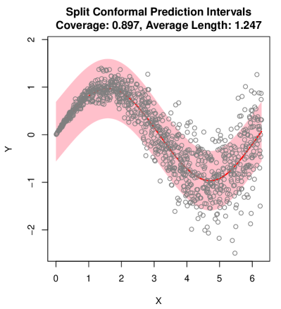
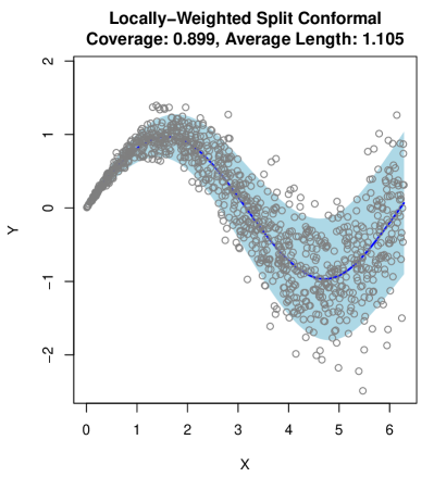
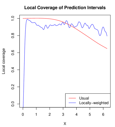
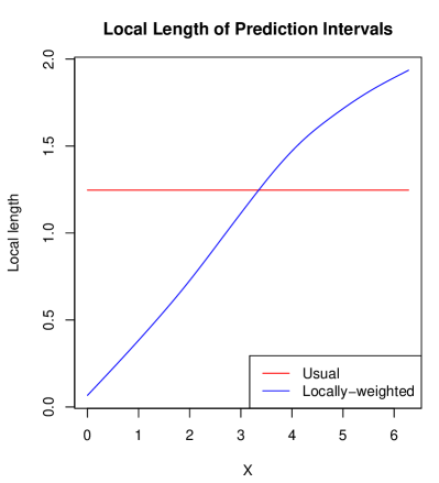
Figure 3: A simple univariate example of the usual (unweighted) split conformal and locally-weighted split conformal prediction bands. The top left panel shows the split conformal band, and the top right shows the locally-weighted split conformal band; we can see that the latter properly adapts to the heteroskedastic nature of the data, whereas the former has constant length over all $x$ (by construction). The bottom left and right panels plot the empirical local coverage and local length measures (which have been mildly smoothed as functions of $x$ for visibility). The locally-weighted split conformal method maintains a roughly constant level of local coverage across $x$, but its band has a varying local length; the usual split conformal method exhibits precisely the opposite trends.

Lastly, it is worth remarking that if the noise is indeed homoskedastic, then of course using such a locally-weighted conformal band will have generally a inflated (average) length compared to the usual unweighted conformal band, due to the additional randomness in estimating the conditional MAD. In Appendix B, we mimic the setup in Figure 3 but with homoskedastic noise to demonstrate that, in this particular problem, there is not too much inflation in the length of the locally-weighted band compared to the usual band.

6 Model-Free Variable Importance: LOCO

In this section, we discuss the problem of estimating the importance of each variable in a prediction model. A critical question is: how do we assess variable importance when we are treating the working model as incorrect? One possibility, if we are fitting a linear model with variable selection, is to interpret the coefficients as estimates of the parameters in the best linear approximation to the mean function $\mu$. This has been studied in, e.g., Wasserman (2014); Buja et al. (2014); Tibshirani et al. (2016). However, we take a different approach for two reasons. First, our method is not limited to linear regression. Second, the spirit of our approach is to focus on predictive quantities and we want to measure variable importance directly in terms of prediction. Our approach is similar in spirit to the variable importance measure used in random forests (Breiman, 2001).

Our proposal, leave-one-covariate-out or LOCO inference, proceeds as follows. Denote by $\widehat{\mu}$ our estimate of the mean function, fit on data $(X_{i},Y_{i})$, $i\in\mathcal{I}_{1}$ for some $\mathcal{I}_{1}\subseteq\{1,\ldots,n\}$. To investigate the importance of the $j$th covariate, we refit our estimate of the mean function on the data set $(X_{i}(-j),Y_{i})$, $i\in\mathcal{I}_{1}$, where in each $X_{i}(-j)=(X_{i}(1),\ldots,X_{i}(j-1),X_{i}(j+1),\ldots,X_{i}(d))\in\mathbb{R}^{d-1}$, we have removed the $j$th covariate. Denote by $\widehat{\mu}_{(-j)}$ this refitted mean function, and denote the excess prediction error of covariate $j$, at a new i.i.d. draw $(X_{n+1},Y_{n+1})$, by

$$\Delta_{j}(X_{n+1},Y_{n+1})=|Y_{n+1}-\widehat{\mu}_{(-j)}(X_{n+1})|-|Y_{n+1}-\widehat{\mu}(X_{n+1})|.$$

The random variable $\Delta_{j}(X_{n+1},Y_{n+1})$ measures the increase in prediction error due to not having access to covariate $j$ in our data set, and will be the basis for inferential statements about variable importance. There are two ways to look at $\Delta_{j}(X_{n+1},Y_{n+1})$, as discussed below.

6.1 Local Measure of Variable Importance

Using conformal prediction bands, we can construct a valid prediction interval for the random variable $\Delta_{j}(X_{n+1},Y_{n+1})$, as follows. Let $C$ denote a conformal prediction set for $Y_{n+1}$ given $X_{n+1}$, having coverage $1-\alpha$, constructed from either the full or split methods—in the former, the index set used for the fitting of $\widehat{\mu}$ and $\widehat{\mu}_{(-j)}$ is $\mathcal{I}_{1}=\{1,\ldots,n\}$, and in the latter, it is $\mathcal{I}_{1}\subsetneq\{1,\ldots,n\}$, a proper subset (its complement $\mathcal{I}_{2}$ is used for computing the appropriate sample quantile of residuals). Now define

$$W_{j}(x)=\left\{|y-\widehat{\mu}_{(-j)}(x)|-|y-\widehat{\mu}(x)|\;:\;y\in C(x)\right\}.$$

From the finite-sample validity of $C$, we immediately have

$$\mathbb{P}\big{(}\Delta_{j}(X_{n+1},Y_{n+1})\in W_{j}(X_{n+1}),\;\text{for all $j=1,\ldots,d$}\big{)}\geq 1-\alpha.$$ (15)

It is important to emphasize that the prediction sets $W_{1},\ldots,W_{d}$ are valid in finite-sample, without distributional assumptions. Furthermore, they are uniformly valid over $j$, and there is no need to do any multiplicity adjustment. One can decide to construct $W_{j}(X_{n+1})$ at a single fixed $j$, at all $j=1,\ldots,d$, or at a randomly chosen $j$ (say, the result of a variable selection procedure on the given data $(X_{i},Y_{i})$, $i=1,\ldots,n$), and in each case the interval(s) will have proper coverage.

As with the guarantees from conformal inference, the coverage statement (15) is marginal over $X_{n+1}$, and in general, does not hold conditionally at $X_{n+1}=x$. But, to summarize the effect of covariate $j$, we can still plot the intervals $W_{j}(X_{i})$ for $i=1,\ldots,n$, and loosely interpret these as making local statements about variable importance.

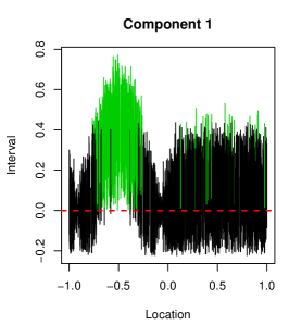
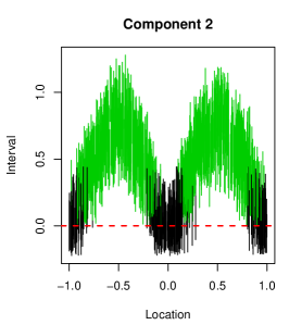
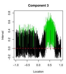
Figure 4: In-sample prediction intervals for $\Delta_{j}(X_{i})$ across all covariates $j=1,\ldots,6$ and samples $i=1,\ldots,1000$, in an additive model setting described in the text. Each interval that lies strictly above zero is colored in green.

We illustrate this idea in a low-dimensional additive model, where $d=6$ and the mean function is $\mu(x)=\sum_{j=1}^{6}f_{j}(x(j))$, with $f_{1}(t)=\sin(\pi(1+t))\mathds{1}\{t<0\}$, $f_{2}(t)=\sin(\pi t)$, $f_{3}(t)=\sin(\pi(1+t))\mathds{1}\{t>0\}$, and $f_{4}=f_{5}=f_{6}=0$. We generated $n=1000$ i.i.d pairs $(X_{i},Y_{i})$, $i=1,\ldots,1000$, where each $X_{i}\sim\mathrm{Unif}[-1,1]^{d}$ and $Y_{i}=\mu(X_{i})+\epsilon_{i}$ for $\epsilon_{i}\sim N(0,1)$. We then computed each interval $W_{j}(X_{i})$ using the ROO split conformal technique at the miscoverage level $\alpha=0.1$, using an additive model as the base estimator (each component modeled by a spline with 5 degrees of freedom). The intervals are plotted in Figure 4. We can see that many intervals for components $j=1,2,3$ lie strictly above zero, indicating that leaving out such covariates is damaging to the predictive accuracy of the estimator. Furthermore, the locations at which these intervals lie above zero are precisely locations at which the underlying components $f_{1},f_{2},f_{3}$ deviate significantly from zero. On the other hand, the intervals for components $j=4,5,6$ all contain zero, as expected.

6.2 Global Measures of Variable Importance

For a more global measure of variable importance, we can focus on the distribution of $\Delta_{j}(X_{n+1},Y_{n+1})$, marginally over $(X_{n+1},Y_{n+1})$. We rely on a splitting approach, where the index set used for the training of $\widehat{\mu}$ and $\widehat{\mu}_{(-j)}$ is $\mathcal{I}_{1}\subsetneq\{1,\ldots,n\}$, a proper subset. Denote by $\mathcal{I}_{2}$ its complement, and by $\mathcal{D}_{k}=\{(X_{i},Y_{i}):i\in\mathcal{I}_{k}\}$, $k=1,2$ the data samples in each index set. Define

$$G_{j}(t)=\mathbb{P}\Big{(}\Delta_{j}(X_{n+1},Y_{n+1})\leq t\;\big{|}\;\mathcal{D}_{1}\Big{)},\;t\in\mathbb{R},$$

the distribution function of $\Delta_{j}(X_{n+1},Y_{n+1})$ conditional on the data $\mathcal{D}_{1}$ in the first half of the data-split. We will now infer parameters of $G_{j}$ such as its mean $\theta_{j}$ or median $m_{j}$. For the former parameter,

$$\theta_{j}=\mathbb{E}\Big{[}\Delta_{j}(X_{n+1},Y_{n+1})\;\big{|}\;\mathcal{D}_{1}\Big{]},$$

we can obtain the asymptotic $1-\alpha$ confidence interval

$$\bigg{[}\widehat{\theta}_{j}-\frac{z_{\alpha/2}s_{j}}{\sqrt{n/2}},\;\widehat{\theta}_{j}+\frac{z_{\alpha/2}s_{j}}{\sqrt{n/2}}\bigg{]},$$

where $\widehat{\theta}_{j}=(n/2)^{-1}\sum_{i\in\mathcal{I}_{2}}\Delta_{j}(X_{i},Y_{i})$ is the sample mean, $s_{j}^{2}$ is the analogous sample variance, measured on $\mathcal{D}_{2}$, and $z_{\alpha/2}$ is the $1-\alpha/2$ quantile of the standard normal distribution. Similarly, we can perform a one-sided hypothesis test of

$$H_{0}:\theta_{j}\leq 0\quad\text{versus}\quad H_{1}:\theta_{j}>0$$

by rejecting when $\sqrt{n/2}\cdot\widehat{\theta}_{j}/s_{j}>z_{\alpha}$. Although these inferences are asymptotic, the convergence to its asymptotic limit is uniform (say, as governed by the Berry-Esseen Theorem) and independent of the feature dimension $d$ (since $\Delta_{j}(X_{n+1},Y_{n+1})$ is always univariate). To control for multiplicity, we suggest replacing $\alpha$ in the above with $\alpha/|S|$ where $S$ is the set of variables whose importance is to be tested.

Inference for the parameter $\theta_{j}$ requires existence of the first and second moments for the error term. In practice it may be more stable to consider the median parameter

$$m_{j}=\mathrm{median}\Big{[}\Delta_{j}(X_{n+1},Y_{n+1})\;\big{|}\;\mathcal{D}_{1}\Big{]}.$$

We can conduct nonasymptotic inferences about $m_{j}$ using standard, nonparametric tests such as the sign test or the Wilcoxon signed-rank test, applied to $\Delta_{j}(X_{i},Y_{i})$, $i\in\mathcal{I}_{2}$. This allows us to test

$$H_{0}:m_{j}\leq 0\quad\text{versus}\quad H_{1}:m_{j}>0$$

with finite-sample validity under essentially no assumptions on the distribution $G_{j}$ (the sign test only requires continuity, and the Wilcoxon test requires continuity and symmetry). Confidence intervals for $m_{j}$ can be obtained by inverting the (two-sided) versions of the sign and Wilcoxon tests, as well. Again, we suggest replacing $\alpha$ with $\alpha/|S|$ to adjust for multiplicity, where $S$ is the set of variables to be tested.

We finish with an example of a high-dimensional linear regression problem with $n=200$ observations and $d=500$ variables. The mean function $\mu(x)$ was defined to be a linear function of $x(1),\ldots,x(5)$ only, with coefficients drawn i.i.d. from $N(0,4)$. We drew $X_{i}(j)\sim N(0,1)$ independently across all $i=1,\ldots,200$ and $j=1,\ldots,500$, and then defined the responses by $Y_{i}=\mu(X_{i})+\epsilon_{i}$, for $\epsilon_{i}\sim N(0,1)$, $i=1,\ldots,200$. A single data-split was applied, and the on the first half we fit the lasso estimator $\widehat{\mu}$ with the tuning parameter $\lambda$ chosen by 10-fold cross-validation. The set of active predictors $S$ was collected, which had size $|S|=17$; the set $S$ included the 5 truly relevant variables, but also 12 irrelevant ones. We then refit the lasso estimator $\widehat{\mu}_{(-j)}$ using the same cross-validation, with covariate $j$ excluded, for each $j\in S$. On the second half of the data, we applied the Wilcoxon rank sum test to compute confidence intervals for the median excess test error due to variable dropping, $m_{j}$, for each $j\in S$. These intervals were properly corrected for multiplicity: each was computed at the level $1-0.1/17$ in order to obtain a simultaneous level $1-0.1=0.9$ of coverage. Figure 5 shows the results. We can see that the intervals for the first 5 variables are well above zero, and those for the next 12 all hover around zero, as desired.

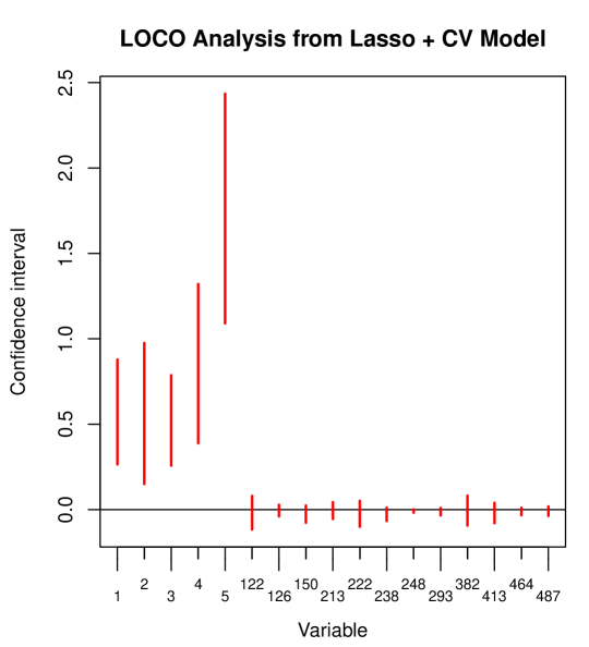
Figure 5: Wilcoxon-based confidence intervals for the median excess test error due to variable dropping, for all selected variables in a high-dimensional linear regression example with $n=200$ and $d=500$ described in the text.

The problem of inference after model selection is an important but also subtle topic and we are only dealing with the issue briefly here. In a future paper we will thoroughly compare several approaches including LOCO.

7 Conclusion

Current high-dimensional inference methods make strong assumptions while little is known about their robustness against model misspecification. We have shown that if we focus on prediction bands, almost all existing point estimators can be used to build valid prediction bands, even when the model is grossly misspecified, as long as the data are i.i.d. Conformal inference is similar to the jackknife, bootstrap, and cross-validation in the use of symmetry of data. A remarkable difference in conformal inference is its “out-of-sample fitting”. That is, unlike most existing prediction methods which fit a model using the training sample and then apply the fitted model to any new data points for prediction, the full conformal method refits the model each time when a new prediction is requested at a new value $X_{n+1}$. An important and distinct consequence of such an “out-of-sample fitting” is the guaranteed finite-sample coverage property.

The distribution-free coverage offered by conformal intervals is marginal. The conditional coverage may be larger than $1-\alpha$ at some values of $X_{n+1}=x$ and smaller than $1-\alpha$ at other values. This should not be viewed as a disadvantage of conformal inference, as the statistical accuracy of the conformal prediction band is strongly tied to the base estimator. In a sense, conformal inference broadens the scope and value of any regression estimator at nearly no cost: if the estimator is accurate (which usually requires an approximately correctly specified model, and a proper choice of tuning parameter), then the conformal prediction band is near-optimal; if the estimator is bad, then we still have valid marginal coverage. As a result, it makes sense to use a conformal prediction band as a diagnostic and comparison tool for regression function estimators.

There are many directions in conformal inference that are worth exploring. Here we give a short list. First, it would be interesting to better understand the trade-off between the full and split conformal methods. The split conformal method is fast, but at the cost of less accurate inference. Also, in practice it would be desirable to reduce the additional randomness caused by splitting the data. In this paper we showed that aggregating results from multiple splits (using a Bonferonni-type correction) leads to wider bands. It would be practically appealing to develop novel methods that more efficiently combine results from multiple splits. Second, it would be interesting to see how conformal inference can help with model-free variable selection. Our leave-one-covariate-out (LOCO) method is a first step in this direction. However, the current version of LOCO based on excess prediction error can only be implemented with the split conformal method due to computational reasons. When split conformal is used, the inference is then conditional on the model fitted in the first half of the data. The effect of random splitting inevitably raises an issue of selective inference, which needs to be appropriately addressed. In a future paper, we will report on detailed comparisons of LOCO with other approaches to high-dimensional inference.

Appendix A Technical Proofs

A.1 Proofs for Section 2

Proof of Theorem 2.1.

The first part (the lower bound) comes directly from the definition of the conformal interval in (7), and the (discrete) p-value property in (6). We focus on the second part (upper bound). Define $\alpha^{\prime}=\alpha-1/(n+1)$. By assuming a continuous joint distribution of the fitted residuals, we know that the values $R_{y,1},\ldots,R_{y,n+1}$ are all distinct with probability one. The set $C_{\mathrm{conf}}$ in (7) is equivalent to the set of all points $y$ such that $R_{y,n+1}$ ranks among the $\lceil(n+1)(1-\alpha)\rceil$ smallest of all $R_{y,1},\ldots,R_{y,n+1}$. Consider now the set $D(X_{n+1})$ consisting of points $y$ such that $R_{y,n+1}$ is among the $\lceil(n+1)\alpha^{\prime}\rceil$ largest. Then by construction

$$\mathbb{P}\big{(}Y_{n+1}\in D(X_{n+1})\big{)}\geq\alpha^{\prime},$$

and yet $C_{\mathrm{conf}}(X_{n+1})\cap D(X_{n+1})=\emptyset$, which implies the result. ∎

Proof of Theorem 2.2.

The first part (lower bound) follows directly by symmetry between the residual at $(X_{n+1},Y_{n+1})$ and those at $(X_{i},Y_{i})$, $i\in\mathcal{I}_{2}$. We prove the upper bound in the second part. Assuming a continuous joint distribution of residual, and hence no ties, the set $C_{\mathrm{split}}(X_{n+1})$ excludes the values of $y$ such that $|y-\widehat{\mu}(X_{n+1})|$ is among the $(n/2)-\lceil(n/2+1)(1-\alpha)\rceil$ largest in $\{R_{i}:i\in\mathcal{I}_{2}\}$. Denote the set of these excluded points as $D(X_{n+1})$. Then again by symmetry,

$$\mathbb{P}\big{(}Y_{n+1}\in D(X_{n+1})\big{)}\geq\frac{(n/2)-\lceil(n/2+1)(1-\alpha)\rceil}{n/2+1}\geq\alpha-2/(n+2),$$

which completes the proof. ∎

Proof of Theorem 2.4.

Without loss of generality, we assume that the sample size is $2n$. The individual split conformal interval has length infinity if $\alpha/N<1/n$. Therefore, we only need to consider $2\leq N\leq\alpha n\leq n$. Also, in this proof we will ignore all rounding issues by directly working with the empirical quantiles. The differences caused by rounding are negligible.

For $j=1,\ldots,N$, the $j$th split conformal prediction band at $X$, $C_{{\rm split},j}(X)$, is an interval with half-width $\widehat{F}^{-1}_{n,j}(1-\alpha/N)$, where $\widehat{F}_{n,j}$ is the empirical CDF of fitted absolute residuals in the ranking subsample in the $j$th split.

We focus on the event

$$\left\{\max_{j=1,\ldots,N}\|\widehat{\mu}_{j}-\widetilde{\mu}\|_{\infty}<\eta_{n}\right\},$$

which has probability at least $1-N\rho_{n}\geq 1-n\rho_{n}\rightarrow 1$. On this event, the length of $C^{(N)}_{\rm split}(X)$ is at least

$$2\min_{j=1,\ldots,N}\widetilde{F}_{n,j}^{-1}(1-\alpha/N)-2\eta_{n},$$

where $\widetilde{F}_{n,j}$ is the empirical CDF of the absolute residuals about $\widetilde{\mu}$ in the ranking subsample in the $j$th split.

Note that the split conformal band $C_{{\rm split},1}(X)$ from a single split has length no more than $2\widetilde{F}_{n,1}^{-1}(1-\alpha)+2\eta_{n}$ on the event we focus on. Therefore, it suffices to show that

$$\mathbb{P}\left(\widetilde{F}_{n,1}^{-1}(1-\alpha)<\widetilde{F}^{-1}_{n,j}(1-\alpha/N)-2\eta_{n},\;j=1,\ldots,N\right)\rightarrow 1.$$ (16)

Let $\widetilde{F}$ be the CDF of $|Y-\widetilde{\mu}(X)|$. Note that it is $\widetilde{F}_{n,j}$, instead of $\widehat{F}_{n,j}$, that corresponds to $\widetilde{F}$. By the Dvoretzky-Kiefer-Wolfowitz inequality, we have

$$\mathbb{P}\left(\widetilde{F}^{-1}_{n,j}(1-\alpha/N)\leq\widetilde{F}^{-1}(1-\alpha/1.6)\right) \leq\mathbb{P}\left(\|\widetilde{F}_{n,j}-\widetilde{F}\|_{\infty}\geq\alpha(1/1.6-1/N)\right)$$

$$\leq\mathbb{P}\left(\|\widetilde{F}_{n,j}-\widetilde{F}\|_{\infty}\geq\alpha/8\right)$$

$$\leq 2\exp(-n\alpha^{2}/32).$$

Using a union bound,

$$\mathbb{P}\left(\min_{j=1,\ldots,N}\widetilde{F}_{n,j}^{-1}(1-\alpha/N)\leq\widetilde{F}^{-1}(1-\alpha/1.6)\right)\leq 2N\exp(-n\alpha^{2}/32).$$

On the other hand,

$$\mathbb{P}\left(\widetilde{F}_{n,1}^{-1}(1-\alpha)\geq\widetilde{F}^{-1}(1-\alpha/1.4)\right) \leq\mathbb{P}\left(\|\widetilde{F}_{n,1}-\widetilde{F}\|_{\infty}\geq\alpha(1-1/1.4)\right)\leq 2\exp(-n\alpha^{2}/8).$$

So with probability at least $1-2\exp(-n\alpha^{2}/8)-2N\exp(-n\alpha^{2}/32)$ we have

$$\min_{j=1,\ldots,N}\widetilde{F}_{n,j}^{-1}(1-\alpha/N)-\widetilde{F}_{n,1}^{-1}(1-\alpha)\geq\widetilde{F}^{-1}(1-\alpha/1.6)-\widetilde{F}^{-1}(1-\alpha/1.4)>0.$$

Therefore we conclude (16), as $\eta_{n}=o(1)$. ∎

Proof of Theorem 2.3.

Comparing the close similarity of $\widetilde{d}_{1}$ in (12) and $d$ in Algorithm 2, we see that $\widetilde{d}_{1}=d$ if we choose the target coverage levels to be $1-\alpha$ for the regular split conformal band $C_{\mathrm{split}}$, and $1-(\alpha+2\alpha/n)$ for the modified ROO split conformal band $\widetilde{C}_{\mathrm{roo}}$. The desired result follows immediately by replacing $\alpha$ by $\alpha+2\alpha/n$ in Theorem 5.1, as it applies to $\widetilde{C}_{\mathrm{roo}}$ (explained in the above remark). ∎

A.2 Proofs for Section 3

Proof of Theorem 3.1.

For any $t>0$, by Fubini’s theorem and independence between $\epsilon$ and $(\Delta_{n},X)$,

$$F_{n}(t) =\mathbb{P}(|Y-\widehat{\mu}_{n}(X)|\leq t)$$

$$=\mathbb{P}(-t+\Delta_{n}(X)\leq\epsilon\leq t+\Delta_{n}(X))$$

$$=\mathbb{E}_{\widehat{\mu}_{n},X}[F_{0}(t+\Delta_{n}(X))-F_{0}(-t+\Delta_{n}(X))],$$ (17)

where $F_{0}$ is the CDF of $\epsilon$.

Let $f_{0}$ be the density function of $F_{0}$. We can approximate $F_{0}$ at any $t$ using first order Taylor expansion

$$F_{0}(t+\delta)=F_{0}(t)+\delta f_{0}(t)+\delta^{2}R(t,\delta),$$

where $R(t,\delta)=0.5\int_{0}^{1}(1-u)f^{\prime}_{0}(t+u\delta)du$ satisfies $\sup_{t,\delta}|R(t,\delta)|\leq M/4$.

Next, using symmetry of $F_{0}$ we have $f_{0}(t)=f_{0}(-t)$ for all $t$, the RHS of (17) becomes

$$\mathbb{E}_{\widehat{\mu}_{n},X}[ F_{0}(t+\Delta_{n}(X))-F_{0}(-t+\Delta_{n}(X))]$$

$$=\mathbb{E}_{\widehat{\mu}_{n},X}[F_{0}(t)+\Delta_{n}(X)f_{0}(t)+\Delta_{n}^{2}(X)R(t,\Delta_{n}(X))$$

$$\qquad\qquad-F_{0}(-t)-\Delta_{n}(X)f_{0}(-t)-\Delta_{n}^{2}(X)R(-t,\Delta_{n}(X))]$$

$$=F_{0}(t)-F_{0}(-t)+\mathbb{E}_{\widehat{\mu}_{n},X}[\Delta_{n}^{2}(X)W]$$

$$=F(t)+\mathbb{E}_{\widehat{\mu}_{n},X}[\Delta_{n}^{2}(X)W],$$

where $W=R(t,\Delta_{n}(X))-R(-t,\Delta_{n}(X))$. Equation (10) follows immediately since $|W|\leq M/2$, almost surely.

Next we show equation (11). Because $F$ has density at least $r>0$ in an open neighborhood of $q_{\alpha}$, if $t<q_{\alpha}-\delta$ for some $\delta>(M/2r)\mathbb{E}(\Delta_{n}^{2}(X))$ then

$$F_{n}(t)\leq F(q_{\alpha}-\delta)+(M/2)\mathbb{E}(\Delta_{n}^{2}(X))$$

$$\leq F(q_{\alpha})-\delta r+(M/2)\mathbb{E}(\Delta_{n}^{2}(X))$$

$$<1-\alpha.$$

Thus $q_{n,\alpha}\geq q_{\alpha}-(M/2r)\mathbb{E}\Delta_{n}^{2}(X)$. Similarly we can show that $q_{n,\alpha}\leq q_{\alpha}+(M/2r)\mathbb{E}\Delta_{n}^{2}(X)$, and hence establish the claimed result. ∎

Proof of Theorem 3.2.

Without a loss of generality, we assume that the split conformal band is obtained using $2n$ samples. Let $\widetilde{q}_{\alpha}$ be the $\alpha$ upper quantile of $|Y-\widetilde{\mu}(X)|$. We first show that

$$|\widetilde{q}_{\alpha}-q_{n,\alpha}|\leq\rho_{n}/r+\eta_{n},$$ (18)

where $r>0$ is the assumed lower bound on $\widetilde{f}$ in an open neighborhood of its $\alpha$ upper quantile. To see this, note that

$$\mathbb{P}(|Y-\widehat{\mu}_{n}(X)|\leq\widetilde{q}_{\alpha+\rho_{n}}-\eta_{n}) \leq\mathbb{P}\Big{(}|Y-\widehat{\mu}_{n}(X)|\leq\widetilde{q}_{\alpha+\rho_{n}}-\eta_{n},\;\|\widetilde{\mu}-\widehat{\mu}_{n}\|_{\infty}\leq\eta_{n}\Big{)}+\rho_{n}$$

$$\leq\mathbb{P}(|Y-\widetilde{\mu}(X)|\leq\widetilde{q}_{\alpha+\rho_{n}})+\rho_{n}$$

$$=1-\alpha-\rho_{n}+\rho_{n}=1-\alpha.$$

Thus $q_{n,\alpha}\geq\widetilde{q}_{\alpha+\rho_{n}}-\eta_{n}\geq\widetilde{q}_{\alpha}-\rho_{n}/r-\eta_{n}$. Similarly, $q_{n,\alpha}\leq\widetilde{q}_{\alpha-\rho_{n}}+\eta_{n}\leq\widetilde{q}_{\alpha}+\rho_{n}/r+\eta_{n}$.

The width of split conformal band is $2\widehat{F}_{n}^{-1}(1-\alpha)$, where $\widehat{F}_{n}$ denotes the empirical CDF of $|Y_{i}-\widehat{\mu}_{n}(X_{i})|$, $i=1,\ldots,n$, and $\widehat{\mu}_{n}=\mathcal{A}_{n}(\{(X_{i},Y_{i}):i=n+1,\ldots,2n\})$. On the event $\{\|\widehat{\mu}_{n}-\widetilde{\mu}\|_{\infty}\leq\eta_{n}\}$, we have $|Y_{i}-\widehat{\mu}_{n}(X_{i})|-|Y_{i}-\widetilde{\mu}(X_{i})|\leq\eta_{n}$ for $1=1,\ldots,n$. Therefore, denoting by $\widetilde{F}_{n}$ the empirical CDF of $|Y_{i}-\widetilde{\mu}(X_{i})|$, $i=1,\ldots,n$, we have

$$\mathbb{P}\left(|\widehat{F}_{n}^{-1}(1-\alpha)-\widetilde{F}_{n}^{-1}(1-\alpha)|\leq\eta_{n}\right)\geq 1-\rho_{n}.$$ (19)

Using standard empirical quantile theory for i.i.d. data and using the assumption that $\widetilde{f}$ is bounded from below by $r>0$ in a neighborhood of its $\alpha$ upper quantile, we have

$$\widetilde{F}_{n}^{-1}(1-\alpha)=\widetilde{q}_{\alpha}+O_{\mathbb{P}}(n^{-1/2}).$$ (20)

Combining (18), (19), and (20), we conclude that

$$|\widehat{F}_{n}^{-1}(1-\alpha)-q_{n,\alpha}|=O_{\mathbb{P}}(\eta_{n}+\rho_{n}+n^{-1/2}),$$

which gives the result. ∎

Proof of Theorem 3.3.

We focus on the event

$$\{\|\widehat{\mu}_{n}-\widetilde{\mu}\|_{\infty}\leq\eta_{n}\}\cap\left\{\sup_{y\in\mathcal{Y}}\|\widehat{\mu}_{n}-\widehat{\mu}_{n,(X,y)}\|_{\infty}\leq\eta_{n}\right\},$$

which, by assumption, has probability at least $1-2\rho_{n}\rightarrow 1$. On this event, we have

$$\Big{|}|Y_{i}-\widehat{\mu}_{n,(X,y)}(X_{i})|-|Y_{i}-\widetilde{\mu}(X_{i})|\Big{|}\leq 2\eta_{n},\quad i=1,\ldots,n,$$ (21)

$$\Big{|}|y-\widehat{\mu}_{n,(X,y)}(X)|-|y-\widetilde{\mu}(X)|\Big{|}\leq 2\eta_{n}.$$ (22)

With (21) and (22), by the construction of full conformal prediction interval we can directly verify the following two facts.

1. $y\in C_{n,{\rm conf}}(X)$ if $|y-\widetilde{\mu}(X)|\leq\widetilde{F}_{n}^{-1}(1-\alpha)-4\eta_{n}$, and

2. $y\notin C_{n,{\rm conf}}(X)$ if $|y-\widetilde{\mu}(X)|\geq\widetilde{F}_{n}^{-1}(1-(\alpha-3/n))+4\eta_{n}$,

where $\widetilde{F}_{n}$ is the empirical CDF of $|Y_{i}-\widetilde{\mu}(X_{i})|$, $i=1,\ldots,n$.

Therefore, the length of $C_{n,{\rm conf}}(X)$ satisfies

$$\nu_{n,{\rm conf}}(X)=2\widetilde{q}_{\alpha}+O_{\mathbb{P}}(\eta_{n}+n^{-1/2}).$$

The claimed result follows by further combining the above equation with (18). ∎

Proof of Theorem 3.4.

Without loss of generality, we assume that the split conformal band is obtained using $2n$ data points. The proof consists of two steps. First we establish that $\widehat{\mu}_{n}(X)-\mu(X)=o_{\mathbb{P}}(1)$. Second we establish that $\widehat{F}_{n}^{-1}(1-\alpha)-q_{\alpha}=o_{\mathbb{P}}(1)$, where $\widehat{F}_{n}$ is the empirical CDF of $|Y_{i}-\widehat{\mu}_{n}(X_{i})|$, $i=1,\ldots,n$, and $\widehat{\mu}_{n}=\mathcal{A}_{n}(\{(X_{i},Y_{i}):i=n+1,\ldots,2n\})$.

We now show the first part. We will focus on the event that $\{\mathbb{E}_{X}(\widehat{\mu}_{n}(X)-\mu(X))^{2}\leq\eta_{n}\}$, which has probability at least $1-\rho_{n}$ by Assumption A4. On this event, applying Markov’s inequality, we have that $\mathbb{P}(X\in B_{n}^{c}\,|\,\widehat{\mu}_{n})\geq 1-\eta_{n}^{1/3}$, where $B_{n}=\{x:|\widehat{\mu}_{n}(x)-\mu(x)|\geq\eta_{n}^{1/3}\}$. Hence we conclude that $\mathbb{P}_{X,\widehat{\mu}_{n}}(|\widehat{\mu}_{n}(X)-\mu(X)|\geq\eta_{n}^{1/3})\leq\eta_{n}^{1/3}+\rho_{n}\rightarrow 0$ as $n\rightarrow\infty$, and the first part of the proof is complete.

For the second part, define $\mathcal{I}_{1}=\{i\in\{1,\ldots,n\}:X_{i}\in B_{n}^{c}\}$ and $\mathcal{I}_{2}=\{1,\ldots,n\}\backslash\mathcal{I}_{1}$. Note that $B_{n}$ is independent of $(X_{i},Y_{i})$, $i=1,\ldots,n$. Using Hoeffding’s inequality conditionally on $\widehat{\mu}_{n}$, we have $|\mathcal{I}_{2}|\leq n\eta_{n}^{1/3}+c\sqrt{n\log n}=o(n)$ with probability tending to 1, for some absolute constant $c>0$. This also holds unconditionally on $\widehat{\mu}_{n}$.

Let $\widehat{G}_{n,1}$ be the empirical CDF of $|Y_{i}-\widehat{\mu}_{n}(X_{i})|$, $i\in\mathcal{I}_{1}$, and $\widetilde{G}_{n,1}$ be the empirical CDF of $|Y_{i}-\mu(X_{i})|$, $i\in\mathcal{I}_{1}$. By definition of $\mathcal{I}_{1}$ we know that

$$\Big{|}|Y_{i}-\widehat{\mu}_{n}(X_{i})|-|Y_{i}-\mu(X_{i})|\Big{|}\leq\eta_{n}^{1/3},$$

for all $i\in\mathcal{I}_{1}$. All empirical quantiles of $\widehat{G}_{n,1}$ and $\widetilde{G}_{n,1}$ are at most $O_{\mathbb{P}}(\sqrt{n})$ apart, because $|\mathcal{I}_{1}|=n(1+o_{\mathbb{P}}(1))$.

The half-width of $C_{n,{\rm split}}(X)$ is $\widehat{F}_{n}^{-1}(1-\alpha)$. According to the definition of $\mathcal{I}_{1}$, we have

$$\widehat{G}_{n,1}^{-1}\left(1-\frac{n\alpha}{|\mathcal{I}_{1}|}\right)\leq\widehat{F}_{n}^{-1}(1-\alpha)\leq\widehat{G}_{n,1}\left(1-\frac{n\alpha-|\mathcal{I}_{2}|}{|\mathcal{I}_{1}|}\right).$$

Both $n\alpha/|\mathcal{I}_{1}|$ and $(n\alpha-|\mathcal{I}_{2}|)/|\mathcal{I}_{1}|$ are $\alpha+o_{\mathbb{P}}(1)$. As a result we conclude that

$$\widehat{F}_{n}^{-1}(1-\alpha)-q_{\alpha}=o_{\mathbb{P}}(1),$$

and the second part of the proof is complete. ∎

Proof of Theorem 3.5.

Using the same arguments as in the proof of Theorem 3.4, we can define the set $B_{n}$ and index sets $\mathcal{I}_{1}$, $\mathcal{I}_{2}$. Now we consider the event $\{X\in B_{n}^{c}\}$, which has probability tending to 1. Then on this event, by definition of $B_{n}$ and the fact that $\eta_{n}\leq\eta_{n}^{1/3}$, we have

$$\Big{|}|Y_{i}-\widehat{\mu}_{n,(X,y)}(X_{i})|-|Y_{i}-\widetilde{\mu}(X_{i})|\Big{|}\leq 2\eta_{n}^{1/3},\quad i\in\mathcal{I}_{1},$$ (23)

$$\Big{|}|y-\widehat{\mu}_{n,(X,y)}(X)|-|y-\widetilde{\mu}(X)|\Big{|}\leq 2\eta_{n}^{1/3}.$$ (24)

By definition of $C_{n,{\rm conf}}(X)$ and following the same reasoning as in the proof of Theorem 3.3, we can verify the following facts:

1. $y\in C_{n,{\rm conf}}(X)$ if $|y-\widetilde{\mu}(X)|\leq\widetilde{G}_{n,1}^{-1}\left(1-\frac{n\alpha}{|\mathcal{I}_{1}|}\right)-4\eta_{n}^{1/3}$, and

2. $y\notin C_{n,{\rm conf}}(X)$ if $|y-\widetilde{\mu}(X)|\geq\widetilde{G}_{n,1}^{-1}\left(1-\frac{n\alpha-|\mathcal{I}_{2}|-3}{|\mathcal{I}_{1}|}\right)+4\eta_{n}^{1/3}$,

where $\widetilde{G}_{n,1}$ is the empirical CDF of $|Y_{i}-\widetilde{\mu}(X_{i})|$, $i\in\mathcal{I}_{1}$.

Both $n\alpha/|\mathcal{I}_{1}|$ and $(n\alpha-|\mathcal{I}_{2}|-3)/|\mathcal{I}_{1}|$ are $\alpha+o_{\mathbb{P}}(1)$, and hence

$$\widetilde{G}_{n,1}^{-1}\left(1-\frac{n\alpha}{|\mathcal{I}_{1}|}\right)=q_{\alpha}+o_{\mathbb{P}}(1),\quad\widetilde{G}_{n,1}^{-1}\left(1-\frac{n\alpha-|\mathcal{I}_{2}|-3}{|\mathcal{I}_{1}|}\right)=q_{\alpha}+o_{\mathbb{P}}(1).$$

Thus the lower (upper) end point of $C_{n,{\rm conf}}(X)$ is $q_{\alpha}+o_{\mathbb{P}}(1)$ below (above) $\mu(X)$, and the proof is complete. ∎

A.3 Proofs for Section 5

Proof of Theorem 5.1.

For notational simplicity, we assume that $\mathcal{I}_{1}=\{1,\ldots,n/2\}$, and $R_{i}$, $i=1,\ldots,n/2$ are in increasing order. Let $m=\lceil(1-\alpha)n/2\rceil$. Then $\mathds{1}\{Y_{i}\in C_{\rm roo}(X_{i})\}=\mathds{1}\{R_{i}\leq d_{i}\}$ where $d_{i}$ is the $m$th smallest value in $R_{1},\ldots,R_{i-1},R_{i+1},\ldots,R_{n/2}$. Now we consider changing a sample point, say, $(X_{j},Y_{j})$, in $\mathcal{I}_{1}$ and denote the resulting possibly unordered residuals by $R_{1}^{\prime},\ldots,R_{n/2}^{\prime}$, and define $d_{i}^{\prime}$ correspondingly. Consider the question: for which values of $i\in\mathcal{I}_{1}\backslash\{j\}$ can we have $\mathds{1}\{R_{i}\leq d_{i}\}\neq\mathds{1}\{R_{i}^{\prime}\leq d_{i}^{\prime}\}$?

Recall that by assumption $R_{1}\leq R_{2}\leq\ldots\leq R_{n/2}$. If $i\leq m-1$ and $i\neq j$, then $d_{i}\geq R_{m}$, $d_{i}^{\prime}\geq R_{m-1}$, $R_{i}=R^{\prime}_{i}$, and hence $\mathds{1}\{R_{i}\leq d_{i}\}=\mathds{1}\{R_{i}^{\prime}\leq d_{i}^{\prime}\}=1$. If $i\geq m+2$ and $i\neq j$, then using similar reasoning we have $\mathds{1}\{R_{i}\leq d_{i}\}=\mathds{1}\{R_{i}^{\prime}\leq d_{i}^{\prime}\}=0$. Therefore, changing a single data point can change $\mathds{1}\{Y_{i}\in C_{\rm roo}(X_{i})\}$ for at most three values of $i$ (i.e., $i=m,m+1,j$). As the input sample points are independent, we can use McDiarmid’s inequality, which gives

$$\mathbb{P}\left(\frac{2}{n}\sum_{i\in\mathcal{I}_{1}}\mathds{1}\{Y_{i}\in C_{\rm roo}(X_{i})\}\leq 1-\alpha-\epsilon\right)\leq\exp(-cn\epsilon^{2}).$$

The claim follows by switching $\mathcal{I}_{1}$ and $\mathcal{I}_{2}$ and adding the two inequalities up.

Now we consider the other direction. We must only show that $\mathbb{P}(Y_{j}\notin C_{\rm roo}(X_{j}))\geq\alpha-2/n$. Under the continuity assumption, with probability one the residuals are all distinct. Let $j\in\mathcal{I}_{k}$ for $k=1$ or $2$. By construction, $C_{\rm roo}(X_{j})$ does not contain the $y$ values such that $|y-\widehat{\mu}_{3-k}(X_{j})|$ is among the $n/2-\lceil(n/2)(1-\alpha)\rceil$ largest of $\{R_{i}:i\in\mathcal{I}_{k}\backslash\{j\}\}$. Denote this set by $D_{\rm roo}(X_{j})$. Then the standard conformal argument implies that

$$\mathbb{P}(Y_{i}\in D_{\rm roo}(X_{i}))\geq\frac{n/2-\lceil(n/2)(1-\alpha)\rceil}{n/2}\geq\alpha-\frac{2}{n},$$

and we can establish the corresponding exponential deviation inequality using the same reasoning as above.

For $\widetilde{C}_{\rm roo}(X_{j})$, the lower bound follows from that of $C_{\rm roo}(X_{j})$ because $\widetilde{C}_{\rm roo}(X_{j})\supseteq C_{\rm roo}(X_{j})$. To prove the upper bound, note that $\widetilde{C}_{\rm roo}(X_{j})$ does not contain $y$ such that $|y-\widehat{\mu}_{3-k}(X_{j})|$ is among the $(n/2)-\lceil(n/2)(1-\alpha)\rceil-1$ largest of $\{R_{i}:i\in\mathcal{I}_{k}\backslash\{j\}\}$. Hence it does not contain points $y$ such that $|y-\widehat{\mu}_{3-k}(X_{j})|$ is among the $(n/2)-\lceil(n/2)(1-\alpha)\rceil-2$ largest of $\{R_{i}:i\in\mathcal{I}_{k}\backslash\{j\}\}$. Comparing this with the argument for $C_{\rm roo}$, the extra $-2$ in the ranking changes $2/n$ to $6/n$ in the second probability statement in the theorem. ∎

Appendix B Additional Experiments

We present two additional experiments.

Figure 6 shows the results for the same simulation setup as in the first panel of Figure 2, except with a nonsparse mean function: the mean is a linear combination of $s=100$ of the underlying features. The message is that, while no methods perform well in terms of test error, all conformal bands still achieve exactly (more or less) 90% average coverage, as prescribed.

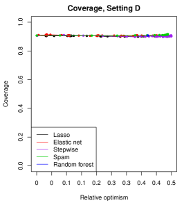
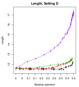
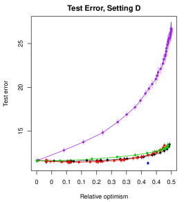
Figure 6: More comparisons of conformal prediction intervals in high-dimensional problems with $n=200$, $d=2000$; here the setup mimics Setting A of Figure 2, but without sparsity: the number of active variables in the linear model for the mean is $s=100$.

Figure 7 displays the results for the same simulation setup as in Figure 3, but without heteroskedasticity in the noise distribution. We can see that the locally-weighted method produces a band with only mildly varying local length, and with essentially constant local coverage. Overall, the average length of the locally-weighted method is not much worse than the usual unweight conformal method.

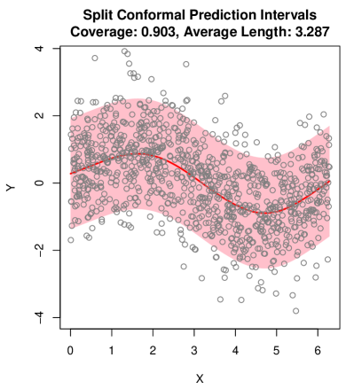
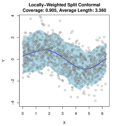
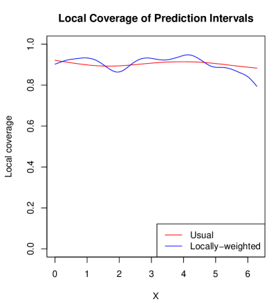
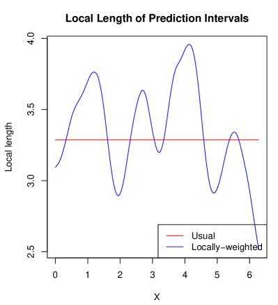
Figure 7: Another example of the usual (unweighted) split conformal and locally-weighted split conformal prediction bands, in the same setup as Figure 3, except without heteroskedasticity.

References

- Belloni et al. (2012) Belloni, A., Chen, D., Chernozhukov, V., & Hansen, C. (2012). Sparse models and methods for optimal instruments with an application to eminent domain. Econometrica, 80(6), 2369–2429.
- Berk et al. (2013) Berk, R., Brown, L., Buja, A., Zhang, K., & Zhao, L. (2013). Valid post-selection inference. Annals of Statistics, 41(2), 802–837.
- Bickel et al. (2009) Bickel, P. J., Ritov, Y., & Tsybakov, A. B. (2009). Simultaneous analysis of lasso and dantzig selector. The Annals of Statistics, (pp. 1705–1732).
- Breiman (2001) Breiman, L. (2001). Random forests. Machine Learning, 45(1), 5–32.
- Buhlmann (2013) Buhlmann, P. (2013). Statistical significance in high-dimensional linear models. Bernoulli, 19(4), 1212–1242.
- Buja et al. (2014) Buja, A., Berk, R., Brown, L., George, E., Pitkin, E., Traskin, M., Zhang, K., & Zhao, L. (2014). Models as approximations: How random predictors and model violations invalidate classical inference in regression. ArXiv: 1404.1578.
- Bunea et al. (2007) Bunea, F., Tsybakov, A., & Wegkamp, M. (2007). Sparsity oracle inequalities for the lasso. Electronic Journal of Statistics, 1, 169–194.
- Burnaev & Vovk (2014) Burnaev, E., & Vovk, V. (2014). Efficiency of conformalized ridge regression. Proceedings of the Annual Conference on Learning Theory, 25, 605–622.
- Butler & Rothman (1980) Butler, R., & Rothman, E. (1980). Predictive intervals based on reuse of the sample. Journal of the American Statistical Association, 75(372), 881–889.
- Efroymson (1960) Efroymson, M. A. (1960). Multiple regression analysis. In Mathematical Methods for Digital Computers, vol. 1, (pp. 191–203). Wiley.
- Fithian et al. (2014) Fithian, W., Sun, D., & Taylor, J. (2014). Optimal inference after model selection. ArXv: 1410.2597.
- Hebiri (2010) Hebiri, M. (2010). Sparse conformal predictors. Statistics and Computing, 20(2), 253–266.
- Javanmard & Montanari (2014) Javanmard, A., & Montanari, A. (2014). Confidence intervals and hypothesis testing for high-dimensional regression. Journal of Machine Learning Research, 15, 2869–2909.
- Lee et al. (2016) Lee, J., Sun, D., Sun, Y., & Taylor, J. (2016). Exact post-selection inference, with application to the lasso. Annals of Statistics, 44(3), 907–927.
- Lei (2014) Lei, J. (2014). Classification with confidence. Biometrika, 101(4), 755–769.
- Lei et al. (2015) Lei, J., Rinaldo, A., & Wasserman, L. (2015). A conformal prediction approach to explore functional data. Annals of Mathematics and Artificial Intelligence, 74(1), 29–43.
- Lei et al. (2013) Lei, J., Robins, J., & Wasserman, L. (2013). Distribution free prediction sets. Journal of the American Statistical Association, 108, 278–287.
- Lei & Wasserman (2014) Lei, J., & Wasserman, L. (2014). Distribution-free prediction bands for non-parametric regression. Journal of the Royal Statistical Society: Series B, 76(1), 71–96.
- Meinshausen & Buhlmann (2010) Meinshausen, N., & Buhlmann, P. (2010). Stability selection. Journal of the Royal Statistical Society: Series B, 72(4), 417–473.
- Papadopoulos et al. (2002) Papadopoulos, H., Proedrou, K., Vovk, V., & Gammerman, A. (2002). Inductive confidence machines for regression. In Machine Learning: ECML 2002, (pp. 345–356). Springer.
- Ravikumar et al. (2009) Ravikumar, P., Lafferty, J., Liu, H., & Wasserman, L. (2009). Sparse additive models. Journal of the Royal Statistical Society: Series B, 71(5), 1009–1030.
- Steinberger & Leeb (2016) Steinberger, L., & Leeb, H. (2016). Leave-one-out prediction intervals in linear regression models with many variables. ArXiv: 1602.05801.
- Thakurta & Smith (2013) Thakurta, A. G., & Smith, A. (2013). Differentially private feature selection via stability arguments, and the robustness of the lasso. In Conference on Learning Theory, (pp. 819–850).
- Tian & Taylor (2015a) Tian, X., & Taylor, J. (2015a). Asymptotics of selective inference. ArXiv: 1501.03588.
- Tian & Taylor (2015b) Tian, X., & Taylor, J. (2015b). Selective inference with a randomized response. ArXiv: 1507.06739.
- Tibshirani (1996) Tibshirani, R. (1996). Regression shrinkage and selection via the lasso. Journal of the Royal Statistical Society: Series B, 58(1), 267–288.
- Tibshirani et al. (2016) Tibshirani, R. J., Taylor, J., Lockhart, R., , & Tibshirani, R. (2016). Exact post-selection inference for sequential regression procedures. Journal of the American Statistical Association, 111(514), 600–620.
- van de Geer et al. (2014) van de Geer, S., Buhlmann, P., Ritov, Y., & Dezeure, R. (2014). On asymptotically optimal confidence regions and tests for high-dimensional models. Annals of Statistics, 42(3), 1166–1201.
- Vovk (2013) Vovk, V. (2013). Conditional validity of inductive conformal predictors. Machine Learning, 92, 349–376.
- Vovk et al. (2005) Vovk, V., Gammerman, A., & Shafer, G. (2005). Algorithmic Learning in a Random World. Springer.
- Vovk et al. (2009) Vovk, V., Nouretdinov, I., & Gammerman, A. (2009). On-line predictive linear regression. The Annals of Statistics, 37(3), 1566–1590.
- Wasserman (2014) Wasserman, L. (2014). Discussion: A significance test for the lasso. Annals of Statistics, 42(2), 501–508.
- Zhang & Zhang (2014) Zhang, C.-H., & Zhang, S. (2014). Confidence intervals for low dimensional parameters in high dimensional linear models. Journal of the Royal Statistical Society: Series B, 76(1), 217–242.
- Zou & Hastie (2005) Zou, H., & Hastie, T. (2005). Regularization and variable selection via the elastic net. Journal of the Royal Statistical Society: Series B, 67(2), 301–320.