1-bit Matrix Completion: PAC-Bayesian Analysis of a Variational Approximation

Abstract

Due to challenging applications such as collaborative filtering, the matrix completion problem has been widely studied in the past few years. Different approaches rely on different structure assumptions on the matrix in hand. Here, we focus on the completion of a (possibly) low-rank matrix with binary entries, the so-called 1-bit matrix completion problem. Our approach relies on tools from machine learning theory: empirical risk minimization and its convex relaxations. We propose an algorithm to compute a variational approximation of the pseudo-posterior. Thanks to the convex relaxation, the corresponding minimization problem is bi-convex, and thus the method behaves well in practice. We also study the performance of this variational approximation through PAC-Bayesian learning bounds. On the contrary to previous works that focused on upper bounds on the estimation error of $M$ with various matrix norms, we are able to derive from this analysis a PAC bound on the prediction error of our algorithm.

We focus essentially on convex relaxation through the hinge loss, for which we present the complete analysis, a complete simulation study and a test on the MovieLens data set. However, we also discuss a variational approximation to deal with the logistic loss.

1 Introduction

Motivated by modern applications like recommendation systems and collaborative filtering, video analysis or quantum statistics, the matrix completion problem has been widely studied in the recent years. Recovering a matrix which is, without any additional information, a purely impossible task. Actually, in general, it is obviously impossible. However, under some assumption on the structure of the matrix to be recovered, it might become feasible, as shown by [8] and [7] where the assumption is that the matrix has a small rank. This assumption is indeed very natural in many applications. For example, in recommendation systems, it is equivalent to the existence of a small number of hidden features that explain the preferences of users. While [8] and [7] focused on matrix completion without noise, many authors extended these techniques to the case of noisy observations, see [6] and  [11] among others. The main idea in [6] is to minimize the least squares criterion, penalized by the rank. This penalization is then relaxed by the nuclear norm, which is the sum of the singular values of the matrix at hand. An efficient algorithm is described in [24].

All the aforementioned papers focused on real-valued matrices. However, in many applications, the matrix entries are binary, that is in the set $\{0,1\}$. For example, in collaborative filtering, the $(i,j)-th$ entry being $1$ means that user $i$ likes object $j$ while this entry being $0$ means that he/she dislikes it. The problem of recovering a binary matrix from partial observations is usually referred as 1-bit matrix completion. To deal with binary observations requires specific estimation methods. Most works on this problem usually assume a generalized linear model (GLM): the observations $Y_{ij}$ for $1\leq i\leq m_{1}$, $1\leq j\leq m_{2}$, are Bernoulli distributed with parameter $f(M_{ij})$, where $f$ is a link function which maps from $\mathbb{R}$ to $[0,1]$, for example the logistic function $f(x)=\exp(x)/[1+\exp(x)]$, and $M$ is a $m_{1}\times m_{2}$ real matrix, see [5, 13, 16]. In these works, the goal is to recover the matrix $M$ and a convergence rate is then derived. For example, [16] provides an estimate $\widehat{M}$ for which, under suitable assumptions and when the data are generated according to the true model with $M=M_{0}$,

$$\frac{1}{m_{1}m_{2}}\|\widehat{M}-M_{0}\|_{F}^{2}\leq C\max\left(\frac{1}{\sqrt{n}},\frac{(m_{1}\vee m_{2}){\rm rank(M_{0})}}{n}\right)$$

for some constant $C$ that depends on the assumptions, and where $\|.\|_{F}$ stands for the Frobenius norm (we refer the reader to Corollary 2 page 1955 in [16] for the exact statement). While this result ensures the consistency of $\widehat{M}$ when $M_{0}$ is low-rank, it does not provide any guarantee on the probability of a prediction error. Moreover, such a prediction there would necessarily assume that the model is correct, that is, that the link function $f$ is well specified, which is an unrealistic assumption.

Here, we adopt a machine learning point of view: in machine learning, dealing with binary output is called a classification problem, for which methods are known that do not assume any model on the observations. That is, instead of focusing on a parametric model for $Y_{i,j}$, we will only define a set of prediction matrices $M$ and seek for the one that leads to the best prediction error. Using the 0-1 loss function, we could actually directly use Vapnik-Chervonenkis theory [29] to propose a classifier $\hat{M}$ risk would be controled by a PAC inequality. However, it is known that this approach usually is computationally intractable. A popular approach is to replace the 0-1 loss by a convex surrogate [30], namely, the hinge loss. Our approach is as follows: we propose a pseudo-Bayesian approach, where we define a pseudo-posterior distribution on a set of matrices $M$. This pseudo-posterior distribution does not have a very simple form, however, thanks to a variational approximation, we manage to approximate it by a tractable distribution. Thanks to the PAC-Bayesian theory [22, 14, 27, 9, 10, 26, 12], we are able to provide a PAC bound on the prediction risk of this variational approximation. We then show that, thanks to the convex relaxation of the 0-1 loss, the computation of this variational approximation is actually a bi-convex minimization problem. As a consequence, algorithms that are efficient in practice are available.

The rest of the paper is as follows. In Section 2 we provide the notations used in the paper, the definition of the pseudo-posterior and of its variational approximation. In Section 3 we give the PAC analysis of the variational approximation. This allows an empirical and a theoretical upper bound on the prevision risk of our method. Section 4 provides details on the implementation of our method. Note that in the aforementioned sections, the convex surrogate of the 0-1 loss used is the hinge loss. An extension to the logistic loss is briefly discussed in Section 5 and the derived algorithm to compute the variational approximation. Finally, Section 6 is devoted to an empirical study and Section 6.2 to an application to the MovieLens data set. The proof of the theorems of Section 3 are provided in Section 8.

2 Notations

For any integer $m$ we define $[m]=\{1,\dots,m\}$. We define, for any integers $m$ and $k$ and any matrix $M\in\mathbb{R}^{m\times k}$, $\|M\|_{\textrm{max}}=\max_{(i,j)\in[m]\times[k]}M_{ij}$. For a pair of matrices $(M,N)$, we write $\ell(M,N)=\|M\|_{\textrm{max}}\vee\|N\|_{\textrm{max}}$. Finally, when an $m\times k$ matrix $M$ has rank ${\rm rank}(M)=\ell$ then it can be written as $M=UV^{T}$ where $U$ is $m\times\ell$ and $V$ is $k\times\ell$. This decomposition is obviously not unique; we put $\ell(M)=\inf_{(U,V)}\ell(U,V)$ where the infimum is taken over all such possible pairs $(U,V)$.

2.1 1-bit matrix completion as a classification problem

We formally describe the 1-bit matrix completion problem as a classification problem: we observe $(X_{k},Y_{k})_{k\in[n]}$ that are $n$ i.i.d pairs from a distribution $\mathbf{P}$. The $X_{k}$’s take values in $\mathcal{X}=[m_{1}]\times[m_{2}]$ and the $Y_{k}$’s take values in $\mathcal{Y}=\{-1,+1\}$. Hence, the $k$-th observation of an entry of the matrix is $Y_{k}$ and the corresponding position in the matrix is provided by $X_{k}=(i_{k},j_{k})$. In this setting, a predictor is a function $[m_{1}]\times[m_{2}]\rightarrow\mathbb{R}$ and thus can be represented by a matrix $M$. It would be natural to use $M$ in the following way: when $(X,Y)\sim\mathbf{P}$, $M$ predicts $Y$ by ${\rm sign}(M_{X})$. The ability of this predictor to predict a new entry of the matrix is then assessed by the risk

$$R(M)=\mathbb{E}_{\mathbf{P}}\left[\mathbbm{1}(YM_{X}<0)\right],$$

and its empirical counterpart is:

$$r_{n}(M)=\frac{1}{n}\sum_{k=1}^{n}\mathbbm{1}(Y_{k}M_{X_{k}}<0)=\frac{1}{n}\sum_{k=1}^{n}\mathbbm{1}(Y_{k}M_{i_{k},j_{k}}<0).$$

It is then possible to use the standard approach in classification theory [29]. For example, the best possible classifier is the Bayes classifier

$$\eta(x)=\mathbb{E}(Y|X=x)\quad\textrm{or equivalently}\quad\eta(i,j)=\mathbb{E}[Y|X=(i,j)],$$

and equivalently we have a corresponding optimal matrix

$$M^{B}_{ij}=\textrm{sign}[\eta(i,j)]=\textrm{sign}\Bigl{\{}\mathbb{E}[Y|X=(i,j)]\Bigr{\}}.$$

We define $\overline{R}=\inf_{M}R(M)=R(M^{B})$, and $\overline{r_{n}}=r_{n}(M^{B})$. Note that, clearly, if two matrices $M^{1}$ and $M^{2}$ are such as, for every $(i,j)$, $\textrm{sign}(M^{1}_{ij})=\textrm{sign}(M^{2}_{ij})$ then $R(M^{1})=R(M^{2})$, and obviously,

$$\forall M,\forall(i,j)\in[m_{1}]\times[m_{2}],\quad\textrm{sign}(M_{ij})=M^{B}_{ij}\quad\Rightarrow\quad r_{n}(M)=\overline{r_{n}}.$$

While the risk $R(M)$ has a clear interpretation, it is well known that to work with its empirical counterpart $r_{n}(M)$ usually leads to intractable problems, as it is non-smooth and non-convex. Hence, it is quite standard to replace the empirical risk by a convex surrogate [30]. In this paper, we will mainly deal with the hinge loss, which leads to the following so-called hinge risk and hinge empirical risk:

$$R^{h}(M) =\mathbb{E}_{\mathbf{P}}\left[(1-YM_{X})_{+}\right],$$

$$r_{n}^{h}(M) =\frac{1}{n}\sum_{k=1}^{n}(1-Y_{k}M_{X_{k}})_{+}.$$

Note that the hinge loss was also used by [28] in the 1-bit matrix completion problem, with a different approach leading to different algorithms. Moreover, here, we provide an analysis of the rate of convergence of our method, that is not provided in [28].

In opposite to other matrix completion works, the marginal distribution of $X$ is not an issue and we do not consider an uniform sampling scheme. Another slight difference is that the observations are iid and a same index may be observed several times. Following standard notations in matrix completion, we can define $\Omega$ as the set of indices of observed entries: $\Omega=\{X_{1},\dots,X_{n}\}$. We will use in the following the sub-sample of $\left\{1,\dots,n\right\}$ for a specified line $i$: $\Omega_{i,\cdot}=\left\{l\in[n]:(i,j_{l})\in\Omega\right\}$ and the counterpart for a specified column $j$: $\Omega_{\cdot,j}=\left\{l\in[n]:(i_{l},j)\in\Omega\right\}$.

2.2 Pseudo-Bayesian estimation

The Bayesian framework has been used several times for matrix completion [20, 25, 19]. A common idea in all these papers is to factorize the matrix into two parts in order to define a prior on low-rank matrices. Every matrix whose rank is $r$ can be factorized:

$$M=LR^{\top},L\in\mathbb{R}^{m_{1}\times r},\quad R\in\mathbb{R}^{m_{2}\times r}.$$

As mentioned in the introduction, this is motivated by the fact that we expect that the Bayes matrix $M^{B}$ is low-rank, or at least well approximated by a low-rank matrix. However, in practice, we do not know what would be the rank of this matrix. So, we actually write $M=LR^{\top}$ with $L\in\mathbb{R}^{m_{1}\times K}$, $R\in\mathbb{R}^{m_{2}\times K}$ for some large enough $K$, and then, seek for adaptation with respect to a possible rank $r\in[K]$ by shrinking some columns of $L$ and $R$ to $0$. Specifically, we define the prior as the following hierarchical model:

$$\forall k\in[K],\quad\gamma_{k} \stackrel{{\scriptstyle iid}}{{\sim}}\pi^{\gamma},$$

$$\forall(i,j)\in[m_{1}]\times[m_{2}],\quad L_{i,\cdot},R_{j,\cdot}|\gamma \stackrel{{\scriptstyle iid}}{{\sim}}\mathcal{N}(0,\textrm{diag}(\gamma)),$$

$$\text{ and }M =LR^{\top},$$

where the prior distribution on the variances $\pi^{\gamma}$ is yet to be specified. Usually $\pi^{\gamma}$ is an inverse-Gamma distribution because it is conjugate in this model. This kind of hierarchical prior distribution is also very similar to the Bayesian Lasso developed in [23] and especially of the form of the Bayesian Group Lasso developed in [17] in which the variance term is Gamma distributed. We will show that the Gamma distribution is a possible alternative in matrix completion, both for theoretical results and practical considerations. Thus all the results in this paper are stated under the assumption that $\pi^{\gamma}$ is either the Gamma or the inverse-Gamma distribution: $\pi^{\gamma}=\Gamma(\alpha,\beta)$, or $\pi^{\gamma}=\Gamma^{-1}(\alpha,\beta)$.

Let $\theta$ denote the parameter $\theta=(L,R,\gamma)$. As in PAC-Bayes theory [10], we define the pseudo-posterior as follows:

$$\widehat{\rho}_{\lambda}(d\theta)=\frac{\exp[-\lambda r_{n}^{h}(LR^{\top})]}{\int\exp[-\lambda r_{n}^{h}]d\pi}\pi(d\theta)$$

where $\lambda>0$ is a parameter to be fixed by the statistician. The calibration of $\lambda$ is discussed below. This distribution is close to a classic posterior distribution but the log-likelihood has been replaced by the logarithm of the pseudo-likelihood $r_{n}^{h}(LR^{\top})$ based on the hinge empirical risk.

2.3 Variational Bayes approximations

Unfortunately, the pseudo-posterior is intractable and MCMC methods are too expensive because of the dimension of the parameter. A possible way in order to get an estimate is to seek an approximation of this distribution. A specific technique, known as Variational Bayes (VB) approximation, allows to replace MCMC methods by efficient optimization algorithms [2]. First, we fix a subset $\mathcal{F}$ of the set of all distributions on the parameter space. The class $\mathcal{F}$ should be large enough, in order to contain a good enough approximation of $\widehat{\rho}_{\lambda}$, but not too large in order to lead to tractable optimization problems. We usually define the VB approximation as $\arg\min_{\rho\in\mathcal{F}}\mathcal{K}(\rho,\widehat{\rho})$. However, when $\mathcal{K}(\rho,\widehat{\rho})$ is not available in close form, it is usual to replace it by an upper bound. We define here the class $\mathcal{F}$ as follows:

$$\mathcal{F}=\Biggl{\{}\rho(d(L,R,\gamma)) =\prod_{k=1}^{K}\left[\prod_{i=1}^{m_{1}}\varphi(L_{i,k};L_{i,k}^{0},v_{i,k}^{L})\prod_{j=1}^{m_{2}}\varphi(R_{j,k};R_{j,k}^{0},v_{j,k}^{R})\rho^{\gamma_{k}}(d\gamma_{k})\right],$$

$$L^{0}\in\mathbb{R}^{m_{1}\times K},R^{0}\in\mathbb{R}^{m_{2}\times K},v^{L}\in\mathbb{R}_{+}^{m_{1}\times K},v^{R}\in\mathbb{R}_{+}^{m_{2}\times K}\Biggr{\}},$$

where $\varphi(.,\mu,v)$ is the density of the Gaussian distribution with parameters $(\mu,v)$ and $\rho^{\gamma_{k}}$ ranges over all possible probability distributions for $\gamma^{k}\in\mathbb{R}^{+}$. Note that VB approximations are referred as parametric when $\mathcal{F}$ is finite dimensional and as mean-field otherwise, then we actually use a mixed approach. Informally, all the coordinates are independent and the variational distribution of the entries of $L$ and $R$ is specified. The free variational parameters to be optimized are the means and the variances, which can be both seen in a matrix form. We will show below that the optimization with respect to $\rho^{\gamma_{k}}$ is available in close form. Also, note that any probability distribution $\rho\in\mathcal{F}$ is uniquely determined by $L^{0}$, $R^{0}$, $v^{L}$, $v^{R}$ and $\rho^{\gamma_{1}},\dots,\rho^{\gamma_{k}}$. We could actually use the notation $\rho=\rho_{L^{0},R^{0},v^{L},v^{R},\rho^{\gamma_{1}},\dots,\rho^{\gamma_{k}}}$, but it would be too cumbersome, so we will avoid it as much as possible. Conversely, once $\rho$ is given in $\mathcal{F}$, we can define $L^{0}=\mathbb{E}_{\rho}[L]$, $R^{0}=\mathbb{E}_{\rho}[R]$ and so on.

The Kullback divergence here decomposes as

$$\mathcal{K}(\rho,\widehat{\rho}_{\lambda})=\lambda\int r_{n}^{h}d\rho+\mathcal{K}(\rho,\pi)+\log\int\exp[-\lambda r_{n}^{h}]d\pi$$ (1)

for which we do not have a close form, so we rather minimize an upper bound. We will see in next sections that this estimate has actually very good properties.

Definition 1.

Let $\rho=\rho_{L^{0},R^{0},v^{L},v^{R},\rho^{\gamma_{1}},\dots,\rho^{\gamma_{k}}}\in\mathcal{F}$ and

$$\mathcal{R}(\rho,\lambda) =\frac{1}{n}\sum_{\ell=1}^{n}\sum_{k=1}^{K}\left[\sqrt{v^{L}_{i_{\ell},k}\frac{2}{\pi}}\sqrt{v^{R}_{j_{\ell},k}\frac{2}{\pi}}+|R_{j_{\ell},k}^{0}|\sqrt{v^{L}_{i_{\ell},k}\frac{2}{\pi}}+|L_{i_{\ell},k}^{0}|\sqrt{v^{R}_{j_{\ell},k}\frac{2}{\pi}}\right]$$

$$+\frac{1}{\lambda}\left(\frac{1}{2}\sum_{k=1}^{K}\mathbb{E}_{\rho}\left[\frac{1}{\gamma_{k}}\right]\left(\sum_{i=1}^{m_{1}}(v^{L}_{ik}+L^{02}_{ik})+\sum_{j=1}^{m_{2}}(v^{R}_{jk}+R^{02}_{jk})\right)-\frac{1}{2}\sum_{k=1}^{K}\left(\sum_{i=1}^{m_{1}}\log v^{L}_{ik}+\sum_{j=1}^{m_{2}}\log v^{R}_{jk}\right)\right.$$

$$\left.+\sum_{k=1}^{K}\left[\mathcal{K}(\rho^{\gamma_{k}},\pi^{\gamma})+\frac{m_{1}+m_{2}}{2}\left(\mathbb{E}_{\rho}\left[\log\gamma_{k}\right]-1\right)\right]\right).$$

Proposition 1.

For any $\rho$ in $\mathcal{F}$,

$$\int r_{n}^{h}d\rho+\frac{1}{\lambda}\mathcal{K}(\rho,\pi)\leq r_{n}^{h}\left(\mathbb{E}_{\rho}[L]\mathbb{E}_{\rho}[R]^{\top}\right)+\mathcal{R}(\rho,\lambda).$$ (2)

We remind the reader that all the proofs are in Section 8. The quantity $r_{n}^{h}\left(\mathbb{E}_{\rho}[L]\mathbb{E}_{\rho}[R]^{\top}\right)+\mathcal{R}(\rho,\lambda)$ will be referred to as the Approximate Variational Bound (AVB) in the following. We are now able to define our estimate.

Definition 2.

We put

$$AVB(\rho) =r_{n}^{h}\left(\mathbb{E}_{\rho}[L]\mathbb{E}_{\rho}[R]^{\top}\right)+\mathcal{R}(\rho,\lambda),$$

$$\widetilde{\rho}_{\lambda} =\arg\min_{\rho\in\mathcal{F}}AVB(\rho).$$ (3)

Also, for simplicity, given $L^{0},R^{0},v^{L},v^{R},\rho^{\gamma_{1}},\dots,\rho^{\gamma_{k}}$ we will use the notation

$$AVB(L^{0},R^{0},v^{L},v^{R},\rho^{\gamma_{1}},\dots,\rho^{\gamma_{k}})=AVB(\rho_{L^{0},R^{0},v^{L},v^{R},\rho^{\gamma_{1}},\dots,\rho^{\gamma_{k}}}).$$

3 PAC analysis of the variational approximation

Paper [1] proposes a general framework for analyzing the prediction properties of VB approximations of pseudo-posteriors based on PAC-Bayesian bounds. In this section, we apply this method to derive a control of the out-of-sample prevision risk $R$ for our approximation $\widetilde{\rho}_{\lambda}$.

3.1 Empirical Bound

The first result is a so-called empirical bound: it provides an upper bound on the prevision risk of the pseudo-posterior $\widetilde{\rho}_{\lambda}$ that depends only on the data and on quantities defined by the statistician.

Theorem 1.

For any $\epsilon\in(0,1)$, with probability at least $1-\epsilon$ on the drawing of the sample,

$$\int Rd\widetilde{\rho}_{\lambda}\leq\inf_{\rho\in\mathcal{F}}\left[r_{n}^{h}\left(\mathbb{E}_{\rho}[L]\mathbb{E}_{\rho}[R]^{\top}\right)+\mathcal{R}(\rho,\lambda)\right]+\frac{\lambda}{2n}+\frac{\log\frac{1}{\epsilon}}{\lambda}$$

We can actually deduce from this result a more explicit bound.

Corollary 1.

Assume that $\lambda\leq n$. For any $\epsilon\in(0,1)$,with probability at least $1-\epsilon$:

$$\int Rd\widetilde{\rho}_{\lambda}\leq\inf_{M}\left[r_{n}^{h}\left(M\right)+\mathcal{C}_{\pi^{\gamma}}\frac{{\rm rank}(M)(m_{1}+m_{2})[\log n+\ell^{2}(M)]}{\lambda}\right]+\frac{\lambda}{2n}+\frac{\log\frac{1}{\epsilon}}{\lambda}$$

where the constant $\mathcal{C}_{\pi^{\gamma}}$ is explicitely known, and depends only on the prior $\pi^{\gamma}$ (Gamma, or Inverse-Gamma) and of the hyperparameters.

An exact value for $\mathcal{C}_{\pi^{\gamma}}$ can be deduced from the proof. It is thus clear that the algorithm performs a trade-off between the fit to the data, through the term $r_{n}^{h}(LM)$, and the rank of $M$.

3.2 Theoretical Bound

For this bound, it is common in classification to make an additional assumption on $\mathbf{P}$ which leads to an easier task and therefore to better rates of convergence. We propose a definition adapted from [21].

Definition 3.

Mammen and Tsybakov’s margin assumption is satisfied when there is a constant $C$ such that:

$$\mathbb{E}\left[\left(\mathbbm{1}_{YM_{X}\leq 0}-\mathbbm{1}_{YM^{B}_{X}\leq 0}\right)^{2}\right]\leq C[R(M)-\overline{R}].$$

It is known that it there is a constant $C^{\prime}>0$ such that $\mathbb{P}(0<|\eta(X)|\leq t)\leq C^{\prime}t$ then the margin assumption is satisfied with some $C$ that depends on $C^{\prime}$. For example, in the noiseless case where $Y=M^{B}_{X}$ almost surely, then

$$\mathbb{E}\left[\left(\mathbbm{1}_{YM_{X}\leq 0}-\mathbbm{1}_{YM^{B}_{X}\leq 0}\right)^{2}\right]=\mathbb{E}\left[\mathbbm{1}_{YM_{X}\leq 0}^{2}\right]=\mathbb{E}\left[\mathbbm{1}_{YM_{X}\leq 0}\right]=R(M)=R(M)-\overline{R},$$

so the margin assumption is satisfied with $C=1$.

Theorem 2.

Assume that the Mammen and Tsybakov’s assumption is satisfied for a given constant $C>0$. Then, for any $\epsilon\in(0,1)$ and for $\lambda=sn/C$, $s\in(0,1)$, with probability at least $1-2\epsilon$,

$$\int Rd\widetilde{\rho}_{\lambda}\leq 2(1+3s)\overline{R}+\mathcal{C}_{C,c,\pi^{\gamma}}\left(\frac{{\rm rank}(M^{B})(m_{1}+m_{2})[\log n+\ell^{2}(M^{B})]+\log\left(\frac{1}{\epsilon}\right)}{n}\right)$$

where $\mathcal{C}_{C,s,\pi^{\gamma}}$ is known and depends only on the constants $s,C$ and the choice of the prior on $\gamma$.

Note the adaptive nature of this result, in the sense that the estimator does not depend on ${\rm rank}(M^{B})$.

Corollary 2.

In the noiseless case $Y={\rm sign}(M^{B}_{X})$ a.s., for any $\epsilon>0$ and for $\lambda=2n$, with probability at least $1-2\epsilon$,

$$\int Rd\widetilde{\rho}_{\lambda}\leq\mathcal{C}^{\prime}_{\pi^{\gamma}}\left[\frac{{\rm rank}(M^{B})(m_{1}+m_{2})[\log n+\ell^{2}(M^{B})]+\log\frac{1}{\epsilon}}{n}\right]$$ (4)

where $\mathcal{C}^{\prime}_{\pi^{\gamma}}=\mathcal{C}_{1,\frac{1}{4},1,\pi^{\gamma}}$.

Remark 1.

Note that an empirical inequality roughly similar to Corollary 1 appears in [28]. However, in this paper, no oracle inequality similar to Corollary 2 is derived - and, due to a slight modification in their definition of the empirical hinge risk, we believe that it would not be easy to derive such a bound from their techniques.

4 Algorithm

4.1 General Algorithm

Note that the minimization problem (3) that defines our VB approximation is not an easy one:

$$\min_{L^{0},R^{0},v^{L},v^{R},\rho^{\gamma_{1}},\dots,\rho^{\gamma_{k}}}AVB(L^{0},R^{0},v^{L},v^{R},\rho^{\gamma_{1}},\dots,\rho^{\gamma_{k}}).$$

When $v^{L}$, $v^{R}$ and all the $\rho^{\gamma_{k}}$’s are fixed, this is actually the canonical example of so-called biconvex problems: it is convex with respect to $L^{0}$, and with respect to $R^{0}$, but not with respect to the pair $(L^{0},R^{0})$. Such problems are notoriously difficult. In this case, alternating blockwise optimization seems to be an acceptable strategy. While there is no guarantee that the algorithm will not get stuck in a local minimum (or even in a singular point that is actually not a minimum), it seems to give good results in practice, and no efficient alternative is available. See the discussion Subsection 9.2 page 76 in [4] for more details on this problem. We update iteratively $L^{0},R^{0},v^{L},v^{R},\rho^{\gamma_{1}},\dots,\rho^{\gamma_{k}}$: for $L^{0}$ and $R^{0}$ we use a gradient step, while for $v^{L},v^{R},\rho^{\gamma_{1}},\dots,\rho^{\gamma_{k}}$ an explicit minimization is available. The details for the mean-field optimization (that is, w.r.t. $\rho^{\gamma_{1}},\dots,\rho^{\gamma_{k}}$) are given in Subsection 4.2. See Algorithm 1 for the general version of the algorithm.

Algorithm 1 Variational Approximation with Hinge Loss

0:  $\epsilon,(\eta_{t})_{t\in\mathbb{N}},L^{0}_{0},R^{0}_{0},v^{L}_{0},v^{R}_{0},\rho^{\gamma}_{0}$

  $t\leftarrow 0$

  while $\|L_{t}^{0}R_{t}^{0\top}-L_{t-1}^{0}R_{t-1}^{0\top}\|_{F}^{2}\leq\epsilon$ do

     $t\leftarrow t+1$

     $L^{0}_{t}\leftarrow L^{0}_{t-1}-\eta_{t}\frac{\partial AVB}{\partial L^{0}}(L^{0}_{t-1},R^{0}_{t-1},v^{L}_{t-1},v^{R}_{t-1},\rho^{\gamma_{1}}_{t-1},\dots,\rho^{\gamma_{K}}_{t-1})$

     $R^{0}_{t}\leftarrow R^{0}_{t-1}-\eta_{t}\frac{\partial AVB}{\partial R^{0}}(L^{0}_{t},R^{0}_{t-1},v^{L}_{t-1},v^{R}_{t-1},\rho^{\gamma_{1}}_{t-1},\dots,\rho^{\gamma_{K}}_{t-1})$

     $v^{L}_{t}\leftarrow\textrm{arg}\min_{v^{L}}AVB(L^{0}_{t},R^{0}_{t},v^{L},v^{R}_{t-1},\rho^{\gamma_{1}}_{t-1},\dots,\rho^{\gamma_{K}}_{t-1})$

     $v^{R}_{t}\leftarrow\textrm{arg}\min_{v^{R}}AVB(L^{0}_{t},R^{0}_{t},v^{L}_{t},v^{R},\rho^{\gamma_{1}}_{t-1},\dots,\rho^{\gamma_{K}}_{t-1})$

     $(\rho^{\gamma_{1}}_{t},\dots,\rho^{\gamma_{K}}_{t})\leftarrow\textrm{arg}\min_{\rho^{\gamma_{1}},\dots,\rho^{\gamma_{K}}}AVB(L^{0}_{t},R^{0}_{t},v^{L}_{t},v^{R},\rho^{\gamma_{1}},\dots,\rho^{\gamma_{K}})$

  end while

4.2 Mean Field Optimization

Note that the pseudo-likelihood does not involve the parameters $(\gamma_{1},\dots,\gamma_{K})$ so the variational distribution can be optimized in the same way as the model in [19] where the noise is Gaussian. The general update formula is ($\rho^{-\gamma_{k}}$ stands for the whole distribution $\rho$ except the part involving $\gamma_{k}$):

$$\rho^{\gamma_{k}}(\gamma_{k}) \propto\exp\mathbb{E}_{\rho^{-\gamma_{k}}}\left(\log\pi(L,R,\gamma)\right)$$

$$\propto\exp\mathbb{E}_{\rho^{-\gamma_{k}}}\left(\log[\pi(L|\gamma)\pi(R|\gamma)\pi^{\gamma}(\gamma)]\right)$$

$$\propto\exp\left\{\sum_{i=1}^{m_{1}}\mathbb{E}_{\rho^{L}}\left[\log\pi(L_{i,k}|\gamma_{k})\right]+\sum_{j=1}^{m_{2}}\mathbb{E}_{\rho^{R}}\left[\log\pi(R_{j,k}|\gamma_{k})\right]+\log\pi^{\gamma}\left(\gamma_{k}\right)\right\}$$

$$\propto\exp\left\{-\frac{m_{1}+m_{2}}{2}\log\gamma_{k}-\frac{1}{\gamma_{k}}\mathbb{E}_{\rho}\left[\frac{\sum_{i=1}^{m_{1}}L_{i,k}^{2}+\sum_{j=1}^{m_{2}}R_{j,k}^{2}}{2}\right]+\log\pi^{\gamma}\left(\gamma_{k}\right)\right\}.$$

The solution then depends on $\pi^{\gamma}$. In what follows we derive explicit formulas for $\rho^{\gamma_{k}}$ according to the choice of $\pi^{\gamma}$: remember that $\pi^{\gamma}$ could be either a Gamma distribution, or an Inverse-Gamma distribution.

4.2.1 Inverse-Gamma Prior

The conjugate prior for this part of the model is the inverse-Gamma distribution. The prior of $\gamma_{k}$ is $\pi^{\gamma}=\Gamma^{-1}(\alpha,\beta)$ and its density is:

$$\pi^{\gamma}(\gamma_{k};\alpha,\beta)=\frac{\beta^{\alpha}}{\Gamma(\alpha)}\gamma_{k}^{-\alpha-1}\exp\left(-\frac{\beta}{\gamma_{k}}\right)\mathbbm{1}_{\mathbb{R}^{+}}(\gamma_{k}).$$

The moments we need to develop the algorithm and to compute the empirical bound are:

$$\mathbb{E}_{\pi^{\gamma}}(\log\gamma_{k})=\log\beta-\psi(\alpha)\text{, and }\mathbb{E}_{\pi^{\gamma}}(1/\gamma_{k})=\frac{\alpha}{\beta},$$

where $\psi$ is the digamma function. Therefore, we get:

$$\rho^{\gamma_{k}}(\gamma_{k}) \propto\exp\left\{-\left(\frac{m_{1}+m_{2}}{2}+\alpha+1\right)\log\gamma^{k}-\frac{1}{\gamma_{k}}\left(\mathbb{E}_{\rho}\left[\frac{\sum_{i=1}^{m_{1}}L_{i,k}^{2}+\sum_{j=1}^{m_{2}}R_{j,k}^{2}}{2}\right]+\beta\right)\right\},$$

so we can conclude that:

$$\rho^{\gamma_{k}}=\Gamma^{-1}\left(\frac{m_{1}+m_{2}}{2}+\alpha,\mathbb{E}_{\rho}\left[\frac{\sum_{i=1}^{m_{1}}L_{i,k}^{2}+\sum_{j=1}^{m_{2}}R_{j,k}^{2}}{2}\right]+\beta\right).$$ (5)

4.2.2 Gamma Prior

Even though it seems that this fact was not used in prior works on Bayesian matrix estimation, it is also possible to derive explicit formulas when the prior $\pi^{\gamma}$ on $\gamma_{k}$’s is a $\Gamma(\alpha,\beta)$ distribution. In this case, $\rho^{\gamma_{k}}$ is given by

$$\rho^{\gamma_{k}}(\gamma_{k}) \propto\exp\left\{\left(\alpha-\frac{m_{1}+m_{2}}{2}-1\right)\log\gamma_{k}-\beta\gamma_{k}-\frac{1}{\gamma_{k}}\mathbb{E}_{\rho}\left[\frac{\sum_{i=1}^{m_{1}}L_{i,k}^{2}+\sum_{j=1}^{m_{2}}R_{j,k}^{2}}{2}\right]\right\}.$$

We remind the reader that the Generalized Inverse Gaussian distribution is a three-parameter family of distributions over $\mathbb{R}^{+*}$, written $GIG(a,b,\eta)$. Its density is given by:

$$f(x;a,b,\eta) =\frac{(a/b)^{\eta/2}}{2K_{\eta}(\sqrt{ab})}x^{\eta-1}\exp\left(-\frac{1}{2}(ax+bx^{-1})\right),$$

where $K_{\lambda}$ is the modified Bessel function of second kind.

The variational distribution $\rho^{\gamma_{k}}$ is in consequence $GIG(a_{k},b_{k},\eta_{k})$ with:

$$a_{k} =2\beta,\quad b_{k}=\mathbb{E}_{\rho}\left[\frac{\sum_{i=1}^{m_{1}}L_{i,k}^{2}+\sum_{j=1}^{m_{2}}R_{j,k}^{2}}{2}\right],\quad\eta_{k}=\alpha-\frac{m_{1}+m_{2}}{2}.$$

The moment we need in order to compute the variational distribution of $L,R$ is:

$$\mathbb{E}_{\rho^{\gamma_{k}}}\left(\frac{1}{\gamma_{k}}\right)=\frac{K_{\eta_{k}-1}(\sqrt{a_{k}b_{k}})}{K_{\eta_{k}}(\sqrt{a_{k}b_{k}})}\sqrt{\frac{a_{k}}{b_{k}}}.$$

5 Logistic Model

As mentioned in [30], the hinge loss is not the only possible convex relaxation of the 0-1 loss. The logistic loss ${\rm logit}(u)=\log[1+\exp(-u)]$ can also be used (even though it might lead to a loss in the rate of convergence). This leads to the risks:

$$R^{\ell}(M) =\mathbb{E}_{\mathbf{P}}\left[{\rm logit}(YM_{X})\right],$$

$$r_{n}^{\ell}(M) =\frac{1}{n}\sum_{k=1}^{n}{\rm logit}(Y_{k}M_{X_{k}}).$$

Note that then the pseudo-likelihood $\exp(-\lambda r_{n}^{\ell}(M))$ becomes exactly equal to the likelihood if $\lambda=n$ and we assume a logistic model, that is $Y_{k}=2y_{k}-1$, $y_{k}|X_{k}\in\mathcal{B}e(\sigma(M_{X_{k}}))$ where $\sigma$ is the link function $\sigma(x)=\frac{\exp(x)}{1+\exp(x)}$. For the sake of coherence with previous sections, we still use the machine learning notations and the likelihood is written $\Lambda(L,R)=\prod_{l=1}^{n}\sigma(Y_{l}(LR^{\top})_{X_{l}})$. The prior distribution is exactly the same and the object of interest is the posterior distribution:

$$\widehat{\rho_{l}}(d\theta)=\frac{\Lambda(L,R)\pi(d\theta)}{\int\Lambda(L,R)\pi(d\theta)}.$$

In order to deal with large matrices, it is still interesting to develop a variational Bayes algorithm. However it is not as simple as in the quadratic loss model, see [19] in which the authors develop a mean field approximation, because the logistic likelihood leads to intractable update formulas. A common way to deal with this model is to maximize another quantity which is very close to the one we are interested in. The principle, coming from [15], is well explained in [2] and an extended example can be found in [18].

We consider the mean field approximation so the approximation is sought among the distributions $\rho$ that are factorized $\rho(d\theta)=\prod_{i=1}^{m_{1}}\rho^{L_{i}}(dL_{i,\cdot})\prod_{j=1}^{m_{2}}\rho^{R_{j}}(dR_{j,\cdot})\prod_{k=1}^{K}\rho^{\gamma_{k}}(d\gamma_{k})$. We have the following decomposition, for all distribution $\rho$:

$$\log\int\Lambda(L,R)\pi(d\theta) =\mathcal{L}(\rho)+\mathcal{K}(\rho,\widehat{\rho_{l}})$$

$$\textrm{with }\mathcal{L}(\rho) =\int\log\frac{\Lambda(L,R)\pi(\theta)}{\rho(\theta)}\rho(d\theta).$$

Since the log-evidence is fixed, minimizing the Kullback divergence w.r.t. $\rho$ is the same as maximizing $\mathcal{L}(\rho)$. Unfortunately, this quantity is intractable but a lower bound, which corresponds to a Gaussian approximation, is much more easier to optimize. We introduce the additional parameter $\xi=(\xi_{l})_{l\in[n]}$.

Proposition 2.

For all $\xi\in\mathbb{R}^{n}$ and for all $\rho$,

$$\mathcal{L}(\rho) \geq\int\log\frac{H(\theta,\xi)\pi(\theta)}{\rho(\theta)}\rho(d\theta):=\mathcal{L}(\rho,\xi)$$

$$\textrm{where }\log H(\theta,\xi) =\sum_{l\in[n]}\left\{\log\sigma(\xi_{l})+\frac{Y_{l}(LR^{\top})_{X_{l}}-\xi_{l}}{2}-\tau(\xi_{l})\left[(LR^{\top})_{X_{l}}^{2}-\xi_{l}^{2}\right]\right\}$$

The algorithm is then straightforward: we optimize $\mathcal{L}(\rho,\xi)$ w.r.t $(\rho,\xi)$ and expect that, eventually, the approximation is not too far from $\widehat{\rho_{l}}$.

5.1 Variational Bayes Algorithm

The lower bound $\mathcal{L}(\rho,\xi)$ is maximized with respect to $\rho$ by the mean field algorithm. A direct calculation gives that the optimal distribution of each site (written with a star subscript) is given by:

$$\forall i\in[m_{1}],\log\rho_{\star}^{L_{i,\cdot}}(L_{i,\cdot}) =\int\log\left[H(\theta,\xi)\pi(\theta)\right]\rho^{R}(dR)\rho^{\gamma}(d\gamma)\prod_{i^{\prime}\neq i}\rho(dL_{i^{\prime},\cdot})+\textrm{const}$$

$$\forall j\in[m_{2}],\log\rho_{\star}^{R_{j,\cdot}}(R_{j,\cdot}) =\int\log\left[H(\theta,\xi)\pi(\theta)\right]\rho^{L}(dL)\rho^{\gamma}(d\gamma)\prod_{j^{\prime}\neq j}\rho(dR_{j^{\prime},\cdot})+\textrm{const}$$

As $\log H(\theta,\xi)$ is a quadratic form in $(L_{i,\cdot})_{i\in[m_{1}]}$ and $(R_{j,\cdot})_{j\in[m_{2}]}$, the variational distribution of each parameter is Gaussian and a direct calculation gives:

$$\rho_{\star}^{L_{i,\cdot}} =\mathcal{N}\left(\mathcal{M}_{i}^{L},\mathcal{V}_{i}^{L}\right),\quad\rho_{\star}^{R_{j,\cdot}}=\mathcal{N}\left(\mathcal{M}_{j}^{R},\mathcal{V}_{j}^{R}\right)\quad\textrm{where}$$

$$\mathcal{M}_{i}^{L} =\left(\frac{1}{2}\sum_{l\in\Omega_{i,\cdot}}Y_{l}\mathbb{E}_{\rho}\left[R_{j_{l},\cdot}\right]\right)\mathcal{V}_{i}^{L},\quad\mathcal{V}_{i}^{L}=\left(2\sum_{l\in\Omega_{i,\cdot}}\tau(\xi_{l})\mathbb{E}_{\rho}[R_{j_{l},\cdot}^{\top}R_{j_{l},\cdot}]+\mathbb{E}_{\rho}\left[\textrm{diag}\left(\frac{1}{\gamma}\right)\right]\right)^{-1}$$

$$\mathcal{M}_{j}^{R} =\left(\frac{1}{2}\sum_{l\in\Omega_{\cdot,j}}Y_{l}\mathbb{E}_{q}\left[L_{i_{l},\cdot}\right]\right)\mathcal{V}_{j}^{R},\quad\mathcal{V}_{j}^{R}=\left(2\sum_{l\in\Omega_{\cdot,j}}\tau(\xi_{l})\mathbb{E}_{\rho}[L_{i_{l},\cdot}^{\top}L_{i_{l},\cdot}]+\mathbb{E}_{\rho}\left[\textrm{diag}\left(\frac{1}{\gamma}\right)\right]\right)^{-1}$$

The variational optimization for $\gamma$ is exactly the same as in the Hinge Loss model (with both possible prior distributions $\Gamma$ and $\Gamma^{-1}$). The optimization of the variational parameters is given by:

$$\forall l\in[n],\quad\widehat{\xi_{l}} =\sqrt{\mathbb{E}_{\rho}\left[(LR^{\top})_{X_{l}}^{2}\right]}$$

6 Empirical Results

The aim of this section is to compare our methods to the other 1-bit matrix completion techniques. Although the lack of risk bounds for GLM models, we can expect that the performance will not be worse than the one from our estimate in a general setting and will be the target for data generated according to the logistic model. It is worth noting that the low rank decomposition does not involve the same matrix: in our model, it affects the Bayesian classifier matrix; in logistic model, it concerns the parameter matrix. The estimate from our algorithm is $\widehat{M}=\mathbb{E}_{\widetilde{\rho}_{\lambda}}(L)\mathbb{E}_{\widetilde{\rho}_{\lambda}}(R)^{\top}$ and we focus on the zero-one loss in prediction. We first test the performances on simulated matrices and then experiment them on a real data set. We compare the three following models: (a) hinge loss with variational approximation (referred as HL), (b) Bayesian logistic model with variational approximation (referred as Logit) and (c) the frequentist logistic model from [13] (referred as freq. Logit.). The former two are tested with both Gamma and Inverse-Gamma prior distributions. The hyperparameters are all tuned by cross validation.

6.1 Simulated Matrices

The goal is to assess the models with different kind of data generation. The general scheme of the simulations is as follows: the observations come from a $200\times 200$ matrix and we pick randomly $20\%$ of its entries. In our algorithms, we set $K=10$ for computational reason, but it works well with a larger value. The observations are generated as:

$$Y_{l}=\textrm{sign}\left(M_{i_{l},j_{l}}+Z_{l}\right)B_{l},\quad\textrm{where }M\in\mathbb{R}^{m\times m},\quad(B_{l},Z_{l})_{l\in[n]}\textrm{ are iid}.$$

The noise term $(B,Z)$ is such that $R(M)=\overline{R}$ and $M$ has low rank. The predictions are directly compared to $M$. Two types of matrices $M$ are built: the type A corresponds to the best case of the hinge loss model and the entries of $M$ lie in $\{-1,+1\}$. The type B corresponds to the a more difficult classification problem because many entries of $M$ are around $0$: $M$ is a product of two matrices with $r$ columns where the entries are iid $\mathcal{N}(0,1)$. The noise term is specified in Table 1. Note that the example A3 may also be seen as a switch noise with probability $\frac{e}{1+e}\approx 0.73$.

Table 1: Type of Noise

Type	Name	$B$	$Z$	$Y$
$1$	No noise	$B=1$ a.s.	$Z=0$ a.s.	$Y_{l}=\textrm{sign}(M_{i_{l},j_{l}})$ a.s
$2$	Switch	$B\sim 0.9\delta_{1}+0.1\delta_{-1}$	$Z=0$ a.s.	$Y_{l}=\textrm{sign}(M_{i_{l},j_{l}})$ w.p. $0.9$
$3$	Logistic	$B=1$ a.s.	$Z\sim\textrm{Logistic}$	$Y_{l}=1$ w.p. $\sigma(M_{i_{l},j_{l}})$

Table 2: Results on Simulated Observations - rank $3$

Type	Logit-G	Logit-IG	HL-G	HL-IG	freq. Logit
A1	0.0%	0.0%	0.0%	0.0%	0.0%
A2	0.5%	0.9%	0.1%	0.0%	0.5%
A3	16.0%	15.9%	8.5%	8.5%	17.3%
B1	4.1%	4.0%	5.3%	5.8%	5.1%
B2	10.1%	10.1%	10.8%	10.6%	10.7%
B3	16.0%	16.0%	22.1%	21.3%	19.8%

For rank $3$ (see Table 2) and rank $5$ matrices (see Table 3), the results of the Bayesian models are very similar for both prior distributions and there is no evidence to favor a particular one. The results are better for the hinge loss model on type A observations and the difference of performance between models is very large for A3. On the opposite, the performance of the logistic model is better when the observations are generated from this model and when the parameter matrix is not separable. In comparison with the results from the frequentist model, the variational approximation seems very good even though we have not at all any theoretical properties. For rank $5$ matrices, the performances are worse but the meanings are the same as the rank $3$ experiment.

Table 3: Results on Simulated Matrices - rank $5$

Type	Logit-G	Logit-IG	HL-G	HL-IG	freq. Logit
A1	0.01%	0.01%	0,0%	0,0%	0.01%
A2	4.4%	3.1%	0.54%	0.55%	3.1%
A3	32.5%	33.1%	27,0%	26.7%	30.1%
B1	7.8%	7.8%	9.4%	10.4%	9.0%
B2	17.3%	17.3%	17.9%	18.1%	18.3%
B3	21.5%	21.4%	24.4%	22.9%	22.1%

The last experiment is a focus on the influence of the level of switch noise. On $A2$ type on rank $3$, we see that $10\%$ of corrupted entries is not enough to almost perfectly recover the Bayesian classifier matrix. We challenge the frequentist program as well. The results are clear and the hinge loss model is better almost everywhere. For a noise up to $25\%$, which means that one fourth of observed entries are corrupted, it is possible to get a very good predictor with less than $10\%$ of misclassification error. It is getting worse when the level of noise increases and the problem becomes almost impossible for noise greater than $30\%$.

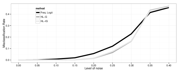
Figure 1: Results on Simulated A2 Matrices with different levels of noise - rank $3$

6.2 Real Data set: MovieLens

The last experiment involves the well known MovieLens data set. It has already been used by [13] and we follow them for the study. The ratings lie between $1$ to $5$ so we split them into binary data between good ratings (above the mean which is 3.5) and bad ones. The low rank assumption is usual in this case because it is expected that the taste of a particular user is related to only few hidden parameters. The smallest data set contains 100,000 ratings from 943 users and 1682 movies so we use 95,000 of them as a training set and the 5,000 remaining as the test set. The performances are very similar between the frequentist logistic model from [13] and the hinge loss model. The performances are slightly worse for the Bayesian logistic model so it is hard to favour a particular model at this stage.

Table 4: Performance rate on MovieLens 100k data set

Algorithm	HL-IG	HL-G	Logit-G	Logit-IG	Freq. Logit
correct classif. rate	.72	.71	.68	.68	.73

7 Discussion

We approach the 1-bit matrix completion problem with classification tools and it allows us to derive PAC-bounds on the risk. The previous works only focused on GLM models, which is not the right way to establish such risk bounds. This work relies on PAC-Bayesian framework and the pseudo-posterior distribution is approximated by a variational algorithm. In practice, it is able to deal with large matrices. We also derive a variational approximation of the posterior distribution in the Bayesian logistic model and it works very well in our examples.

The variational approximations look very promising in order to build algorithm which are able to deal with large data and this framework may be extended to more general models and other Machine Learning tools.

8 Proofs

8.1 Proofs of Proposition 1 from Section 2

Proof of Proposition 1.

Let $\rho=\rho_{L^{0},R^{0},v^{L},v^{R},\rho^{\gamma_{1}},\dots,\rho^{\gamma_{k}}}$ be a distribution from $\mathcal{F}$. The first term in (1) is upper bounded by the Lipschitz property of the hinge loss:

$$\int r_{n}^{h}(LR^{\top})\rho(dL,dR,d\gamma)=\frac{1}{n}\sum_{\ell=1}^{n}\int\left(1-Y_{\ell}L_{i_{\ell},\cdot}R_{j_{\ell},\cdot}^{\top}\right)_{+}\rho(dL,dR,d\gamma)$$

$$\leq\frac{1}{n}\sum_{\ell=1}^{n}\left(\left(1-Y_{\ell}L_{i_{\ell},\cdot}^{0}R_{j_{\ell},\cdot}^{0\top}\right)_{+}+\int|L_{i_{\ell},\cdot}R_{j_{\ell},\cdot}^{\top}-L_{i_{\ell},\cdot}^{0}R_{j_{\ell},\cdot}^{0\top}|\rho(dL,dR)\right)$$

$$\leq r_{n}^{h}\left(L^{0}R^{0\top}\right)+\frac{1}{n}\sum_{\ell=1}^{n}\sum_{k=1}^{K}\left[\sqrt{v^{L}_{i_{\ell},k}\frac{2}{\pi}}\sqrt{v^{R}_{j_{\ell},k}\frac{2}{\pi}}+|R_{j\ell,k}^{0}|\sqrt{v^{L}_{i_{\ell},k}\frac{2}{\pi}}+|L_{i_{\ell},k}^{0}|\sqrt{v^{R}_{j_{\ell},k}\frac{2}{\pi}}\right].$$

The second part (KL-divergence) can be explicitly calculated. Let $\rho^{L_{i,k}}$ denote the marginal distribution of $L_{i,k}$ under $\rho$. We define in the same way $\rho^{R_{j,k}}$. Also, $\pi\rho^{L_{i,k}|\gamma_{k}}$ denote the distribution of $L_{i,k}$ given $\gamma_{k}$ under $\pi$, and we define in the same way $\pi\rho^{R_{j,k}|\gamma_{k}}$. Then we have

$$\mathcal{K}(\rho,\pi) =\sum_{k=1}^{K}\left[\sum_{i=1}^{m_{1}}\mathbb{E}_{\rho^{\gamma_{k}}}\left[\mathcal{K}(\rho^{L_{i,k}},\pi^{L_{i,k}|\gamma_{k}})\right]+\sum_{j=1}^{m_{2}}\mathbb{E}_{\rho^{\gamma_{k}}}\left[\mathcal{K}(\rho^{R_{j,k}},\pi^{R_{j,k}|\gamma_{k}})\right]+\mathcal{K}(\rho^{\gamma_{k}},\pi^{\gamma_{k}})\right]$$

$$=\frac{1}{2}\sum_{k=1}^{K}\mathbb{E}_{\rho^{\gamma_{k}}}\left[\frac{1}{\gamma_{k}}\right]\left(\sum_{i=1}^{m_{1}}(v^{L}_{i,k}+L^{02}_{i,k})+\sum_{j=1}^{m_{2}}(v^{R}_{jk}+R^{02}_{j,k})\right)$$

$$-\frac{1}{2}\sum_{k=1}^{K}\left(\sum_{i=1}^{m_{1}}\log v^{L}_{i,k}+\sum_{j=1}^{m_{2}}\log v^{R}_{j,k}\right)+\sum_{k=1}^{K}\left[\mathcal{K}(\rho^{\gamma_{k}},\pi^{\gamma_{k}})+\frac{m_{1}+m_{2}}{2}\left(\mathbb{E}_{\rho^{\gamma_{k}}}\left[\log\gamma_{k}\right]-1\right)\right]$$

$$=\frac{1}{2}\sum_{k=1}^{K}\left[\sum_{i=1}^{m_{1}}\left(\mathbb{E}_{\rho^{\gamma_{k}}}\left[\frac{1}{\gamma_{k}}\right](v^{L}_{i,k}+L^{02}_{i,k})+\mathbb{E}_{\rho^{\gamma_{k}}}\left[\log\gamma_{k}\right]-\log v^{L}_{i,k}-1\right)\right.$$

$$\quad\left.+\sum_{j=1}^{m_{2}}\left(\mathbb{E}_{\rho^{\gamma_{k}}}\left[\frac{1}{\gamma_{k}}\right](v^{R}_{j,k}+R^{02}_{j,k})+\mathbb{E}_{\rho^{\gamma_{k}}}\left[\log\gamma_{k}\right]-\log v^{R}_{j,k}-1\right)+2\mathcal{K}(\rho^{\gamma_{k}},\pi^{\gamma_{k}})\right].$$

∎

8.2 Proofs of the results in Subsection 3.1

Proof of Theorem 1.

As the indicator function is uniformly bounded by $1$, we can use Lemma 5.1 in [1]:

$$\left.\begin{array}[]{l}\int\mathbb{E}\exp\{\lambda[R(LR^{\top})-r_{n}(LR^{\top})]\}{\rm d}\pi(R,L,\gamma)\\ \int\mathbb{E}\exp\{\lambda[r_{n}(LR^{\top})-R(LR^{\top})]\}{\rm d}\pi(R,L,\gamma)\end{array}\right\}\leq\exp\left[\frac{\lambda^{2}}{2n}\right].$$

So, the assumptions of Theorem 4.1 in [1] are satisfied and we obtain that, for any $\epsilon\in(0,1)$, with probability at least $1-\epsilon$ on the drawing of the sample, for any $\rho$ in $\mathcal{F}$:

$$\int Rd\rho \leq\int r_{n}d\rho+\frac{\mathcal{K}(\rho,\pi)}{\lambda}+\frac{\lambda}{2n}+\frac{\log\frac{1}{\epsilon}}{\lambda}$$

$$\leq\int r_{n}^{h}d\rho+\frac{\mathcal{K}(\rho,\pi)}{\lambda}+\frac{\lambda}{2n}+\frac{\log\frac{1}{\epsilon}}{\lambda}\text{ (as }r_{n}^{h}\geq r_{n}),$$

$$\leq r_{n}^{h}\left(L^{0}R^{0\top}\right)+\mathcal{R}(\rho,\lambda)+\frac{\lambda}{2n}+\frac{\log\frac{1}{\epsilon}}{\lambda}\text{ (thanks to Proposition~{}\ref{prop:VB_bound}).}$$

We end the proof by minimizing the right-hand-side w.r.t $\rho\in\mathcal{F}$. ∎

In order to prove Corollary 1, we need a preliminary result. For any $m_{1}\times m_{2}$ matrix $M$ with rank $r\in[K]$, we can write $M=LR^{T}$ where $L$ is $m_{1}\times K$, $R$ is $m_{2}\times K$ and, up to a reordering of the columns, $L_{\cdot,r+1}=\dots=L_{\cdot,K}=0$ and $R_{\cdot,r+1}=\dots=R_{\cdot,K}=0$. We denote by $\mathcal{B}(M)$ the set of such pairs of matrices $(L,R)$ and

$$\mathcal{F}(M)=\left\{\rho\in\mathcal{F}:(\mathbb{E}_{\rho}(L),\mathbb{E}_{\rho}(R))\in\mathcal{B}(M)\right\}.$$

Lemma 1.

There is a constant $\mathcal{C}_{\pi^{\gamma}}$ that depends only on the choice of the prior $\pi^{\gamma}$ such that for any $\lambda\leq n$,

$$\inf_{\rho\in\mathcal{F}(M)}\mathcal{R}(\rho,\lambda)\leq\mathcal{C}_{\pi^{\gamma}}\frac{{\rm rank}(M)(m_{1}+m_{2})(\ell(M)^{2}+\log n)}{\lambda},$$

$\mathcal{C}_{\pi^{\gamma}}$ is explicitly known and depends only on the choice of the prior $\pi^{\gamma}$ (Gamma, or Inverse-Gamma) and of its parameters.

It is obvious that when we combine Lemma 1 with Theorem 1 we obtain Corollary 1. It remains to prove the lemma.

Proof.

Let $M$ be fixed and for short let $r$ denote ${\rm rank}(M)$. We remind that, by definition:

$$\mathcal{R}(\rho,\lambda) =\frac{1}{n}\sum_{\ell=1}^{n}\sum_{k=1}^{K}\left[\sqrt{v^{L}_{i_{\ell},k}\frac{2}{\pi}}\sqrt{v^{R}_{j_{\ell},k}\frac{2}{\pi}}+|R_{j_{\ell},k}^{0}|\sqrt{v^{L}_{i_{\ell},k}\frac{2}{\pi}}+|L_{i_{\ell},k}^{0}|\sqrt{v^{R}_{j_{\ell},k}\frac{2}{\pi}}\right]$$

$$+\frac{1}{\lambda}\left(\frac{1}{2}\sum_{k=1}^{K}\mathbb{E}_{\rho}\left[\frac{1}{\gamma_{k}}\right]\left(\sum_{i=1}^{m_{1}}(v^{L}_{ik}+L^{02}_{ik})+\sum_{j=1}^{m_{2}}(v^{R}_{jk}+R^{02}_{jk})\right)-\frac{1}{2}\sum_{k=1}^{K}\left(\sum_{i=1}^{m_{1}}\log v^{L}_{ik}+\sum_{j=1}^{m_{2}}\log v^{R}_{jk}\right)\right.$$

$$\left.+\sum_{k=1}^{K}\left[\mathcal{K}(\rho^{\gamma_{k}},\pi^{\gamma})+\frac{m_{1}+m_{2}}{2}\left(\mathbb{E}_{\rho}\left[\log\gamma_{k}\right]-1\right)\right]\right).$$

We will now upper bound the infimum for a special choice for $\rho=\rho_{L^{0},R^{0},v^{L},v^{R},\rho^{\gamma_{1}},\dots,\rho^{\gamma_{k}}}$ with $(L^{0},R^{0})\in\mathcal{B}(M)$: for all pairs $(i,k)$ and $(j,k^{\prime})$ $v_{i,k}^{L}=v_{j,k}^{R}=v^{0}$ when $k,k^{\prime}\leq r$ $v_{i,k}^{L}=v_{j,k}^{R}=v^{1}$ otherwise. The choice for $v^{0}$ and $v^{1}$ will be given below. For $\gamma$, we fix two distributions $\rho_{\gamma}^{0}$ and $\rho_{\gamma}^{1}$ and fix $\rho^{\gamma_{k}}=\rho_{\gamma}^{0}$ for $k\leq r$ and $\rho^{\gamma_{k}}=\rho_{\gamma}^{1}$ otherwise. Then:

$$\inf_{\rho\in\mathcal{F}(M)}\mathcal{R}(\rho,\lambda) \leq\frac{2}{\pi}((K-r)v^{1}+rv_{0})+2r\ell(M)\sqrt{\frac{2v^{0}}{\pi}}+\frac{1}{\lambda}\left(r\mathcal{K}(\rho_{\gamma}^{0},\pi^{\gamma})+(K-r)\mathcal{K}(\rho_{\gamma}^{1},\pi^{\gamma})\right)$$

$$\quad+\frac{m_{1}+m_{2}}{2\lambda}\Biggl{\{}r\underbrace{\left[\mathbb{E}_{\rho^{0}_{\gamma}}\left[\frac{1}{\gamma_{k}}\right](v^{0}+\ell^{2}(M))+\mathbb{E}_{\rho^{0}_{\gamma}}\log\gamma_{k}-\log v^{0}-1\right]}_{A_{1}}$$

$$+(K-r)\underbrace{\left[\mathbb{E}_{\rho^{1}_{\gamma}}\left[\frac{1}{\gamma_{k}}\right]v_{1}+\mathbb{E}_{\rho^{0}_{\gamma}}\log\gamma_{k}-\log v^{1}-1\right]}_{A_{2}}\Biggr{\}}.$$

By actually choosing $\rho_{\gamma}^{0}=\pi^{\gamma}|_{[1,1+\delta]}$ for some $\delta>0$ and $\rho_{\gamma}^{1}=\pi^{\gamma}|_{[v^{1},v_{1}+\delta]}$, we obtain

$$A_{2} \leq 1-1+\log\frac{v^{1}+\delta}{v^{1}}\leq\frac{\delta}{v^{1}};$$

$$A_{1} \leq v^{0}+l^{2}+\delta-\log v^{0}.$$

At this stage, we can set the free parameters $v_{0}$, $v_{1}$ and $\delta$ in order to reach the desired rate. The choices are: $v_{1}=\frac{1}{n},v_{0}=\frac{1}{n^{2}},\delta=\frac{r}{Kn}$. We finally have to upper bound $r\mathcal{K}(\rho_{\gamma}^{0},\pi^{\gamma})+(K-r)\mathcal{K}(\rho_{\gamma}^{1},\pi^{\gamma})$. The upper bound actually depends on the choice for $\pi^{\gamma}$. We consider three cases: the Gamma prior with $\alpha\geq 1$, with $\alpha<1$ and then the inverse-Gamma prior.

Let us deal with the $\Gamma^{-1}(\alpha,\beta)$ prior first:

$$r\mathcal{K}(\rho_{\gamma}^{0},\pi^{\gamma})+(K-r)\mathcal{K}(\rho_{\gamma}^{1},\pi^{\gamma})-K\log\frac{1}{\delta}-K\log\frac{\Gamma(\alpha)}{\beta^{\alpha}}$$

$$\leq r[(\alpha+1)\log(1+\delta)+\beta]+(K-r)[(\alpha+1)\log(v_{1}+\delta)+\frac{\beta}{v_{1}}]$$

$$\leq r[(\alpha+1)\delta+\beta]+(K-r)\left[(\alpha+1)(\log v_{1}+\frac{\delta}{v_{1}})+\frac{\beta}{v_{1}}\right]$$

$$\leq r[(\alpha+1)\frac{r}{Kn}+\beta]+K\left[(\alpha+1)(-\log n+1)+n\beta\right]$$

Let’s turn to the $\Gamma(\alpha,\beta)$ distribution with $\alpha\geq 1$:

$$r\mathcal{K}(\rho_{\gamma}^{0},\pi^{\gamma})+(K-r)\mathcal{K}(\rho_{\gamma}^{1},\pi^{\gamma})-K\log\frac{1}{\delta}-K\log\frac{\Gamma(\alpha)}{\beta^{\alpha}}$$

$$\leq r[\beta(1+\delta)]+(K-r)[-(\alpha-1)\log v_{1}+\beta(v_{1}+\delta)]$$

$$\leq r[\beta(1+\delta)]+(K-r)[(\alpha-1)\log\frac{1}{v_{1}}+\beta(v_{1}+\delta)]$$

$$\leq 2r\beta+K[(\alpha-1)\log n+\frac{2\beta}{n}]$$

The last case is the $\Gamma(\alpha,\beta)$ distribution with $0<\alpha<1$:

$$r\mathcal{K}(\rho_{\gamma}^{0},\pi^{\gamma})+(K-r)\mathcal{K}(\rho_{\gamma}^{1},\pi^{\gamma})-K\log\frac{1}{\delta}-K\log\frac{\Gamma(\alpha)}{\beta^{\alpha}}$$

$$\leq r[-(\alpha-1)\log(1+\delta)+\beta(1+\delta)]+(K-r)[-(\alpha-1)\log(v_{1}+\delta)+\beta(v_{1}+\delta)]$$

$$\leq r[(1-\alpha)\delta+\beta(1+\delta)]+(K-r)[(1-\alpha)(\log v_{1}+\frac{\delta}{v_{1}})+\beta(v_{1}+\delta)]$$

$$\leq 2r\beta+r(1-\alpha)\frac{r}{Kn}+K[(1-\alpha)(-\log n+1)+\frac{2\beta}{n}]$$

In any case, as $\lambda\leq n$, when $\alpha$ and $\beta$ are constant, the leading term is in $\frac{r(m_{1}+m_{2})(\ell^{2}(M)+\log n)}{\lambda}$ so we can upper bound the whole by $\mathcal{C}_{\pi^{\gamma}}\frac{r(m_{1}+m_{2})(\ell^{2}(M)+\log n)}{\lambda}$ where $\mathcal{C}_{\pi^{\gamma}}$ depends on $\alpha$ and $\beta$ (and takes a different form depending on the case: Gamma or inverse-Gamma). ∎

Note actually that from the previous proof we can provide more explicit forms for the bound in the three cases. We did not include this in the core of the paper, but we prove the following lemmas for the sake of completeness.

Lemma 2.

When $\pi^{\gamma}=\Gamma(\alpha,\beta)$,

$$\inf_{\rho\in\mathcal{F}(M)}\mathcal{R}(\rho,\lambda) \leq\frac{1}{n}\left[\frac{4}{\pi}K+\sqrt{\frac{8}{\pi}}r\ell(M)\right]+\frac{r(m_{1}+m_{2})}{2\lambda}\left[3+\ell^{2}(M)+2\log n\right]$$

$$\quad+\frac{K}{\lambda}\left[\log\frac{Kn}{r}+\log\frac{\Gamma(\alpha)}{\beta^{\alpha}}+\frac{r}{K}\left[(\alpha+1)\frac{r}{Kn}+\beta\right]+\left[(\alpha+1)(-\log n+1)+n\beta\right]\right].$$

Lemma 3.

When $\pi^{\gamma}=\Gamma^{-1}(\alpha,\beta)$ with $\alpha\geq 1$,

$$\inf_{\rho\in\mathcal{F}(M)}\mathcal{R}(\rho,\lambda) \leq\frac{1}{n}\left[\frac{4}{\pi}K+\sqrt{\frac{8}{\pi}}r\ell(M)\right]+\frac{r(m_{1}+m_{2})}{2\lambda}\left[3+\ell^{2}(M)+2\log n\right]$$

$$\quad+\frac{K}{\lambda}\left[\log\frac{Kn}{r}+\log\frac{\Gamma(\alpha)}{\beta^{\alpha}}+\frac{2r\beta}{K}+\left[(\alpha-1)\log n+\frac{2\beta}{n}\right]\right].$$

Lemma 4.

When $\pi^{\gamma}=\Gamma^{-1}(\alpha,\beta)$ with $0<\alpha<1$,

$$\inf_{\rho\in\mathcal{F}(M)}\mathcal{R}(\rho,\lambda) \leq\frac{1}{n}\left[\frac{4}{\pi}K+\sqrt{\frac{8}{\pi}}r\ell(M)\right]+\frac{r(m_{1}+m_{2})}{2\lambda}\left[3+\ell^{2}(M)+2\log n\right]$$

$$\quad+\frac{K}{\lambda}\left[\log\frac{Kn}{r}+\log\frac{\Gamma(\alpha)}{\beta^{\alpha}}+\frac{2r\beta}{K}+(1-\alpha)\frac{r^{2}}{K^{2}n}+\left[(1-\alpha)(-\log n+1)+\frac{2\beta}{n}\right]\right].$$

8.3 Proofs of the results in Subsection 3.2

We first start with preliminary lemmas.

Lemma 5.

For $\epsilon>0$, with probability at least $1-\epsilon$ and for every $s\in(0,1)$,

$$\overline{r_{n}}\leq(1+s)\overline{R}+\frac{1}{ns}\log\frac{1}{\epsilon}$$

Proof.

Let $s\in(0,1)$, then

$$\mathbb{E}\left(\exp[sn\overline{r_{n}}]\right) =\prod_{\ell=1}^{n}\mathbb{E}\left(\exp\left[s\mathbbm{1}(Y_{\ell}M^{B}_{X_{\ell}}<0)\right]\right)$$

$$=\prod_{\ell=1}^{n}\mathbb{E}\left(\exp\left[s\mathbbm{1}(Y_{\ell}M^{B}_{X_{\ell}}<0)+0\left(1-\mathbbm{1}(Y_{\ell}M^{B}_{X_{\ell}}<0)\right)\right]\right)$$

$$\leq\prod_{\ell=1}^{n}\left(\left(1-\mathbb{E}\left[\mathbbm{1}(Y_{\ell}M^{B}_{X_{\ell}}<0)\right]\right)+e^{s}\mathbb{E}\left[\mathbbm{1}(Y_{\ell}M^{B}_{X_{\ell}}<0)\right]\right)$$

$$\leq\prod_{\ell=1}^{n}\left((1-\overline{R})+e^{s}\overline{R}\right)=\prod_{\ell=1}^{n}\left(1+\overline{R}(e^{s}-1)\right)$$

$$\leq\prod_{\ell=1}^{n}\exp\left(\overline{R}(e^{s}-1)\right)=\exp\left(n\overline{R}(e^{s}-1)\right).$$

Therefore, for $\epsilon\in(0,1)$:

$$\mathbb{E}\left[\exp\left(sn\overline{r_{n}}-n\overline{R}(e^{s}-1)-\log\frac{1}{\epsilon}\right)\right]\leq\epsilon.$$

We use the fact that $\mathbb{E}[\exp U]\geq\mathbb{P}(U>0)$ (Markov’s inequality) for any $U$ so, with probability at least $1-\epsilon$:

$$\overline{r_{n}}\leq\frac{e^{s}-1}{s}\overline{R}+\frac{\log\frac{1}{\epsilon}}{sn}$$

On $[0,1]$, $e^{x}\leq 1+x+x^{2}$ so it’s done. ∎

Lemma 6.

Assume that Mammen and Tsybakov’s assumption is satisfied for a certain constant $C$. Assume that $\lambda<2n/C$. Then, for $\epsilon>0$, with probability at least $1-\epsilon$:

$$\int Rd\widetilde{\rho}_{\lambda}\leq\overline{R}+\frac{1}{1-C\lambda/(2n)}\left\{\inf_{\rho\in\mathcal{F}}\left[r_{n}^{h}\left(L^{0}R^{0\top}\right)+\mathcal{R}(\rho,\lambda)\right]-\overline{r}_{n}+\frac{1}{\lambda}\log\left(\frac{1}{\epsilon}\right)\right\}$$ (6)

Proof.

Assume that the Mammen and Tsybakov’s assumption is satisfied for a certain constant C. The $0-1$ loss is bounded then, from Bernstein’s inequality (Theorem 10 page 37 in [3]) we get:

$$\int\mathbb{E}\exp\{\lambda[R(LR^{\top})-\overline{R}]-\lambda[r_{n}(LR^{\top})-\overline{r}_{n}]\}{\rm d}\pi(L,R,\gamma)\leq\int\exp[C\lambda^{2}/(2n)[R(LR^{\top})-\overline{R}]]{\rm d}\pi(L,R,\gamma).$$

Apply Fubini’s theorem to the inequality:

$$\mathbb{E}\int\exp\{(\lambda-C\lambda^{2}/(2n))[R(LR^{\top})-\overline{R}]-\lambda[r_{n}(LR^{\top})-\overline{r}_{n}]\})\pi(d\theta)\leq 1$$

(we remind that $\theta=(L,R,\gamma)$ for short).

$$\mathbb{E}\exp\left\{\sup_{\rho}\int[\lambda[R(LR^{\top})-\overline{R}]-\lambda[r_{n}(LR^{\top})-\overline{r}_{n}]-C\lambda^{2}/(2n)[R(LR^{\top})-\overline{R}]]\rho(d\theta)-\mathcal{K}(\rho,\pi)\right\}\leq 1.$$

Using Markov’s inequality,

$$\mathbb{P}\left(\sup_{\rho}\int[(\lambda-C\lambda^{2}/(2n))[R(LR^{\top})-\overline{R}]-\lambda[r_{n}(LR^{\top})-\overline{r}_{n}]]\rho(d\theta)-\mathcal{K}(\rho,\pi)+\log\epsilon>0\right)\leq\epsilon.$$

Then take the complementary of this event and we get that with probability at least $1-\epsilon$:

$$\forall\rho,\qquad(\lambda-C\lambda^{2}/(2n))\int[R(LR^{\top})-\overline{R}]\rho(d\theta)\leq\lambda\int[r_{n}(LR^{\top})-\overline{r}_{n}]\rho(d\theta)+\mathcal{K}(\rho,\pi)+\log\frac{1}{\epsilon}$$

Now, note that

$$(\lambda-C\lambda^{2}/(2n))\left[\int Rd\rho-\overline{R}\right] \leq\lambda\left[\int r_{n}d\rho-\overline{r}_{n}\right]+\mathcal{K}(\rho,\pi)+\log\left(\frac{1}{\epsilon}\right)$$

$$\Rightarrow(\lambda-C\lambda^{2}/(2n))\left[\int Rd\rho-\overline{R}\right] \leq\lambda\left[\int r_{n}^{h}d\rho+\frac{1}{\lambda}\mathcal{K}(\rho,\pi)\right]-\lambda\overline{r}_{n}+\log\left(\frac{1}{\epsilon}\right)$$

$$\Rightarrow(\lambda-C\lambda^{2}/(2n))\left[\int Rd\rho-\overline{R}\right] \leq\lambda\left[r_{n}^{h}\left(L^{0}R^{0\top}\right)+\mathcal{R}(\rho,\lambda)-\overline{r}_{n}+\frac{1}{\lambda}\log\left(\frac{1}{\epsilon}\right)\right]$$

As it stands for all $\rho$ then the right hand side can be minimized and the minimizer over $\mathcal{F}$ is $\widetilde{\rho}_{\lambda}$. Thus we get, when $\lambda<2n/C$,

$$\int Rd\widetilde{\rho}_{\lambda}\leq\overline{R}+\frac{1}{1-C\lambda/(2n)}\left\{\inf_{\rho\in\mathcal{F}}\left[r_{n}^{h}\left(L^{0}R^{0\top}\right)+\mathcal{R}(\rho,\lambda)\right]-\overline{r}_{n}+\frac{1}{\lambda}\log\left(\frac{1}{\epsilon}\right)\right\}$$

∎

We are now ready for the proofs.

Proof of Theorem 2.

We apply Lemma 6 and, as we have $\mathcal{F}(M^{B})\subset\mathcal{F}$,

$$\int Rd\widetilde{\rho}_{\lambda}\leq\overline{R}+\frac{1}{1-C\lambda/(2n)}\left\{\inf_{\rho\in\mathcal{F}(M)}\left[r_{n}^{h}\left(L^{0}R^{0\top}\right)+\mathcal{R}(\rho,\lambda)\right]-\overline{r}_{n}+\frac{1}{\lambda}\log\left(\frac{1}{\epsilon}\right)\right\}$$ (7)

As by definition, all the entries of $M^{B}$ are in $\{-1,1\}$, $r_{n}^{h}(M^{B})=2\overline{r_{n}}$ and then, by Lemma 1:

$$\int Rd\widetilde{\rho}_{\lambda}\leq\overline{R}+\frac{1}{1-C\lambda/(2n)}\left\{2\overline{r_{n}}+\mathcal{C}_{\pi^{\gamma}}\frac{{\rm rank}(M^{B})(m_{1}+m_{2})(\ell^{2}(M)+\log n)}{\lambda}+\frac{1}{\lambda}\log\left(\frac{1}{\epsilon}\right)\right\}$$

Then, we use Lemma 6 to get, with probability at least $1-2\varepsilon$,

$$\int Rd\widetilde{\rho}_{\lambda} \leq\overline{R}+\frac{1}{1-C\lambda/(2n)}\Biggl{\{}2(1+s)\overline{R}+\frac{1}{ns}\log\frac{1}{\epsilon}$$

$$+\mathcal{C}_{\pi^{\gamma}}\frac{{\rm rank}(M^{B})(m_{1}+m_{2})(\ell^{2}(M)+\log n)}{\lambda}+\frac{1}{\lambda}\log\left(\frac{1}{\epsilon}\right)\Biggr{\}}$$

To end up the proof, we have to take $\lambda=\frac{2cn}{C}$ with $c\in(0,1/2)$. We thus have:

$$\frac{1}{1-C\lambda/(2n)}=\frac{1}{1-c}\leq 1+2c,$$

this ends the proof by taking $c=s/2$. ∎

Proof of Corollary 2.

As we are in the noiseless case, the margin assumption is satisfied with $C=1$, and $\overline{R}=0$. ∎

8.4 Detailed calculations for Subsection 5

Proof of Proposition 2.

From [15], we have the following lower bound:

$$\forall(x,\xi)\in\mathbb{R}^{2}$$

$$\log\sigma(x)\geq\log\sigma(\xi)+\frac{x-\xi}{2}-\tau(\xi)(x^{2}-\xi^{2})\quad\textrm{where}\quad\tau(\xi)=\frac{1}{2\xi}\left(\sigma(\xi)-\frac{1}{2}\right)$$

The likelihood of one observation $y\in\{-1,1\}$ at point $x$ is then lower bounded:

$$\forall\xi\in\mathbb{R},\sigma(yx) \geq\sigma(\xi)\exp\left\{\frac{yx-\xi}{2}-\tau(\xi)(x^{2}-\xi^{2})\right\}:=h(yx,\xi).$$

Therefore, the likelihood of the model is lower bounded:

$$\forall\xi\in\mathbb{R}^{n},\quad\Lambda(L,R) =\prod_{l=1}^{n}\sigma(Y_{l}(LR^{\top})_{X_{l}})$$

$$\geq\prod_{l=1}^{n}\sigma(\xi_{l})\exp\left\{\frac{(LR^{\top})_{X_{l}}-\xi_{l}}{2}-\tau(\xi_{l})\left[(LR^{\top})_{X_{l}}^{2}-\xi_{l}^{2}\right]\right\}:=H(\theta,\xi).$$

∎

It is now easy to optimize $\mathcal{L}(\rho,\xi)$ with respect to $\xi$ elementwise, which is the same as maximizing $H(\theta,\xi)$ elementwise and then each part $h(Y_{l}(LR^{\top})_{X_{l}},\xi_{l})$:

$$\widehat{\xi_{l}} =\textrm{arg}\max_{\xi_{l}}\int\log H(\theta,\xi)\rho(d\theta)=\textrm{arg}\max_{\xi_{l}}\mathbb{E}_{\rho}\left[\log h(Y_{l}(LR^{\top})_{X_{l}},\xi_{l})\right]$$

$$=\textrm{arg}\max_{\xi_{l}}\left\{\log\sigma(\xi_{l})-\frac{\xi_{l}}{2}-\tau(\xi_{l})\left(\mathbb{E}_{\rho}\left[(LR^{\top})_{X_{l}}^{2}\right]-\xi_{ij}^{2}\right)\right\}$$

The maximum is reached at the zero of the derivative and we can conclude that:

$$\widehat{\xi_{l}}^{2} =\mathbb{E}_{\rho}\left[(LR^{\top})_{X_{l}}^{2}\right]$$

References

• [1] P. Alquier, J. Ridgway, and N. Chopin. On the properties of variational approximations of Gibbs posteriors. ArXiv e-prints, June 2015.
• [2] C. M. Bishop. Pattern Recognition and Machine Learning (Information Science and Statistics). Springer-Verlag New York, Inc., Secaucus, NJ, USA, 2006.
• [3] S. Boucheron, G. Lugosi, and P. Massart. Concentration inequalities: A nonasymptotic theory of independence. OUP Oxford, 2013.
• [4] S. Boyd, N. Parikh, E. Chu, B. Peleato, and J. Eckstein. Distributed optimization and statistical learning via the alternating direction method of multipliers. Foundations and Trends in Machine Learning, 3(1):1–122, 2011.
• [5] T. Cai and W.-X. Zhou. A max-norm constrained minimization approach to 1-bit matrix completion. Journal of Machine Learning Research, 14:3619–3647, 2013.
• [6] E. J. Candès and Y. Plan. Matrix Completion With Noise. Proceedings of the IEEE, 98(6):925–936, 2010.
• [7] E. J. Candès and B. Recht. Exact matrix completion via convex optimization. Commun. ACM, 55(6):111–119, 2012.
• [8] E. J. Candès and T. Tao. The power of convex relaxation: near-optimal matrix completion. IEEE Transactions on Information Theory, 56(5):2053–2080, 2010.
• [9] O. Catoni. Statistical Learning Theory and Stochastic Optimization. Saint-Flour Summer School on Probability Theory 2001 (Jean Picard ed.), Lecture Notes in Mathematics. Springer, 2004.
• [10] O. Catoni. PAC-Bayesian supervised classification: the thermodynamics of statistical learning. Institute of Mathematical Statistics Lecture Notes—Monograph Series, 56. Institute of Mathematical Statistics, Beachwood, OH, 2007.
• [11] S. Chatterjee. Matrix estimation by universal singular value thresholding. Ann. Statist., 43(1):177–214, 02 2015.
• [12] A. Dalalyan and A. B. Tsybakov. Aggregation by exponential weighting, sharp PAC-Bayesian bounds and sparsity. Machine Learning, 72(1):39–61, 2008.
• [13] M. A. Davenport, Y. Plan, E. van den Berg, and M. Wootters. 1-Bit Matrix Completion. to appear in Information and Inference, 2014.
• [14] R. Herbrich and T. Graepel. A PAC-Bayesian margin bound for linear classifiers. IEEE Transactions on Information Theory, 48(12):3140–3150, 2002.
• [15] T. S. Jaakkola and M. I. Jordan. Bayesian parameter estimation via variational methods. Statistics and Computing, 10(1):25–37, 2000.
• [16] O. Klopp, J. Lafond, E. Moulines, and J. Salmon. Adaptive Multinomial Matrix Completion. ArXiv e-prints, August 2014.
• [17] M. Kyung, J. Gill, M. Ghosh, and G. Casella. Penalized regression, standard errors, and Bayesian lassos. Bayesian Analysis, 5(2):369–412, 2010.
• [18] Pierre Latouche, Stéphane Robin, and Sarah Ouadah. Goodness of fit of logistic models for random graphs. arXiv preprint arXiv:1508.00286, 2015.
• [19] Y. J. Lim and Y. W. Teh. Variational Bayesian approach to movie rating prediction. In Proceedings of KDD Cup and Workshop, 2007.
• [20] T. T. Mai and P. Alquier. A bayesian approach for noisy matrix completion: Optimal rate under general sampling distribution. Electron. J. Statist., 9(1):823–841, 2015.
• [21] E. Mammen and A. Tsybakov. Smooth discrimination analysis. The Annals of Statistics, 27(6):1808–1829, 1999.
• [22] D.A. McAllester. Some PAC-Bayesian theorems. In Proceedings of the Eleventh Annual Conference on Computational Learning Theory, pages 230–234, New York, 1998. ACM.
• [23] T. Park and G. Casella. The Bayesian Lasso. Journal of the American Statistical Association, 103(482):681–686, 2008.
• [24] B. Recht and C. Ré. Parallel stochastic gradient algorithms for large-scale matrix completion. Mathematical Programming Computation, 5(2):201–226, 2013.
• [25] R. Salakhutdinov and A. Mnih. Bayesian probabilistic matrix factorization using Markov chain Monte Carlo. In Proceedings of the 25th International Conference on Machine Learning, pages 880–887, 2008.
• [26] Y. Seldin, F. Laviolette, N. Cesa-Bianchi, J. Shawe-Taylor, and P. Auer. PAC-Bayesian inequalities for martingales. IEEE Transactions on Information Theory, 58(12):7086–7093, 2012.
• [27] J. Shawe-Taylor and J. Langford. PAC-Bayes & margins. Advances in neural information processing systems, 15:439, 2003.
• [28] N. Srebro, J. Rennie, and T. S. Jaakkola. Maximum-margin matrix factorization. In Advances in neural information processing systems, pages 1329–1336, 2004.
• [29] V. Vapnik. Statistical Learning Theory. Wiley, 1998.
• [30] T. Zhang. Statistical behavior and consistency of classification methods based on convex risk minimization. Ann. Statist., 32(1):56–85, 02 2004.