Loss of solution in the symmetry improved $\Phi$-derivable expansion scheme

Abstract

We consider the two-loop $\Phi$-derivable approximation for the $O(2)$-symmetric scalar model, augmented by the symmetry improvement introduced in Pilaftsis and Teresi (2013) [9], which enforces Goldstone’s theorem in the broken phase. Although the corresponding equations admit a solution in the presence of a large enough infrared (IR) regulating scale, we argue that, for smooth ultraviolet (UV) regulators, the solution is lost when the IR scale becomes small enough. Infrared regular solutions exist for certain non-analytic UV regulators, but we argue that these solutions are artifacts which should disappear when the sensitivity to the UV regulator is removed by a renormalization procedure. The loss of solution is observed both at zero and at finite temperature, although it is simpler to identify in the latter case. We also comment on possible ways to cure this problem.

1 Introduction

The two-particle-irreducible ($2$PI) effective action formalism and the corresponding $\Phi$-derivable expansion scheme are appropriate to study the dynamical evolution of far from equilibrium quantum systems [1] and some of their equilibrium properties [2, 3, 4, 5]. Despite their many applications, they suffer, however, from a major problem in the case of a spontaneously broken continuous symmetry: Goldstone’s theorem is violated by the approximations which casts a doubt on the obtained physical results. Recently, some approaches have been put forward to correct for this problem, but they are either restricted to specific approximations [6, 7] or they require a non-linear representation of the degrees of freedom [8], which makes the practical implementation difficult. More recently, a systematic approach based on the usual linear representation of the fields has been proposed by Pilaftsis and Teresi [9] and applied to various situations of interest [10, 11, 12].

In this paper we discuss this latter approach, the so-called symmetry improvement, in its application to the O($2$)-symmetric scalar model at two-loop level, as in [9]. We argue that, although the corresponding equations are formally compatible with Goldstone’s theorem in the absence of an IR regulating scale (“infinite volume”), they do not have a physical solution (in fact they do not have a physical solution for a small enough IR scale, that is for a “large enough volume”), if the UV regulator is chosen smooth enough. Infinite volume solutions can be found for certain non-analytic UV regulators and for a fixed value of the cutoff. Even though these solutions could be of relevance in cases where such UV regulators have a physical origin, we argue that they should be regarded as artifacts in applications where the UV regulator has not such origin and that they should in principle disappear when the dependence with respect to the UV regulator is eventually removed by a renormalization procedure. We believe that the absence of infinite volume solutions manifests itself in other truncations or models when the symmetry improvement is considered. It illustrates the fact that it may not be enough to overimpose Goldstone’s theorem in order to solve the above mentioned problem of the $\Phi$-derivable scheme. One might need, in addition, to make sure that the considered truncation can cope dynamically (and not just fictitiously through some non-analyticity of the UV regulator) with the infrared sensitivity that the presence of Goldstone modes entails.

The implications of the results reported in this paper concerning the fate of the symmetry improvement should not be considered as definitive, because we cannot give a complete analytical proof of the loss of solution. We can only illustrate it using semi-rigorous analytical arguments, supported by a numerical investigation which, although compelling, is based on methods that possess their own limitations. Nevertheless, we believe that in the two-loop approximation considered in [9], the original formulation of the symmetry improvement faces problems related to infrared sensitivity. Our purpose is then to initiate some discussion on this recently proposed approach that we believe is interesting but calls, in our view, for some critical discussion. In fact, we have briefly reported on the loss of solution at finite temperature in Sec. V.C of [13]. In the present paper, we would like to provide a more thorough investigation including the $T=0$ case as well.

In Sec. 2, we present the two-loop $\Phi$-derivable equations in the symmetry improved approach and give a semi-rigorous argument in favor of the absence of infinite volume solutions. We then support this claim with a numerical investigation, first at $T=0$ in Sec. 3 and then at finite $T$ in Sec. 4. We finally discuss possible ways to circumvent the problem.

2 The symmetry improved two-loop $\Phi$-derivable approximation

2.1 Equations

In the standard two-loop $\Phi$-derivable approximation of the $O(2)$-symmetric scalar model, see e.g. [15], the so-called gap equations for a fixed value of the field expectation value $\phi$ (in the presence of a uniform source) are given by

$$\bar{M}^{2}_{\rm L}(K) = m^{2}_{0}+\frac{\lambda_{0}^{(A+2B)}}{12}{\mathcal{T}}[\bar{G}_{\rm L}]+\frac{\lambda^{(A)}_{0}}{12}{\mathcal{T}}[\bar{G}_{\rm T}]$$ (1)

$$+ \phi^{2}\left[\frac{\lambda_{2}^{(A+2B)}}{12}-\frac{\lambda^{2}}{72}\big{(}9{\mathcal{B}}[\bar{G}_{\rm L}](K)+{\mathcal{B}}[\bar{G}_{\rm T}](K)\big{)}\right],$$

$$\bar{M}^{2}_{\rm T}(K) = m^{2}_{0}+\frac{\lambda_{0}^{(A)}}{12}{\mathcal{T}}[\bar{G}_{\rm L}]+\frac{\lambda^{(A+2B)}_{0}}{12}{\mathcal{T}}[\bar{G}_{\rm T}]+\phi^{2}\left[\frac{\lambda^{(A)}_{2}}{12}-\frac{\lambda^{2}}{36}{\cal B}[\bar{G}_{\rm L};\bar{G}_{\rm T}](K)\right],$$ (2)

where $\bar{M}^{2}_{\rm L}(K)$ and $\bar{M}^{2}_{\rm T}(K)$ are the momentum dependent squared gap masses, related to the propagators by

$$\bar{G}_{\text{L,T}}(K)=\frac{1}{K^{2}+\bar{M}^{2}_{\text{L,T}}(K)}\,.$$ (3)

The bare mass $m_{0}$ and the various bare couplings $\lambda_{0}^{(A)}$, $\lambda_{0}^{(B)}$, $\lambda_{2}^{(A)}$ and $\lambda_{2}^{(B)}$ are required for renormalization and $\lambda$ is the renormalized coupling, see the discussion below and in [16, 17, 15, 18]. We have introduced the short-hand notations

$$\lambda_{i}^{(\alpha A+\beta B)}\equiv\alpha\lambda_{i}^{(A)}+\beta\lambda_{i}^{(B)}\,,$$ (4)

with $i=0$ or $2$, as well as

$${\mathcal{T}}[G] \equiv \int_{Q}^{T}G(Q)\,,$$ (5)

$${\mathcal{B}}[G_{1};G_{2}](K) \equiv \int_{Q}^{T}G_{1}(Q)G_{2}(Q+K)\,,$$ (6)

for the tadpole and bubble integrals, where

$$\int_{Q}^{T}f(Q)\equiv T\sum_{n=-\infty}^{\infty}\int\frac{d^{3}q}{(2\pi)^{3}}f(i\omega_{n},{\bm{q}})\,.$$ (7)

It is also understood that whenever $\smash{G_{1}=G_{2}}$, we shall write more simply ${\mathcal{B}}[G_{1};G_{1}](K)={\mathcal{B}}[G_{1}](K)$. We shall also denote ${\mathcal{B}}[G_{1};G_{2}](\smash{K=0})$ more simply as ${\mathcal{B}}[G_{1};G_{2}]$.

The field-dependent propagators $\bar{G}_{\text{L,T}}$ allow us to construct the effective potential, the extrema of which are given in terms of the so-called field equation. As we recalled in the Introduction, a well known problem of the standard $\Phi$-derivable approach is that, in the broken phase, the transverse propagator $\bar{G}_{\mathrm{T}}$ evaluated at the minimum $\bar{\phi}$ of the potential does not fulfill Goldstone’s theorem. In the approach recently proposed by Pilaftsis and Teresi [9], the field equation (in the broken phase) is replaced by the constraint $\bar{M}^{2}_{\mathrm{T}}(0)=0$. This constraint, together with (2) can then be rewritten as

$$\bar{M}^{2}_{\rm T}(K) = -\frac{\lambda^{2}}{36}\bar{\phi}^{2}\Big{[}{\mathcal{B}}[\bar{G}_{\rm L};\bar{G}_{\rm T}](K)-{\mathcal{B}}[\bar{G}_{\rm L};\bar{G}_{\rm T}]\Big{]}\,,$$ (8)

$$\bar{\phi}^{2} = -\frac{\displaystyle m^{2}_{0}+\frac{\lambda_{0}^{(A)}}{12}{\mathcal{T}}[\bar{G}_{\rm L}]+\frac{\lambda^{(A+2B)}_{0}}{12}{\mathcal{T}}[\bar{G}_{\rm T}]}{\displaystyle\frac{\lambda^{(A)}_{2}}{12}-\frac{\lambda^{2}}{36}{\mathcal{B}}[\bar{G}_{\rm L};\bar{G}_{\rm T}]}\,,$$ (9)

while the equation (1) for $\bar{M}^{2}_{\mathrm{L}}$ remains the same, apart from the change $\phi^{2}\to\bar{\phi}^{2}$.

Goldstone’s theorem seems thus to be obeyed by construction. However this is only true if the system of equations (1), (8) and (9) admits a solution. As we now argue and as we illustrate in the next sections, we believe that the above equations do not have a solution.

2.2 A tentative argument supporting the absence of solutions

Let us first mention that systems of equations such as (1) and (2), or (1), (8) and (9) are known to have no solution if they are not properly UV regularized [19]. Thus, in what follows, we assume that we have chosen some UV regularization of the sum-integrals $\mathcal{T}$ and ${\mathcal{B}}$, to which an UV scale or cutoff $\Lambda$ is associated. For definiteness, we restrict to regularizations such that each propagator $\bar{G}_{\mathrm{L,T}}(Q)$ that enters an integral is multiplied by a certain regulating function $R(x)$, with $x=Q/\Lambda$ in the $T=0$ case or $x=q/\Lambda$ in the $T\neq 0$ case, but of course, for the applications that we have in mind, the final results should not depend (or depend as less as possible) on the choice of the UV regulator. We shall come back to this point below.

We shall first consider the case of smooth enough UV regulators. In this case, our argument will already exclude the existence of solutions for any given value of the cutoff. We will then see that, for some other regulators, solutions can exist at a fixed value of the cutoff. However, we will argue that, in applications where the sensitivity to the UV regulator has to be reduced by implementing an appropriate renormalization procedure and by taking large enough values of $\Lambda$, these solutions should disappear.

2.2.1 Smooth enough UV regulators

Let us first give our argument in the case of smooth enough UV regulators. Below, we shall be more specific about what we mean by “smooth enough”, but a typical example is

$$R_{\rm{smooth}}(x)=\frac{1}{\pi}{\mathrm{Arctan}}\,\big{[}{\mathrm{Sinh}}\,[\sigma(1-x)]\big{]}+\frac{1}{2}\,,$$ (10)

with $\sigma$ large enough so that $R_{\rm{smooth}}(0)$ is very close to $1$.

First, we remark that, because $\bar{G}_{\mathrm{T}}^{-1}(0)$ vanishes by construction, for Eq. (1) to make sense at $K=0$, the behavior of $\bar{G}_{\mathrm{T}}(K)$ at small $K$ needs to be anomalous. This is because if it were not anomalous the bubble contribution ${\mathcal{B}}[\bar{G}_{\mathrm{T}}](K)$ in this equation would be infinite for $\smash{K=0}$. The only possibility would then be that $\phi=0$ but this would mean that the system is in the symmetric phase at any temperature.

The second step in our argument comes from the remark that an anomalous behavior for $\bar{G}_{\mathrm{T}}(K)$ is not compatible with (8) unless 1) the UV regulator generates such an anomalous behavior or 2) $\bar{M}_{\mathrm{L}}(0)=0$. That the regulator can generate an anomalous behavior, we shall exclude for the moment. In fact, this is precisely what we have in mind when we say that we consider smooth enough UV regulators and (10) belongs precisely to this category. As for $\bar{M}_{\mathrm{L}}(0)=0$, we cannot exclude it a priori but this would mean that the mass of the longitudinal mode (which is interpreted as the Higgs particle in some applications of the O($2$)-model, such as in [9]) is always zero. Thus, in any physically interesting situation where $\bar{M}_{\mathrm{L}}(0)\neq 0$ (and in the presence of a smooth enough UV regulator), an anomalous dimension for $\bar{G}_{\mathrm{T}}(K)$ is not compatible with (8): indeed the bubble ${\mathcal{B}}[\bar{G}_{\mathrm{L}};\bar{G}_{\mathrm{T}}](K)$ presumably admits a regular expansion at small $K$, irrespective of the fact that $\bar{G}_{\mathrm{T}}$ is anomalous or not, because we can always rewrite the bubble in such a way that the dependence with respect to the external momentum $K$ is entirely carried by the infrared regular propagator $\bar{G}_{\mathrm{L}}$.

Based on the above arguments, and as already announced, we expect the system of equations (1), (8) and (9), not to have a solution if the UV regulator is smooth enough.

2.2.2 Other UV regulators

There exist other regulators, however, which allow to circumvent the previous no-go result, for a fixed value of the cutoff. In some cases, a non-analyticity of the regulator can generate an anomalous behavior of the bubble ${\mathcal{B}}[\bar{G}_{\mathrm{L}};\bar{G}_{\mathrm{T}}](K)$ at small $K$, even when $\bar{M}_{\mathrm{L}}(0)\neq 0$. This is for instance the case of the regulator

$$R_{\rm{sharp}}(x)=\Theta(1-x)\,.$$ (11)

As we show in C, for such a regulator, already the zero-temperature perturbative bubble ${\mathcal{B}}^{T=0}_{\mathrm{pert}}[G;G_{0}](K)$ with $\smash{G(K)=1/(K^{2}+M^{2})}$ and $\smash{G_{0}(K)=1/K^{2}}$ is anomalous, with

$${\mathcal{B}}^{T=0}_{\mathrm{pert}}[G;G_{0}](K)-{\mathcal{B}}^{T=0}_{\mathrm{pert}}[G;G_{0}]\sim-\frac{1}{12\pi^{3}}\frac{K\Lambda}{\Lambda^{2}+M^{2}}\,,$$ (12)

as $K\to 0$, instead of the normal $\sim K^{2}$ behavior. A similar anomalous behavior is obtained at finite temperature, see C. Moreover, because the anomalous behavior cannot originate from an anomalous dimension of $\bar{G}_{\mathrm{T}}$ in the case where $\bar{M}_{\mathrm{L}}(0)\neq 0$ (see the argument given above), we expect the behavior of the bubble ${\mathcal{B}}[\bar{G}_{\mathrm{L}},\bar{G}_{\mathrm{T}}](K)$ in the fully self-consistent case to be given by (12) with $M\to\bar{M}_{\mathrm{L}}(0)$.

Then, in this case, the symmetry improved two-loop equations can have a solution for a fixed value of the cutoff. In particular, for any application where a UV regulator of the kind discussed here has a physical origin and the corresponding anomalous term is strong enough, the symmetry improvement does not suffer from a loss of solution. However, for the applications that we have in mind in this paper, the UV regulator has no physical relevance and should be removed eventually, by “sending the cutoff to infinity”. In this limit, the prefactor of the anomalous behavior (12) approaches zero. In the same limit, we can also check that the interval over which the anomalous behavior of the perturbative bubble sets in shrinks. It is thus natural to expect that above some value of $\Lambda$, the anomalous behavior is not sufficient to prevent the loss of solution.

It is important to mention that, strictly speaking, the scalar model that we are discussing possesses a Landau pole, that is a particular scale $\Lambda_{\mathrm{p}}$ beyond which the cutoff $\Lambda$ should not be taken. Therefore, we cannot make the prefactor of the anomalous behavior as small as we want and it is difficult to argue in general that the solution disappears above some value of $\Lambda$. However, in the situation we are focusing on in this work, the parameters should be such that the scale of the Landau pole is well separated from the physical scales, to allow for a large range in the values of $\Lambda$ over which the correlation functions and the observables are almost insensitive to the UV regulator (after appropriate renormalization), while not feeling the presence of the Landau pole, that is ideally one should have $\mu\ll\Lambda\ll\Lambda_{\mathrm{p}}$. In this case, it is possible to considerably reduce the prefactor of the anomalous term and we expect then to observe the loss of solution above some value of $\Lambda$. This would be consistent with the fact that, in this situation, our conclusions, in particular the fact that the solution exists or not, should not depend on the choice of the regulator. After all, the anomalous behavior that we are discussing here is not generated dynamically (as it would be the case for a true anomalous dimension), but is a pure regulator effect, already visible perturbatively. As such, it should disappear, together with its consequences, in any limit where the results become (almost) insensitive to the UV regularization. In any case, if the infinite volume solution would persist at large $\Lambda$, the results would depend on the chosen UV regulator and the approach would not be predictive.

2.3 Strategy to check the above claims

Since our arguments above are not based on rigorous mathematical statements (which are always difficult to construct for non-linear integral equations), we shall try to check our claims (as much as possible) by solving the equations numerically. To this purpose we shall introduce some IR regulator with some associated scale $\kappa$. If $\kappa$ is large enough, we will typically obtain a solution to the IR-regularized version of (1), (8) and (9). We will then study how this solution behaves as $\kappa$ is taken to smaller and smaller values and we will see that the solution seems to disappear below some non-zero value of $\kappa$.

Of course, our strategy implicitly assumes that the set of solutions of the system (1), (8) and (9) can be reached from this limiting procedure. One could imagine a situation where the system at $\kappa=0$ possesses a solution which cannot be reached by the limit $\kappa\to 0$. We cannot exclude this scenario, but we believe it to be highly improbable, based on the above argumentation. We also assume that our conclusions should not depend on the chosen IR-regulator. Since we have no simple way to show this, we shall work with different types of IR regulators (to be introduced in the next sections) and compare the corresponding results. We shall also consider the two types of UV regulators, (10) and (11), introduced above.

Our expectation at zero temperature, based on the arguments in Sec. 2.2 is that, as $\kappa$ is decreased, $\bar{M}^{2}_{\mathrm{L}}(0)$ will follow the logarithmic infrared behavior of ${\mathcal{B}}[\bar{G}_{\mathrm{T}}](0)$ which, if the coupling is not large, is given by

$$\sim\frac{\lambda^{2}}{1152\pi^{2}}\phi^{2}\ln\frac{\kappa^{2}}{\kappa^{2}_{0}}\,,$$ (13)

until the solution either disappears in the case of the regulator (10) or the anomalous behavior sets in the case of the regulator (11), possibly allowing for a solution in the (“infinite volume”) limit $\kappa\to 0$ at fixed value of the cutoff. In this latter case, this infinite volume solution should disappear if $\Lambda$ is taken large enough, in the case where the Landau scale is well separated from the other scales. In the next section, we shall show the logarithmic behavior numerically as well as the loss of solution using different sets of parameters. In Sec. 4, a similar analysis will be done at finite temperature where the loss of solution is in principle easier to identify because it is driven by a linearly divergent (instead of logarithmically divergent) bubble integral.

3 Loss of solution at zero-temperature

In this section we consider the system of equations (1), (8) and (9) at zero-temperature with exactly the same method to remove UV divergences as in [9], as we recall below, and with exactly the same parameters. We also consider two other set of parameters where the loss of solution is easier to identify. As already discussed, it is important to distinguish between two classes of UV regulators represented by the choices (10) and (11). For the smooth regulator, the dimensionless parameter $\sigma$ controlling the width of the decay of the regulator, is taken equal to $50$. Finally we shall also play with two distinct IR regularizations. The first one consists in replacing the constraint $\bar{M}^{2}_{\mathrm{T}}(0)=0$ by

$$\bar{M}^{2}_{\mathrm{T}}(0)=\kappa^{2}\,,$$ (14)

the second one consists in imposing the constraint as

$$\bar{M}^{2}_{\mathrm{T}}(|K|=\kappa)=0\,,$$ (15)

and also in regularizing any integral with a minimal lower boundary $\kappa$.

3.1 Renormalization

We briefly sketch the renormalization of the gap equations (1), (2) at arbitrary $\phi$, using subtractions at zero temperature. Alternatively, one could use renormalization prescriptions, as in [16, 17, 15], where these were imposed at a finite temperature $T_{\star}$ (see also [13]). Some procedures and notations of this latter approach will be employed also here.

Following the method presented in [18], we start from the bare gap equations, containing the bare mass and couplings, and postulate that the explicitly finite equations have exactly the same form as the bare ones, only that 1) the integrals are replaced by finite ones, to be determined later and denoted by the index F and 2) that the bare mass squared and the bare couplings are replaced by the renormalized mass squared $m^{2}$, which is negative in order to allow for symmetry breaking, and a unique renormalized coupling $\lambda$. These finite gap equations are:

$$\bar{M}^{2}_{\text{L}}(K) = m^{2}+\frac{\lambda}{4}\big{(}\phi^{2}+\mathcal{T}_{\text{F}}[\bar{G}_{\text{L}}]\big{)}+\frac{\lambda}{12}{\mathcal{T}}_{\text{F}}[\bar{G}_{\text{T}}]$$ (16a)

$$- \frac{\lambda^{2}}{72}\phi^{2}\big{(}9{\mathcal{B}}_{\text{F}}[\bar{G}_{\text{L}}](K)+{\mathcal{B}}_{\text{F}}[\bar{G}_{\text{T}}](K)\big{)}\,,$$

$$\bar{M}^{2}_{\text{T}}(K) = m^{2}+\frac{\lambda}{12}\big{(}\phi^{2}+\mathcal{T}_{\text{F}}[\bar{G}_{\text{L}}]+3{\mathcal{T}}_{\text{F}}[\bar{G}_{\text{T}}]\big{)}-\frac{\lambda^{2}}{36}\phi^{2}{\mathcal{B}}_{\text{F}}[\bar{G}_{\text{L}};\bar{G}_{\text{T}}](K)\,.$$ (16b)

In order to determine the expression of the finite integrals, the propagators given in Eq. (3) are expanded around the auxiliary propagator $G_{\mu}(K)=1/(K^{2}+\mu^{2})$, with $\mu$ playing the role of a renormalization scale, using the formula

$$\bar{G}_{\text{L/T}}(K)=G_{\mu}(K)+(\mu^{2}-\bar{M}^{2}_{\text{L/T}}(K))G_{\mu}(K)\bar{G}_{\text{L/T}}(K)\,,$$ (17)

which in the case of the tadpole integral is applied after iterating it once. After splitting the squared gap masses into local and nonlocal parts as $\bar{M}^{2}_{\text{L/T}}(K)=\bar{M}^{2}_{\text{L/T,l}}+\bar{M}^{2}_{\text{L/T,nl}}(K)$, where the nonlocal part contains only bubble integrals, the expansion (17) allows us to decompose the integrals appearing in the self-energy into divergent and finite pieces. The divergent pieces are obtained to be:

$${\mathcal{B}}_{\text{div}}[\bar{G}_{\text{i}};\bar{G}_{\text{j}}](K)={\mathcal{B}}_{T=0}[G_{\mu}]\,,\qquad$$ (18a)

$$\mathcal{T}_{\text{div}}[\bar{G}_{\text{i}}]=\mathcal{T}_{T=0}[G_{\mu}]+(\mu^{2}-\bar{M}^{2}_{\text{i,l}}){\mathcal{B}}_{T=0}[G_{\mu}]$$

$$\hskip 34.14322pt+c_{\text{i}}\frac{\lambda^{2}\phi^{2}}{4}\int_{Q}^{T=0}G_{\mu}^{2}(Q)\,\Big{[}{\mathcal{B}}_{T=0}[G_{\mu}](Q)-{\mathcal{B}}_{T=0}[G_{\mu}]\Big{]}\,,$$ (18b)

where $\smash{\text{i},\text{j}\in\{\text{T},\text{L}\},}$ $\smash{c_{\text{L}}=1/2,}$ and $\smash{c_{\text{T}}=1/9.}$

At this point, with the help of (18) and without knowing the explicit expression of the counterterms, one can already write the finite bubble and tadpole integrals appearing in (16a) and (16b). With the notation $\text{i},\text{j}\in\{\text{T},\text{L}\}$ these read:

$${\mathcal{B}}_{\text{F}}[\bar{G}_{\text{i}};\bar{G}_{\text{j}}](K)={\mathcal{B}}[\bar{G}_{\text{i}};\bar{G}_{\text{j}}](K)-{\mathcal{B}}_{\text{div}}[\bar{G}_{\text{i}};\bar{G}_{\text{j}}](K)\,,$$ (19a)

$$\mathcal{T}_{\text{F}}[\bar{G}_{\text{i}}]=\mathcal{T}[\bar{G}_{\text{i}}]-\mathcal{T}_{\text{div}}[\bar{G}_{\text{i}}]\,.$$ (19b)

The expression on the right-hand side can be written under a common integral, as it was done in [9]. The procedure summarized here allows us to explicitly determine the counterterms and to check that they bring the original gap equations in the postulated explicitly final form. For completeness, this is done in B.

Once the gap equations are renormalized, the value of the field determined from the constraint $\bar{M}^{2}_{\mathrm{T}}(0)=0$ is given by the following explicitly finite expression

$$\bar{\phi}^{2}=-3\frac{12m^{2}+\lambda\,\big{(}\mathcal{T}_{\mathrm{F}}[\bar{G}_{\mathrm{L}}]+3{\mathcal{T}}_{\mathrm{F}}[\bar{G}_{\mathrm{T}}]\big{)}}{3\lambda-\lambda^{2}{\mathcal{B}}_{\text{F}}[\bar{G}_{\text{L}};\bar{G}_{\text{T}}]}.$$ (20)

In case of the first IR regularization (14) one has to use on the right hand side $m^{2}\to m^{2}-\kappa^{2}$, while for the second one ${\mathcal{B}}_{\text{F}}[\bar{G}_{\text{L}};\bar{G}_{\text{T}}]\to{\mathcal{B}}_{\text{F}}[\bar{G}_{\text{L}};\bar{G}_{\text{T}}](\kappa)$.

3.2 Numerical results

In what follows we present the zero temperature numerical results supporting our claim that there is no solution to the coupled system of equations (16) and (20). We first discuss the evidences at the physical parameters, that is set A of Table 1. This corresponds to the parameters used in [9], but because we use a different convention, the parameter $\lambda$ appearing there is larger by a factor of 12 than our coupling. Then we show results for parameters (sets B and C) which are numerically better suited to illustrate our point. We mention that if not stated otherwise the value of the cutoff used is $\Lambda=5~{}\mbox{TeV}$.

Table 1: The parameter sets used in the numerical investigation and the corresponding scale of the Landau pole in units of $\mu=100~{}\mbox{GeV}$.

Set	$\sqrt{-m^{2}}$	$\lambda$	$\Lambda_{\mathrm{p}}/\mu$
A	89 GeV	1.56	$\sim 10^{66}$
B	40 GeV	40.0	615
C	20 GeV	19.0	$\sim 10^{5}$

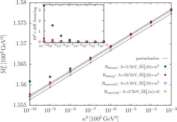
Figure 1: Longitudinal squared gap mass at the lowest available momentum as a function of the IR regulator parameter. The perturbative dependence (13) is also shown, with $\kappa_{0}$ fitted. Three different values of $\kappa_{0}$ are needed for the four sets of points, since only the leading behavior is regulator-independent. The deviation from the logarithmic behavior of the points obtained with a sharp UV regulator is caused by the non-analyticity of the regulator. The inset shows the difference of each point set to the corresponding perturbative (logarithmic) behavior.

3.2.1 Physical parameters

In Fig. 1 we compare $\bar{M}_{\mathrm{L}}^{2}$ at the lowest available momentum bin in different UV and IR regularizations. Concerning the numerical implementation of the constraint $\bar{M}^{2}_{\mathrm{T}}(0)=0$, in the case of the green squares, red blobs and blue circles we use the IR regularization (14), whereas for the yellow triangles we use (15). All four sets of points are compared to the corresponding perturbative result which displays a logarithmic dependence with respect to the IR regulator. This comparison reveals the following. The results obtained using a sharp UV regularization deviate at some point from the logarithm and, in the case of the smaller cutoff, they seem to reach a plateau, suggesting that an IR limit exists, as anticipated above. However, increasing the value of the cutoff makes the deviation to occur at smaller $\kappa$, which shows that the effect of the anomalous behavior is reduced as the cutoff is increased and suggests that above some value of the cutoff, the behavior of the solution as $\kappa$ is decreased should be essentially the same as that with a smooth UV regulator. In this latter case, the results follow the perturbative logarithmic behavior down to values of $\kappa$, where we reach the limits of our numerical precision. This can be seen also in the inset of Fig. 1 where the difference to the perturbative result is shown.

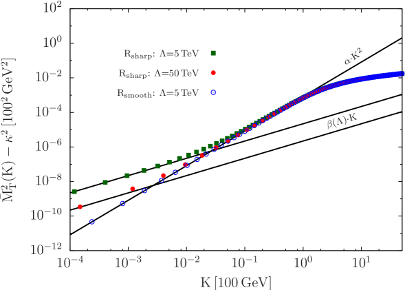
Figure 2: Deep IR behavior of the transverse self-energy. As the ultraviolet cutoff is increased, the importance of the anomalous, non-quadratic behavior in the case of a sharp UV regulator is reduced and the results approach those obtained with the smooth UV regulator. The coefficient $\beta(\Lambda)$ is the perturbative one which follows from (12) with $M^{2}\to\bar{M}^{2}_{\mathrm{L}}(0)$ while $\alpha=8.27\cdot 10^{-4}$ is obtained through fitting.

The different behavior displayed by $\bar{M}_{\mathrm{L}}^{2}$, depending on the chosen UV regulator, can be understood from the IR momentum behavior of $\bar{M}_{\mathrm{T}}^{2}(K)$, in line with the discussion of the previous section. This is shown in Fig. 2, where one can see that in the case of a sharp UV regulator, a linear term is present in the transverse squared gap mass at small $K$, with a prefactor which follows exactly from (12). In contrast, with a smooth UV regulator the transverse self-energy depends quadratically on the momentum in the deep IR and therefore according to the argument of Sec. 2.2 we expect a loss of solution in this case. Unfortunately, for the parameters used in Figs. 1 and 2 (set A of Table 1) the numerical check of the loss of solution turned out to be beyond reach, as we are limited by numerical precision. To visualize the loss of solution, we now switch to better suited sets of parameters.

3.2.2 Illustrative parameters

Using the parameter sets B and C given in Table 1, we now show that, at $T=0$, there are two different ways in which the physical solution is lost. We define $\kappa_{\varnothing}$ as the value of the IR regulator parameter at which the solution is lost. By losing the solution we mean that, for $\kappa<\kappa_{\varnothing}$, the coupled gap equations together with the constraint which determines the field expectation value have no solution which satisfies $\bar{\phi}^{2}>0$ and that can be reached by our iterative method. Of course, there could be solutions not reachable by the iterative method, but we believe that this is not the case for the physical solution. For the parameter set B, the loss of the physical solution happens due to the logarithmic IR sensitivity of the transverse bubble, while for the parameter set C, $\bar{\phi}^{2}$ becomes negative at $\kappa_{\varnothing}$.

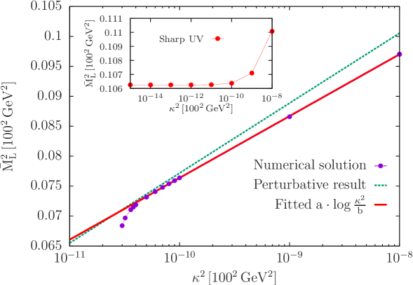
Figure 3: Loss of solution with decreasing $\kappa$ using parameter set B. The points are obtained with the IR regularization scheme (14), using $N_{\mathrm{S,cub}}=501$ and the smooth UV regulator (10) with $\Lambda=5~{}\mbox{TeV}$. The dashed green line is the perturbative expression (13), while the red line is the result of a fit. (For interpretation of the references to color in this figure legend, the reader is referred to the web version of this article.)

First we discuss the results obtained using parameter set B. In this case, the coupling was increased compared to set A in an attempt to enhance the logarithmic sensitivity as much as possible, while keeping the scale of the Landau pole far enough from the physical scales, see Table 1. We expected that at large coupling it would be easier to capture numerically the effect of the IR sensitivity than it was the case for the parameter set A. As shown in Fig. 3, the solution in the case of a smooth UV regulator is indeed lost below some $\kappa_{\varnothing}$. The logarithmic behavior of $\bar{M}^{2}_{\rm L}$ as a function of $\kappa^{2}$ abruptly changes, just above $\kappa_{\varnothing}$. This points in the direction that the loss of solution at small $\kappa$ is indeed caused by the logarithmic IR sensitivity, which in the end ruins the solution of the equation. Similar features have been observed in the conventional $\Phi$-derivable expansion scheme, when trying to approach a critical point [13]. Notice that the coefficient multiplying the logarithm changes, compared to the perturbative one. We believe that this is due to the non-perturbative corrections the self-energies receive. In the case of a sharp regulator, with $\Lambda=5~{}\mbox{TeV}$, it seems that we have a solution down to $\kappa=0$, as shown in the inset of Fig. 3. However, the proximity of the Landau pole ($\Lambda_{\mathrm{p}}/\Lambda\sim 10$) does not allow us to test whether this solution disappears for large enough $\Lambda$. In order to test this scenario, one should choose parameters (smaller values of $\lambda$) such that $\Lambda_{\mathrm{p}}$ is much further away from the physical scales. In such cases, the scale $\kappa_{\varnothing}$ becomes smaller and smaller, and it is difficult to see the loss of solution numerically. But as already explained in Sec. 2.2.2, in any case, the sharp UV regulator leads to inconsistent results.

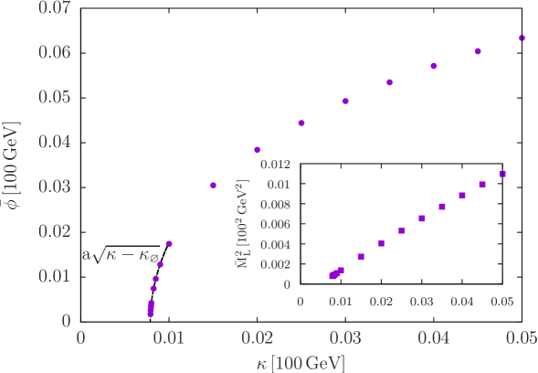
Figure 4: Loss of solution with decreasing $\kappa$ using parameter set C. More details on the mechanism are given in the text.

Turning now to the results obtained with the parameter set C, we show in Fig. 4 the field expectation value as a function of $\kappa$. Close to $\kappa_{\varnothing}$, $\bar{\phi}(\kappa)\sim\sqrt{\kappa-\kappa_{\varnothing}}$ is a good estimate, as indicated by the fit, which also suggests the disappearance of the solution. The inset shows that $\bar{M}_{\mathrm{L}}^{2}$, although decreasing linearly, is still non-vanishing at $\kappa_{\varnothing}$. The simple reason why this happens is that for the parameters of set C no broken phase exists. The criterion for a broken phase to exist at zero temperature (forgetting about IR problems for a moment) is that $T_{c}>0$, of course. Since at the critical temperature $\bar{\phi}=\bar{M}_{\mathrm{L}}=\bar{M}_{\mathrm{T}}=0$, a very simple equation determines the line in the parameter space where the system is critical at zero temperature. This equation is obtained using the gap equations at $\phi=0$ with vanishing masses. It is found using a sharp regulator that

$$-m^{2}=\frac{\lambda}{3}{\mathcal{T}}_{F}[G_{0}]=\frac{\lambda}{48\pi^{2}}\frac{\Lambda^{2}\mu^{2}}{\Lambda^{2}+\mu^{2}}\equiv-m_{\mathrm{c}}^{2}(\lambda).$$ (21)

The result obtained with a smooth regulator with cutoff $\Lambda$ is practically the same, however it is only available numerically.

For $m^{2}<m^{2}_{\mathrm{c}}(\lambda)$ the critical temperature is larger than zero, thus it is meaningful to search for a $\bar{\phi}^{2}>0$ solution, on the other hand, if $m^{2}>m^{2}_{\mathrm{c}}(\lambda)$, there is only the symmetric phase solution ($\bar{\phi}=0$) at $T=0$ with $\bar{M}_{\mathrm{L}}=\bar{M}_{\mathrm{T}}>0$. Plugging the parameters of set C into the expression of $m^{2}_{\mathrm{c}}(\lambda)$ we see that, indeed, only a symmetric phase could exist at sufficiently large $\Lambda$.

4 Loss of solution at finite temperature

In this section we investigate the loss of solution at finite temperature, numerically. We choose a representative temperature value $T=30~{}\mbox{GeV}$ and, using the parameter set A, we monitor the solution as a function of $\kappa$. Due to the employed numerical method, which is based on Fast Fourier Transform (FFT) (for more details, see A), we must use a combination of the IR regularization schemes of (14) and (15), that is

$$\bar{M}^{2}_{\rm T}\left(\omega_{n}=0,\frac{\Lambda}{N_{s}}\right)=\kappa^{2},$$ (22)

where, because the Fourier grid should resolve the smallest available scale $\kappa$, we should require that the ratio $c=\kappa N_{s}/\Lambda$ of this scale to the lattice spacing $\Delta k=\Lambda/N_{s}$ be ideally much greater than $1$. We use a finite number $N_{\tau}$ of Matsubara modes and we check that the dependence of our results on $N_{\tau}$ is negligible. Also, in contrast to the $T=0$ case, we apply a 3d UV regulator $R(q/\Lambda)$. In the case of the sharp regulator, the bubble of (18a) reads

$${\mathcal{B}}_{T=0}[G_{\mu}]=\frac{1}{8\pi^{2}}\left(\ln\frac{\Lambda+\varepsilon_{\Lambda}}{\mu}-\frac{\Lambda}{\varepsilon_{\Lambda}}\right)\,,$$ (23)

with $\varepsilon_{\Lambda}=\sqrt{\Lambda^{2}+\mu^{2}}$. We also have to adjust the calculation of the finite tadpole (19b) in the following way. To enhance the $N_{\tau}$ convergence we compute the difference of tadpoles as

$${\mathcal{T}}[\bar{G}_{\text{L/T}}]-\mathcal{T}_{T=0}[G_{\mu}] = \int_{Q}^{T}\big{[}\bar{G}_{\text{L/T}}(Q)-G_{\mu}(Q)\big{]}+\frac{1}{2\pi^{2}}\int_{0}^{\Lambda}dq\,q^{2}\frac{n_{\varepsilon_{q}}}{\varepsilon_{q}},$$ (24)

where $\varepsilon_{q}=\sqrt{q^{2}+\mu^{2}}$ and $n_{x}=1/(\exp(x/T)-1)$ is the Bose–Einstein statistical factor. For the second line of (18b) we use the relation

$$\int_{Q}^{T=0}G_{\mu}^{2}(Q)\,\Big{[}{\mathcal{B}}_{T=0}[G_{\mu}](Q)-{\mathcal{B}}_{T=0}[G_{\mu}]\Big{]}\equiv-\left[\frac{1}{3}\frac{\partial{\mathcal{S}}_{T=0}[G_{\mu}]}{\partial\mu^{2}}+({\mathcal{B}}_{T=0}[G_{\mu}])^{2}\right],$$ (25)

with $\mathcal{S}_{T=0}[G_{\mu}]$ taken from equation (B20) of [17], where it was calculated with a 3d cutoff.

We mention that the calculation of the perturbative bubble done in C with a 3d sharp UV regulator reveals, in its vacuum part, a linear dependence with respect to small external momenta (see (42)), similar to the one obtained with a 4d regulator. The thermal part also displays such a dependence but with a prefactor which is suppressed by a factor of $\exp(-\Lambda/T)$. As in the $\smash{T=0}$ case, this has to be considered an artifact and from now on we switch to a smooth UV regulator. In this case, we replace the expression in (23) and (24) with integrals calculated using $R_{\text{smooth}}(q/\Lambda)$.

In the limit $c\to\infty$ (and $\kappa$ kept small) the IR regularization (22) results in $\bar{M}^{2}_{\rm L}$ being dominated by the non-perturbative bubble ${\mathcal{B}}[\bar{G}_{\mathrm{T}}]$ at zero-momentum, with $\bar{M}^{2}_{\rm T}(0,0)=\kappa^{2}$. Thus, using the high temperature expansion in a perturbative zero-momentum bubble with mass $\kappa$ gives us the perturbative estimate of the dependence of $\bar{M}^{2}_{\rm L}$ for small $\kappa$ (before the loss of solution):

$$\sim\frac{\lambda^{2}}{576\pi}\phi^{2}\frac{T}{\kappa}+\mathit{const.}\ ,$$ (26)

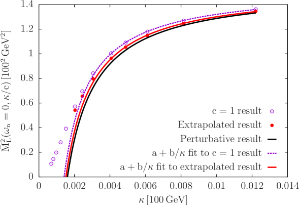
Figure 5: Loss of solution with decreasing $\kappa$ using the parameter set A at a temperature $T=30~{}\mbox{GeV}$. Notice that $\bar{M}^{2}_{\rm L}$ does not become zero. The perturbative result is given in (26). The red blobs come from extrapolating to $c=\infty$ results obtained at finite $c$. (For interpretation of the references to color in this figure legend, the reader is referred to the web version of this article.)

which foretells a faster loss of solution than in the zero temperature case due to the stronger (linear) sensitivity of the transverse bubble diagram. Indeed, as shown in Fig. 5 the solution is lost at some $\kappa_{\varnothing}$, where still $\bar{M}^{2}_{\rm L}\neq 0$. In practice this means that we found no iterative solution with the lowest value $\alpha=10^{-3}$ used in the under-relaxation method (see Eq. (135) of [17]). It also can be seen that when $a+b/\kappa$ is fitted to the data, the extrapolation to $c=\infty$ of results obtained at $c\in\{1,2,4,8\}$ pushes the coefficient of $\kappa^{-1}$ of the fit closer to its perturbative value. Furthermore, we see that the qualitative behavior of the solution changes before the solution is truly lost. This is probably due to the inherent inaccuracy of the discrete sine transform for light modes with small momenta.

Figure 6: The deep IR behavior of $\bar{M}^{2}_{\rm T}$ at the leftmost red blob of Fig. 5, where $\kappa\approx 0.002\times 100~{}\mbox{GeV}$. Notice that the y-axis is scaled by $k^{2}$.

Another evidence that suggests that an infinite volume limit cannot be reached is the IR behavior of the self-energy $\bar{M}^{2}_{\rm T}(\omega_{n}=0,k)$, which we show in Fig. 6. There, we see that the momentum dependence in the deep IR gradually conforms to $\sim k^{2}$, as $c$ is increased. As far as this behavior persists, according to our argument in Sec. 2.2, a loss of solution is to be expected at small enough $\kappa$. This was observed already in [13] (see Fig. 16 there) with a cruder IR regularization. There, instead of the regularization (22), we used $\bar{M}^{2}_{\mathrm{T}}(\omega_{n}=0,\Delta k)=0$, which enhances the error of the discrete sine transform, as the lowest momentum mode becomes massless.

5 Conclusions

We studied the implications of the symmetry improved approach, recently proposed in [9], on the solution of the $O(2)$-symmetric scalar model, by using a truncation at two-loop level of the 2PI effective action.

We argued that, due to an untamed IR sensitivity at this approximation order, the constraint imposed in this approach on the transverse gap mass ($\bar{M}_{\mathrm{T}}(K=0)=0$) leads to a loss of the solution to the set of coupled gap equations, unless an anomalous dimension is generated. This seems not to be the case for smooth enough UV regulators, where our numerical study, both at zero and finite temperature, supports our claim that the solution is lost. We tried various numerical implementations of the above constraint, all involving an IR regulating parameter $\kappa$, and showed that when one tries to reach the $\kappa\to 0$ limit, the iterative solution is lost at some finite $\kappa$. At zero temperature, the way this loss of solution happens in different regions of the parameter space lead us to believe that this is a general feature of the symmetry improved approach at the present level of truncation. It has to do with the numerically observed logarithmic IR sensitivity and is not related to the iterative method used. At finite temperature, the IR sensitivity is stronger (linear), however, our FFT based numerical method makes accurate investigations more difficult. In this case, although the loss of solution is quite convincing and in line with the preliminary finding of our previous study [13], we cannot exclude in principle the possibility that the absence of solution is due to the fact that the iterative method cannot converge, hence further investigation with a different numerical method is required. For certain non-analytic UV regulators, an anomalous dimension is present which, if strong enough, can lead to an infinite volume solution for a fixed value of the UV cutoff. We argued that this solution should be considered as an artifact in any situation where the dependence to the UV regulator can be removed or considerably reduced by taking large enough values of $\Lambda$ (although it could be relevant in situations where such a UV cutoff has a physical origin).

We mention that there can be parameters, to which physical parameters may or may not belong, at which a loss of solution can be observed numerically only if an extremely fine resolution can be achieved in the deep IR. In those cases our present investigation should be regarded as a warning: when a self-consistent propagator equation obtained in a given truncation is unable to generate an anomalous dimension, then IR divergences could remain untamed. Therefore, it would be interesting to test the features of the symmetry improved approach at higher level truncation of the 2PI effective action, in particular in the next-to-leading order of the 2PI-$1/N$ expansion, where an anomalous dimension is known to be generated at the critical point.

Another possible way to circumvent the difficulty is to recognize that the infinite volume limit is just a convenient mathematical limit (when it can be taken) but, in principle, any physical system has a finite size. It may then be that, in some cases of interest, the loss of solution occurs at a value of $\kappa_{\varnothing}$ way below the inverse linear size $\pi/L$ of the system. For instance, and without trying to be rigorous, in the case of the application to Higgs physics of [9], a rough estimate of the maximal linear size obtained from $\kappa_{\varnothing}$ using a simplification (localization as in [13]) of the equations is still more than 200 orders of magnitude larger than the size of the observable Universe. Keeping in mind that by doing such estimates one might overpass the validity of this field theoretical model, one can reverse this argument, which then tells us that using the parameters of [9] and taking $\kappa$ to be inversely proportional to the scale of the observable Universe would result in a $\approx 5\%$ underestimation of the Higgs mass.

Appendix A Numerics

In this Appendix, the interested reader may find more details on the numerical procedure we carried out. We concentrate on the $T=0$ case. For the finite temperature analysis we direct the reader to the original paper [17] where various techniques that we employ here have been introduced and described in detail. However we point out that we use fast Fourier transform to compute convolutions, which restricts our choice of discretization to a uniform grid, with a non-zero first momentum bin. It also needs to be mentioned that the convergence of the Fourier transform is only ensured for massive propagators. These two features dictate our choice of IR regularization scheme (22).

We either solved the coupled gap equations at fixed $\phi$ (that is (16a) and (16b)) or together with (20), which comes from the constraint $\bar{M}^{2}_{\mathrm{T}}(0)=0$. Both systems of equations contain a self-consistent self-energy function to be solved for, which we approximate using iterations. We discretize the self-energy over a certain set of $N_{\mathrm{S}}$ momentum values, use spline interpolation to have its value for other momenta and compute all integrals using the GNU Scientific Library [20], similarly as in [9]. However, we use two different discretizations. A uniform one, where

$$K_{i}=K_{\mathrm{min}}+i\frac{K_{\mathrm{max}}-K_{\mathrm{min}}}{N_{\mathrm{S}}-1},$$ (27)

and a cubic, non-equidistant one which has resolution concentrated in the IR region. There

$$K_{i}=K_{\mathrm{min}}+i^{3}\frac{K_{\mathrm{max}}-K_{\mathrm{min}}}{(N_{\mathrm{S}}-1)^{3}},$$ (28)

with $i=0,\dots,N_{\mathrm{S-1}}$ in both cases. $K_{\mathrm{min}}$ and $K_{\mathrm{max}}$ are, respectively, the smallest and largest available momentum on the grid. In case of the IR regularization (14) $K_{\mathrm{min}}=0$, while for the IR regularization (15) $K_{\mathrm{min}}=\kappa$. The discretization itself affects certain aspects of the IR/UV regularization. First of all, due to the finite number of available points, even the use of the smooth UV regulator (10) requires the use of a sharp cutoff. The smooth regulator function $R_{\text{smooth}}(K/\Lambda)$ of the form (10) has as a function of the momentum $K$ an inflection at the value of the physical cutoff $\Lambda$ used, that is at $K=\Lambda$. The value $\sigma=50$ guaranties a sharp variation of the regulator function around the inflection point and a fast diminishing of its value as the momentum is increased. We use $K_{\mathrm{max}}\approx 1.5-2\ \Lambda$, for which the value of the regulator function is approximately $10^{-13}$. The second implication of the discretization on the regularization only appears in case of the IR regularization scheme (15). In this case the momentum discretization starts at $\kappa$, and therefore any lower boundary of integration has to be bounded from below by $\kappa$. In this sense the discussed IR regularization scheme is twofold, as no integral has zero as a lower boundary.

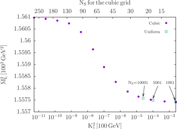
Figure 7: Discretization dependence of the IR regularized $\bar{M}_{\mathrm{L}}^{2}(K=0)$, where $K_{1}$ is defined as the lowest non-zero momentum bin in both cubic and uniform grids. We used a sharp UV regulator with cutoff $\Lambda=5~{}\mbox{TeV}$ and the IR regularization scheme $\bar{M}_{\mathrm{T}}^{2}(0)=\kappa^{2}$ with $\kappa=10^{-5}\times 100~{}\mbox{GeV}$.

The introduction of the cubic grid proves to be very useful, because high IR resolution can be achieved with a uniform grid only for huge $N_{\mathrm{S}}$ values. This is illustrated in Fig. 7, where one can see that in comparison to the uniform grid, the cubic grid needs only a few points and therefore makes computations more economic.

Appendix B Counterterms

We describe bellow how to derive with the method summarized in Sec. 3.1 the explicit relation between bare and renormalized parameters, that is how to obtain the expression of the counterterms.

First, we subtract the finite gap equations from the bare ones, using for the tadpole and bubble integrals the decomposition into finite and divergent pieces. The latter are given in (18) and we use for the local gap mass squared $\bar{M}^{2}_{\text{L/T,l}}$ their explicit expression which can be read off from (16). We end up with two equations, one coming from the transverse sector and one from the longitudinal one, in which the finite quantities $\phi^{2}$ and $\mathcal{T}_{\text{F}}[\bar{G}_{\text{L/T}}]$ are multiplied by a combination of bare couplings and divergent integrals. The bare couplings (or counterterms) are obtained by requiring the vanishing of the coefficients of the above finite quantities, while the remnant gives the unique relation

$$m_{0}^{2}=m^{2}-\frac{\lambda_{0}^{(A+B)}}{6}\big{[}{\mathcal{T}}_{T=0}[G_{\mu}]+(\mu^{2}-m^{2}){\mathcal{B}}_{T=0}[G_{\mu}]\big{]}\,.$$ (29)

From the vanishing of the coefficients of $\mathcal{T}_{\text{F}}[\bar{G}_{\text{L}}]$ and $\mathcal{T}_{\text{F}}[\bar{G}_{\text{T}}]$ we obtain the relations

$$\frac{1}{\lambda_{0}^{(A+B)}}=\frac{1}{2\lambda}-\frac{{\mathcal{B}}_{T=0}[G_{\mu}]}{6},\quad\frac{1}{\lambda_{0}^{(B)}}=\frac{1}{\lambda}-\frac{{\mathcal{B}}_{T=0}[G_{\mu}]}{6}.$$ (30)

The vanishing of the coefficient of $\phi^{2}$ in the two equations determines $\lambda_{2}^{(A/B)}=\lambda+\delta\lambda_{2}^{(A/B)}$. We split the counterterms into a local and a nonlocal part and write $\lambda_{2}^{(A/B)}=\lambda_{\text{2,l}}^{(A/B)}+\delta\lambda_{\text{2,nl}}^{(A/B)}$, where the nonlocal part given by $\delta\lambda_{\text{2,nl}}^{(B)}=2\delta\lambda_{\text{2,nl}}^{(A)}=\frac{2\lambda^{2}}{3}{\mathcal{B}}_{T=0}[G_{\mu}]$ is used to remove the divergence of the bubble integral in the self-energy. The two conditions determining the local part of the counterterms can be written in a compact form using the pairs $\alpha=A+2B$, $\beta=A$ and $\alpha=A$, $\beta=A+2B$ as follows:

$$\delta\lambda_{\text{2,l}}^{(\alpha)} = \frac{\lambda\lambda_{0}^{(\alpha)}}{4}\left[{\mathcal{B}}_{T=0}[G_{\mu}]-\frac{5\lambda}{9}{\mathcal{T}}_{\mathrm{d}}^{({\mathcal{B}})}\right]+\frac{\lambda\lambda_{0}^{(\beta)}}{12}\left[{\mathcal{B}}_{T=0}[G_{\mu}]-\frac{\lambda}{3}{\mathcal{T}}_{\mathrm{d}}^{({\mathcal{B}})}\right],$$ (31)

with

$${\mathcal{T}}_{\mathrm{d}}^{({\mathcal{B}})}\equiv\int_{Q}^{T=0}G_{\mu}^{2}(Q)\,\Big{[}{\mathcal{B}}_{T=0}[G_{\mu}](Q)-{\mathcal{B}}_{T=0}[G_{\mu}]\Big{]}\,.$$ (32)

Note that the expressions (29), (30), and (31) are identical in form with those coming in [15] from renormalization prescriptions imposed at temperature $T_{\star}$.

Now, as a last step, one can check that, by using the relations between bare and finite parameters, the finite gap equations are obtained from the bare ones. For this one first uses (29) and (31) in the bare gap equations. Then, one constructs two combinations $\bar{M}^{2}_{\text{L}}(K)-\bar{M}^{2}_{\text{T}}(K)$ and $\bar{M}^{2}_{\text{L}}(K)+\bar{M}^{2}_{\text{T}}(K)$ and applies (30). After recognizing in these equations the appearance of the finite tadpoles given in (19b), one just turns back from the equations for the two linear combinations to those for $\bar{M}^{2}_{\text{L}}$ and $\bar{M}^{2}_{\text{T}}$, to obtain (16).

Appendix C Perturbative bubble with a sharp regulator

In this section and for the sake of clarity, $K$ denotes the norm of $K$ when this is obvious. The perturbative bubble with a sharp 4d regulator at the level of the propagators has been computed in [19]. In the case where one of the propagators is massless, we obtain

$${\mathcal{B}}_{\mathrm{pert}}[G,G_{0}](K) =\frac{1}{4\pi^{3}}\int_{0}^{\Lambda}dQ\,\frac{Q^{3}T(Q,K,0,-1)}{Q^{2}+M^{2}}$$

$$+\frac{1}{4\pi^{3}}\int_{\Lambda-K}^{\Lambda}dQ\,\frac{Q^{3}\Delta T(Q,K,0,\alpha)}{Q^{2}+M^{2}}\,,\qquad$$ (33)

where

$$T(Q,K,0,\alpha) =\,\frac{1}{4Q^{2}K^{2}}\left[\vphantom{\sqrt{\frac{1-\alpha}{1+\alpha}}}2Q\,K\sqrt{1-\alpha^{2}}+\big{(}Q^{2}+K^{2}\big{)}\arccos\,\alpha\right.$$

$$\left.-\,2|Q^{2}-K^{2}|\arctan\,\left(\frac{Q+K}{|Q-K|}\sqrt{\frac{1-\alpha}{1+\alpha}}\right)\right],$$ (34)

and $\smash{\Delta T(Q,K,0,\alpha)=T(Q,K,0,\alpha)-T(Q,K,0,-1)}$, with $\alpha\equiv(K^{2}+Q^{2}-\Lambda^{2})/(2KQ)$. In particular

$$T(Q,K,0,-1) = \frac{\pi}{2}\frac{1}{\mathrm{Max}(Q^{2},K^{2})}\,.$$ (35)

To study the small $K$ behavior, we note that, as $K\to 0$, we can always assume that $K<\Lambda$ and thus the first contribution to (C) reads

$$\frac{1}{8\pi^{2}K^{2}}\int_{0}^{K}dQ\,\frac{Q^{3}}{Q^{2}+M^{2}}+\frac{1}{8\pi^{2}}\int_{K}^{\Lambda}dQ\,\frac{Q}{Q^{2}+M^{2}}\,.$$ (36)

The integrals can be easily done and the expansion of the result does not contain any linear term in $K$ at small $K$.

In the second contribution to (C), since $Q>\Lambda-K$, we can always assume that $Q>K$ in the limit $K\to 0$. We rescale the integration variable by $K$ and shift the new integration variable by $x=\Lambda/K$. Denoting the integrand by $h(Q,K,L)$, this yields

$$\frac{1}{4\pi^{3}}\int_{\Lambda-K}^{\Lambda}dQ\,h(Q,K,\Lambda)=\frac{1}{4\pi^{3}}\int_{-1}^{0}d\bar{Q}\,h(\bar{Q}+x,1,x).$$

We can now expand the integrand for $x\to\infty$ and we obtain

$$\sim\frac{1}{8\pi^{3}}\frac{x^{-1}}{1+\frac{M^{2}}{\Lambda^{2}}}\int_{-1}^{0}d\bar{Q}\,\left\{\arccos\,\bar{Q}-\bar{Q}\sqrt{1-\bar{Q}^{2}}-\pi\right\}.$$ (37)

Computing this last integral, we finally arrive at

$${\mathcal{B}}_{\mathrm{pert}}[G,G_{0}](K)-{\mathcal{B}}_{\mathrm{pert}}[G,G_{0}]\sim-\frac{1}{12\pi^{3}}\frac{K\Lambda}{\Lambda^{2}+M^{2}}\,.$$ (38)

In contrast, applying the same considerations to the perturbative bubble with a sharp regulator applied at the level of the loop, and not at the level of the propagators, we do not obtain a linear $K$ behavior at small $K$. Similarly there is no linear behavior in the presence of a smooth regulator.

At finite temperature, the same bubble with a $3$d sharp propagator regulator reads

$${\mathcal{B}}_{\mathrm{pert}}[G,G_{0}](K)= \,\frac{1}{8\pi^{2}k}\int_{0}^{\Lambda}dq\,q\Bigg{[}\frac{1+2n_{\varepsilon_{q}}}{2\varepsilon_{q}}{\mathrm{Re}}\,\ln\frac{-(\varepsilon_{q}-i\omega)^{2}+(k+q)^{2}}{-(\varepsilon_{q}-i\omega)^{2}+(k-q)^{2}}$$

$${}+\frac{1+2n_{q}}{2q}{\mathrm{Re}}\,\ln\frac{-(q-i\omega)^{2}+\varepsilon_{k+q}^{2}}{-(q-i\omega)^{2}+\varepsilon_{k-q}^{2}}\Bigg{]}$$

$${}+\frac{1}{8\pi^{2}k}\int_{\Lambda-k}^{\Lambda}dq\,q\Bigg{[}\frac{1+2n_{\varepsilon_{q}}}{2\varepsilon_{q}}{\mathrm{Re}}\,\ln\frac{-(\varepsilon_{q}-i\omega)^{2}+\Lambda^{2}}{-(\varepsilon_{q}-i\omega)^{2}+(k+q)^{2}}$$

$${}+\frac{1+2n_{q}}{2q}{\mathrm{Re}}\,\ln\frac{-(q-i\omega)^{2}+\varepsilon_{\Lambda}^{2}}{-(q-i\omega)^{2}+\varepsilon_{k+q}^{2}}\Bigg{]}\,.$$ (39)

The contributions involving the integrals from $0$ to $\Lambda$ are of order $k^{2}$ as $k\to 0$, as is easily checked by expanding the integrands. The contributions involving the integrals from $\Lambda-k$ to $\Lambda$ are treated using the change of variables $q=kx+\Lambda$ and expanding the integrand at small $k$. For instance

$$\frac{1}{8\pi^{2}}\int_{-1}^{0}dx\,\left(kx+\Lambda\right)\frac{1+2n_{\varepsilon_{kx+\Lambda}}}{2\varepsilon_{kx+\Lambda}}\mathrm{Re}\,\ln\frac{-(\varepsilon_{kx+\Lambda}-i\omega)^{2}+\Lambda^{2}}{-(\varepsilon_{kx+\Lambda}-i\omega)^{2}+(k+kx+\Lambda)^{2}}$$

$$\quad\sim\frac{k}{8\pi^{2}}\frac{1+2n_{\varepsilon_{\Lambda}}}{\varepsilon_{\Lambda}}\frac{\Lambda^{2}(m^{2}-\omega^{2})}{(m^{2}-\omega^{2})^{2}+4\omega^{2}(\Lambda^{2}+m^{2})}\underbrace{\int_{-1}^{0}dx\,(1+x)}_{1/2}\,.$$ (40)

Together with a similar contribution from the other integral, we obtain

$$\sim\frac{k}{8\pi^{2}}\Bigg{[}\frac{1+2n_{\varepsilon_{\Lambda}}}{2\varepsilon_{\Lambda}}\frac{\Lambda^{2}(m^{2}-\omega^{2})}{(m^{2}-\omega^{2})^{2}+4\omega^{2}(\Lambda^{2}+m^{2})}-\frac{1+2n_{\Lambda}}{2\Lambda}\frac{\Lambda^{2}(m^{2}+\omega^{2})}{(m^{2}+\omega^{2})^{2}+4\omega^{2}\Lambda^{2}}\Bigg{]}\,.$$ (41)

We thus find a linear $k$-dependence at small $k$. Its finite temperature contribution is suppressed by a factor $e^{-\Lambda/T}$. The zero temperature contribution is suppressed by a factor $1/\Lambda$. This is obvious for $\omega\neq 0$. For $\omega=0$, one needs to combine the two contributions

$$\sim\frac{k}{16\pi^{2}}\frac{\Lambda^{2}}{m^{2}}\left[\frac{1}{\varepsilon_{\Lambda}}-\frac{1}{\Lambda}\right]\sim-\frac{1}{32\pi^{2}}\frac{k}{\Lambda}\,.$$ (42)

References

- [1] J. Berges, “Nonequilibrium Quantum Fields: From Cold Atoms to Cosmology,” arXiv:1503.02907 [hep-ph].
- [2] G. Baym and G. Grinstein, Phys. Rev. D 15, 2897 (1977).
- [3] J. P. Blaizot, E. Iancu and A. Rebhan, Phys. Rev. D 63, 065003 (2001).
- [4] J. Berges, Sz. Borsányi, U. Reinosa and J. Serreau, Phys. Rev. D 71, 105004 (2005).
- [5] J. P. Blaizot, A. Ipp, A. Rebhan and U. Reinosa, Phys. Rev. D 72, 125005 (2005).
- [6] Y. B. Ivanov, F. Riek, H. van Hees and J. Knoll, Phys. Rev. D 72, 036008 (2005).
- [7] V. I. Yukalov and H. Kleinert, Phys. Rev. A 73, 063612 (2006).
- [8] S. Leupold, Phys. Lett. B 646, 155 (2007).
- [9] A. Pilaftsis and D. Teresi, Nucl. Phys. B874, 594 (2013).
- [10] M. J. Brown and I. B. Whittingham, Phys. Rev. D 91, no. 8, 085020 (2015)
- [11] B. Garbrecht and P. Millington, Nucl. Phys. B906, 105 (2016).
- [12] A. Pilaftsis and D. Teresi, Nucl. Phys. B906, 381 (2016).
- [13] G. Markó, U. Reinosa and Zs. Szép, Phys. Rev. D 92, 125035 (2015).
- [14] M. J. Brown, I. B. Whittingham and D. S. Kosov, Phys. Rev. D 93, 105018 (2016).
- [15] G. Markó, U. Reinosa and Zs. Szép, Phys. Rev. D 87, 105001 (2013).
- [16] J. Berges, S. Borsányi, U. Reinosa and J. Serreau, Ann. Phys. (N.Y) 320, 344 (2005).
- [17] G. Markó, U. Reinosa and Zs. Szép, Phys. Rev. D 86, 085031 (2012).
- [18] A. Patkós and Zs. Szép, Nucl. Phys. A811, 329 (2008).
- [19] U. Reinosa and Zs. Szép, Phys. Rev. D 85, 045034 (2012).
- [20] M. Galasi et al., GSL Reference Manual (Version GSL-2.1, 2015), http://www.gnu.org/software/gsl .