A Generalized Fundamental Matrix for Computing Fundamental Quantities of Markov Systems

Abstract

As is well known, the fundamental matrix $(\bm{I}-\bm{P}+\bm{e}\bm{\pi})^{-1}$ plays an important role in the performance analysis of Markov systems, where $\bm{P}$ is the transition probability matrix, $\bm{e}$ is the column vector of ones, and $\bm{\pi}$ is the row vector of the steady state distribution. It is used to compute the performance potential (relative value function) of Markov decision processes under the average criterion, such as $\bm{g}=(\bm{I}-\bm{P}+\bm{e}\bm{\pi})^{-1}\bm{f}$ where $\bm{g}$ is the column vector of performance potentials and $\bm{f}$ is the column vector of reward functions. However, we need to pre-compute $\bm{\pi}$ before we can compute $(\bm{I}-\bm{P}+\bm{e}\bm{\pi})^{-1}$. In this paper, we derive a generalization version of the fundamental matrix as $(\bm{I}-\bm{P}+\bm{e}\bm{r})^{-1}$, where $\bm{r}$ can be any given row vector satisfying $\bm{r}\bm{e}\neq 0$. With this generalized fundamental matrix, we can compute $\bm{g}=(\bm{I}-\bm{P}+\bm{e}\bm{r})^{-1}\bm{f}$. The steady state distribution is computed as $\bm{\pi}=\bm{r}(\bm{I}-\bm{P}+\bm{e}\bm{r})^{-1}$. The Q-factors at every state-action pair can also be computed in a similar way. These formulas may give some insights on further understanding how to efficiently compute or estimate the values of $\bm{g}$, $\bm{\pi}$, and Q-factors in Markov systems, which are fundamental quantities for the performance optimization of Markov systems.

Keywords: Fundamental matrix, performance potential, steady state distribution, Q-factors, stochastic matrix

1 Introduction

Markov decision processes (MDPs) are widely adopted to model the dynamic decision problem in stochastic systems [2, 14]. The fundamental matrix $(\bm{I}-\bm{P}+\bm{e}\bm{\pi})^{-1}$ plays a key role in the performance optimization of MDPs. With the fundamental matrix, we can further study the properties of Markov systems. For example, we can use it to compute the performance potential (or called relative value function) of MDPs under the average criterion, i.e., $\bm{g}=(\bm{I}-\bm{P}+\bm{e}\bm{\pi})^{-1}\bm{f}$.

The concept of the fundamental matrix was first proposed by J. G. Kemeny in his book “Finite Markov Chains” coauthored with L. J. Snell in 1960 [11]. In this book, the fundamental matrix is defined as $\bm{Z}^{*}:=(\bm{I}-\bm{P}+\bm{e}\bm{\pi})^{-1}$. Many analysis, such as the mean passage time and the variance of passage time, can be conducted by using this fundamental matrix. The fundamental matrix also plays a key role in the performance sensitivity analysis of Markov systems. The original work about the sensitivity analysis of the steady state distribution and the fundamental matrix with respect to the stochastic matrix of Markov systems can be referred backward to P. Schweitzer’s work in 1968 [15]. P. Schweitzer presented a perturbation formalism that shows how the stationary distribution and the fundamental matrix of a Markov chain containing a single irreducible set of states change as the transition probabilities vary. The sensitivity information can be represented in a series of Rayleigh perturbation expansions of the fundamental matrix and other parameters. This is the main target of the perturbation analysis of Markov chains at the early stage.

E. Seneta and C. D. Meyer did a lot of work [12, 17] to study the relation between the eigenvalues of stochastic matrix $\bm{P}$ and the condition number ($\max\{|a^{\#}_{i,j}|\}$) of group generalized inverse ($\bm{A}^{\#}=(\bm{I}-\bm{P}+\bm{e}\bm{\pi})^{-1}-\bm{e}\bm{\pi}$) of matrix $\bm{A}=\bm{I}-\bm{P}$, where $a^{\#}_{i,j}$ is the element of matrix $\bm{A}^{\#}$. Some inequalities are derived to quantify the sensitivity of the steady state distribution when $\bm{P}$ is perturbed to $\bm{P}^{\prime}$. Therefore, the sensitivity of the steady state distribution can be analyzed through studying the eigenvalues of stochastic matrix $\bm{P}$. This is the main idea of the perturbation analysis of Markov chains at that period. More than the sensitivity analysis of the steady state distribution, X. R. Cao proposed the sensitivity-based optimization theory that focuses on the sensitivity analysis of the system performance with respect to the perturbed transition probabilities or policies [3, 4]. This approach works well for different system settings, including the average or discounted criterion, the unichain or multichain, Markov or semi-Markov systems.

Performance potential $\bm{g}$ is a fundamental quantity in MDPs. We have to compute or estimate its value before we conduct the policy iteration or sensitivity-based optimization. For an MDP under the discounted criterion, we can directly compute it as $\bm{g}=(\bm{I}-\gamma\bm{P})^{-1}\bm{f}$ since the matrix $(\bm{I}-\gamma\bm{P})$ is invertible [14], where $\gamma$ is the discount factor and $0<\gamma<1$. For an MDP under the average criterion, the fundamental matrix is used to compute the value of performance potentials and it has the form $\bm{g}=(\bm{I}-\bm{P}+\bm{e}\bm{\pi})^{-1}\bm{f}$. Since the fundamental matrix can be decomposed as $(\bm{I}-\bm{P}+\bm{e}\bm{\pi})^{-1}=\sum_{n=0}^{\infty}(\bm{P}^{n}-\bm{e}\bm{\pi})$, we can rewrite the definition of the performance potential as $\bm{g}=\sum_{n=0}^{\infty}(\bm{P}^{n}\bm{f}-\eta\bm{e})$, where $\eta=\bm{\pi}\bm{f}$ is the long-run average performance. That is, we can derive the following sample path version of the performance potential as $g(i)=E\{\sum_{n=0}^{N}(f(X_{n})-\hat{\eta})|X_{0}=i\}$, where $X_{n}$ is the system state at time $n$, $\hat{\eta}$ is the estimated value of the long-run average performance, $i\in\mathcal{S}$ is a state of the state space $\mathcal{S}$, and $N$ is a proper integer that is to control the estimation variance [4]. However, we see that when we compute $\bm{g}=(\bm{I}-\bm{P}+\bm{e}\bm{\pi})^{-1}\bm{f}$, we have to pre-compute the value of $\bm{\pi}$ first. This issue was also pointed out by J. G. Kemeny when he studied the computation of the fundamental matrix $\bm{Z}^{*}=(\bm{I}-\bm{P}+\bm{e}\bm{\pi})^{-1}$. He wrote “It also suffers from the difficulty that one must compute $\alpha$ (solving $n$ equations) before one can compute $\bm{Z}^{*}$” [10], where $\alpha$ is the steady state distribution $\bm{\pi}$ in our paper.

In this paper, we study another form of the fundamental matrix as $\bm{Z}_{r}:=(\bm{I}-\bm{P}+\bm{e}\bm{r})^{-1}$, where $\bm{r}$ is any row vector satisfying $\bm{r}\bm{e}\neq 0$. Using this generalized fundamental matrix, we can compute the value of performance potentials as $\bm{g}=(\bm{I}-\bm{P}+\bm{e}\bm{r})^{-1}\bm{f}$, where all the parameters are known and no pre-computation is required. The traditional approach $\bm{g}=(\bm{I}-\bm{P}+\bm{e}\bm{\pi})^{-1}\bm{f}$ is a special case where we choose $\bm{r}=\bm{\pi}$. We can also choose $\bm{r}$ as other vectors. This formula can also be used to compute the value of $\bm{\pi}$ as $\bm{\pi}=\bm{r}(\bm{I}-\bm{P}+\bm{e}\bm{r})^{-1}$, where the kernel computation remains the same as the generalized fundamental matrix $(\bm{I}-\bm{P}+\bm{e}\bm{r})^{-1}$.

There exist two works about the generalization of the fundamental matrix in the literature. After proposing the concept of the fundamental matrix, J. G. Kemeny further studied a generalized form [10]. A special case for ergodic Markov chains is that he defined $\bm{Z}_{\beta}:=(\bm{I}-\bm{P}+\bm{e}\bm{\beta})^{-1}$, $\bm{\beta}\bm{e}=1$, where $\bm{\beta}$ is a row vector. In Kemeny’s work, it is shown that the above matrix can be used to compute the stationary distribution as $\bm{\pi}=\bm{\beta}\bm{Z}_{\beta}$. Similar result was later reported in J. J. Hunter’s book [7], which has the form $\bm{\pi}=\bm{u}(\bm{I}-\bm{P}+\bm{e}\bm{u})^{-1}$, $\bm{u}\bm{e}\neq 0$, where $\bm{u}$ is a row vector. After that, J. J. Hunter further gave a thorough study on varied forms of general inverse of Markovian kernel $(I-P)$ in his recent works [8, 9]. One form of the general inverse is written as $(\bm{I}-\bm{P}+\bm{t}\bm{u})^{-1}$ with condition $\bm{\pi}\bm{t}\neq 0$ and $\bm{u}\bm{e}\neq 0$, where $\bm{t}$ is a column vector. Obviously, $(\bm{I}-\bm{P}+\bm{t}\bm{u})^{-1}$ is more general than the above results. Although these works have a similar result to ours, they focus on the computation of the steady state distribution or the mean first passage time. There is no study on the computation of performance potentials or relative value functions. Compared with the widely-adopted form $\bm{g}=(\bm{I}-\bm{P}+\bm{e}\bm{\pi})^{-1}\bm{f}$, our new formula $\bm{g}=(\bm{I}-\bm{P}+\bm{e}\bm{r})^{-1}\bm{f}$ does not require the pre-computation of $\bm{\pi}$. It may shed some light on how to efficiently compute or estimate the value of $\bm{g}$, which is an essential procedure for the policy iteration in MDPs. Moreover, we also study the generalization of the fundamental matrix not only for a discrete time Markov chain, but also for a continuous time Markov process. We further extend the similar idea to the representation and computation of Q-factors that are fundamental quantities for reinforcement learning and artificial intelligence [18, 19].

2 Main Results

2.1 Generalized Fundamental Matrix

We focus on the discussion of a Markov chain with finite states. The state space is denoted as $\mathcal{S}:=\{1,2,\cdots,S\}$. The transition probability matrix is denoted as $\bm{P}$ and its element is $P(i,j)$ indicating the probability of which the system transits from the current state $i$ to the next state $j$, where $i,j\in\mathcal{S}$. The steady state distribution of this Markov chain is denoted as an $S$-dimensional row vector $\bm{\pi}$ and its element $\pi(i)$ is the probability of the system staying at state $i$, $i\in\mathcal{S}$. Obviously, we have

$$\bm{P}\bm{e}=\bm{e},\qquad\bm{\pi}\bm{P}=\bm{\pi},\qquad\bm{\pi}\bm{e}=1,$$ (1)

where $\bm{e}$ is an $S$-dimensional column vector with all elements 1.

First, we give the following lemma about shifting the eigenvalues of a general matrix.

Lemma 1.

Suppose that $\bm{A}$ is a square matrix for which $\lambda$ is an eigenvalue having multiplicity 1, and the associated column eigenvector is $\bm{v}$. Let $\lambda_{i}$ be the other eigenvalues of $\bm{A}$ and $\bm{\phi}_{i}$ be the associated row eigenvectors. Then, for any row vector $\bm{r}$, $\lambda+\bm{r}\bm{v}$ is an eigenvalue of $\bm{A}+\bm{v}\bm{r}$ and the associated column eigenvector is $\bm{v}$; other eigenvalues of $\bm{A}+\bm{v}\bm{r}$ are given by $\lambda_{i}$ with the associated row eigenvectors $\bm{\phi}_{i}$.

Proof.

Since $\bm{\phi}_{i}$ is a row eigenvector of $\bm{A}$ associated with eigenvalue $\lambda_{i}$, we have

$$\bm{\phi}_{i}\bm{A}\bm{v}=\lambda_{i}\bm{\phi}_{i}\bm{v}.$$ (2)

On the other hand, since $\bm{v}$ is a column eigenvector of $\bm{A}$, we have

$$\bm{\phi}_{i}\bm{A}\bm{v}=\lambda\bm{\phi}_{i}\bm{v}.$$ (3)

Since $\lambda$ has multiplicity 1, $\lambda_{i}$ is not equal to $\lambda$. Comparing the above two equations, we directly have

$$\bm{\phi}_{i}\bm{v}=0.$$ (4)

Below, we further study the eigenvalue of matrix $\bm{A}+\bm{v}\bm{r}$. Using (4), we have

$$\bm{\phi}_{i}(\bm{A}+\bm{v}\bm{r})=\bm{\phi}_{i}\bm{A}=\lambda_{i}\bm{\phi}_{i}.$$ (5)

Therefore, $\lambda_{i}$ continues to be an eigenvalue of $\bm{A}+\bm{v}\bm{r}$ and $\bm{\phi}_{i}$ continues to be the associated row eigenvector of $\bm{A}+\bm{v}\bm{r}$.

Moreover, we have

$$(\bm{A}+\bm{v}\bm{r})\bm{v}=\bm{A}\bm{v}+\bm{v}(\bm{r}\bm{v})=(\lambda+\bm{r}\bm{v})\bm{v},$$ (6)

Therefore, $\lambda+\bm{rv}$ is a new eigenvalue of $\bm{A}+\bm{vr}$ and $\bm{v}$ continues to be the associated column eigenvector of $\bm{A}+\bm{vr}$. The lemma is proved. ∎

For the eigenvalues of the transition probability matrix of a Markov chain, we have the following lemma.

Lemma 2.

If $\bm{P}$ is the stochastic matrix of an irreducible and aperiodic Markov chain, its spectral radius $\rho(\bm{P})=\lambda_{1}=1$ and $|\lambda_{i}|<1$ for $i\neq 1$, where $\lambda_{i}$ is the eigenvalues of $\bm{P}$ descendingly sorted by their modulus. Moreover, $\lambda_{1}=1$ is a simple eigenvalue and the associated column eigenvector is $\bm{x}_{1}=\bm{e}$.

This lemma can be obtained directly from the Perron-Frobeniu theorem that was separately proposed by Oskar Perron in 1907 [13] and Georg Frobenius in 1908 [6]. The original Perron-Frobeniu theorem aims to study the eigenvalues and eigenvectors of nonnegative matrix. Since the stochastic matrix is a special case of nonnegative matrix, we can obtain more specific properties of stochastic matrix, such as the statement in the above lemma. The proof of this lemma is ignored and interested readers can find it from reference books [1, 4].

With the above lemmas, we derive the following theorem about the eigenvalues of matrix $\bm{I}-\bm{P}+\bm{e}\bm{r}$.

Theorem 1.

Assume that $\bm{P}$ is the stochastic matrix of an irreducible and aperiodic Markov chain. Denote $\lambda_{i}$ as the eigenvalues of $\bm{P}$ in descending order of their modulus, $\bm{\phi}_{i}$ and $\bm{x}_{i}$ are the associated row and column eigenvectors, respectively. Then, for any row vector $\bm{r}$, the matrix $\bm{I}-\bm{P}+\bm{e}\bm{r}$ has the following property: one eigenvalue is $\bm{r}\bm{e}$ and the associated column eigenvector is $\bm{e}$; other eigenvalues are $1-\lambda_{i}$ for $i\neq 1$, the associated row eigenvectors are $\bm{\phi}_{i}$, and the associated column eigenvectors are $\bm{x}_{i}+\frac{\bm{r}\bm{x}_{i}}{\lambda_{i}-\bm{r}\bm{e}}\bm{e}$ if $\bm{r}\bm{e}\neq\lambda_{i}$.

Proof.

With Lemma 2, we see that $\lambda_{1}=1$ and $|\lambda_{i}|<1$ for $i\neq 1$. We denote $\bm{A}:=\bm{I}-\bm{P}$. It is easy to verify that the eigenvalues of $\bm{A}$ are $1-\lambda_{i}$ and the associated row eigenvectors are the same as $\bm{\phi}_{i}$. That is, $0$ is an eigenvalue of $\bm{A}$ with simplicity 1 and the associated column eigenvector is $\bm{e}$. Therefore, by applying Lemma 1, we see that $\bm{r}\bm{e}$ is an eigenvalue of matrix $\bm{I}-\bm{P}+\bm{e}\bm{r}$ and the associated column vector is $\bm{e}$; other eigenvalues are $1-\lambda_{i}$ with the associated row eigenvector $\bm{\phi}_{i}$ for $i\neq 1$. The column eigenvectors of $\bm{I}-\bm{P}+\bm{e}\bm{r}$ can be verified as follows.

$$(\bm{I}-\bm{P}+\bm{e}\bm{r})\left(\bm{x}_{i}+\frac{\bm{r}\bm{x}_{i}}{\lambda_{i}-\bm{r}\bm{e}}\bm{e}\right)$$ (7)

$$= (\bm{I}-\bm{P})\bm{x}_{i}+(\bm{I}-\bm{P})\bm{e}\frac{\bm{r}\bm{x}_{i}}{\lambda_{i}-\bm{r}\bm{e}}+\bm{e}\bm{r}\bm{x}_{i}+\bm{e}\bm{r}\bm{e}\frac{\bm{r}\bm{x}_{i}}{\lambda_{i}-\bm{r}\bm{e}}$$

$$= \lambda_{i}\bm{x}_{i}+\bm{0}+\bm{r}\bm{x}_{i}\bm{e}+\frac{\bm{r}\bm{e}}{\lambda_{i}-\bm{r}\bm{e}}\bm{r}\bm{x}_{i}\bm{e}$$

$$= \lambda_{i}\left(\bm{x}_{i}+\frac{\bm{r}\bm{x}_{i}}{\lambda_{i}-\bm{r}\bm{e}}\bm{e}\right).$$

Therefore, the theorem is proved. ∎

The eigenvalue of a matrix may be a complex number. With Lemma 2, we can see that the eigenvalues of $\bm{P}$ have $|\lambda_{i}|<1$ for $i\neq 1$ and they are located in the unit circle in the complex plane, as illustrated by the left sub-figure of Fig 1. With Theorem 1, we can see that the eigenvalues of $\bm{I}-\bm{P}+\bm{e}\bm{r}$ are $1-\lambda_{i}$ for $i\neq 1$ and they are also located in the unit circle illustrated by the right sub-figure of Fig. 1.

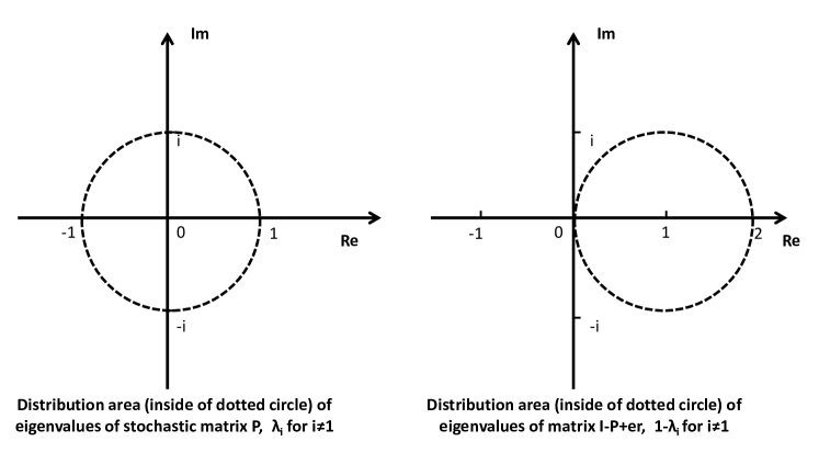
Figure 1: The distribution area of eigenvalues of matrix $\bm{P}$ and $\bm{I}-\bm{P}+\bm{e}\bm{r}$, i.e., $\lambda_{i}$ and $1-\lambda_{i}$ for $i\neq 1$.

Therefore, we can directly derive the following theorem.

Theorem 2.

The matrix $\bm{I}-\bm{P}+\bm{e}\bm{r}$ is not singular if and only if $\bm{r}\bm{e}\neq 0$, where $\bm{P}$ is the stochastic matrix of an irreducible and aperiodic Markov chain.

Proof.

The proof of this theorem is very straightforward. Based on Theorem 1 and Lemma 2, we see that the eigenvalues of $\bm{I}-\bm{P}+\bm{e}\bm{r}$ are either $\bm{r}\bm{e}$ or $1-\lambda_{i}$ for $i\neq 1$. Since $\bm{r}\bm{e}\neq 0$ and $|\lambda_{i}|<1$ for $i\neq 1$, we can easily verify that $0$ is not the eigenvalue of $\bm{I}-\bm{P}+\bm{e}\bm{r}$. Therefore, the matrix is invertible and the theorem is proved. ∎

With Theorem 2, we see that $\bm{I}-\bm{P}+\bm{e}\bm{r}$ is invertible if $\bm{r}\bm{e}\neq 0$. Therefore, we define a generalized fundamental matrix as below.

$$\bm{Z_{r}}:=(\bm{I}-\bm{P}+\bm{e}\bm{r})^{-1},\qquad\bm{r}\bm{e}\neq 0.$$ (8)

Compared with the fundamental matrix $\bm{Z}^{*}:=(\bm{I}-\bm{P}+\bm{e}\bm{\pi})^{-1}$ defined in the literature [11], $\bm{Z}^{*}$ can be viewed as a special case of $\bm{Z_{r}}$ with $\bm{r}=\bm{\pi}$.

The generalized fundamental matrix $\bm{Z_{r}}$ is an important quantity of Markov chains and it can be utilized to compute the performance potential and the steady state distribution, as we will discuss in the following subsections.

2.2 Computation of Performance Potential

As we know, the value function (or performance potential) is an very important quantity of Markov decision processes. In a standard policy iteration procedure, we have to compute the value function for the current policy, which is called the policy evaluation step [14]. In the approximate dynamic programming, we study various approximation approaches to simplify the computation of the value function to alleviate the curse of dimensionality [2]. Therefore, the efficient computation of the value function is an very important topic in the field of MDPs. Note that the computation of value functions under the discount criterion is easy, because the associated Poisson equation has a unique solution. We focus on the value function under the long-run average criterion of MDPs.

The performance potential is an alias of the value function and it has a special physical meaning from the perspective of the perturbation analysis and the sensitivity-based optimization [4]. In the following content, we will use the term of performance potential to study how to compute or estimate it. We denote the performance potential as an $S$-dimensional column vector $\bm{g}$ and its element $g(i)$, $i\in\mathcal{S}$, is defined as below.

$$g(i):=\lim\limits_{T\rightarrow\infty}E\left\{\sum_{t=0}^{T-1}[f(X_{t})-\eta]|X_{0}=i\right\},$$ (9)

where $X_{t}$ is the system state at time $t$, $f(X_{t})$ is the system reward at state $X_{t}$, and $\eta$ is the long-run average performance defined as below.

$$\eta:=\lim\limits_{T\rightarrow\infty}E\left\{\frac{1}{T}\sum_{t=0}^{T-1}f(X_{t})|X_{0}=i\right\}=\lim\limits_{T\rightarrow\infty}\frac{1}{T}\sum_{t=0}^{T-1}f(X_{t}),$$ (10)

where the second equality holds when the Markov chain is a unichain.

Extending the right-hand side of (9) at time $t=0$ and recursively substituting (9), we can obtain

$$g(i)=f(i)-\eta+\sum_{j\in\mathcal{S}}p(i,j)g(j).$$ (11)

Rewriting the above equation in a matrix form, we obtain the Poisson equation as below.

$$\bm{g}=\bm{f}-\eta\bm{e}+\bm{P}\bm{g}.$$ (12)

The above equation can be rewritten as below.

$$(\bm{I}-\bm{P})\bm{g}=\bm{f}-\eta\bm{e}.$$ (13)

However, as we know from Lemma 2, the matrix $(\bm{I}-\bm{P})$ has an eigenvalue with value 0 and it is not invertible. Noticing the fact that $\bm{g}+c\bm{e}$ is still a solution to (12) for any constant $c$, we can properly choose $c$ to let $\bm{\pi}\bm{g}=\eta$. Therefore, we have

$$(\bm{I}-\bm{P}+\bm{e}\bm{\pi})\bm{g}=\bm{f}.$$ (14)

With Theorem 2, we see that matrix $(\bm{I}-\bm{P}+\bm{e}\bm{\pi})$ is invertible. The inverse matrix is called the fundamental matrix defined in the literature [11] and it has

$$(\bm{I}-\bm{P}+\bm{e}\bm{\pi})^{-1}=\sum_{n=0}^{\infty}(\bm{P}-\bm{e}\bm{\pi})^{n}=\bm{I}+\sum_{n=1}^{\infty}(\bm{P}^{n}-\bm{e}\bm{\pi}).$$ (15)

Therefore, the solution to the Poisson equation (12) can be written as below.

$$\bm{g}=(\bm{I}-\bm{P}+\bm{e}\bm{\pi})^{-1}\bm{f}.$$ (16)

The above formula widely exists in the literature [3, 4] and we can use it to numerically compute the value of $\bm{g}$ for a specific MDP. Note that the value of $\bm{g}$ computed with (16) satisfies the condition $\bm{\pi}\bm{g}=\eta$. However, $\bm{\pi}$ is not a given parameter in the above equation. We have to compute the value of $\bm{\pi}$ before we can use (16) to compute $\bm{g}$. This increases the computation burden. Moreover, if we conduct online estimation, the estimation error of $\bm{\pi}$ may increase the estimation variance of $\bm{g}$.

Fortunately, we have another way to numerically compute $\bm{g}$ without the extra computation for $\bm{\pi}$. Since $\bm{g}+c\bm{e}$ is still a solution to (12) for any constant $c$, for any $S$-dimensional row vector $\bm{r}$ satisfying $\bm{r}\bm{e}\neq 0$, we can choose a proper $c$ to let $\bm{r}\bm{g}=\eta$. Therefore, we can rewrite (12) as below.

$$(\bm{I}-\bm{P}+\bm{e}\bm{r})\bm{g}=\bm{f}.$$ (17)

Since matrix $(\bm{I}-\bm{P}+\bm{e}\bm{r})$ is always invertible as proved in Theorem 2, the above equation can be further rewritten as

$$\bm{g}=(\bm{I}-\bm{P}+\bm{e}\bm{r})^{-1}\bm{f},$$ (18)

where $\bm{r}$ is any $S$-dimensional row vector $\bm{r}$ satisfying $\bm{r}\bm{e}\neq 0$. We can see that all the parameters in (18) are given and we can directly compute $\bm{g}$ with (18) without any pre-computation.

Remark 1. Both (16) and (18) are solutions to the Poisson equation (12) and they have difference only with a constant column vector $c\bm{e}$. The value of $\bm{g}$ in (16) satisfies $\bm{\pi}\bm{g}=\eta$, while the value of $\bm{g}$ in (18) satisfies $\bm{r}\bm{g}=\eta$.

Remark 2. (16) can be viewed as a special case of (18) if we choose $\bm{r}=\bm{\pi}$. With (18), we have more flexibility to choose different $\bm{r}$’s, which may give some insights on the computation or estimation of $\bm{g}$.

2.3 Computation of Steady State Distribution

The fundamental matrix can also be used to compute the steady state distribution of Markov chains. We also assume that the Markov chain is irreducible and aperiodic. We know that $\bm{\pi}$ can be determined by the following set of linear equations

$$\begin{array}[]{l}\bm{\pi}\bm{P}=\bm{\pi}.\\ \bm{\pi}\bm{e}=1.\end{array}$$ (19)

We can rewrite the above equations according to the standard form of linear equations as below.

$$\begin{array}[]{l}(\bm{I}-\bm{P}^{T})\bm{\pi}^{T}=\bm{0}.\\ \bm{e}^{T}\bm{\pi}^{T}=1.\end{array}$$ (20)

That is,

$$\left[\left(\begin{array}[]{ccccc}1&0&0&\cdots&0\\ 0&1&0&\cdots&0\\ 0&0&1&\cdots&0\\ \vdots&\vdots&\vdots&\ddots&\vdots\\ 0&0&0&\cdots&1\\ \end{array}\right)-\left(\begin{array}[]{ccccc}P_{1,1}&P_{2,1}&P_{3,1}&\cdots&P_{S,1}\\ P_{1,2}&P_{2,2}&P_{3,2}&\cdots&P_{S,2}\\ P_{1,3}&P_{2,3}&P_{3,3}&\cdots&P_{S,3}\\ \vdots&\vdots&\vdots&\ddots&\vdots\\ P_{1,S}&P_{2,S}&P_{3,S}&\cdots&P_{S,S}\\ \end{array}\right)\right]\left(\begin{array}[]{c}\pi_{1}\\ \pi_{2}\\ \pi_{3}\\ \vdots\\ \pi_{S}\\ \end{array}\right)=\left(\begin{array}[]{c}0\\ 0\\ 0\\ \vdots\\ 0\\ \end{array}\right).$$ (21)

$$\pi_{1}+\pi_{2}+\pi_{3}+\dots+\pi_{S}=1.$$ (22)

For any $S$-dimensional row vector $\bm{r}$ satisfying $\bm{r}\bm{e}\neq 0$, we multiply $r(i)$ on both sides of (22) and summate this equation to the $i$th equation of (21), $i=1,2,\cdots,S$. We can obtain

$$(\bm{I}-\bm{P}^{T}+\bm{r}^{T}\bm{e}^{T})\bm{\pi}^{T}=\bm{r}^{T}.$$ (23)

With Theorem 2, we know that $\bm{I}-\bm{P}^{T}+\bm{r}^{T}\bm{e}^{T}$ is invertible and $(\bm{I}-\bm{P}^{T}+\bm{r}^{T}\bm{e}^{T})^{-1}=\bm{Z}^{T}_{\bm{r}}$. Therefore, we have

$$\bm{\pi}^{T}=(\bm{I}-\bm{P}^{T}+\bm{r}^{T}\bm{e}^{T})^{-1}\bm{r}^{T},$$ (24)

or

$$\bm{\pi}=\bm{r}(\bm{I}-\bm{P}+\bm{e}\bm{r})^{-1},\qquad\bm{r}\bm{e}\neq 0.$$ (25)

From the above equation, we can see that the computation of $\bm{\pi}$ has the same key part as the computation of $\bm{g}$ with (18), i.e., the computation of the generalized fundamental matrix $\bm{Z_{r}}=(\bm{I}-\bm{P}+\bm{e}\bm{r})^{-1}$. Therefore, $\bm{Z_{r}}$ plays a key role in the analysis of Markov chains.

2.4 Property Analysis and Estimation Algorithm

In this subsection, we discuss the properties of the generalized fundamental matrix $\bm{Z_{r}}$ and the effect on the computation of performance potentials. If the spectral radius of $\bm{P}-\bm{e}\bm{r}$ is smaller than 1, we can rewrite the generalized fundamental matrix as follows.

$$\bm{Z_{r}}=\sum_{n=0}^{\infty}(\bm{P}-\bm{e}\bm{r})^{n},\qquad\rho(\bm{P}-\bm{e}\bm{r})<1.$$ (26)

According to Lemma 1, we see that the eigenvalues of $\bm{P}-\bm{e}\bm{r}$ are $\lambda_{1}-\bm{r}\bm{e}$ and $\lambda_{i}$ for $i\neq 1$, where $\lambda_{i}$ are the eigenvalues of $\bm{P}$ sorted in the descending order of their modulus. With Lemma 2, we see that $\lambda_{1}=1$ and $|\lambda_{i}|<1$ for $i\neq 1$. Therefore, we have

$$\rho(\bm{P}-\bm{e}\bm{r})<1\quad\Longleftrightarrow\quad 0<\bm{r}\bm{e}<2.$$ (27)

Furthermore, we can verify that (26) can be rewritten as below.

$$\bm{Z_{r}}=\sum_{n=0}^{\infty}\left[\bm{P}^{n}-\bm{e}\bm{r}\sum_{j=0}^{n-1}(1-\bm{r}\bm{e})^{j}\bm{P}^{n-1-j}\right],\qquad 0<\bm{r}\bm{e}<2.$$ (28)

If we choose $\bm{r}$ such that $\bm{r}\bm{e}=1$, then we can further simplify the above equation as below.

$$\bm{Z_{r}}=\sum_{n=0}^{\infty}\left[\bm{P}^{n}-\bm{e}\bm{r}\bm{P}^{n-1}\right],\qquad\bm{r}\bm{e}=1,$$ (29)

where we define $\bm{e}\bm{r}\bm{P}^{n-1}=0$ when $n=0$. If we choose $\bm{r}$ stochastic, then the $(i,j)$’th entry of $(\bm{I}-\bm{P}+\bm{e}\bm{r})^{-1}$ has the interpretation that it is a sum over $n$ in which the $n$’th term (for $n\geq 1$) is $P(X_{n}=j|X_{0}=i)-P(X_{n-1}=j|X_{0}$ having initial distribution $\bm{r}$). If we manipulate the terms in the summation of (29), we can obtain

$$\bm{Z_{r}}=\sum_{n=0}^{\infty}\left[\bm{P}^{n}-\bm{e}\bm{r}\bm{P}^{n}\right]+\lim\limits_{n\rightarrow\infty}\bm{e}\bm{r}\bm{P}^{n},\qquad\bm{r}\bm{e}=1.$$ (30)

Since the Markov chain is irreducible, aperiodic, and finite, the limiting probability exists and it equals the steady state distribution. That is,

$$\lim\limits_{n\rightarrow\infty}\bm{P}^{n}=\bm{e}\bm{\pi}.$$ (31)

Therefore, the above equation (30) can be rewritten as below.

$$\bm{Z_{r}}=\sum_{n=0}^{\infty}\left[\bm{P}^{n}-\bm{e}\bm{r}\bm{P}^{n}\right]+\bm{e}\bm{\pi},\qquad\bm{r}\bm{e}=1.$$ (32)

Therefore, neglecting the steady distribution $\bm{e}\bm{\pi}$ for simplicity, we can see that the $n$’th term of the above summation is $P(X_{n}=j|X_{0}=i)-P(X_{n}=j|X_{0}$ having initial distribution $\bm{r}$). This interpretation can help develop online estimation algorithms for quantities related to $\bm{Z_{r}}$ from a viewpoint of sample paths.

Substituting (32) into (18), we have

$$\bm{g} = (\bm{I}-\bm{P}+\bm{e}\bm{r})^{-1}\bm{f}$$ (33)

$$= \sum_{n=0}^{\infty}\left[\bm{P}^{n}-\bm{e}\bm{r}\bm{P}^{n}\right]\bm{f}+\bm{e}\bm{\pi}\bm{f}$$

$$= \sum_{n=0}^{\infty}\bm{P}^{n}\bm{f}-\bm{e}\bm{r}\sum_{n=0}^{\infty}\bm{P}^{n}\bm{f}+\eta\bm{e},$$

where $\bm{r}\bm{e}=1$ and $\bm{r}\bm{g}=\eta$. Since $\bm{g}+c\bm{e}$ is still a performance potential for any constant $c$, we can neglect the term $\eta\bm{e}$ in the above equation and rewrite it as below.

$$\bm{g}=\sum_{n=0}^{\infty}\bm{P}^{n}\bm{f}-\bm{e}\bm{r}\sum_{n=0}^{\infty}\bm{P}^{n}\bm{f},$$ (34)

where $\bm{r}\bm{e}=1$ and $\bm{r}\bm{g}=0$.

From the above equation, we can see that $\sum_{n=0}^{\infty}\bm{P}^{n}\bm{f}$ equals the expectation of the accumulated rewards along the sample path, i.e., $\mathbb{E}\{\sum_{t=0}^{\infty}f(X_{t})\}$. We denote

$$\tilde{\bm{g}}=\sum_{n=0}^{\infty}\bm{P}^{n}\bm{f}=\mathbb{E}\left\{\sum_{t=0}^{\infty}f(X_{t})\right\}.$$ (35)

or

$$\tilde{\bm{g}}_{T}=\mathbb{E}\left\{\sum_{t=0}^{T}f(X_{t})\right\},$$ (36)

for a large constant $T$. We can rewrite (34) as below.

$$\bm{g}=\tilde{\bm{g}}-\bm{e}\bm{r}\tilde{\bm{g}}.$$ (37)

When $\bm{r}$ is a probability distribution, the physical meaning of the above equation is that: we sum all the rewards along the sample path, then we use a weighting vector $\bm{r}$ to obtain a reference level $\bm{r}\tilde{\bm{g}}$, the gap between $\tilde{\bm{g}}$ and the reference level $\bm{r}\tilde{\bm{g}}$ is exactly the performance potential (this is also the reason that we call it relative value function).

The insight for the estimation algorithm is that we can just sum all the rewards along the sample path, then we choose an arbitrary reference level determined by a combination of elements of $\tilde{\bm{g}}$, the gap between them is the estimate of performance potentials. This can help to simplify the online estimation procedure. $\bm{r}=\bm{\pi}$ is one of the special cases. For example, we can also set $\bm{r}=(1,0,0,\cdots,0)$, which lets $\tilde{g}(1)$ as the reference level.

Instead of numerically computing $\bm{g}$ with (18), we can further develop an iterative algorithm to estimate the value of $\bm{g}$ based on (18). With (18), we have

$$\bm{g}=\bm{f}-\bm{e}\bm{r}\bm{g}+\bm{P}\bm{g}.$$ (38)

Suppose $\hat{\bm{g}}$ is an unbiased estimate of $\bm{g}$, i.e., $E(\hat{\bm{g}})=\bm{g}$. We have

$$E(\hat{\bm{g}})=\bm{f}-\bm{e}\bm{r}E(\hat{\bm{g}})+\bm{P}E(\hat{\bm{g}}).$$ (39)

Rewriting the above equation as a sample path version, we derive the following equation that holds from the sense of statistics

$$E[\hat{g}(X_{t})] = E[f(X_{t})-\bm{r}\hat{\bm{g}}+\hat{g}(X_{t+1})]$$ (40)

$$= E[f(X_{t})]-\sum_{i\in\mathcal{S}}r(i)E[\hat{g}(i)]+E[\hat{g}(X_{t+1})].$$

Based on the above equation, we develop a least-squares algorithm that can online estimate $\bm{g}$ based on sample paths. Define a quantity $z_{t}$ as below, which can be viewed as the new information learned from the current feedback of the system.

$$z_{t}:=f(X_{t})-\sum_{i\in\mathcal{S}}r(i)\hat{g}(i)+\hat{g}(X_{t+1})-\hat{g}(X_{t}).$$ (41)

With a stochastic approximation framework, we have the following formula to update the value of $\hat{g}$

$$\hat{g}(X_{t})\leftarrow\hat{g}(X_{t})+\alpha_{t}z_{t},$$ (42)

where $\alpha_{t}$ is a positive step-size that satisfies the convergence condition of Robbins-Monro stochastic approximation, i.e.,

$$\sum_{t=0}^{\infty}\alpha_{t}=\infty,\quad\sum_{t=0}^{\infty}\alpha^{2}_{t}<\infty.$$ (43)

or $\alpha_{t}$ satisfies an even looser condition as below [5].

$$\sum_{t=0}^{\infty}\alpha_{t}=\infty,\quad\lim\limits_{t\rightarrow\infty}\alpha_{t}\rightarrow 0.$$ (44)

The name of least-squares of update formula (42) comes from the fact that we aim to obtain the following estimate of $\bm{g}$ that can obtain the least squares of $z_{t}$ in statistics, i.e.,

$$\bm{g}=\operatorname*{argmin}\limits_{\hat{\bm{g}}}E\{z^{2}_{t}\}$$ (45)

The idea of least-squares update formula (42) is similar to that of temporal-difference (TD) algorithm in reinforcement learning [19]. Below, we give a procedure framework of the online estimation algorithm as illustrated in Fig. 2. In Fig. 2, the algorithm stopping criterion can be set as the norm of two successive estimates is smaller than a given small threshold $\epsilon$, i.e., $\parallel\bm{g}-\bm{g}^{\prime}\parallel<\epsilon$, or just simply stop the algorithm after reaching a large step number $T$, i.e., $t>T$.

Initialize $\hat{g}(s)$ arbitrarily, e.g., set $\hat{g}(s)=0$ for all $s\in\mathcal{S}$. Repeat (for each time step $t$): observe the current state $s$, the current reward $f_{t}$, and the next state $s^{\prime}$ calculate $z_{t}=f_{t}-\sum_{s\in\mathcal{S}}r(s)\hat{g}(s)+\hat{g}(s^{\prime})-\hat{g}(s)$ update $\hat{g}(s)\leftarrow\hat{g}(s)+\alpha_{t}z_{t}$ $s\leftarrow s^{\prime}$; $t\leftarrow t+1$ Until a stopping criterion is satisfied.

Figure 2: An online least-squares algorithm to estimate $\bm{g}$ based on (18).

3 Extension to Other Cases

In the previous section, we discuss the generalized fundamental matrix for the discrete time Markov chain. In this section, we extend the result to other cases, including the continuous time Markov process and the Q-factors in reinforcement learning.

3.1 Continuous Time Markov Process

Consider a continuous time Markov process with transition rate matrix $\bm{B}$. Assume the Markov process is ergodic, we can similarly prove

Theorem 3.

The eigenvalue of matrix $\bm{B}$ has the following property: $\lambda^{B}_{1}=0$ is a simple eigenvalue and the associated column eigenvector is $\bm{x}^{B}_{1}=\bm{e}$; $|\lambda^{B}_{i}+\gamma|<\gamma$ for $i\neq 1$, where $\gamma$ is any constant satisfying $\gamma\geq\max_{s}|B(s,s)|$.

Proof.

By using the uniformization technique in MDPs, we can define a matrix $\bm{P}$ as below.

$$\bm{P}:=\bm{I}+\frac{\bm{B}}{\gamma}.$$ (46)

Obviously, $\bm{P}$ is a stochastic matrix since it satisfies $\bm{P}\bm{e}=\bm{e}$ and all of its elements are nonnegative. The statistical behavior of the Markov chain with transition probability matrix $\bm{P}$ is equivalent to that of the Markov process with transition rate matrix $\bm{B}$ [14]. We have

$$\bm{B}=\gamma(\bm{P}-\bm{I}).$$ (47)

Since the Markov process with $\bm{B}$ is ergodic, the equivalent Markov chain with $\bm{P}$ is also ergodic. Therefore, $\bm{P}$ is an ergodic stochastic matrix. With Lemma 2, we know that the eigenvalue of $\bm{P}$ has

$$\left\{\begin{array}[]{ll}\lambda^{P}_{i}=1,&i=1;\\ |\lambda^{P}_{i}|<1,&i\neq 1;\\ \end{array}\right.$$ (48)

Therefore, with (47), we see that the eigenvalue of $\bm{B}$ is $\lambda^{B}_{i}=\gamma(\lambda^{P}_{i}-1)$ and the column eigenvector is $\bm{x}^{B}_{i}=\bm{x}^{P}_{i}$, $\forall i$. We have

$$\left\{\begin{array}[]{lll}\lambda^{B}_{i}=0,&\bm{x}^{B}_{i}=\bm{e},&i=1;\\ |\lambda^{B}_{i}+\gamma|<\gamma,&\bm{x}^{B}_{i}=\bm{x}^{P}_{i},&i\neq 1;\\ \end{array}\right.$$ (49)

The theorem is proved. ∎

With the above theorem, we know that the eigenvalue of $\bm{B}$ is either $0$ or distributed inside of the dotted circle in Fig. 3. When $\gamma$ is smaller, we can obtain a tighter area describing the distribution area of $\lambda^{B}_{i}$. Obviously, the smallest value of $\gamma$ is

$$\gamma=\max_{s\in\mathcal{S}}|B(s,s)|.$$

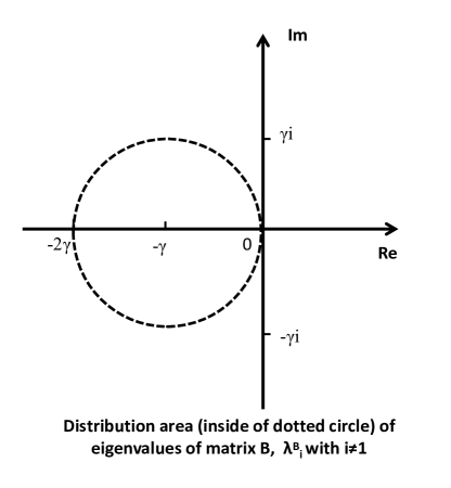
Figure 3: The distribution area of eigenvalues of matrix $B$, i.e., $\lambda^{B}_{i}$ for $i\neq 1$.

Furthermore, we study the eigenvalue of matrix $\bm{D}:=\bm{B}+\bm{e}\bm{r}$ and we can similarly obtain the following theorem.

Theorem 4.

The eigenvalue of matrix $\bm{D}:=\bm{B}+\bm{e}\bm{r}$ has the following property: $\lambda^{D}_{1}=\bm{r}\bm{e}$ is a simple eigenvalue and the associated column eigenvector is $\bm{x}^{D}_{1}=\bm{e}$; $\lambda^{D}_{i}=\lambda^{B}_{i}$ and the associated column eigenvector is $\bm{x}^{D}_{i}=\bm{x}^{B}_{i}+\frac{\bm{r}\bm{x}^{B}_{i}}{\lambda^{B}_{i}-\bm{r}\bm{e}}\bm{e}$ for $i\neq 1$ and $\lambda^{B}_{i}\neq\bm{r}\bm{e}$.

Proof.

The proof of this theorem is similar to that of Theorem 1. We only need to verify whether the eigenvalue and eigenvector satisfy the equation $\bm{D}\bm{x}^{D}_{i}=\lambda^{D}_{i}\bm{x}^{D}_{i}$. Such verification is easy and we ignore the details for simplicity. ∎

Theorem 5.

For any row vector $\bm{r}$ satisfying $\bm{r}\bm{e}\neq 0$, the matrix $\bm{D}:=\bm{B}+\bm{e}\bm{r}$ is invertible, where $\bm{B}$ is the transition rate matrix of an ergodic Markov process.

Proof.

Based on Theorem 3 and Theorem 4, we can easily verify that the eigenvalues of $\bm{D}$ satisfy:

$$\left\{\begin{array}[]{ll}\lambda^{D}_{i}=\bm{r}\bm{e},&i=1;\\ |\lambda^{D}_{i}+\gamma|<\gamma,&i\neq 1;\\ \end{array}\right.$$ (50)

Therefore, $0$ is not the eigenvalue of the matrix $\bm{D}$ and $\bm{D}$ is invertible. ∎

With Theorem 5, we can also simplify the computation of the steady state distribution and the performance potential (value function) of Markov processes.

First, we discuss how to compute the steady state distribution $\bm{\pi}$ in Markov processes. It is known that $\bm{\pi}$ can be determined by the following equations

$$\begin{array}[]{ll}\bm{\pi}\bm{B}=\bm{0}\\ \bm{\pi}\bm{e}=1\\ \end{array}$$ (51)

Multiplying $r(i)$ on both sides of the second equation and adding it to the $i$th row of the first equation, we can obtain the following equation after proper manipulations

$$\bm{\pi}(\bm{B}+\bm{e}\bm{r})=\bm{r}.$$ (52)

With Theorem 5, for any $S$-dimensional row vector $\bm{r}$ satisfying $\bm{r}\bm{e}\neq 0$, $(\bm{B}+\bm{e}\bm{r})$ is invertible and we have

$$\bm{\pi}=\bm{r}(\bm{B}+\bm{e}\bm{r})^{-1},\qquad\bm{r}\bm{e}\neq 0.$$ (53)

Second, we discuss how to compute the performance potential of Markov processes. In a continuous time Markov process, the performance potential $\bm{g}$ is defined as below.

$$g(i)=\lim\limits_{T\rightarrow\infty}E\left\{\int^{T}_{0}[f(X_{t})-\eta]dt\Big{|}X_{0}=i\right\}.$$ (54)

We also have the Poisson equation for the above definition

$$-\bm{B}\bm{g}=\bm{f}-\eta\bm{e}.$$ (55)

In the literature, it is widely adopted that $\bm{g}$ can be numerically computed by the following equation [3, 4]

$$\bm{g}=-(\bm{B}-\bm{e}\bm{\pi})^{-1}\bm{f}.$$ (56)

The above equation includes the condition $\bm{\pi}\bm{g}=\eta$. Similar to the case of discrete time Markov chain, we can also derive

$$(\bm{B}+\bm{e}\bm{r})\bm{g}=-\bm{f},$$ (57)

where the condition $\bm{r}\bm{g}=\eta$ is required. With Theorem 5, for any $S$-dimensional row vector $\bm{r}$ satisfying $\bm{r}\bm{e}\neq 0$, $(\bm{B}+\bm{e}\bm{r})$ is invertible and we have

$$\bm{g}=-(\bm{B}+\bm{e}\bm{r})^{-1}\bm{f},\qquad\bm{r}\bm{e}\neq 0.$$ (58)

Therefore, we can directly compute the value of $\bm{g}$ using the above equation, without the pre-computation of $\bm{\pi}$ required by (56).

On the other hand, we can also develop an online least-squares algorithm to estimate $\bm{g}$ based on sample paths, which is similar to the algorithm described in Fig. 2 for the case of discrete time Markov chains. For simplicity, we ignore the details.

3.2 Poisson Equation for Q-factors

It is well known that we have Poisson equation for the performance potential or the value function in MDPs. Similar to the performance potential quantifying the effect of the initial state on the average performance, the Q-factor is an important quantity in reinforcement learning and it quantifies the effect of the state-action pair on the system average performance. Below, we give a Poisson equation for Q-factors in an MDP under the time average criterion.

Suppose the current policy is $\mathcal{L}$. In this subsection, all the quantities of MDPs are assumed for the policy $\mathcal{L}$ by default, unless we have specific other notations. The Q-factor of the Markov system under this policy $\mathcal{L}$ is defined as below.

$$Q^{\mathcal{L}}(s,a):=f(s,a)-\eta^{\mathcal{L}}+\sum_{s^{\prime}\in\mathcal{S}}p(s,a,s^{\prime})g^{\mathcal{L}}(s^{\prime}),$$ (59)

where $p(s,a,s^{\prime})$ is the probability of which the system transits from the current state $s$ to the next state $s^{\prime}$ if the action $a$ is adopted.

For a randomized policy, $\mathcal{L}$ is a mapping $\mathcal{L}:\mathcal{S}\rightarrow\Omega(\mathcal{A})$, where $\Omega(\mathcal{A})$ is the set of probability measurements over the action space $\mathcal{A}$. That is, $\mathcal{L}(s,a)$ is the probability of which action $a$ is adopted at state $s$, $s\in\mathcal{S}$ and $a\in\mathcal{A}$. For the deterministic case, $\mathcal{L}$ is a mapping $\mathcal{L}:\mathcal{S}\rightarrow\mathcal{A}$, i.e., $\mathcal{L}(s)$ indicates the action adopted at state $s$. We can rewrite (59) in a recursive form as below.

$$Q^{\mathcal{L}}(s,a)=f(s,a)-\eta^{\mathcal{L}}+\sum_{s^{\prime}\in\mathcal{S}}p(s,a,s^{\prime})\sum_{a^{\prime}\in\mathcal{A}}\mathcal{L}(s^{\prime},a^{\prime})Q^{\mathcal{L}}(s^{\prime},a^{\prime}).$$ (60)

The above equation is a fixed-point equation for Q-factors, which is similar to the Poisson equation for the performance potential or the value function in the classical MDP theory.

By sorting the element $Q^{\mathcal{L}}(s,a)$ in a vector form, we define an $SA$-dimensional column vector $\bm{Q}^{\mathcal{L}}$ as below.

$$\bm{Q}^{\mathcal{L}}(s):=\left[\begin{array}[]{c}Q^{\mathcal{L}}(s,a_{1})\\ Q^{\mathcal{L}}(s,a_{2})\\ \vdots\\ Q^{\mathcal{L}}(s,a_{A})\end{array}\right],\ \forall s\in\mathcal{S}.\qquad\bm{Q}^{\mathcal{L}}:=\left[\begin{array}[]{c}\bm{Q}^{\mathcal{L}}(1)\\ \bm{Q}^{\mathcal{L}}(2)\\ \vdots\\ \bm{Q}^{\mathcal{L}}(S)\end{array}\right].$$ (61)

With the same order to sort the element $s,a,s^{\prime},a^{\prime}$, we can rewrite (60) in a matrix form as below.

$$\bm{Q}^{\mathcal{L}}=\bm{f}-\eta^{\mathcal{L}}\bm{e}+\bm{P}\bm{L}\bm{Q}^{\mathcal{L}},$$ (62)

where $\bm{Q}^{\mathcal{L}}$ and $\bm{r}$ are column vectors with size $SA$, $\bm{e}$ is a column vector of ones with a proper size (here the size is $SA$), $\bm{P}$ is a stochastic matrix with size $SA\times S$

$$\bm{P}:=\Big{[}\bm{P}((s,a),s^{\prime})\Big{]}_{SA\times S},\quad\bm{P}((s,a),s^{\prime})=p(s,a,s^{\prime}),\ \forall s,s^{\prime}\in\mathcal{S},\ a\in\mathcal{A},$$ (63)

$\bm{L}$ is a stochastic matrix with size $S\times SA$

$$\bm{L}:=\Big{[}\bm{L}(s^{\prime},(s^{\prime},a^{\prime}))\Big{]}_{S\times SA},\quad\bm{L}(s^{\prime},(s^{\prime},a^{\prime}))=\mathcal{L}(s^{\prime},a^{\prime}),\ \forall s^{\prime}\in\mathcal{S},\ a^{\prime}\in\mathcal{A},$$ (64)

where $\bm{L}(s,(s^{\prime},a^{\prime}))=0$ if $s\neq s^{\prime}$. Therefore, most of the elements of $\bm{L}$ is 0 and $\bm{L}$ is a sparse matrix like below

$$\bm{L}=\left[\begin{array}[]{ccccc}\mathcal{L}(1,:)&\bm{0}&\bm{0}&\cdots&\bm{0}\\ \bm{0}&\mathcal{L}(2,:)&\bm{0}&\cdots&\bm{0}\\ \vdots&\vdots&\vdots&\ddots&\vdots\\ \bm{0}&\bm{0}&\bm{0}&\cdots&\mathcal{L}(S,:)\end{array}\right]_{S\times SA}.$$ (65)

If we write $\bm{\mathcal{L}}$ as an $S\times A$ matrix as below.

$$\bm{\mathcal{L}}:=\left[\begin{array}[]{cccc}\mathcal{L}(1,a_{1}),&\mathcal{L}(1,a_{2}),&\cdots,&\mathcal{L}(1,a_{A})\\ \mathcal{L}(2,a_{1}),&\mathcal{L}(2,a_{2}),&\cdots,&\mathcal{L}(2,a_{A})\\ \vdots&\vdots&\ddots&\vdots\\ \mathcal{L}(S,a_{1}),&\mathcal{L}(S,a_{2}),&\cdots,&\mathcal{L}(S,a_{A})\\ \end{array}\right]_{S\times A}.$$ (66)

Then matrix $\bm{L}$ equals the block diagonal of Kronecker product (matrix form of tensor-product) of vector $\bm{e}^{T}$ and matrix $\bm{\mathcal{L}}$, where $\bm{e}^{T}$ is an $S$-dimensional row vector of ones. That is, we have

$$\bm{L}=\operatorname*{diag}(\bm{e}^{T}\otimes\bm{\mathcal{L}})=\left[\begin{array}[]{cccc}\bm{\mathcal{L}}(1,:),&\bm{0},&\cdots,&\bm{0}\\ \bm{0},&\bm{\mathcal{L}}(2,:),&\cdots,&\bm{0}\\ \vdots&\vdots&\ddots&\vdots\\ \bm{0},&\bm{0},&\cdots,&\bm{\mathcal{L}}(S,:)\\ \end{array}\right]_{S\times SA}.$$ (67)

It is easy to verify that

$$\begin{array}[]{l}\bm{L}\bm{e}=\bm{e}.\\ \bm{P}\bm{e}=\bm{e}.\end{array}$$ (68)

Therefore,

$$\bm{P}\bm{L}\bm{e}=\bm{e},$$ (69)

and $\bm{P}\bm{L}$ is still a stochastic matrix that can be denoted as matrix $\bm{\tilde{P}}$ with size $SA\times SA$. That is,

$$\bm{\tilde{P}}:=\bm{P}\bm{L}.$$ (70)

Therefore, we obtain a linear form of (62) as below.

$$(\bm{I}-\bm{\tilde{P}})\bm{Q}^{\mathcal{L}}=\bm{f}-\eta^{\mathcal{L}}\bm{e}.$$ (71)

We can see that for any solution of $\bm{Q}^{\mathcal{L}}$ satisfying (71), $\bm{Q}^{\mathcal{L}}+c\bm{e}$ is still a solution to (71), where $c$ is any constant. Therefore, we can let $\bm{Q}^{\mathcal{L}}$ satisfy

$$\bm{r}\bm{Q}^{\mathcal{L}}=\eta,$$ (72)

where $\bm{r}$ is any $SA$-dimensional row vector satisfying $\bm{r}\bm{e}\neq 0$. Substituting the above equation into (71), we obtain

$$(\bm{I}-\bm{\tilde{P}}+\bm{e}\bm{r})\bm{Q}^{\mathcal{L}}=\bm{f}.$$ (73)

Since $\bm{\tilde{P}}$ is a stochastic matrix, with Theorem 2, we know that $(\bm{I}-\bm{\tilde{P}}+\bm{e}\bm{r})$ is invertible. Therefore, we have the following solution of Q-factors

$$\bm{Q}^{\mathcal{L}}=(\bm{I}-\bm{\tilde{P}}+\bm{e}\bm{r})^{-1}\bm{f},\qquad\bm{r}\bm{e}\neq 0.$$ (74)

Therefore, we obtain the Poisson equation (71) for Q-factors, which is a fixed point equation to solve Q-factors. The closed-form solution of Q-factors is also obtained in (74). Based on these equations, we may also develop numerical computation algorithms or online estimation algorithms for Q-factors, similar to the discussion and algorithms in Subsection 2.4. Recently, the deep reinforcement learning, such as the AlphaGo of Google, is becoming a promising direction of artificial intelligence [18] and the Q-factors are fundamental quantities in reinforcement learning [19], how to efficiently compute, estimate or even represent the Q-factors is an interesting topic that deserves further research efforts.

4 Conclusion

In this paper, we study a generalized fundamental matrix in Markov systems. Different from the fundamental matrix in the classical MDP theory, the generalized fundamental matrix does not require the pre-computation of $\bm{\pi}$ and it can provide a more concise form for the computation of some fundamental quantities in Markov systems. Based on the generalized fundamental matrix, we give a closed-form solution to the Poisson equation and represent the values of performance potentials, steady state distribution, and Q-factors of Markov systems. The new representation of these solutions may shed some light on efficiently computing or estimating these fundamental quantities from a new perspective, which is very important for the performance optimization of Markov decision processes.

References

• [1] A. Berman and R. J. Plemmons, Nonnegative Matrices in the Mathematical Sciences, SIAM, 1994.
• [2] D. P. Bertsekas, Dynamic Programming and Optimal Control, Vol. II, 4th Edition: Approximate Dynamic Programming, Athena Scientific, 2012.
• [3] X. R. Cao and H. F. Chen, โ€œPotentials, perturbation realization, and sensitivity analysis of Markov processes,โ€ IEEE Transactions on Automatic Control, vol. 42, pp. 1382-1393, 1997.
• [4] X. R. Cao, Stochastic Learning and Optimization โ€“ A Sensitivity-Based Approach, New York: Springer, 2007.
• [5] H. F. Chen and W. X. Zhao, Recursive Identification and Parameter Estimation, CRC Press, 2014.
• [6] G. Frobenius, โ€œUber Matrizen aus nicht negativen Elementen,โ€ Sitzungsber. Konigl. Preuss. Akad. Wiss., pp. 456-477, 1912.
• [7] J. J. Hunter, Mathematical Techniques of Applied Probability, Volume 2 โ€“ Discrete Time Models: Techniques and Applications, Academic Press, 1983.
• [8] J. J. Hunter, โ€œSimple procedures for finding mean first passage times in Markov chains,โ€ Asia - Pacific Journal Operational Research, Vol. 24, No. 6, pp. 813-829, 2007.
• [9] J. J. Hunter, โ€œGeneralized inverses of Markovian kernels in terms of properties of the Markov chain,โ€ Linear Algebra and its Applications, Vol. 447, pp. 38-55, 2014.
• [10] J. G. Kemeny, โ€œGeneralization of a Fundamental Matrix,โ€ Linear Algebra and Its Applications, Vol 38, pp. 192-206, 1981.
• [11] J. G. Kemeny and L. J. Snell, Finite Markov Chains, Van Nostrand, New Jersey, 1960.
• [12] C. D. Meyer, โ€œSensitivity of the Stationary Distribution of a Markov Chain,โ€ Journal SIAM Journal on Matrix Analysis and Applications, Vol 15, pp. 715-728, 1994.
• [13] O. Perron, โ€œZur Theorie der Uber Matrizen,โ€ Mathematische Annalen, Vol. 64, No. 2, pp. 248-263, doi:10.1007/BF01449896, 1907.
• [14] M. L. Puterman, Markov Decision Processes: Discrete Stochastic Dynamic Programming, New York: John Wiley & Sons, 1994.
• [15] P. J. Schweitzer, โ€œPerturbation theory and finite Markov chains,โ€ Journal of Applied Probability Vol 5, pp. 401-413, 1968.
• [16] P. J. Schweitzer and K. W. Kindle, โ€œAn iterative aggregation-disaggregation algorithm for solving linear equations,โ€ Journal Applied Mathematics and Computation, Vol. 18, pp. 313-353, 1986.
• [17] E. Seneta, โ€œSensitivity of finite Markov chains under perturbation,โ€ Statistics & Probability Letters 17 (1993) 163-168.
• [18] D. Silver, A. Huang, et al., โ€œMastering the game of Go with deep neural networks and tree search,โ€ Nature, Vol. 529, pp. 484-489, 2016.
• [19] R. S. Sutton and A. G. Barto, Reinforcement Learning, An Introduction, The MIT Press, 1998.