EG Andromedae: A New Orbit and Additional Evidence for a Photoionized Wind

Abstract

We analyze a roughly 20 yr set of spectroscopic observations for the symbiotic binary EG And. Radial velocities derived from echelle spectra are best-fit with a circular orbit having orbital period $P$ = 483.3 $\pm$ 1.6 d and semi-amplitude $K$ = 7.34 $\pm$ 0.07 $\rm km~{}s^{-1}$. Combined with previous data, these observations rule out an elliptical orbit at the 10$\sigma$ level. Equivalent widths of H I Balmer emission lines and various absorption features vary in phase with the orbital period. Relative to the radius of the red giant primary, the apparent size of the H II region is consistent with a model where a hot secondary star with effective temperature $T_{h}\approx$ 75,000 K ionizes the wind from the red giant.

1 INTRODUCTION

Symbiotic stars are interacting binary systems consisting of a red giant primary star, a hotter secondary star, and a surrounding ionized nebula (Allen, 1984; Kenyon, 1986; Belczyński et al., 2000; Corradi et al., 2008). Typical systems have orbital periods ranging from $\sim$ 200 d to several decades, bright emission lines from H I, He I, He II, C IV, [Fe VII], O VI, and other highly ionized species, and occasional 2–3 mag eruptions. The primary is usually on its first ascent of the red giant branch, but some of the primary stars are Mira variables. Most secondary stars are hot white dwarfs powered by material accreted from the red giant wind (e.g., Kenyon & Webbink, 1984; Muerset et al., 1991; Sokoloski et al., 2006). In a few systems, an accreting main sequence (Kenyon et al., 1991) or neutron (Chakrabarty & Roche, 1997; Hinkle et al., 2006) star energizes the nebula.

EG And (HD 4174) is a low excitation symbiotic star, with bright H I, [O III], and [Ne III] optical emission lines superimposed on an M-type absorption spectrum (Wilson, 1950; Kenyon, 1986; Skopal et al., 1991; Munari, 1993). In addition to a strong blue continuum, ultraviolet (UV) spectra show emission lines from He II, C IV, N V, O III, O VI, and Si IV (Stencel, 1984; Oliversen et al., 1985; Vogel, 1991; Crowley et al., 2008). The He II $\lambda$1640 emission line flux and the UV continuum shape suggest a hot component with effective temperature $T_{h}\,\sim\,5-8\,\times 10^{4}$ K (Kenyon, 1985; Muerset et al., 1991; Kolb et al., 2004; Crowley et al., 2008). If the cool primary star is a normal M2 giant (Kenyon & Gallagher, 1983; Oliversen et al., 1985; Kenyon & Fernandez-Castro, 1987; Kenyon et al., 1988; Kenyon, 1988; Fekel et al., 2000), the mass of the secondary star is 0.3–0.5 $M_{\odot}$ (Vogel, 1991; Vogel et al., 1992; Kolb et al., 2004).

Photometric and spectroscopic observations of EG And yield an accurate orbital period of 482–483 d (Kaler & Hickey, 1983; Oliversen et al., 1985; Munari et al., 1988; Vogel, 1991; Skopal et al., 1991; Tomov & Tomova, 1996; Skopal, 1997; Fekel et al., 2000; Skopal et al., 2007; Jurdana-Šepić & Munari, 2010; Skopal et al., 2012). At optical minimum, the red giant occults the hot secondary and the strong emission lines (Stencel, 1984; Vogel, 1991; Crowley et al., 2008). Despite a high quality orbit from optical and infrared absorption lines (Fekel et al., 2000), it is not clear whether the optical variability is due to ellipsoidal variations (Wilson & Vaccaro, 1997), illumination of the red giant photosphere or wind (Skopal et al., 2007; Skopal, 2008; Skopal et al., 2012), or colliding winds from the primary and secondary stars (Walder, 1995; Tomov, 1995; Calabrò, 2014).

Here we describe low and high resolution optical spectra of EG And. With roughly 20 yr of fairly continuous observations, our goal is to refine the orbital parameters and to constrain models for time variations in the emission lines. After a short description of the data acquisition in §2, analysis of SAO radial velocities (§3.1) yields an orbital period of 483.3 $\pm$ 1.3 d, with a semi-amplitude $K_{1}$ = 7.34 $\pm$ 0.07 $\rm km~{}s^{-1}$ for the red giant primary. Combined with previous optical and UV data, the new orbit indicates the binary consists of a 0.35–0.55 $M_{\odot}$ white dwarf and a 1.1–2.4 $M_{\odot}$ red giant at a distance of 400 pc (§3.2). Equivalent widths of the H I Balmer lines and TiO absorption bands show clear evidence for illumination of the red giant wind by the hot secondary (§3.3–3.4). Modest X-ray fluxes suggest the hot white dwarf accretes a small fraction of the red giant wind (§3.5). We conclude with a brief summary (§4).

2 OBSERVATIONS

From 1994 September to 2016 January, P. Berlind, M. Calkins, and other observers acquired 480 low resolution optical spectra of EG And with FAST, a high throughput, slit spectrograph mounted at the Fred L. Whipple Observatory 1.5-m telescope on Mount Hopkins, Arizona (Fabricant et al., 1998). They used a 300 g mm^-1 grating blazed at 4750 $\rm\mathring{A}$, a 3^′′ slit, and a thinned 512 $\times$ 2688 CCD. These spectra cover 3800–7500 $\rm\mathring{A}$ at a resolution of 6 $\rm\mathring{A}$. Spectra are reduced in NOAO IRAF. After trimming the CCD frames at each end of the slit, we correct for the bias level, flat-field each frame, and apply an illumination correction. The full wavelength solution is derived from calibration lamps acquired immediately after each exposure. The wavelength solution for each frame has a probable error of $\lesssim$ $\pm$0.5 $\rm\mathring{A}$. To construct final 1-D spectra, object and sky spectra are extracted using the optimal extraction algorithm apextract within IRAF. Most of the resulting spectra have moderate signal-to-noise, S/N $\gtrsim$ 15–30 per pixel.

On reasonably clear nights, observations of several standard stars enable flux-calibration on the Hayes & Latham (1975) system (see also Barnes & Hayes, 1984; Massey et al., 1988). After an extinction correction using the KPNO extinction curve, the sensitivity curve for each standard is derived using the appropriate tables in the IRAF irscal directory. After calculating the average sensitivity curve for 6–10 standard stars, we apply the flux-calibration to spectra of symbiotic stars. On high quality nights, the calibration has a typical uncertainty of $\pm$0.10 mag ($\pm$0.05 mag) for $\lambda\lesssim$ 4000–4500 $\rm\mathring{A}$ ($\lambda\gtrsim$ 4000–4500 $\rm\mathring{A}$).

Despite the excellent quality of flux-calibration on some nights, many nights were plagued with cirrus or thicker clouds. To measure the long-term variation of absorption and emission features, we measure equivalent widths using sbands within IRAF. In this routine, we define a central wavelength $\lambda_{0}$ for each feature and continuum points on either side of $\lambda_{0}$. After measuring fluxes in 30 $\rm\mathring{A}$ bandpasses at all three wavelengths and interpolating the continuum flux to the central wavelength, the equivalent width is EW = $-2.5$ log ($F_{0}/F_{i}$), where $F_{i}$ is the interpolated continuum flux and $F_{0}$ is the observed flux in a bandpass centered at $\lambda_{0}$. With this definition, absorption (emission) lines yield a positive (negative) equivalent width.

For strong emission features, we derive fluxes using IRAF splot, which performs least-squares fits of a gaussian plus a polynomial. Comparisons with fluxes derived from the equivalent widths suggest a 5% to 10% error. As emission lines become weaker, identifying a robust continuum for the least-squares fit becomes more challenging. The equivalent widths then appear to provide a more consistent measure of the strength of the absorption or emission in each line.

Prior to the start of the FAST observations, we obtained occasional optical spectrophotometric observations of EG And throughout 1982-1989 with the cooled dual-beam intensified Reticon scanner (IRS) mounted on the white spectrograph at the KPNO No. 1 and No. 2 90 cm telescopes. We used NOAO IRAF software to reduce these data to the Hayes & Latham (1975) flux scale; the photometric calibration has an accuracy of $\pm$3–5%.

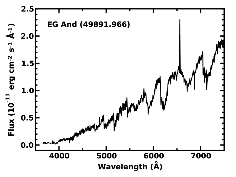
Figure 1: Flux-calibrated optical spectrum of EG And acquired on JD 2449891.966. Aside from strong TiO absorption bands, the system has prominent H$\alpha$ emission and weak H$\beta$ and H$\gamma$ emission features.

Fig. 1 shows a flux-calibrated FAST spectrum for EG And. Aside from extending over a somewhat larger wavelength range, the IRS spectra are identical. Prominent TiO absorption features are visible longwards of $\sim$ 5000 $\rm\mathring{A}$; the Ca I $\lambda$4227 line is also very strong. Low ionization emission lines are visible on many spectra. Aside from H I Balmer lines, weak Fe II, [Fe II], He I, [O III], and [Ne III] are sometimes visible. Higher ionization features often observed in symbiotic stars, such as He II, N III, and [Fe VII], are never visible on FAST or IRS spectra.

Various remote observers acquired high resolution spectroscopic observations of EG And with the echelle spectrographs and Reticon detectors on the 1.5-m telescopes of the Fred L. Whipple Observatory on Mount Hopkins, Arizona and the Oak Ridge Observatory in Harvard, Massachusetts (Latham, 1985). These spectra cover a 44 $\rm{\rm\mathring{A}}$ bandpass centered near 5190 $\rm{\rm\mathring{A}}$ or 5200 $\rm{\rm\mathring{A}}$ and have a resolution of roughly 12 ${\rm km~{}s^{-1}}$. Garcia (1986), Kenyon & Garcia (1986), and Garcia & Kenyon (1988) discuss other details regarding the acquisition and reduction of these data for symbiotic stars.

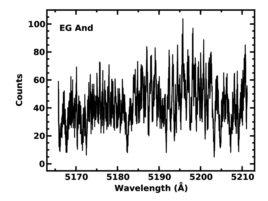
Figure 2: Echelle spectrum of EG And. The strong absorption lines are characteristic of early type M giant stars.

Fig. 2 shows a typical echelle spectrum. The Mg I b and other absorption lines characteristic of M giants are prominent. Although some symbiotic stars have weak iron emission lines at these wavelengths, our EG And spectra never show these features (see also Crowley et al., 2008).

We measure absorption-line radial velocities of the M giant component by cross-correlating EG And spectra against the spectrum of a template star (Tonry & Davis, 1979; Hartmann et al., 1986). All of the EG And spectra were cross-correlated against a very well-exposed spectrum of an M-type giant with velocity derived from cross-correlation against various IAU standard stars and the dusk/dawn sky (e.g., Latham, 1985; Mazeh et al., 1996). This procedure places radial velocities from the two observatories on a common scale with typical errors of 0.75 $\rm km~{}s^{-1}$. After eliminating several spectra compromised by moonlight and cirrus and updating several measurements from Garcia (1986), we have 108 velocities over roughly 14 years of observations (Table 1).

3 ANALYSIS

3.1 Orbital Solution

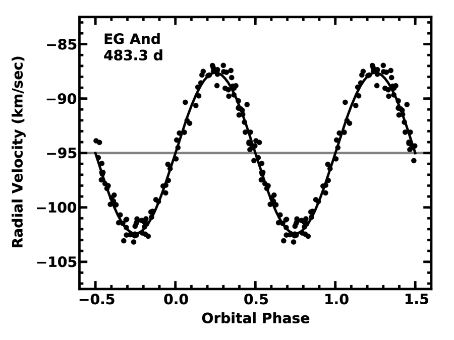
Figure 3: Orbital motion in EG And. Filled circles: SAO radial velocity data. Solid black line: best-fitting solution for circular orbit. Solid horizontal grey line: derived systemic velocity.

We analyze the radial velocity data in Table 1 using the Monet (1979) Fourier transform algorithm as implemented by Kenyon & Garcia (1986). To estimate errors in the orbital parameters, we perform a Monte Carlo simulation. Our approach replaces each velocity measurement $v_{i}$ with $v_{j}=v_{i}+\sigma_{v}r_{j}$, where $\sigma_{v}$ is the error in the original measurement (0.75 $\rm km~{}s^{-1}$) and $r_{j}$ is a gaussian random deviate (Press et al., 1992). We then derive a best-fitting orbital period $P$, semi-amplitude $K$, systemic velocity $\gamma$, projected semimajor axis $a_{1}$, and time of spectroscopic conjunction $T_{0}$. Repeat trials yield a distribution of $N$ values for each orbital parameter. We adopt the median value as ‘best’ and set the dispersion and inter-quartile range for each parameter as the error. In practice, $N=10^{4}$ trials provides a robust estimate of the period; the dispersion and inter-quartile range are fairly indistinguishable. For consistency, we choose the inter-quartile range as the error in each parameter. Fig. 3 plots the data and the orbital solution; Table 2 lists our best estimates and errors for the orbital parameters.

The orbital parameters deduced from the SAO data agree well with previous spectroscopic estimates. For an adopted period $P$ = 482 d, Fekel et al. (2000) quote a semi-amplitude derived from infrared spectra, $K=7.7\pm 0.3$ $\rm km~{}s^{-1}$, which differs little from our $K$ = 7.34 $\pm$ 0.07 $\rm km~{}s^{-1}$ for $P$ = 483.3 $\pm$ 1.6 d. Adding previous observations from the literature (Oliversen et al., 1985; Munari et al., 1988; Munari, 1993), Fekel et al. (2000) quote a final solution with $P$ = 482.57 $\pm$ 0.53 d and $K$ = 7.32 $\pm$ 0.27 $\rm km~{}s^{-1}$ that is nearly identical to our solution.

Because Fekel et al. (2000) infer orbits using a technique which differs from ours, we calculate orbital parameters for published data sets using the Fourier transform algorithm. Table 2 lists results for the Fekel et al. (2000) infrared data (‘Fekel’) and all previous observations (‘OMMF’; Oliversen et al., 1985; Munari et al., 1988; Munari, 1993; Fekel et al., 2000). Within the errors, these solutions agree with those in Table 3 of Fekel et al. (2000). Combining these data with our new velocities, we derive a combined solution (‘All’) which differs little from the solution using SAO data only (‘SAO’).

Iterating all of these solutions in configuration and Fourier space (Kenyon & Garcia, 1986) yields a modest orbital eccentricity $e\approx$ 0.02–0.04 which has a formal 1$\sigma$–2$\sigma$ significance depending on the data set. For the SAO and combined solutions, the Lucy & Sweeney (1971) test rules out an eccentric orbit at the $\gtrsim 10\sigma$ level (see also Bassett, 1978; Lucy, 1989). Thus, the circular orbital solutions listed in Table 2 are strongly preferred (see also the discussions in Wilson & Vaccaro, 1997; Fekel et al., 2000).

Aside from the eccentricity, these solutions are consistent with previous measurements. The orbital periods for the SAO and combined solutions, 482.5–483.3 d, are close to the 482.2 d period inferred from UV eclipses (Vogel, 1991; Vogel et al., 1992). For the combined (SAO) solutions, the time of spectroscopic conjunction, $\rm T_{0}$ = JD 2445384 (JD 2445381) is identical to the epoch of UV photometric minimum, T = JD 2445380 (Vogel, 1991). Our orbital period and time of spectroscopic conjunction also agree well with the period and time of minimum inferred from optical photometry (Skopal, 1997; Wilson & Vaccaro, 1997; Skopal et al., 2007; Jurdana-Šepić & Munari, 2010; Skopal et al., 2012).

3.2 Basic System Parameters

Although previous analyses constrain basic properties of the two stellar components, the new spectroscopic orbit and recent advances in the effective temperature scale for red giants allows us to improve these results. From a detailed analysis of the UV eclipses, Vogel et al. (1992) derive $R_{g}$ = 74 $\pm$ 10 $R_{\odot}$ for the radius of the giant. The observed K-band brightness and J–K color (K = 2.58; J–K = 1.05; e.g., Kenyon & Gallagher, 1983; Kenyon, 1988; Phillips, 2007) and the extinction correction (e.g., Savage & Mathis, 1979; Muerset et al., 1991) then yield an effective temperature, $T_{g}=3730\pm 130$ K (Worthey & Lee, 2011); a bolometric correction at K, BC(K) = $2.7\pm 0.1$ (Worthey & Lee, 2011); an absolute K-band brightness, M${}_{K}=-5.45\pm 0.05$; and a revised distance of 400 $\pm$ 20 pc. The small formal error follows from the adopted $\pm$0.05 error in J–K and the relative insensitivity of the surface brightness of the red giant as a function of gravity and metallicity when log $g\approx$ 0.5–1 and [Fe/H] $\approx$ 0 (see Worthey & Lee, 2011, and references therein).

This revised distance is identical to a previous estimate from Vogel et al. (1992). Although the nominal Hipparcos distance is roughly 700 pc (Kolb et al., 2004; van Leeuwen, 2007), the 1$\sigma$ error in the parallax is only slightly smaller than the parallax. From an analysis of the UV data, Skopal (2005) favors roughly 600 pc. Given the uncertainty in the UV extinction curve and the improvements in bolometric corrections for M-type giants, we favor a distance of 400 pc.

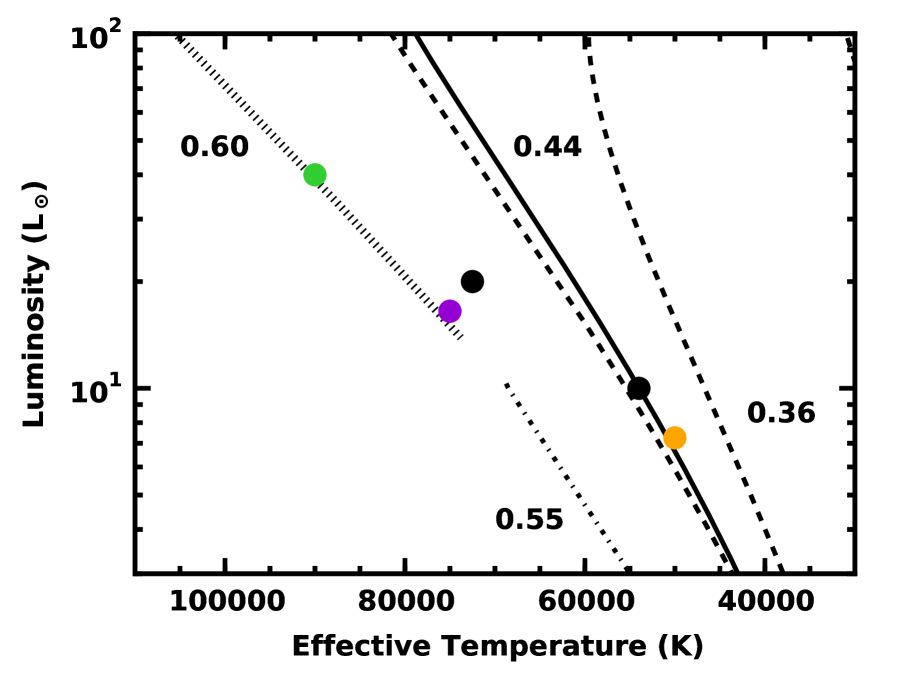
Figure 4: HR diagram for the hot component in EG And. Filled circles indicate published estimates for the effective temperature and luminosity from Kenyon (1985, black), Muerset et al. (1991, purple), Kolb et al. (2004, orange), and Skopal (2005, green). The scatter provides a measure of the uncertainties in the fits to observations of the UV continuum. Black curves plot theoretical tracks (Paczyński, 1971; Salaris et al., 2013; Althaus et al., 2013) for a 0.36 $M_{\odot}$ He white dwarf (dashed lines), a 0.44 $M_{\odot}$ He white dwarf (solid line), a 0.55 $M_{\odot}$ C–O white dwarf (dot-dashed line), and a 0.60 $M_{\odot}$ C–O white dwarf (dotted line). Multiple lines for the 0.36 $M_{\odot}$ white dwarf illustrate the evolution during hydrogen shell flashes.

To estimate the stellar masses, we begin with the position of the hot star in the HR diagram (Fig. 4). Previous analyses suggest hot component effective temperatures $T_{h}\approx$ 50,000–90,000 K (Kenyon, 1985; Muerset et al., 1991; Vogel et al., 1992; Kolb et al., 2004; Skopal, 2005). For a 400 pc distance, the luminosity is then $L_{h}\approx$ 5–40 $L_{\odot}$. The cooler, lower luminosity estimates place the hot component close to white dwarf cooling curves for 0.36–0.44 $M_{\odot}$ He white dwarfs (Althaus et al., 2013). A more luminous hot component falls on cooling curves for 0.55–0.60 $M_{\odot}$ C–O white dwarfs (Paczyński, 1971; Salaris et al., 2013). As indicated by the multiple tracks for the 0.36 $M_{\odot}$ white dwarf in Fig. 4, recurrent hydrogen shell flashes can shift the cooling curves. Given the uncertainties in the observational estimates and the tracks, we adopt a plausible mass range of 0.35–0.55 $M_{\odot}$ for the secondary star.

To constrain properties of the cool primary star, we rely on the derived mass function and Roche geometry. The mass function relates the component masses to the orbital semi-amplitude and the orbital period, $f(M_{g},M_{h})=(a_{1}~{}{\rm sin}~{}i)^{3}/P^{2}$, where $a_{1}~{}{\rm sin}~{}i=KP/2\pi$. In terms of the component masses,

$$f(M_{g},M_{h})\,=\,\frac{(M_{h}\,{\rm sin}\,i)^{3}}{(M_{g}\,+\,M_{h})^{2}}~{}.$$ (1)

When sin $i\approx$ 1, $M_{h}\approx(1+q)^{2}f(M_{g},M_{h})$ where $q=M_{g}/M_{h}$ is the mass ratio. Once $q$ is known, the size of the inner Lagrangian surface sets the maximum radius of the red giant (Eggleton, 1983):

$$R_{g}/a\,\leq\frac{0.49q^{2/3}}{0.6q^{2/3}\,+\,{\rm ln}\,(1\,+\,q^{1/3})}\,,$$ (2)

where $a$ is the semimajor axis, $a=(1+q)a_{1}$.

For $M_{h}\approx$ 0.35–0.55 $M_{\odot}$, the red giant has a modest range of allowed masses (see also Table 2 of Vogel et al., 1992). The derived mass function for the combined set of radial velocities, $f(M_{g},M_{h})$ = 0.019 $\pm$ 0.001, implies $q$ = 3.2–4.4 and $M_{g}\approx$ 1.1–2.4 $M_{\odot}$. As a comparison, radial velocities of the He II $\lambda$1640 emission line suggest $q\approx$ 3.5 (Crowley, 2006). The maximum radius of the red giant ranges from $R_{g,max}\approx$ 185 $R_{\odot}$ for $M_{h}$ = 0.35 $M_{\odot}$ to $R_{g,max}\approx$ 240 $R_{\odot}$ for $M_{h}$ = 0.55 $M_{\odot}$. With an observed radius of roughly 75$R_{\odot}$, the giant fills from 40% ($M_{h}$ = 0.35 $M_{\odot}$) to 30% ($M_{h}$ = 0.55 $M_{\odot}$) of the inner Lagrangian surface. Our estimate for the ratio of the orbital separation to the radius of the red giant, $a/R_{g}\approx$ 3.9–5, compares well with the $a/R_{g}=4.4\pm 0.6$ of Vogel et al. (1992). Given the well-developed red giant wind in EG And (e.g., Vogel et al., 1992; Mikołajewska et al., 2002), the lack of a lobe-filling giant generally agrees with expectations.

3.3 Orbital Modulation of H I emission lines

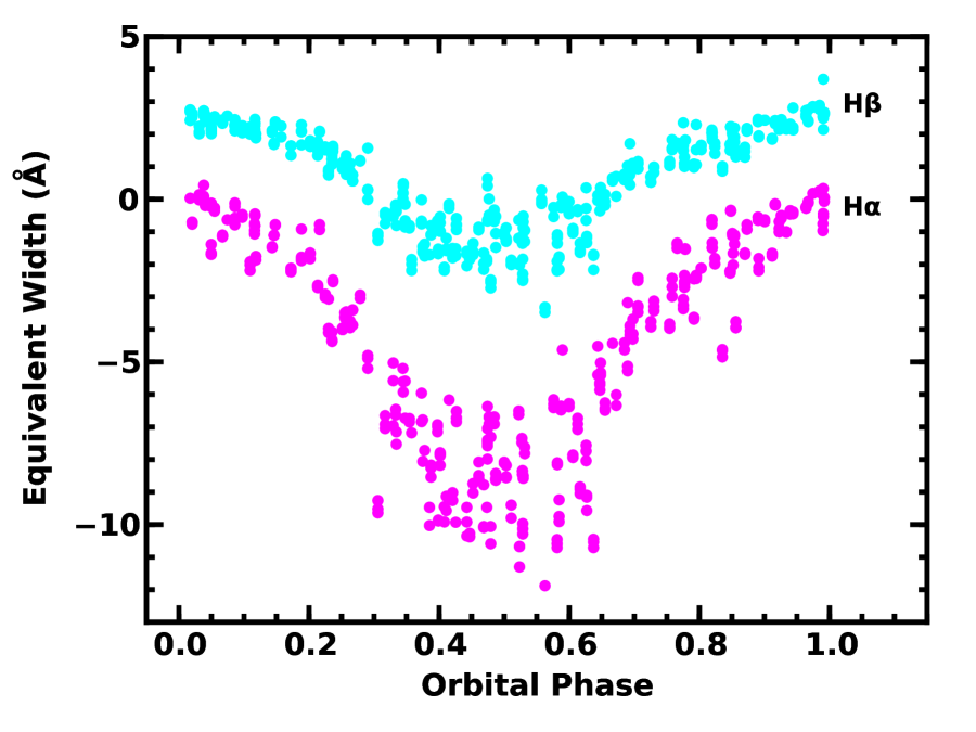
Figure 5: Variation in the measured equivalent widths (EWs) of H$\alpha$ (magenta points) and H$\beta$ (cyan points) as a function of orbital phase. The EWs reach minima at $\phi$ = 0.5, when the illuminated hemisphere and wind of the red giant faces the observer.

To consider the physical structure of the system in more detail, we now examine the FAST observations. Fig. 5 shows the variation of H$\alpha$ and H$\beta$ as a function of orbital phase. Both lines clearly change in phase with the orbit. At spectroscopic conjunctions ($\phi$ = 0), the red giant primary lies in front of the white dwarf secondary. H$\alpha$ is then a weak emission feature superposed on a weak absorption line. The overall EW is zero. As the binary orbits, the emission component gradually strengthens, reaching peak intensity – EW $\approx-10{\rm\mathring{A}}$ – when the red giant lies behind the white dwarf. Following this peak, the emission component gradually weakens until the EW is once again close to zero at $\phi$ = 1.

The H$\beta$ line behaves in a similar fashion. At $\phi$ = 0, the emission component is invisible. The overall EW of 2–3 $\rm\mathring{A}$ is comparable to the typical EW for a normal red giant (O’Connell, 1973; Montes et al., 1997; James, 2013). As the white dwarf moves in front of the red giant, the emission component increases to a maximum intensity with EW $\approx-2~{}{\rm\mathring{A}}$ at $\phi\approx$ 0.5 and then gradually disappears from $\phi\approx$ 0.5 to $\phi\approx$ 1.

Although H$\gamma$ varies in phase with H$\alpha$ and H$\beta$, other emission lines are too weak to establish coherent time variations. Tests with the strongest He I, [O II], and [O III] lines reveal random variations with orbital phase. Additional searches failed to find evidence for consistent, detectable emission from higher ionization features (e.g., He II $\lambda$4686 or [Fe VII] $\lambda$6087).

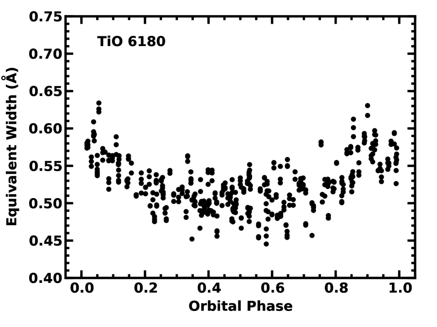
Figure 6: Variation in the measured equivalent width of the TiO $\lambda$6180 absorption band as a function of orbital phase. The absorption is weakest when the illuminated hemisphere of the red giant faces the observer.

Despite this failure, several absorption features clearly change in phase with the orbit. Fig. 6 illustrates the variation of the TiO $\lambda$6180 band. Close to $\phi$ = 0, the absorption line is much stronger (EW $\approx$ 0.55–0.60) than at $\phi\approx$ 0.5 (EW $\approx$ 0.47–0.52). In between these phases, the absorption gradually strengthens and weakens as the binary orbits. Other TiO bands and the prominent Ca I $\lambda$4227 feature similarly vary in phase with the orbit.

3.4 Structure of the Emission Line Region

The time variation of the absorption and emission lines in EG And is qualitatively consistent with the reflection effect. In this interpretation, UV radiation from the hot white dwarf secondary illuminates the facing hemisphere of the red giant primary. The red giant must then emit a larger luminosity with the same surface area, producing a characteristic sinusoidal variation in the optical light curve (e.g., Belyakina, 1968; Kenyon, 1982; Kenyon & Bateson, 1984; Formiggini & Leibowitz, 1990; Skopal, 2008). The large effective temperature of the more luminous hemisphere weakens various absorption features, including the TiO bands. Thus, these absorption features vary in phase with the optical light curve.

Theoretical models (Proga et al., 1996, 1998) demonstrate that high energy photons from the hot secondary in a typical symbiotic can ionize the photosphere and the wind from the red giant. Emission line strengths then depend on the UV luminosity of the secondary and the physical conditions within the red giant wind. For typical parameters, emission line intensities vary in phase with the absorption features and optical light curve, reaching maxima at maximum optical brightness and minimum absorption line strength.

In their analysis of FUSE and HST STIS data for EG And, Crowley et al. (2008) conclude that UV emission lines form close to the hot component. Variability in the emission line profiles suggests that the hot component accretes material from the red giant wind. These data show little or no evidence for a wind from the hot component. Coupled with the sub-Eddington luminosity of the hot component, $L_{h}/L_{edd}\lesssim 10^{-3}$, the UV and EUV data preclude models where colliding winds produce an emission line region between the two stars (e.g., Tomov, 1995; Walder, 1995; Calabrò, 2014).

Adopting parameters for the hot component derived from fits to UV spectra (Muerset et al., 1991) and a density law for the red giant wind (Vogel, 1991), Crowley et al. (2008) derive a predicted structure for the ionized nebula surrounding the hot component. Aside from a tiny He⁺² zone, this model yields a radius of 85–95 $R_{\odot}$ for the size of the H II region. The H II region is then slightly larger than the 65–85 $R_{\odot}$ radius of the M giant. For $E_{B-V}$ = 0.05 (Muerset et al., 1991), the predicted H$\alpha$ flux of $1.0-1.3\times 10^{-10}$ erg cm^-2 s^-1 is within 5%–10% of the maximum flux observed at $\phi$ = 0.5.

The orbital variations of H$\alpha$ and H$\beta$ on FAST spectra are consistent with this picture. In the Crowley et al. (2008) ionization model, we expect to see roughly 20% of the H$\alpha$ emission at mid-eclipse when the giant completely occults the hot component. The FAST observations suggest $|{\rm EW}|\approx$ 1–2 $\rm\mathring{A}$ for H$\alpha$ emission at $\phi\approx$ 0 and 9–11 $\rm\mathring{A}$ at $\phi$ = 0.5. Thus, roughly 10%–20% of the H$\alpha$ emission is visible at mid-eclipse, agreeing with expectations. For H$\beta$, the orbital modulation suggests that 5%–10% of the H II region is visible, consistent with standard photoionization models where H$\alpha$ forms in a slightly larger region than H$\beta$ (e.g., Osterbrock, 1989; Ferland et al., 2013).

Orbit-to-orbit fluctuations in H$\alpha$ and H$\beta$ emission at $\phi$ = 0.5 are also compatible with the FUSE and STIS observations. As discussed in Crowley et al. (2008), variations in the fluxes and profiles of strong emission lines suggest changes in the accretion rate onto the hot component. The FAST observations suggest 20% to 40% fluctuations in H$\alpha$, compared to 20% to 50% variations in the far-UV continuum and emission lines.

Although Crowley et al. (2008) conclude that the hot component has little impact on the absorption spectrum of the red giant, the variations in the TiO absorption index are qualitatively consistent with the ionized wind model. Aside from H$\alpha$, the ionized wind emits Balmer and Paschen continuum radiation (e.g., Osterbrock, 1989). The flux from this component should track the flux from H$\alpha$. Thus, weaker (stronger) H$\alpha$ emission implies a weaker (stronger) Paschen continuum and a stronger (weaker) TiO absorption band, as observed. However, photoionization models predict that the nebula contributes less than 0.01% of the continuum flux at 6000–7000 $\rm\mathring{A}$, much smaller than the amplitude of the variation in the red TiO bands.

Changes in the photospheric temperature of the red giant seem a more likely source of variability in the absorption features. The observed 10% fluctuations in TiO absorption correspond to 0.5 subclass ($\lesssim$ 50 K) changes in the spectral type (effective temperature) of the giant (Kenyon & Fernandez-Castro, 1987). Emission from the hot component and the ionized wind may be sufficient to raise the temperature of the red giant in the hemisphere which faces the hot component (e.g., Proga et al., 1998).

3.5 Disk Accretion

With little evidence for colliding winds in the system, it is worth considering whether the hot white dwarf accretes material from the red giant wind. Based on the shape and time variation of O VI $\lambda\lambda$1032, 1036 line profiles, Crowley et al. (2008) conclude that some accretion is likely. In their analysis of EG And’s X-ray emission, Nuñez et al. (2015) infer an X-ray luminosity, $L_{X}\approx 5\times 10^{-4}{L_{\odot}}$, for optically thin material close to the white dwarf. For a white dwarf with mass $M_{wd}\approx$ 0.4–0.5 $M_{\odot}$, radius $R_{wd}\approx 10^{9}$ cm (Provencal et al., 1998; Holberg et al., 2012), and X-ray luminosity $L_{X}=GM_{wd}\dot{M}_{wd}/2R_{wd}$, an accretion rate $\dot{M}_{wd}\approx 10^{-12}$ ${\rm M_{\odot}~{}yr^{-1}}$ can power the observed X-ray flux. This rate is 0.01% of the mass loss rate of the red giant, $\dot{M}_{g}\approx 10^{-8}{{\rm M_{\odot}~{}yr^{-1}}}$ (Vogel, 1991; Seaquist et al., 1993; Mikołajewska et al., 2002).

To generate this accretion rate, geometric capture is insufficent. Adopting $\dot{M}_{wd}\approx(R_{wd}^{2}/4a^{2})\dot{M}_{g}$, a typical white dwarf radius, and the measured $a$ yields $\dot{M}_{wd}\approx 10^{-17}{{\rm M_{\odot}~{}yr^{-1}}}$. Thus, substantial gravitational focusing is necessary (see also Shore & Wahlgren, 2010; Shagatova et al., 2016).

In the Bondi-Hoyle formalism, disk accretion occurs when the specific angular momentum of accreted material exceeds the specific angular momentum of material orbiting the equator of the white dwarf (e.g., Soker & Rappaport, 2000; Perets & Kenyon, 2013). The accretion rate then depends on the Bondi-Hoyle accretion radius,

$$R_{a}={2GM_{h}\over v_{r}^{2}+c_{s}^{2}},$$ (3)

where $v_{r}$ is the velocity of material near the white dwarf and $c_{s}$ is the sound speed. Adopting a reasonable range for $v_{r}$ = 30–80 $\rm km~{}s^{-1}$ and $c_{s}$ = 10–20 $\rm km~{}s^{-1}$, the accretion rate is then $\dot{M}_{wd}\approx(R_{a}/2a)^{2}\dot{M}_{g}$ $\approx$ 0.003–0.05 $\dot{M}_{g}$ $\approx$ $3-50\times 10^{-11}$ ${\rm M_{\odot}~{}yr^{-1}}$. Even though the red giant fills only 30%–40% of its Roche lobe, the Bondi-Hoyle rate is still 30–500 times larger than the rate required to power the X-ray flux. Thus, accretion can easily power the observed X-ray flux. With a total accretion luminosity of only 0.03–0.5 $L_{\odot}$, however, the energy from Bondi-Hoyle accretion is insufficient to power the observed UV luminosity of the hot white dwarf. More rigorous numerical models (e.g., de Val-Borro et al., 2009) are required to infer the properties of the accreted material in more detail.

4 SUMMARY

Our analysis of optical spectroscopic observations places better constraints on the physical structure of the EG And binary. Roughly 100 new radial velocities yield improved parameters for a circular orbit and eliminate eccentric orbits at the 10$\sigma$ level. Measurements of orbital variations in H$\alpha$ yield a strong test of illumination models, where high energy photons from the hot component ionize the wind from the red giant. When the H$\alpha$ emission line reaches maximum intensity, the observed flux is within 10% of predictions. The small emission flux during the eclipse of the hot component is also consistent with predictions.

Together with an absolute measure of the red giant radius (Vogel, 1991), updated data for effective temperatures and bolometric corrections (Worthey & Lee, 2011) yield a distance, 400 pc, which differs little from previous estimates. For this distance, the luminosity and effective temperature of the hot component are consistent with theoretical models for 0.35–0.55 $M_{\odot}$ He/C–O white dwarfs with H envelopes. The revised spectroscopic mass function then implies a red giant mass $M_{g}\approx$ 1.1–2.5 $M_{\odot}$. The large mass range for the hot component results mainly from factor of roughly 2 uncertainties in the effective temperature and a factor of four uncertainty in the luminosity. Now that H$\alpha$ observations confirm aspects of the illumination model, detailed comparisons between predictions and observations of EUV and UV emission lines might yield better constraints on the effective temperature.

Understanding the orbital modulation of TiO and other strong absorption features requires high resolution spectra covering a large wavelength range (e.g., 3500–8000 $\rm\mathring{A}$). Data at 3500–3800 $\rm\mathring{A}$ might reveal a Balmer emission jump, which could be used to constrain the continuum from the photoionized wind. At longer wavelengths, profile variations in Ca I and other atomic lines along with equivalent width variations in TiO and other molecular bands could establish any variation of effective temperature or gravity around the orbit.

Another uncertainty in the system geometry is the possible ellipsoidal variation of the primary star (Wilson & Vaccaro, 1997). The existence of this variability is somewhat controversial (Walder, 1995; Tomov, 1995; Skopal et al., 2007; Skopal, 2008; Jurdana-Šepić & Munari, 2010; Skopal et al., 2012; Calabrò, 2014). Moreover, light curve fits yield a red giant which fills 85%–97% of its tidal surface; the derived red giant radii, $R_{g}\approx$ 100–230 $R_{\odot}$ for $i\approx$ 45^∘–70^∘, are then much larger than the $R_{g}=74\pm 10$ $R_{\odot}$ inferred from the UV eclipses. A large red giant also seems inconsistent with the existence of a fairly smooth red giant wind and the apparent lack of a large, luminous accretion disk (Vogel, 1991; Kolb et al., 2004). Ellipsoidal light curve analyses on larger sets of optical photometry assuming a more edge-on geometry (80^∘–90^∘) might allow a more consistent solution or completely eliminate this possibility.

In the next few years, Gaia observations will resolve the uncertainties in distance estimates (Lindegren, 2010). For stars as optically bright as EG And with distances smaller than 1 kpc, Lindegren et al. (2012) predict parallaxes with 1% or better accuracy. Once Gaia releases improved distances for EG And and other nearby symbiotics, the luminosities of the hot components will only be sensitive to uncertain effective temperatures. If improved modeling techniques yield smaller uncertainties in the effective temperatures, these distances would enable direct comparisons of the properties of the hot components with theoretical tracks of white dwarfs in the HR diagram.

Table 1: EG And Radial Velocity Data

MJD	Phase	$v_{r}$	O–C		MJD	Phase	$v_{r}$	O–C
45243.7815	0.717	$-$102.51	0.45		48310.4657	0.062	$-$90.34	$-$1.75
45308.5671	0.851	$-$100.90	0.11		48434.8081	0.319	$-$87.58	$-$0.66
45507.8122	0.263	$-$87.76	0.18		48457.8627	0.367	$-$89.04	$-$0.41
45550.7453	0.352	$-$88.07	$-$0.94		48483.6702	0.421	$-$91.45	0.08
45571.8844	0.396	$-$90.83	0.41		48491.7518	0.437	$-$93.09	1.02
45602.8697	0.460	$-$94.12	1.06		48517.7439	0.491	$-$95.70	1.23
45602.8747	0.460	$-$94.01	0.95		48542.8674	0.543	$-$96.94	0.10
46507.4955	0.332	$-$89.19	0.69		48607.4976	0.677	$-$103.07	1.61
46627.8390	0.581	$-$98.01	$-$0.44		48637.5401	0.739	$-$103.18	0.98
46663.7130	0.655	$-$100.69	$-$0.26		48663.4661	0.793	$-$102.35	0.39
46682.7537	0.694	$-$102.54	0.77		48673.4993	0.813	$-$101.55	$-$0.10
46712.5916	0.756	$-$102.55	0.34		48847.7009	0.174	$-$87.50	$-$0.88
46739.7623	0.812	$-$102.46	0.80		48877.7406	0.236	$-$87.13	$-$0.45
46779.5052	0.895	$-$99.46	0.06		48908.5544	0.300	$-$86.95	$-$0.96
46801.5491	0.940	$-$97.96	0.38		48940.6623	0.366	$-$89.66	0.24
46832.4733	0.004	$-$95.54	0.84		48965.6780	0.418	$-$91.07	$-$0.20
46842.5687	0.025	$-$93.17	$-$0.57		48995.4879	0.480	$-$94.40	0.46
46957.8306	0.263	$-$87.34	$-$0.24		49024.4984	0.540	$-$95.96	$-$0.73
47020.7667	0.394	$-$90.21	$-$0.13		49164.8304	0.830	$-$102.65	1.34
47070.6224	0.497	$-$94.35	$-$0.39		49230.7792	0.966	$-$96.44	0.02
47094.7307	0.547	$-$96.78	$-$0.23		49289.7675	0.088	$-$92.27	1.26
47128.5941	0.617	$-$98.87	$-$0.93		49317.6956	0.146	$-$89.75	0.70
47166.4648	0.695	$-$101.10	$-$0.69		49349.6200	0.212	$-$87.84	0.08
47190.4773	0.745	$-$102.61	0.40		49372.5587	0.260	$-$88.81	1.25
47191.5694	0.747	$-$102.45	0.23		49507.8143	0.540	$-$96.79	0.10
47219.5727	0.805	$-$101.34	$-$0.44		49537.8320	0.602	$-$99.13	$-$0.13
47227.4895	0.821	$-$101.50	0.01		49550.8388	0.629	$-$99.76	$-$0.43
47375.8293	0.128	$-$90.64	1.05		49580.7970	0.691	$-$101.14	$-$0.57
47390.8013	0.159	$-$88.56	$-$0.15		49611.7532	0.755	$-$101.48	$-$0.74
47428.7699	0.238	$-$87.48	$-$0.09		49636.7966	0.806	$-$101.79	0.03
47459.7125	0.302	$-$87.53	$-$0.41		49700.6135	0.939	$-$98.67	1.02
47481.6151	0.347	$-$87.42	$-$1.46		49757.4569	0.056	$-$93.10	0.75
47511.5538	0.409	$-$90.95	0.03		49903.8466	0.359	$-$88.86	$-$0.35
47540.5805	0.469	$-$93.09	$-$0.39		49912.7672	0.377	$-$88.82	$-$0.96
47567.4753	0.525	$-$94.03	$-$2.00		49920.7383	0.394	$-$90.88	0.53
47727.8202	0.857	$-$100.36	$-$0.27		49938.8367	0.431	$-$92.17	0.35
47759.7682	0.923	$-$98.04	$-$0.27		49946.7754	0.448	$-$90.55	$-$1.98
47775.8408	0.956	$-$97.52	0.63		49964.8678	0.485	$-$94.49	0.28
47804.7104	0.016	$-$94.51	0.35		49973.7108	0.504	$-$93.88	$-$1.17
47832.5893	0.073	$-$92.02	0.40		49980.6262	0.518	$-$95.43	$-$0.28
47864.5926	0.140	$-$88.95	$-$0.29		50000.7224	0.559	$-$97.82	0.26
47895.5659	0.204	$-$87.89	0.03		50006.7072	0.572	$-$98.26	0.18
47923.4492	0.261	$-$87.44	$-$0.13		50026.6268	0.613	$-$99.43	$-$0.24
48056.8368	0.537	$-$97.47	0.88		50054.6611	0.671	$-$101.47	0.14
48083.8350	0.593	$-$99.72	0.78		50097.4519	0.760	$-$101.06	$-$1.15
48108.8078	0.645	$-$101.41	0.73		50111.5168	0.789	$-$101.20	$-$0.80
48131.8045	0.693	$-$101.85	0.11		50139.4779	0.847	$-$100.42	$-$0.49
48158.7417	0.748	$-$101.73	$-$0.49		50293.7783	0.166	$-$87.83	$-$0.72
48163.7844	0.759	$-$101.33	$-$0.88		50325.6689	0.232	$-$86.96	$-$0.64
48191.6865	0.816	$-$101.05	$-$0.54		50363.7428	0.311	$-$89.05	0.97
48221.5286	0.878	$-$99.29	$-$0.68		50374.7099	0.333	$-$89.78	1.25
48257.6683	0.953	$-$96.04	$-$0.98		50405.6227	0.397	$-$91.51	1.04
48284.4812	0.008	$-$93.81	$-$0.69		50438.5882	0.465	$-$94.69	1.39

Note. — MJD = JD - 2400000, where JD is the Julian Date. The units for $v_{r}$ and O–C are $\rm km~{}s^{-1}$. The orbital phase is the fractional part of $\phi=({\rm JD}-T_{0})/P$, where JD is the Julian Date listed above, $T_{0}$ = JD 2450213.508, and $P$ = 483.3 d.

Table 2: EG And Orbital Solutions

Data Set	$P_{orb}$ (d)	$\gamma$ ($\rm km~{}s^{-1}$)	$K$ ($\rm km~{}s^{-1}$)	$T_{0}$	$a$ sin $i$ (AU)	$f(M)$ ($M_{\odot}$)
All	482.5 $\pm$ 1.3	$-$94.74 $\pm$ 0.09	7.30 $\pm$ 0.13	208.108 $\pm$ 0.672	0.323 $\pm$ 0.003	0.019 $\pm$ 0.001
Fekel	483.2 $\pm$ 13.3	$-$95.18 $\pm$ 0.12	7.66 $\pm$ 0.22	198.797 $\pm$ 4.160	0.340 $\pm$ 0.013	0.023 $\pm$ 0.003
SAO	483.3 $\pm$ 1.6	$-$94.88 $\pm$ 0.05	7.34 $\pm$ 0.07	213.508 $\pm$ 0.961	0.326 $\pm$ 0.003	0.020 $\pm$ 0.001
OMMF	482.7 $\pm$ 1.3	$-$95.01 $\pm$ 0.10	7.28 $\pm$ 0.18	200.768 $\pm$ 1.840	0.323 $\pm$ 0.008	0.019 $\pm$ 0.001

Note. — The time of spectroscopic conjunction is 2450000 + $T_{0}$. Data sets are ‘All’: all published radial velocities, including those in this paper; ‘Fekel’: KPNO data from Fekel et al. (2000); ‘SAO’: data from this paper; and ‘OMMF’: data from Oliversen et al. (1985), Munari et al. (1988), Munari (1993), and Fekel et al. (2000).

References

- Allen (1984) Allen, D. A. 1984, Proceedings of the Astronomical Society of Australia, 5, 369
- Althaus et al. (2013) Althaus, L. G., Miller Bertolami, M. M., & Córsico, A. H. 2013, A&A, 557, A19
- Barnes & Hayes (1984) Barnes, J. V., & Hayes, D. S. 1984, IRS Standard Star Manual (Association of Universities for Research in Astronomy, Tucson, AZ USA)
- Bassett (1978) Bassett, E. E. 1978, The Observatory, 98, 122
- Belczyński et al. (2000) Belczyński, K., Mikołajewska, J., Munari, U., Ivison, R. J., & Friedjung, M. 2000, A&AS, 146, 407
- Belyakina (1968) Belyakina, T. S. 1968, AZh, 45, 139
- Calabrò (2014) Calabrò, E. 2014, Journal of Astrophysics and Astronomy, 35, 69
- Chakrabarty & Roche (1997) Chakrabarty, D., & Roche, P. 1997, ApJ, 489, 254
- Corradi et al. (2008) Corradi, R. L. M., et al. 2008, A&A, 480, 409
- Crowley (2006) Crowley, C. 2006, PhD thesis, School of Physics, Trinity College Dublin, Dublin 2, Ireland (https://www.tcd.ie/Physics/Astrophysics/crowley.php)
- Crowley et al. (2008) Crowley, C., Espey, B. R., & McCandliss, S. R. 2008, ApJ, 675, 711
- de Val-Borro et al. (2009) de Val-Borro, M., Karovska, M., & Sasselov, D. 2009, ApJ, 700, 1148
- Eggleton (1983) Eggleton, P. P. 1983, ApJ, 268, 368
- Fabricant et al. (1998) Fabricant, D., Cheimets, P., Caldwell, N., & Geary, J. 1998, PASP, 110, 79
- Fekel et al. (2000) Fekel, F. C., Joyce, R. R., Hinkle, K. H., & Skrutskie, M. F. 2000, AJ, 119, 1375
- Ferland et al. (2013) Ferland, G. J., et al. 2013, Rev. Mexicana Astron. Astrofis., 49, 137
- Formiggini & Leibowitz (1990) Formiggini, L., & Leibowitz, E. M. 1990, A&A, 227, 121
- Garcia (1986) Garcia, M. R. 1986, AJ, 91, 1400
- Garcia & Kenyon (1988) Garcia, M. R., & Kenyon, S. J. 1988, in IAU Colloq. 103: The Symbiotic Phenomenon, ed. J. Mikolajewska, M. Friedjung, S. J. Kenyon, & R. Viotti, 27
- Hartmann et al. (1986) Hartmann, L., Hewett, R., Stahler, S., & Mathieu, R. D. 1986, ApJ, 309, 275
- Hayes & Latham (1975) Hayes, D. S., & Latham, D. W. 1975, ApJ, 197, 593
- Hinkle et al. (2006) Hinkle, K. H., Fekel, F. C., Joyce, R. R., Wood, P. R., Smith, V. V., & Lebzelter, T. 2006, ApJ, 641, 479
- Holberg et al. (2012) Holberg, J. B., Oswalt, T. D., & Barstow, M. A. 2012, AJ, 143, 68
- James (2013) James, D. J. 2013, PASP, 125, 1087
- Jurdana-Šepić & Munari (2010) Jurdana-Šepić, R., & Munari, U. 2010, PASP, 122, 35
- Kaler & Hickey (1983) Kaler, J. B., & Hickey, J. P. 1983, PASP, 95, 759
- Kenyon (1982) Kenyon, S. J. 1982, PASP, 94, 165
- Kenyon (1985) Kenyon, S. J. 1985, in Astrophysics and Space Science Library, Vol. 113, Cataclysmic Variables and Low-Mass X-ray Binaries, ed. D. Q. Lamb & J. Patterson, 417–423
- Kenyon (1986) —. 1986, The symbiotic stars (Cambridge University Press, Cambridge, UK)
- Kenyon (1988) —. 1988, AJ, 96, 337
- Kenyon & Bateson (1984) Kenyon, S. J., & Bateson, F. M. 1984, PASP, 96, 321
- Kenyon & Fernandez-Castro (1987) Kenyon, S. J., & Fernandez-Castro, T. 1987, AJ, 93, 938
- Kenyon et al. (1988) Kenyon, S. J., Fernandez-Castro, T., & Stencel, R. E. 1988, AJ, 95, 1817
- Kenyon & Gallagher (1983) Kenyon, S. J., & Gallagher, J. S. 1983, AJ, 88, 666
- Kenyon & Garcia (1986) Kenyon, S. J., & Garcia, M. R. 1986, AJ, 91, 125
- Kenyon et al. (1991) Kenyon, S. J., Oliversen, N. A., Mikolajewska, J., Mikolajewski, M., Stencel, R. E., Garcia, M. R., & Anderson, C. M. 1991, AJ, 101, 637
- Kenyon & Webbink (1984) Kenyon, S. J., & Webbink, R. F. 1984, ApJ, 279, 252
- Kolb et al. (2004) Kolb, K., Miller, J., Sion, E. M., & Mikołajewska, J. 2004, AJ, 128, 1790
- Latham (1985) Latham, D. W. 1985, in Stellar Radial Velocities, ed. A. G. D. Philip & D. W. Latham, 21–34
- Lindegren (2010) Lindegren, L. 2010, in IAU Symposium, Vol. 261, IAU Symposium, ed. S. A. Klioner, P. K. Seidelmann, & M. H. Soffel, 296–305
- Lindegren et al. (2012) Lindegren, L., Lammers, U., Hobbs, D., O’Mullane, W., Bastian, U., & Hernández, J. 2012, A&A, 538, A78
- Lucy (1989) Lucy, L. B. 1989, The Observatory, 109, 100
- Lucy & Sweeney (1971) Lucy, L. B., & Sweeney, M. A. 1971, AJ, 76, 544
- Massey et al. (1988) Massey, P., Strobel, K., Barnes, J. V., & Anderson, E. 1988, ApJ, 328, 315
- Mazeh et al. (1996) Mazeh, T., Latham, D. W., & Stefanik, R. P. 1996, ApJ, 466, 415
- Mikołajewska et al. (2002) Mikołajewska, J., Ivison, R. J., & Omont, A. 2002, Advances in Space Research, 30, 2045
- Monet (1979) Monet, D. G. 1979, ApJ, 234, 275
- Montes et al. (1997) Montes, D., Martin, E. L., Fernandez-Figueroa, M. J., Cornide, M., & de Castro, E. 1997, A&AS, 123
- Muerset et al. (1991) Muerset, U., Nussbaumer, H., Schmid, H. M., & Vogel, M. 1991, A&A, 248, 458
- Munari (1993) Munari, U. 1993, A&A, 273, 425
- Munari et al. (1988) Munari, U., Margoni, R., Iijima, T., & Mammano, A. 1988, A&A, 198, 173
- Nuñez et al. (2015) Nuñez, N. E., Nelson, T., Mukai, K., Sokoloski, J. L., & Luna, G. J. M. 2015, ArXiv e-prints
- O’Connell (1973) O’Connell, R. W. 1973, AJ, 78, 1074
- Oliversen et al. (1985) Oliversen, N. A., Anderson, C. M., Slovak, M. H., & Stencel, R. E. 1985, ApJ, 295, 620
- Osterbrock (1974) Osterbrock, D. E. 1974, Astrophysics of gaseous nebulae (W. H. Freeman and Co., San Francisco, CA)
- Osterbrock (1989) —. 1989, Astrophysics of gaseous nebulae and active galactic nuclei (University Science Books, Mill Valley, CA)
- Paczyński (1971) Paczyński, B. 1971, Acta Astron., 21, 417
- Perets & Kenyon (2013) Perets, H. B., & Kenyon, S. J. 2013, ApJ, 764, 169
- Phillips (2007) Phillips, J. P. 2007, MNRAS, 376, 1120
- Press et al. (1992) Press, W. H., Teukolsky, S. A., Vetterling, W. T., & Flannery, B. P. 1992, Numerical recipes in C. The art of scientific computing (Cambridge: University Press, Cambridge, UK)
- Proga et al. (1998) Proga, D., Kenyon, S. J., & Raymond, J. C. 1998, ApJ, 501, 339
- Proga et al. (1996) Proga, D., Kenyon, S. J., Raymond, J. C., & Mikolajewska, J. 1996, ApJ, 471, 930
- Provencal et al. (1998) Provencal, J. L., Shipman, H. L., Høg, E., & Thejll, P. 1998, ApJ, 494, 759
- Salaris et al. (2013) Salaris, M., Althaus, L. G., & García-Berro, E. 2013, A&A, 555, A96
- Savage & Mathis (1979) Savage, B. D., & Mathis, J. S. 1979, ARA&A, 17, 73
- Seaquist et al. (1993) Seaquist, E. R., Krogulec, M., & Taylor, A. R. 1993, ApJ, 410, 260
- Shagatova et al. (2016) Shagatova, N., Skopal, A., & Cariková, Z. 2016, A&A, 588, A83
- Shore & Wahlgren (2010) Shore, S. N., & Wahlgren, G. M. 2010, A&A, 515, A108
- Skopal (1997) Skopal, A. 1997, A&A, 318, 53
- Skopal (2005) Skopal, A. 2005, in Astronomical Society of the Pacific Conference Series, Vol. 330, The Astrophysics of Cataclysmic Variables and Related Objects, ed. J.-M. Hameury & J.-P. Lasota, 463
- Skopal (2008) —. 2008, Journal of the American Association of Variable Star Observers (JAAVSO), 36, 9
- Skopal et al. (1991) Skopal, A., Chochol, D., Vittone, A. A., Blanco, C., & Mammano, A. 1991, A&A, 245, 531
- Skopal et al. (2012) Skopal, A., Shugarov, S., Vaňko, M., Dubovský, P., Peneva, S. P., Semkov, E., & Wolf, M. 2012, Astronomische Nachrichten, 333, 242
- Skopal et al. (2007) Skopal, A., Vaňko, M., Pribulla, T., Chochol, D., Semkov, E., Wolf, M., & Jones, A. 2007, Astronomische Nachrichten, 328, 909
- Soker & Rappaport (2000) Soker, N., & Rappaport, S. 2000, ApJ, 538, 241
- Sokoloski et al. (2006) Sokoloski, J. L., et al. 2006, ApJ, 636, 1002
- Stencel (1984) Stencel, R. E. 1984, ApJ, 281, L75
- Tomov & Tomova (1996) Tomov, N., & Tomova, M. 1996, Information Bulletin on Variable Stars, 4341, 1
- Tomov (1995) Tomov, N. A. 1995, MNRAS, 272, 189
- Tonry & Davis (1979) Tonry, J., & Davis, M. 1979, AJ, 84, 1511
- van Leeuwen (2007) van Leeuwen, F. 2007, A&A, 474, 653
- Vogel (1991) Vogel, M. 1991, A&A, 249, 173
- Vogel et al. (1992) Vogel, M., Nussbaumer, H., & Monier, R. 1992, A&A, 260, 156
- Walder (1995) Walder, R. 1995, in Annals of the Israel Physical Society, Vol. 11, Asymmetrical Planetary Nebulae, ed. A. Harpaz & N. Soker, 248
- Wilson (1950) Wilson, R. E. 1950, PASP, 62, 14
- Wilson & Vaccaro (1997) Wilson, R. E., & Vaccaro, T. R. 1997, MNRAS, 291, 54
- Worthey & Lee (2011) Worthey, G., & Lee, H.-C. 2011, ApJS, 193, 1