Extracting Patterns of Urban Activity
from Geotagged Social Data

Abstract

Data generated on location-based social networks provide rich information on the whereabouts of urban dwellers. Specifically, such data reveal who spends time where, when, and on what type of activity (e.g., shopping at a mall, or dining at a restaurant). That information can, in turn, be used to describe city regions in terms of activity that takes place therein. For example, the data might reveal that citizens visit one region mainly for shopping in the morning, while another for dining in the evening. Furthermore, once such a description is available, one can ask more elaborate questions: What are the features that distinguish one region from another – is it simply the type of venues they host or is it the visitors they attract? What regions are similar across cities?

In this paper, we attempt to answer these questions using publicly shared Foursquare data. In contrast with previous work, our method makes use of a probabilistic model with minimal assumptions about the data and thus relieves us from having to make arbitrary decisions in our analysis (e.g., regarding the granularity of discovered regions or the importance of different features). We perform an empirical comparison with previous work and discuss insights obtained through our findings.

1 Introduction

Cities are massive and complex systems, the organisation of which we often find difficult to grasp as individuals. Those who live in cities get to know aspects of them through personal experiences: from the cramped bar where we celebrate the success of our favorite sports team to the quiet café where we read a book on Sunday morning. As our daily lives become more digitized, those personal experiences leave digital traces, that we can analyse to understand better how we experience our cities.

In this work, we analyze data from location-based social networks with the goal to understand how different locations within a city are associated with different kinds of activity – and to seek similar patterns across cities. To offer an example, we aim to automatically discover a decomposition of a city into (potentially overlapping) regions, such that one region is possibly associated, say, with shopping centers that are active in the morning, while another is associated with dining venues that are active in the evening. We take a probabilistic approach to the task, so as to relieve ourselves from having to make arbitrary decisions about crucial aspects of the analysis – e.g., the number of such regions or the granularity level of the analysis. This probabilistic approach also provides a principled way to argue about the importance of different features for our analysis – e.g., is the separation of regions mostly due to the different categories of venues therein, or is it due to the different visitors they attract?

Our work belongs to the growing field of Urban Computing [1] and shares its motivation. First, as an ever-increasing number of people live in cities [2], understanding how cities are structured is becoming more crucial. Such structure indeed affects the quality of life for citizens (e.g., how much time we spend commuting), influences real-life decisions (e.g., where to rent an apartment or how much to price a house), and might reflect or even enforce social patterns (e.g. segregation of citizens in different regions). Second, switching perspective from the city to the people, the increasing amount of data produced by urban dwellers offer new opportunities in understanding how citizens experience their cities. This understanding opens possibilities to improve the citizens’ enjoyment of cities. For instance, by matching similar regions across cities, we could improve the relevance of out-of-town recommendations for travelers.

The data we use were produced on Foursquare, a popular location-based social network, and provide rich information about the offline activity of users. Specifically, one of the main functionalities of the platform is enabling its users to generate check-ins that inform their friends of their whereabouts. Each check-in contains information that reveals who (which user) spends time where (at what location), when (what time of day, what day of week), and doing what (according to the kind of venue: shopping at a grocery store, dining at a restaurant, and so on). The dataset consists of a total of 11.5 million Foursquare checkins, generated by users around the globe (Section 2.1).

In the rest of the paper, we proceed as follows. For each city in the dataset, we learn a probabilistic model for the geographic distribution of venues across the city. The trained models associate different regions of the city with venues of different description. These venue descriptions are expressed in terms of data features such as the venue category, as well as the time and users of the related check-ins (Section 2.2). From a technical point of view, we employ a sparse-modeling approach [3], essentially enforcing that a region will be associated with a distinct description only if that is strongly supported by data.

Once such a model is learnt for each city in our dataset through an expectation–maximization algorithm (Section 2.3), we examine how features are spatially distributed within a city, illustrating the insights it provides for some of the cities in our dataset (Section 3). Subsequently, we make use of the learnt models and address two tasks.

• The first is to understand which features among the ones we consider are more significant for distinguishing regions in the same city (Section 4). Somewhat surprisingly, we find that who visits a venue has higher distinguishing power than other features (e.g., the category of the venue). This is a finding that is consistent across the cities that we trained a model for.

• The second is to find similar regions across different cities (Section 5). To quantify the similarity of two regions, we define two measures that have a natural interpretation within the probabilistic framework of this work. First, we discuss the properties of each measure, in what cases one would employ each, and describe how one would employ them in an algorithmic search for similar regions across cities. Subsequently, we employ them on our dataset and find that the regions automatically detected in our model provide very well matching regions

Having provided the results of our analysis, we compare our modeling approach to previously used approaches. Our empirical evaluation in Section 6 shows that our approach outperforms previous attempts [4, 5] in terms of predictive performance as well as finding more distinctly described regions.

Finally, we review related work (Section 7), and discuss possible extensions and improvements of our own work in Section 8. Our code and anonymized versions of our dataset will be made publicly available at http://mmathioudakis.github.io/geotopics/ upon publication.

2 Data & Model

2.1 Dataset

Our dataset consists of geo-tagged activity from Foursquare, a popular location-based social network that, as of 2015, claims more than $50$ million users. It enables users to share their current location with friends, rate and review venues they visit, and read reviews of other users. Foursquare users share their activity by generating check-ins using a dedicated mobile application. Each check-in is associated with a web page that contains information about the user, the venue, and other details of the visit. Each venue is also associated with a public web page that contains information about it — notably the city it belongs to, its geographic coordinates and a category, such as Food or Nightlife Spot.

According to Foursquare’s policy, check-ins are private by default, i.e., they become publicly accessible only at the users’ discretion. This is the case, for example, when users opt to share their check-ins publicly via Twitter, a popular micro-blogging platform. We were thus able to obtain Foursquare data by retrieving check-ins shared on Twitter during the summer 2015. In order to have data for the whole year, we add data from a previous work [6] collected in the same way. We did not apply any filtering during data collection, but for the purposes of this work, we focus on the 40 cities with highest volume of check-ins in our data. The code for collecting the data is made publicly available on github.

The data from the 40 selected cities consist of approximately 6.7 million check-ins with 498 thousand unique users, in total. As a post-processing step, we removed the check-ins of users who contributed check-ins at less than five different venues, resulting in 6.3 million check-ins and approximately 284 thousand unique users (i.e. more than 7,000 unique users per city) in our working dataset. Details of the dataset can be found in Table II.

Although our dataset is made of three type of entities (users, checkins, and venues), we take a venue-centric view of the data. Indeed, venues are the entities associated with the largest amount of information and furthermore, we want to analyse how venues are distributed geographically within a city. Specifically, we associate the following information with each venue.

• A geographic location, expressed as a longitude-latitude pair of geographic coordinates.

• The category of the venue, as specified by Foursquare’s taxonomy (e.g., ‘Art Gallery’, ‘Irani Cafe’, ‘Mini Golf’). If more than one categories are associated with one venue, we keep the one that is designated as the ‘main category’.

• A list of all check-ins associated with this venue in the working dataset. Each check-in is a triplet that contains the following data:

  • The unique identifier of the user who performed it;

  • The day of the week when the check-in occurred, expressed as a categorical variable with values Monday, Tuesday, …, Sunday;

  • The time of the day when the check-in occurred, expressed as a categorical variable with values morning, noon, …, late night, defined according to Table I.

According to this view, each venue is a single data point described in terms of five features – namely location, category, users, times of day and days of week, and it takes a list of values for each feature. For the first two – location and category – the size of the list is always $1$ – i.e., each venue is associated with a single location and a single category. Moreover, location values are continuous two-dimensional, while for all other features the values are categorical. For the categorical features, i.e., category, times of day, days of week, and users, we’ll be using the term dimensionality to refer to the number of values they can take. For example, the dimensionality of times of day is always $6$, that of days of week $7$, that of category is about $700$, and that of users has an average of more than $10,000$ within each city in the dataset.

TABLE I: Time of the Day intervals

	morning	noon	afternoon	evening	night	late night
from	6 am	10 am	2 pm	6 pm	10 pm	2 am
to	10 am	2 pm	6 pm	10 pm	2 am	6 am

TABLE II: Number of check-ins and venues for the 18 (out of 40) cities with most data. They cover a large part of the world (Americas, Europe, Middle East and Asia).

City	Check-ins	Venues	City	Check-ins	Venues
Ankara	104,002	16,983	Mexico City	122,561	28,779
Barcelona	213,859	20,353	Moscow	397,008	51,871
Berlin	141,161	18,544	New York	1,007,377	75,721
Chicago	306,296	27,949	Paris	284,776	28,489
Istanbul	578,042	69,008	Rio de Janeiro	47,743	13,394
Izmir	190,303	20,529	San Francisco	432,625	22,384
Kuala Lumpur	147,103	22,594	Seattle	103,575	10,591
London	234,744	26,453	Washington	412,863	20,122
Los Angeles	367,624	36,086	Tokyo	214,493	38,117
For the 40 cities; 6,335,350 Check-ins and 749,097 Venues in total

2.2 Model Definition

Our analysis is based on a generative model that describes the venues we observe in a city. More precisely, each data point generated by the model corresponds to a single venue, and is associated with a list of values for each feature described in Section 2.1.

Remember that our goal is to uncover associations between geographic locations and other features of venues. Such associations are captured as $k$ topics in the model – i.e., each data point is assigned probabilistically to one topic and different topics generate data venues with different distributions of features. As an example, one topic might generate venues (data points) that are located in the south of a city (feature: location) and are particularly popular in the morning (feature: time of the day), while another might generate venues that are located in the north of a city (feature: location) and predominantly restaurants, bars, and night-clubs (feature: category).

Specifically, to generate one data point, the model performs the following steps:

• Select one ($1$) out of $k$ available topics $\{1,2,\ldots,k\}$ according to a multinomial probability distribution $\theta=(\theta_{1},\theta_{2},\ldots,\theta_{k})$. Let the selected topic be $z$.

• Generate a geographic location $loc=(x,y)$ from a bivariate Gaussian distribution with center $c=c_{z}$ and variance matrix $\Sigma=\Sigma_{z}$.

• For the $i$-th categorical feature, generate a list $\mathbf{u}=\mathbf{u_{i}}$ of $N=N_{i}$ items, where $N_{i}$ is specified as input for this data point. Each element in the list is selected randomly with replacement from a set $U=U_{i}=\{u_{1},u_{2},\ldots,u_{m}\}$ according to multinomial probability $\beta=\beta_{z}^{(i)}=\ (\beta_{z}^{i}\,{}_{|1},\beta_{z}^{i}\,{}_{|2},\ldots,\beta_{z}^{i}\,{}_{|m})$, with $\beta_{z}^{i}\,{}_{|j}\geq 0$ and $\sum_{j=1..m}\beta_{z}^{i}\,{}_{|j}=1$.

The model is depicted in the plate diagram of Figure 1. We stress that there is a different multinomial distribution $\beta=\beta_{z}^{(i)}$ for the $z$-th topic and $i$-th feature. We will be using non-subscript notation ($\beta$ instead of $\beta_{z}^{(i)}$) when we might refer to any such distribution vector – and do the same with other notation symbols.

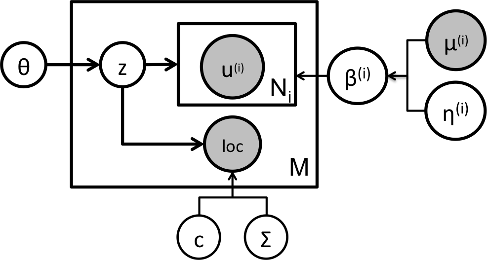
Figure 1: Generative Model. Note that only the $i$-th categorical feature is depicted.

The procedure described above is repeated $M$ times to generate a dataset of size $M$ (i.e., $M$ venues).

Moreover, we assume that, for the $i$-th feature, the probability distribution $\beta_{z}^{i}$ is derived from a probability distribution $\mu^{i}$ and a deviation vector $\eta=\eta_{z}^{i}$ according to the following formula:

$$\beta_{z}^{i}\propto\exp(\mu^{i}+\eta_{z}^{i}).$$ (1)

Firstly, the distribution $\mu$ models the ‘global’ log-probability that the model generate an element $u\in U$. The model makes the assumption that all such probability distributions $\mu^{i}$ are equally likely (uniform prior). Secondly, the deviation vector $\eta_{z}^{i}$ quantifies how much the distribution $\beta_{z}$ of topic $z$ deviates from global distribution $\mu^{i}$. The model makes the assumption that each value of vector $\eta$ is selected at random with prior probability

$$\log p(\eta_{z}^{(i)})=-\lambda\cdot|\eta_{z}^{(i)}|+\text{constant}$$ (2)

for some coefficient $\lambda$, provided as input. The model thus penalizes large deviations from ‘global’ vectors $\mu$, thus leading to ‘sparse’ vectors $\eta_{z}^{i}$. The motivation for favoring sparce vectors $\eta$ is that we wish to associate different topics with different distributions $\beta$ only if we have significant support from the data. For the remaining parameters of the model, we make the following assumptions: all centers $c_{z}$ are equally likely (uniform prior), the value of $\Sigma_{z}$ has a Jeffreys prior,

$$\log p(\Sigma_{z})=-\log\|\Sigma_{z}\|+\text{constant}$$ (3)

and all $\theta$ vectors are equally likely (uniform prior).

2.3 Learning

We learn one instance $I$ of the model for each city in our dataset. Formally, learning corresponds to the optimization problem below.

Problem 1.

Given a set of data points $D=\{d_{1},d_{2},\ldots,d_{{}_{M}}\}$, and the generative model $I$, find global log-probabilities $\mu$, topic distribution $\theta$, deviation vectors $\eta$, bivariate Gaussian centers $c$ and covariances $\Sigma$ that maximize the probability

$$L=p(\{\mu\},\theta,\{\eta\},\{c\},\{\Sigma\}\;|\;D,I).$$

We perform the optimization by partitioning the dataset into a training and test dataset and following a standard validation procedure. During training, we keep $k$ and $\lambda$ fixed and optimize the remaining parameters of the model on the training dataset ($80\%$ of all data points). We then evaluate the performance of the model on the test dataset ($20\%$ of all data points), by calculating the log-likelihood of the test data under the model produced during training. We repeat the procedure for a range of values for $k$ and $\lambda$ to select an optimal configuration.

A max-likelihood vector $\mu$ is computed once for each feature from the raw relative frequencies of observed values of that feature in the dataset. For fixed $k$ and $\lambda$, the maximum-likelihood value of the remaining parameters can be computed with a standard expectation–maximization algorithm. The steps of the algorithms are provided below,

E-Step

$$\log{q_{d}(z)} := \sum_{i=1..m}n_{d}^{(i)}\log{\beta_{z}^{(i)}}+\log{\mathcal{N}(loc_{d};c_{z},\Sigma_{z})}+$$

$$+\log{\theta_{z}}+constant;\;\sum_{z}q_{d}(z)=1$$

M-Step

$$\theta_{z} := \sum_{d\in D}{q_{d}(z)},\;\text{normalized to}\;\sum_{z}\theta_{z}=1$$

$$c_{z} = \frac{\sum_{d}q_{d}(z)\cdot loc_{d}}{\sum_{d}q_{d}(z)}$$

$$\Sigma_{z} := \dfrac{\sum_{d\in D}{q_{d}(z)(loc_{d}-c_{z})(loc_{d}-c_{z})^{T}}}{\sum_{d\in D}{q_{d}(z)}+4}$$

$$\{\eta_{z}^{(i)}\} := \operatorname*{argmax}_{\{\eta_{z}^{(i)}\}}\sum_{d\in D}q_{d}(z)\cdot n_{d}^{(i)}\cdot\log\beta_{z}^{(i)}-\lambda\cdot|\eta_{z}^{(i)}|,$$

with $n_{d}^{(i)}$ the number of times the $i$-th element appears in data point $d$, and the latter optimization (for $\eta$ values) performed numerically.

To optimize with respect to $k$ and $\lambda$, we experiment with a grid of values and select the pair of values with the best performance on the test set. We found that $\lambda\approx 1$ worked well for all cities we experimented with, while improvement reached a plateau for values of $k$ near $k\approx 50-55$. Figure 2 shows the training plots for the city of Paris; similar patterns are observed for the other cities in the dataset.

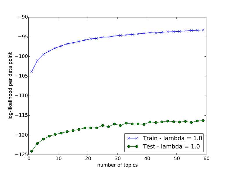
Figure 2: Log-likelihood per data point on the training and test datasets of Paris, for $\lambda=1$ and increasing $k$.

Practical issues

In training, we came across main memory capacity issues during the estimation of model variables related to feature users – particularly for the corresponding multinomial deviation vector $\eta$. We believe that was due to the large dimensionality of the users feature. Indeed, on average, our data contain activity of more than $10,000$ users per city – while the dimensionality of features time of the day, day of the week, category is much lower $6$, $7$, and $\approx 400$, respectively.

To deal with the issue, we use SVD to reduce the dimensionality of feature users. Our goal is to partition the users $\{u_{1},u_{2},\ldots,u_{{}_{M}}\}$ that appear in one city into $d$ groups $U_{1},U_{2},\ldots,U_{d}$, in such a way that $U_{i}$ groups together users that check-in at the same venues. SVD captures nicely such semantics and this property has been used in many settings (e.g., latent semantic indexing [7]). Once the partition is produced, we treat all users in group $U_{i}$, $i=1..d$, as the same user (a ‘super-user’), thus reducing the dimensionality of feature users to $d$.

Specifically, for each city, we consider the users-venue matrix $M$. The $(i,j)$ entry of matrix $M$ contains the number of check-ins observed for the $i$-th user at the the $j$-th venue in the city. Subsequently, we use SVD to compute the $d$ right-eigenvectors $\mathbf{v_{1}},\mathbf{v_{2}},\ldots,\mathbf{v_{d}}$ of $M$. Note that the dimensionality of each such eigenvector $\mathbf{v}$ is equal to the dimensionality of the users feature for a given city. Finally, we partition the users into $d$ groups: we assign the $i$-th user to group $g\in\{0,1,\ldots,d\}$ such that

$$g=\operatorname*{argmax}_{j\in\{1,2,\ldots,d\}}\{\mathbf{v_{1}}[i],\mathbf{v_{2}}[i],\ldots,\mathbf{v_{d}}[i]\}$$

This provides naturally the partition $U_{1},U_{2},\ldots,U_{d}$ we aimed to identify.

3 Likely and distinctive feature values

Following the learning procedure defined in Section 2, we learn a single model for each city in our data. The value of these model instances is that they offer a principled way to answer quesions that we cannot answer from raw data alone. To provide an example, suppose that an acquaintenance from abroad visits our city and asks “if I stay at location $l$ of the city, what is the most common venue category I find there?”. Raw data do not provide an immediate answer to the question. They do allow us, for example, to provide answers of the form “within radius $r$ from $l$, the most common venue category is c with $n$ out of $N$ venues”. However such answers would depend on quantity $r$, that was not provided as input – and would probably never be, if our friend does not have any knowledge about the city. Selecting too small a value for $r$ (e.g., a few meters), would make the answer sensitive to the exact location $l$; selecting too large a value for $r$ (e.g., a few kilometers), would make the answer insensitive to the exact location $l$.

The unsupervised learning approach we take allows us to avoid such arbitrary choices in a principled manner. It learns topics associated with gaussian distributions as regions, whose size is learned from the data; and under a model instance $I$, it allows us to answer our friend’s question by simply considering the probability

$$p(\text{category}=c|\text{location}=l;I)$$

that at the given location we find a venue of category $c$, and answering with the category that is associated with the highest probability value.

Given such model instances, we explore the geographical distribution of venues for the corresponding cities. Due to space constraints, we provide only a few examples here and will provide a complete list of findings from this section on the project’s webpage.

Most likely feature value Suppose a venue is placed at a given location $loc=(x,y)$ – what is the category most likely associated with it? In other words, we are asking for the category that maximizes the expression

$$p(\text{category}=c\;|\;\text{location}=l;I)$$ (4)

that we just discussed above. We use our model to answer this question for New York. The results are shown in Figure 3(a). We can ask a similar question for the remaining categorical features represented in our model. For example, suppose a venue is placed at a given location, what is the most likely time a check-in occurs at that venue? The results for New York are given in Figure 3(b).

Most distinctive feature value Looking again at Figure 3(b), we see that evening check-ins dominate the map: for many locations in Manhattan, a venue placed there is most likely to receive a check-in during the evening. One simple explanation for this is that overwhelmingly many check-ins in our data for this city occur in the evening, as we see in table III.

TABLE III: New York City check-ins in thousands

morning	noon	afternoon	evening	night	latenight
106	219	240	333	118	25

Nevertheless, some areas of the city are more highly associated with morning check-ins than others. In formal terms, for a given location, let us consider the ratio of the probability that the time of day a check-in occurs takes a particular value (‘morning’, ‘noon’, etc) over the probability that a check-in takes that value over the entire city. Arguably, that ratio expresses how distinctive that value is for this particular location. Formally, it is expressed as follows.

$$\frac{p(\text{category}=c\;|\;\text{location}=l;I)}{p(\text{category}=c\;|\;I}$$ (5)

For example, suppose that a venue at a particular location $loc$ receives a check-in in the morning with probability $30$%; and that on average across the city venues, a venue would receive a check-in in the morning with probability only $1\%$. Then, we can say that location $loc$ is associated with venues that are distinguished for the relatively high frequency of morning check-ins. Figure 4(b) indicates the most distinctive time of check-in across New York. We can ask a similar question for other categorical features. For example, what is the most distinctive category for the same location? The results for New York are shown in Figure 4(a).

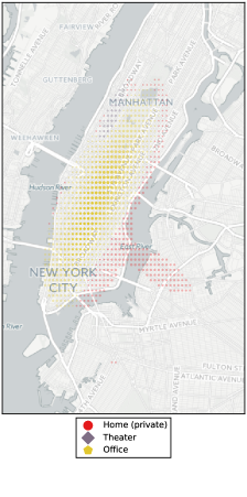
(a) category

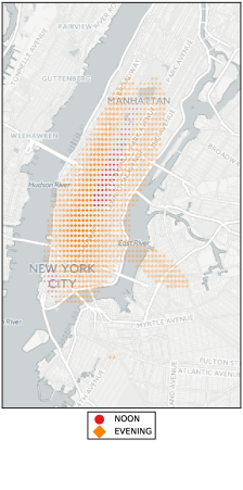
(b) time of day

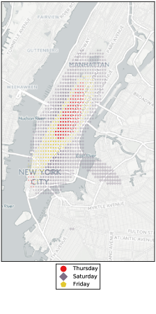
(c) day of week

Figure 3: Most likely category and checkin time of day, day of week across Manhattan. Note that the transparency of each point is equal to the probability that a venue is located at that point.

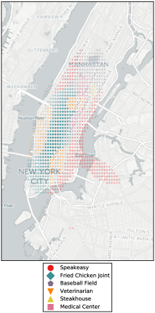
(a) category

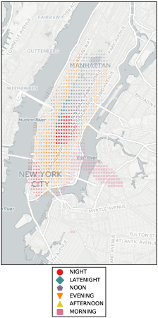
(b) time of day

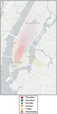
(c) day of week

Figure 4: Most distinctive category and checkin time of day, day of week across Manhattan. The transparency of each point is equal to the probability that a venue is located at that point.

4 Feature analysis

In the previous section, we employed the model instance of a city to ask questions about the geographical distribution of a given feature. In this section, we study the importance of each feature in distinguishing the different topics that define a model instance. To further illuminate the question, let us remember that the model is built upon a set of features $\{X\}$ and that the distribution of each feature is allowed to vary across topics. In plain terms, the question we ask is the following: if we were forced to fix the distribution of feature $X$ across topics, how much would that hurt the predictive performance of the model? This question is important, not just for the purposes of feature selection in case one wanted to employ a simpler model, but also because it allows us to suggest on what features future work should be focused, in order to understand better urban activity.

To be more specific, let us first consider the categorical features in our model: category, users, time of the day, day of the week. Within each topic of a model instance, the distribution $\beta$ of each of the aforementioned features deviates from the overall distribution $\mu$ by a vector $\eta$ (Equation 1). To quantify to which extent a single categorical feature $X$ contributes to the variance across topics, we perform a simple ablation study. That is, we select the same training set as for our best model, keep the value of parameters $k$ and $\lambda$, and train a model instance by fixing the $\eta$ of feature $X$ equal to zero.

$$\text{ for categorical feature}X:\;\text{set}\;\eta=0$$

Subsequently we compare the log likelihood of both models (the best one and the ablated one) over all the data for the given city and measure the log-likelihood drop between the two. The higher this drop, the higher the importance of that feature in explaining the variance across topics.

We perform a similar procedure for the location feature. Specifically, for the ablated model, we replace the bivariate Gaussian distribution $G_{z}$ associated with each model with a distribution $G_{0}$ that remains fixed across topics. $G_{0}$ is set to be the mixture of Gaussians $G_{z}$ across topics $z$, with mixture proportions equal to topic proportions $\theta_{z}$.

$$\text{ for {\tt location}}:\;\text{set}\;G_{0}=\text{mixture}\{G_{z},\theta_{z}\}$$

Results are summarized for all cities in Figure 5. The immediate observation is that users prominently stand out as a feature and that this is consistent across all cities. This suggests that, at least for the urban activity represented in our dataset, who visits a venue has a more important role to play in distinguishing different venues, than where the venues are located and when they are active. Among the remaining features, location and time of the day, are consistently more important across cities than day of the week and category.

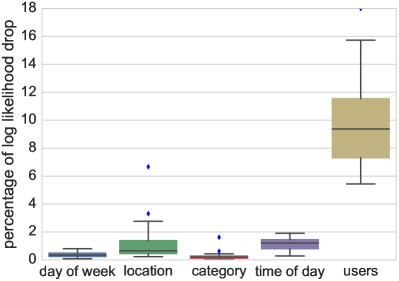
Figure 5: Contribution of each feature to the data likelihood. The boxplots summarize how much the log likelihood drops once we fix the distribution of a single feature across topics. We observe a consistent behavior across cities, in that the variance of users across topics is most important for the predictive performance of the model.

5 Similar regions across cities

In this section, we address the task of discovering similar regions across different cities. Addressing this task would be useful, for example, to generate touristic recommendations for people who visit a foreign city or generally to develop a better understanding of a foreign city based on knowledge from one’s own city. Specifically, we are given the trained models of two (2) cities as input and aim to identify one region from each city so that a similarity measure for the two regions is maximized. Following the conventions of this work, each region is spatially defined in terms of a bivariate Gaussian distribution. Moreover, in the interest of simplicity, we consider only cases where the similarity measure concerns a single feature. In what follows, we present two measures to quantify the similarity of two regions and discuss the merits of each. Subsequently, we argue in favor of one of the two measures, and present an algorithm to find similar regions according to that measure. Finally, we describe some aggregate observations from employing the two measures on our dataset.

5.1 Similarity Measures

We start by defining two similarity measures that have a natural interpretation in our setting. The first one, condsim, quantifies how similar the venues of two regions are on average, according to the corresponding models. The second one, jointsim, combines two qualities of the regions: (i) how similar the venues of two regions are, but also (ii) how many venues they contain, according to the model. The rationale for this second measure is that one might not have a prior idea for how big the two regions should be and at the same time want to avoid identifying pairs of tiny regions that are ‘spuriously’ similar.

5.1.1 Similarity measure condsim

In this section, we define condsim, our first region similarity measure, which operates under the following settings. We are given two model instances, $I_{1}$ and $I_{2}$, each corresponding to a city in our data. As explained in earlier sections of the paper, each model instance describes the distribution of venues in its respective city, along with distributions over every features. Moreover, we are given two bivariate Gaussian distributions, $G_{1}$ and $G_{2}$, each defining one geographic region in the respective model $I_{1}$ and $I_{2}$. To define the similarity between the two regions with respect to feature $X$ (e.g., $X=$ category), we first define a random procedure $\mathcal{P}(I,G,X)$. Given a model instance $I$ and a region $G$, random procedure $\mathcal{P}$ generates one value $X=x$ for feature $X$. It is defined as follows.

Definition 1 ($\mathcal{P}(I,G,X)$).

Perform the following steps.

• Generate a location $l\sim G$.

• Generate a data point at location $l$ from model $I$ and record its value $X=x$ for feature $X$.

• Return value $x$.

In plain terms, random procedure $\mathcal{P}$ picks a random location in region $G$ and then generates a value for feature $X$ according to model instance $I$, conditional on the location selected in region $G$. Similarity measure condsim then answers the question: if random procedure $\mathcal{P}$ is applied on model $I_{1}$ and region $G_{1}$ on one hand, and model $I_{2}$ and region $G_{2}$ on the other, what is the probability that it produces the same value $X=x$ for feature $X$? In other words: if we compare two random venues, one from each region $G_{1}$ and $G_{2}$, what is the probability according to the respective models that they would have the same feature $X$? The measure is formally defined below.

Definition 2 (condsim).

Let $x_{1}$ and $x_{2}$ be the values of feature $X$ generated by a single invocation of $\mathcal{P}(I_{1},G_{1},X)$ and $\mathcal{P}(I_{2},G_{2},X)$, respectively. Similarity condsim is defined as the probability that $x_{1}=x_{2}$.

$${{\tt condsim}}(G_{1},G_{2};I_{1},I_{2},X)=p(x_{1}=x_{2}|\mathbf{P})$$ (6)

We proceed to provide an analytical expression for condsim. First, in the interest of simplicity, we fix model instances $I_{1}$, $I_{2}$ and feature $X$ and write ${{\tt condsim}}(G_{1},G_{2})={{\tt condsim}}(G_{1},G_{2};I_{1},I_{2},X)$. Let us also write $\gamma_{i}(x|l)$ to denote the conditional probability that model $I_{i}$ ($i\in\{1,2\})$, generates a data point at location $l$ with feature $X$ taking value $x$

$$\gamma_{i}(x|l)=p(X=x|loc=l;I_{i}),$$

which can be expanded to

$$\gamma_{i}(x|l)= p(X=x|loc=l;I_{i})$$

$$= \frac{p(X=x,loc=l|I_{i})}{p(loc=l|I_{i})}$$

$$= \frac{\sum_{z=1..k}p(X=x,loc=l,topic=z|I_{i})}{\sum_{z=1..k}p(loc=l,topic=z|I_{i})}$$

$$= \frac{\sum_{z=1..k}{\mathcal{N}_{z}(l)\beta_{z}(v)\theta_{z}}}{\sum_{z=1..k}{\mathcal{N}_{z}(l)\theta_{z}}},$$

where $\mathcal{N}_{z}$ denotes the Gaussian probability density function for the Gaussian distribution associated with the $z$-th topic, $z=1..k$, of model $I_{i}$. Finally, for locations $l_{1}$ and $l_{2}$, let us write $g(l_{1},l_{2})$ for the inner-product function

$$g(l_{1},l_{2})=\sum_{x\in Dom(X)}\gamma_{1}(x|l_{1})\gamma_{2}(x|l_{2}),$$ (7)

where $Dom(X)$ is the set of possible values for feature $X$. With the notational conventions above, we now provide an analytical expression for ${{\tt condsim}}$.

$${{\tt condsim}}(G_{1},G_{2})=\int_{l_{1},l_{2}}\mathcal{N}_{1}(l_{1})\mathcal{N}_{2}(l_{2})g(l_{1},l_{2})dl_{1}dl_{2}$$ (8)

Note that, in equation (8), $\mathcal{N}_{1}$ and $\mathcal{N}_{2}$ denote the probability density functions for Gaussians $G_{1}$ and $G_{2}$, respectively. In practice, we approximate the integral of equation (8) by taking a discrete sum over two $100\times 100$ grids of locations that cover the areas of the corresponding cities.

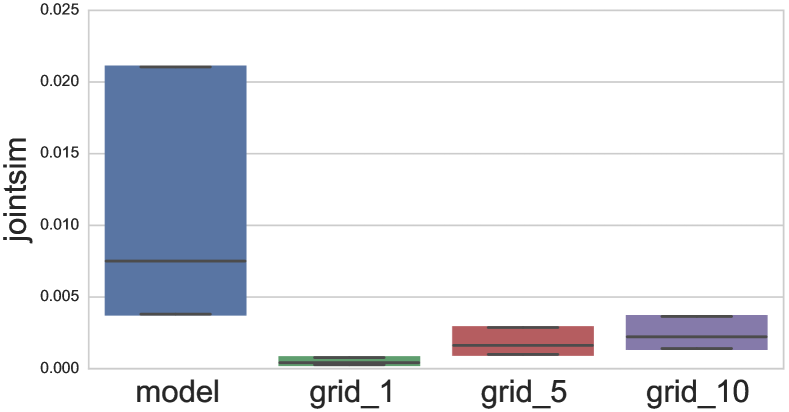
Figure 6: The jointsim values for the best-matching regions returned by GeoExplore across all pairs of cities, for different sets of base-regions (model and grid-$\alpha$).

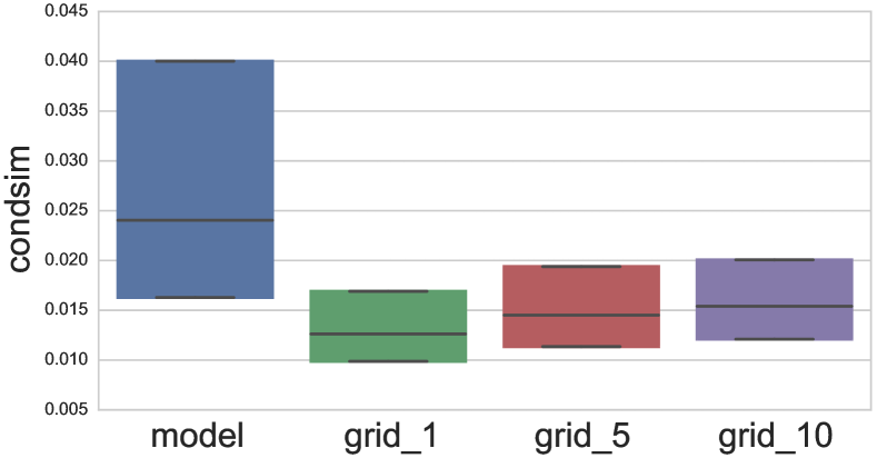
Figure 7: The condsim values for the best-matching regions across all pairs of cities, for different sets of candidate regions (model and grid-$\alpha$).

5.1.2 Similarity measure jointsim

In this section, we define jointsim, our second region similarity measure, which operates under the following settings, similar to that of Section 5.1.1. Namely, we are given two model instances, $I_{1}$ and $I_{2}$, as well as two gaussians $G_{1}$ and $G_{2}$, each defining one region. We define the similarity between the two regions with respect to feature $X$ on top of a random procedure $\mathcal{R}(I,G,X)$, that generates a pair of values $(x,s)$, with $x\in Dom(X)$ and $s\in\mathbb{R}^{+}$. The random procedure $\mathcal{R}$ is defined as follows.

Definition 3 ($\mathcal{R}(I,G,X)$).

Perform the following steps.

• Generate a data point $d\sim I$, with location $loc=l$ and feature $X$ value $X=x$.

• Let $s=\mathcal{N}(l)$ be the probability density of $G$ at location $l$.

• Return the pair $(x,s)$.

In plain terms, random procedure $\mathcal{R}(I,G,X)$ picks a random data point from model instance $I$, and associates it with (1) its value $X=x$ for feature $X$ and (2) the density of region-defining gaussian $G$. Similarity measure jointsim then answers the question: ‘if random procedure $\mathcal{R}$ is applied on model $I_{1}$ and region $G_{1}$, on one hand, and model $I_{2}$ and region $G_{2}$, on the other, with respective output pairs $(x_{1},s_{1})$ and $(x_{2},s_{2})$, what is the expected value of the expression

$$s_{1}\cdot s_{2}\cdot\delta_{x_{1}x_{2}},$$

over possible invocations of procedure $\mathcal{R}$’? In the expression above, $\delta_{x_{1}x_{2}}$ is the Kronecker delta – equal to one ($1$) only when $x_{1}=x_{2}$ and zero ($0$) otherwise. In other words, jointsim combines the answer of the following two questions: if we consider two random venues, one from each model $I_{1}$ and $I_{2}$, then (1) what is the probability that they have the same value for feature $X$, and (2) if they do, how much are their locations covered by regions $G_{1}$ and $G_{2}$? The measure is formally defined below:

Definition 4 (jointsim).

Let $(x_{1},s_{1})$ and $(x_{2},s_{2})$ be the output of a single invocation of random procedure $\mathcal{R}(I_{1},G_{1},X)$ and $\mathcal{R}(I_{2},G_{2},X)$, respectively. Similarity jointsim is defined as the expected value

$${{\tt jointsim}}(G_{1},G_{2};I_{1},I_{2},X)=E_{\mathcal{R}}[s_{1}\cdot s_{2}\cdot\delta_{x_{1}x_{2}}]$$ (9)

We now proceed to provide an analytical expression for jointsim. Following a similar derivation process as in Section 5.1.1, let us write $\psi_{i}(x,l)$ to denote the joint probability that model $I_{i}$ ($i\in\{1,2\}$), generates a data point with feature value $X=x$ and location $l$,

$$\psi_{i}(x|l)=p(X=x,loc=l|I_{i}),$$

with

$$\psi_{i}(x|l)= p(X=x,loc=l;I_{i})$$

$$= p(X=x,loc=l|I_{i})$$

$$= \sum_{z=1..k}p(X=x,loc=l,topic=z|I_{i})$$

$$= \sum_{z=1..k}{\mathcal{N}_{z}(l)\beta_{z}(v)\theta_{z}}$$

Moreover, for locations $l_{1}$ and $l_{2}$, let us write $h(l_{1},l_{2})$ for the inner-product function

$$h(l_{1},l_{2})=\sum_{x\in Dom(X)}\psi_{1}(x,l_{1})\psi_{2}(x,l_{2}).$$ (10)

With the notational conventions above, we now provide an analytical expression for ${{\tt jointsim}}$.

$${{\tt jointsim}}(G_{1},G_{2})=\int_{l_{1},l_{2}}\mathcal{N}_{1}(l_{1})\mathcal{N}_{2}(l_{2})h(l_{1},l_{2})dl_{1}dl_{2}$$ (11)

As in Section 5.1.1, $\mathcal{N}_{1}$ and $\mathcal{N}_{2}$ in equation (8), denote the probability density functions of Gaussians $G_{1}$ and $G_{2}$, respectively. Moreover, we approximate the integral of equation (8) with a discrete sum approximation over a $100\times 100$ grid on each model.

5.1.3 Discussion

Having defined the two similarity measures, let us consider the corresponding maximization problems, first for condsim.

Problem 2.

Consider two models $I_{1}$, $I_{2}$, and feature $X$. Identify two bivariate Gaussians $G_{1}$, $G_{2}$, such that ${{\tt condsim}}(G_{1},G_{2})$ is maximized.

One issue with problem 2 is that it is prone to return spurious regions, i.e., pairs of regions that are very similar, but that cover too small probability mass of the respective models. This can be seen from equations (7) and (8) that define condsim: they take into account the similarity of data points (venues) in terms of feature $X$ at locations within the two regions, but they do not take into account the probability mass that the respective models assign to those regions. To provide a contrived but illuminating example, one can consider the case where $G_{1}$ and $G_{2}$ cover very small areas with few venues that are identical w.r.t. feature $X$. These two regions are thus associated with higher condsim values than larger areas whose venues are similar, but not identical w.r.t. feature $X$. Therefore, if one were to find optimal solutions for Problem 2, they would have to consider such spurious cases as optimal solutions to the problem. Since we have no good way to deal with this issue, we are forced to impose constraints on the possible candidate gaussians $G_{1}$ and $G_{2}$ that comprise the solution pair. Specifically, we consider Problem 3 as a specific case of Problem 2, in which the candidate solution pairs are provided as input.

Problem 3.

Consider two models $I_{1}$, $I_{2}$, and feature $X$. Consider also two collections of Gaussians $\mathbb{G}_{1}$, $\mathbb{G}_{2}$. Identify two bivariate Gaussians $G_{1}\in\mathbb{G}_{1}$, $G_{2}\in\mathbb{G}_{2}$, such that ${{\tt condsim}}(G_{1},G_{2})$ is maximized.

Let us now consider the corresponding optimization problem for jointsim.

Problem 4.

Consider two models $I_{1}$, $I_{2}$, and feature $X$. Identify two bivariate Gaussians $G_{1}$, $G_{2}$, such that ${{\tt jointsim}}(G_{1},G_{2})$ is maximized.

Problem 4 has two intuitive properties:

• all other things being equal, it favors regions $G_{1}$ and $G_{2}$ that cover areas with high probability mass according to models $I_{1}$, $I_{2}$,

• all other things being equal, it favors regions $G_{1}$ and $G_{2}$ that cover areas where data points are associated with similar feature distributions.

To put in plain terms, Problem 4 favors regions that correspond to areas of many and similar data points. This is seen also in equations (10) and (11). Indeed, they take into account the similarity of data points (venues) in terms of feature $X$ at locations within the two regions, but they also take into account the probability mass assigned to those regions by models $I_{1}$ and $I_{2}$. Therefore, Problem 4 does not suffer from the spurious solutions problem that affected Problem 2. This makes Problem 4 appropriate to consider in cases when one does not have prior restrictions or preferences for the candidate regions that would comprise an optimal solution (as in the formulation of Problem 3) and at the same time would like to avoid spurious solutions.

5.2 Best-First Search for Joint Similarity

To the best of our knowledge, the problem of identifying similar regions across cities has not been defined formally before within a probabilistic framework. In this section, we also propose the first algorithm, GeoExplore, to approach Problem 4. Algorithm GeoExplore follows a typical best-first exploration scheme and comprises of the following two phases. Its first phase consists of one step: it begins with a candidate collection of regions $\mathbb{G}_{1}$ and $\mathbb{G}_{2}$ for each side (let us call them ‘base regions’) and evaluates all pairwise similarities ${{\tt jointsim}}(G_{1},G_{2})$, for $G_{1}\in\mathbb{G}_{1}$, $G_{2}\in\mathbb{G}_{2}$. Its second phase consists of the remaining steps: it explores the possibility to improve the currently best jointsim measure by combining previously considered regions. This is motivated by the fact that Problem 4 favors regions of larger probability mass, and therefore combined regions might yield better jointsim values.

Pseudocode for GeoExplore is shown in Algorithm 1. It repeats a three-steps Retrieve - Update - Expand procedure for each step. During Retrieve, the algorithm retrieves the next candidate solution for Problem 4. Each candidate solution comes in the form of a triplet; two Gaussians and their jointsim score. During Update, the algorithm updates the score of the best-matching pair, if a better pair has just been retrieved. Finally, during Expand, the algorithm expands the latest retrieved Gaussians to form Gaussians from each side, and thus new candidate solutions for Problem 4. Subroutine expand(G, I) operates as follows:

• When $G$ is not specified (i.e., $G=\text{NULL}$ in Algorithm 1), then expand simply returns the set of base regions $\mathbb{G}$. This case occurs during the first expansions only. Moreover, each base region $G_{i}\in\mathbb{G}$ is associated with positive weight $w_{i}$, either specified as input, or set to $1/\|\mathbb{G}\|$ by default.

• When $G=G_{i}$ for some $G_{i}\in\mathbb{G}$, then expand returns the set of Gaussians $\{G_{i}\}\bigcup\{G_{i}\cup G_{j};G_{j}\in\mathbb{G},j\neq i\}$, where $G_{i}\cup G_{j}$ is defined as the best Gaussian-fit to the mixture model determined by $[G_{i}$, $G_{j}]$, with respective proportions $(w_{i}$, $w_{j})$. The intuition for this step is that we expand the best-performing pair of Gaussians by combining them with other base Gaussians.

• In a recursive fashion, when $G=G_{i}\cup G_{i^{\prime}}\ldots G_{i^{\prime\prime}}$, then expand returns the set of Gaussians $\{G\}\bigcup\{G\cup G_{j};G_{j}\in\mathbb{G},j\neq i,i^{\prime},\ldots,i^{\prime\prime}\}$ each defined as the best Gaussian-fit to the mixture model determined by $[G$, $G_{j}]$, with respective proportions $(w_{i}+w_{i^{\prime}}+\ldots+w_{i^{\prime\prime}}$, $w_{j})$.

Note that in practice, to prevent the algorithm from exploring the combinatorially large space, we terminate GeoExplore after a number $R$ of while loops.

Algorithm 1 GeoExplore

  Input: models $I_{1}$ and $I_{2}$, base regions $\mathbb{G}_{1}$, $\mathbb{G}_{2}$

  Output: Best Pair $G_{1}$, $G_{2}$

  

  # INITIALIZE

  $\text{BestG}_{1}=\text{NULL}$, $\text{BestG}_{2}=\text{NULL}$,  BestScore = 0

  H = MaxHeap()

  # Initialize max-heap with empty solution, zero score

  Push($\text{BestG}_{1}$, $\text{BestG}_{2}$, BestScore) to H

  

  while H is Not Empty do

     # RETRIEVE top solution in max-heap

     Pop ($\text{G}_{1}$, $\text{G}_{2}$, Score) from H

     # UPDATE best solution

     if Score $>$ BestScore then

        $\text{BestG}_{1}={\text{G}}_{1}$, $\text{BestG}_{2}={\text{G}}_{2}$,  BestScore = Score

     end if

     # EXPAND retrieved solution

     for $\text{G}_{a}$, $\text{G}_{b}$ in expand($\text{G}_{1}$),  expand($\text{G}_{2}$) $\neq\text{G}_{1}$, $\text{G}_{2}$ do

        Score = ${{\tt jointsim}}(G_{a},G_{b}|I_{1},I_{2})$

        Push ($\text{G}_{a}$, $\text{G}_{b}$, Score) to H

     end for

  end while

  return best_pair

5.3 Empirical performance

We employed GeoExplore with $R=5$ expansions on all pairs of cities in our dataset (Section 2.1) and report the jointsim values returned for different base region collections. Specifically, we experimented with the following collections of base regions:

Model

We simply used as collections $\mathbb{G}_{1}$, $\mathbb{G}_{2}$ the Gaussians associated with the respective topics in the input model $I_{1}$, $I_{2}$, and assigned to each Gaussian a weight equal to the respective $\theta$ parameter value found in the model.

Grid-$a$

We used as collections $\mathbb{G}_{1}$, $\mathbb{G}_{2}$ Gaussians that covered in a grid-like fashion the respective cities, each with size equal to $1/a$ the size of the median size of Gaussians found in model $I_{1}$, $I_{2}$.

The results are shown in Figure 6. We observe that using the model Gaussians as our base regions leads to better performance compared with the grid baselines.

Finally, in Figure 7, we report the values obtained for Problem 3 by a straightforward all-pairs algorithm. The collections of Gaussians $\mathbb{G}_{1}$ and $\mathbb{G}_{2}$ provided as input to the problem are defined in the same way as the base regions of Figure 6 above. Again, we observe that we obtain the best performance in terms of condsim when the candidate regions coincide with the model Gaussians.

6 Comparison with previous approaches

In this section, we compare empirically our approach with previous work. Ideally, our comparison would be with works that address the same task as this paper – i.e., model the distribution of venues across a city. In such a case, we would have a natural and direct measure of comparison, namely the predictive performance of each model in terms of log-likelihood. However, to the best of our knowledge, no such work is readily available. Therefore, our comparison is with previous work that addressed slightly different different tasks. Nevertheless, the comparison serves as a ‘sanity check’ for our approach and allows us to understand better the proposed technique.

We compare with two methods which provide publicly available results, namely Livehoods and Hoodsquare. The obtained results concern three large US cities that also appear in our dataset. Both methods use Foursquare data and output a geographical clustering of venues within a city, with each such cluster defining one region on the map of the city. In the case of Livehoods [4], the clusters are obtained through spectral clustering on a nearest-neighbor graph over venues, where the edge weights quantify the volume of visitors who check-in at both adjacent venues. In the case of Hoodsquare [5], clusters are obtained by employing the OPTICS clustering algorithm on venues, using a number of venue features (location, category, peak time of activity during the day, and a binary touristic indicator).

To compare, we perform the following procedure. First, we obtain the clusters returned by each method. We interpret each of those clusters as a region that belongs to one topic, in the sense that we’ve been using the term in the context of our model. To map them to our setting, we approximate the shape of each region with the smallest bivariate Gaussian, so that the entire region is enclosed within two standard deviations of the Gaussian in each direction. (see Figure 8 for the visual results of this approximation in San Francisco) In this way, we obtain a number $k$ of Gaussians from each method. We then train an instance of our model on our data, using the same number $k$ of topics, and keeping the Gaussians associated with each topic fixed to the Gaussians extracted with the aforementioned steps. As in previous sections of the paper, we hold out 20% of the data as test dataset, on which we evaluate the log-likelihood of each learnt model instance.

The log-likelihood achieved by the different models is shown in the first row of Table IV. As one can see there, the results based on our model perform better in predicting the test dataset. This is not surprising, since our approach optimizes predictive accuracy directly. Nevertheless, the results provide evidence that our approach works reasonably well for the task it was designed to address.

To further quantify the differences between the three approaches, we report additional quantities from the learned models, described below. Essentially those quantities capture how distinct the identified regions of each model are in terms of the associated features.

Mean Feature Entropy We consider each categorical feature separately and–for each topic region in the respective model of the three approaches–we measure the entropy of the respective multinomial distribution $\beta$. Intuitively, we would like the regions that constitute our model instances to capture the variance of the various features across the city. Therefore, we would like the $\beta$ distributions of the model instances to have lower entropy (i.e., be farther from uniform). Table IV reports the mean entropy of $\beta$ across regions for each categorical feature and for each of the methods in the three US cities. The relevant lines in the table are the ones labelled ‘mean [feature] entropy’. As one can confirm, in the majority of cases the model instance based on our method returns $\beta$ distributions of lower entropy.

Jensen–Shannon Divergence from City Average Another way to quantify the distinctiveness of the various regions is to measure the distance of the $\beta$ distribution of each feature and topic in the model from the average distribution $\mu$ for the same feature across the city. One principled approach to quantify this difference is to use Jensen–Shannon divergence, ${\rm JSD}(\beta,\mu)$ a symmetrized version of the Kullback–Leibler divergence $\mathrm{KL}(P\parallel Q)$. It is defined with the following formula.

$${\rm JSD}(\beta,\mu)=0.5\cdot\mathrm{KL}(\beta\parallel(\beta+\mu)/2)+0.5\cdot\mathrm{KL}(\mu\parallel(\beta+\mu)/2))$$

Intuitively, it is desirable for $\beta$ distributions of different topics to differ from average city behavior as captured by $\mu$ distributions. Table IV reports the average Jensen–Shannon divergence across the topics for each categorical feature, city, and method. The relevant lines in the table are the ones labelled ‘[feature] JSD from city’. Again, in the majority of cases, the model instance based on our method returns $\beta$ distributions that differ more from city average distribution than the methods we compare with.

To summarize our findings from Table IV, our model has better predictive performance, while generally identifying topic regions that are more distinct with each other and further from average, despite their high overlap. The results thus provide evidence that our approach discovers regions with desirable properties.

TABLE IV: Comparison in San Francisco, New York and Seattle between our model, Livehoods (LH) and Hoodsquare (HS, which has no neighborhoods available in Seattle). The last abbreviation, JSD, stands for the average Jensen–Shannon divergence between regions and city-wide distributions of the four features we consider: category, users, dayOfWeek and timeOfDay. Each group of two adjacent columns is a comparison betwen a competing method and our model. The arrow after the name of each measure indicates whether better values are higher or lower.

		San Francisco				New York				Seattle
		HS	Us	LH	Us	Hoodsquare	Us	Livehoods	Us	Livehoods	Us
likelihood per venue	$\nearrow$	-202.9	-198.3	-197.0	-195.4	-343.9	-277.9	-271.1	-268.2	-112.6	-112.2
mean category entropy	$\searrow$	4.961	4.632	4.802	4.776	4.886	4.714	4.851	4.716	5.178	5.307
category JSD from city	$\nearrow$	0.053	0.092	0.065	0.065	0.054	0.085	0.055	0.070	0.016	0.001
mean dayOfWeek entropy	$\searrow$	1.908	1.894	1.892	1.896	1.923	1.923	1.917	1.917	1.896	1.864
dayOfWeek JSD from city	$\nearrow$	0.007	0.013	0.012	0.012	0.005	0.005	0.006	0.006	0.009	0.016
mean timeOfDay entropy	$\searrow$	1.488	1.440	1.428	1.414	1.522	1.542	1.535	1.535	1.477	1.395
timeOfDay JSD from city	$\nearrow$	0.018	0.034	0.031	0.037	0.018	0.025	0.021	0.024	0.022	0.041
mean users entropy	$\searrow$	5.610	5.617	5.522	5.305	5.929	5.609	5.231	4.975	5.076	5.058
user JSD from city	$\nearrow$	0.160	0.170	0.175	0.201	0.092	0.162	0.198	0.224	0.187	0.192

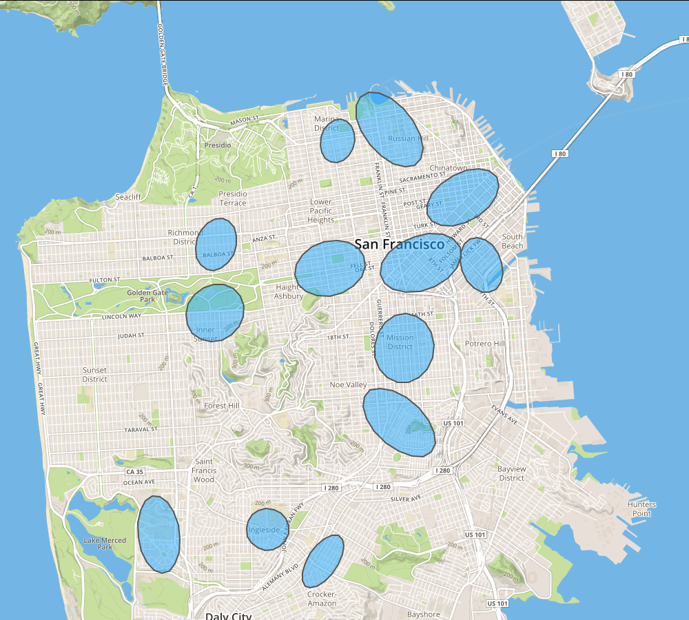
(a) Hoodsquare

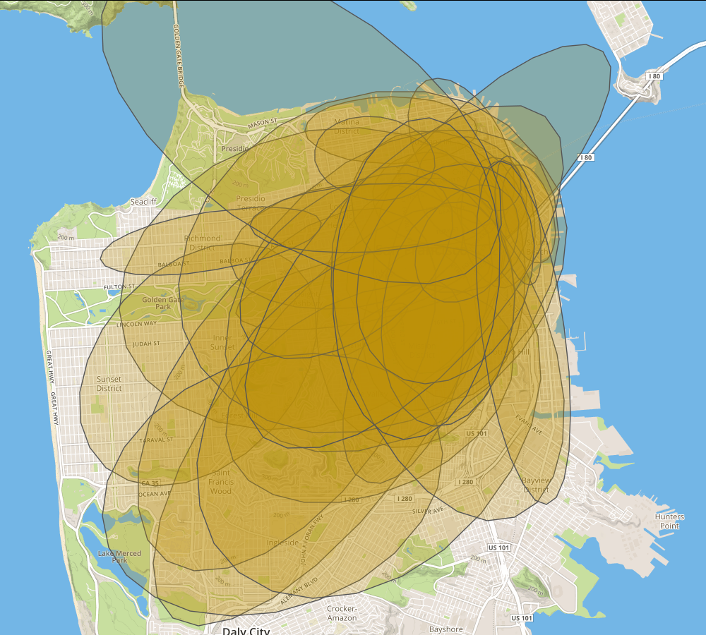
(b) Our method

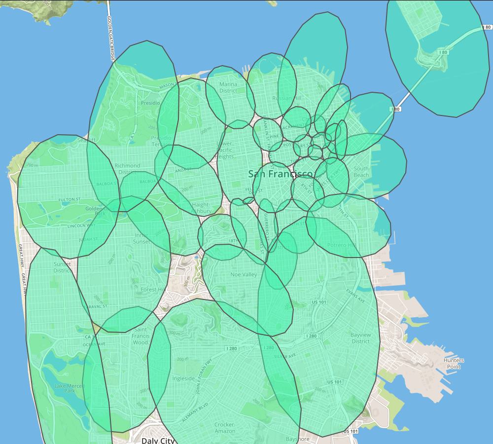
(c) Livehoods

Figure 8: In San Francisco, the middle panel shows the regions we obtained with our probabilistic model. On the left, Hoodsquare regions are extracted from their website and transformed into Gaussians. On the right is the same picture for Livehoods. All methods show that the city activity occurs mainly downtown but it also highlights differences between approaches. For instance, although Livehoods exhibits some overlap, it is only due to the Gaussian conversion whereas we do not restrain venues to serve a single function in a single region by construction, but only let that happens if the data support it.

7 Related Work

Urban Computing is an active area of research, partially due to the increasing volume of digital data related to human activity and the potential to use such data to improve life in cities. Below, we discuss related works that either address a similar task (finding geographical structure in city activity) or use a similar approach to ours to address different tasks (Section 7.1). To the best of our knowledge, we are the first to employ a fully probabilistic approach to this task – and thus discuss further the concept of sparse modeling (Section 7.2). Moreover, we discuss briefly other tasks pertaining to Urban Computing that are more loosely related to our work (Section 7.3).

7.1 Finding structure in urban activity from digital traces

Finding cohesive geographical regions within cities has been attempted using a variety of data sources, such as cellphone activity [8], geotagged tweets [9], social interactions [10], types of buildings [11], or public transport and taxi trajectories [12, 13].

In that context, Location Based Social Networks (LBSNs) have also proven a rich source of data and utilized by recent works. For instance, [4] collects checkins and build a $m$-nearest spatial neighbors graph of venues, with edges weighted by the cosine similarity of both venue’s user distribution. The regions are the spectral clusters of this graph. Using similar data, [5] describes venues by category, peak time activity and a binary touristic indicator. Venues are clustered in hotspots along all these dimensions by the OPTICS algorithm. The city is divided into a grid, with cells described by their hotspot density for each feature. Finally, similar cells are iteratively clustered into regions. Like us, [14] considers venues to be essential in defining regions. The city is divided into a grid of cells with the goal of assigning each cell a category label in a way that is as specific as possible while being locally homogeneous. This is done through a bottom-up clustering which greedily merge neighboring cells to improve a cost function formalizing this trade off.

While these results are evaluated with user interviews and built upon well known algorithmic techniques, they rely on ad-hoc modeling decisions (such graph construction and grid granularity) that do not derive directly from the data, and thus leave us at a loss when we are asked to support the statistical significance of the obtained results. Furthermore, because the clustering is not guided simultaneously by all the available data features, such as time and aspects other than venue category, important information might be going amiss in those approaches.

On the other hand, there are works that take a probabilistic approach, although their aim is different than ours. For instance, [15] assigns venues to a grid and runs Latent Dirichlet Allocation (LDA) on their categories. However it does not output explicit regions, and the grid is coarse approximation for using spatial information. Instead, [16] fixes a number $K$ of localized topics to be discovered, as well as a set of $N$ Gaussian spatial regions. Each region has a topic distribution and each topic is a multinomial distribution over all possible Flickr photos tags. Relaxing several assumptions, notably the Gaussian shape, [17] extends Hierachical Dirichlet Process to spatial data, giving rise to an almost fully non-parametric model (as the number of regions still needs to be set manually). One extension of such methods is to take users features into account, in order to provide recommendations [18]. While such methods bear similarity with ours, the domain of application presented by their authors forbids direct comparisons.

Closer to the task of finding regions, [19] performs LDA on checkins in New York. The five resulting topics are called urban activities, and venues are clustered by their topic proportion across time. Contrary to us, this clustering does not produce clearly defined regions as it is done as a post processing step. Indeed, their LDA model does not incorporate a spatial dimension. Moving from checkins to a dataset of 8 millions Flickr geotagged photos, [20] probabilistically assigns tags to one of the three levels of a spatial hierarchy, where each node is associated with a multinomial distribution over tags. This allow to find the most descriptive tags for a given regions and thus characterize it. Like in our work, a measure of similarity between regions is defined.

7.2 Sparse topic model

We now present related applications of the Sparse additive generative model on spatial data. The original SAGE paper [3] evaluates its model effectiveness on the task of predicting the localization of twitter users by learning not only topics about words but also about metadata (i.e. in which region was the tweet written) and shows good accuracy. Later, a simplified version of it was used to find regions which exhibit geolocated idioms [21]. It is possible to better model user location by building a hierarchy of regions [22]. Even though the sparsity of model is well suited to the sparsity of textual data, note that methods which do not use topic modelling give competitive results in terms of accuracy [23, 24].

Another task hindered by data sparsity and which benefits from modeling user preferences is spatial item recommendation. The interested reader will find many examples exploiting LBSN in a recent survey [25], but here we give a taste of two approaches inspired by SAGE. In both cases, topics are distributions over words and venues. Each user is endowed with her own topic, and so to are each region. [26] uses SAGE to model user topics as a variation from the overall global distribution. To improve out of town recommendation, [27] assigns regions both local and tourist topics. Learning such high number of parameters is made possible by combining SAGE and a hierarchical model called spatial pyramid.

7.3 Other urban computing problems

After finding regions in a city, a natural task is to compare them, within or across cities. One might also look at different granularity to perform such urban comparisons, whether points of interest or cities as a whole. Finally, one might focus on users and model their preferences through mobility data.

Comparing regions

We saw that one way to compare regions is to assign them descriptive tags [20]. Others have looked at a more information retrieval approach [28], while in [6], authors collect data from Foursquare and Flickr to associate venues with a features vector summarizing their time activity, their surroundings, their category and their popularity. They then define the similarity between two regions as the Earth Mover Distance between the two sets of venues feature vectors they contain. Finally they devise a pruning and clustering strategy to perform efficient search.

Finding points of interest

Regions are only one subdivision of the city, another one are points of interest, which are locations where the user activity show some specificities. Geotagged photos can be mined to extract the semantics of such locations [29, 30, 31, 32, 33]. As a representative example, [34] compares various spatial methods to discover small areas in San Francisco where one photo tag appears in burst. GPS trajectories provide useful information as well [35, 36, 37]. For instance, [38] extracts stay points from car GPS data and assess their significance by how many visitors go there, how far they traveled to reach them and how long they stay.

Comparing cities

This has been done by comparing the spatial distribution of human hotspots using call data [39], the call data profile themselves [40], the distribution of venues category at various scales [41], or by building a network of city from urban residents mobility flow and computing centrality measures [42].

Clustering users

With venues, users are the other side of the coin of what defines a region in a city, and some works have mine their activities to extract meaningful groups. For instance, [43] clusters users by the similarity of their venues category transition probability matrix. Another approach is to consider users as document, checkins as word and apply LDA, thus revealing cohesive communities [44] and describing people lifestyle [45].

One can find other applications of Urban Computing in related literature surveys [1, 46].

8 Conclusions

In this work, we made use of a probabilistic model to reveal how venues are distributed in cities in terms of several features. As most habitants of a city do not visit most of the available venues, we cope with the induced sparsity by adapting the sparse modeling approach of [3] to data at hand. Fitting our model to a large dataset of more than 11 million checkins in 40 cities around the world, we show the insights provided by such an unsupervised approach.

First, using the extracted model instances, we calculated the probability distribution of a single feature conditioned on the location in the city. This enabled us to construct a heatmap of that feature to highlight what feature values are most likely and distinctive at different locations within a city.

Secondly, we described a principled approach to quantify the importance of different features within the trained models. Whereas all features contribute, we discovered that the most defining feature for the components uncovered by the model is the visitors of venues. This finding suggests that further analysis of user behavior is a promising direction for extracting additional insights.

Third, after focusing on the various regions of a single city, we used the extracted model instances to find the most two similar regions between two cities, a task which was previously attempted with a more heuristic approach [6]. This time we also benefit of the solid theoretical grounds of probabilistic models to define principled measures of similarity and we describe a procedure to greedily find two regions which maximize such measures.

Finally, we compare our approach with previous approaches that provide similar output and show that our regions are both more consistent with the data (in terms of predictive performance) and have more sharply defined characteristics, meaning they are easier to distinguish from one another.

A review of recent related works in the Urban Computing field suggests that whereas the area is active and that understanding urban activities is a worthy endeavour which benefits from geotagged data, it can be pushed further by the use of probabilistic models, as such models come with great interpretative power.

Looking beyond this paper, there are further directions in which we can improve our discovery process, providing additional interpretation along the way:

• The first direction is to use a different evaluation process, one that would involve more closely users, since we show they are the main actor of the regions we discover. For instance, this could take the form of interviews. The purpose of this would be to identify and correct, if any, significant biases that are embodied in particular datasets (Foursquare activity, in our case).

• The model itself could also be extended, for instance by incorporating hierarchies of regions. This would both provide more structure to our results and allow us to apply our method to larger geographical area while keeping sparsity and runtime under control. Hierarchy is a well studied concept in both spatial data mining and topic modelling [47] and thus we are confident this would be a feasible improvement. Another direction would be to incorporate additional features into the model (e.g., continuous features)

• Just as natural landscapes change with time, whether because of the day/night cycle or the passing of seasons, so do cities. It is not far fetched to imagine than coastal areas of Barcelona or San Francisco witness different patterns of activities in the winter than in the summer. Again following the time evolution of topics has been addressed in different settings [48].

• There is the opportunity to use the automatically extracted models to build advanced systems. One direction would be to involve users in a discovery-and-feedback process, where users would indicate regions they appreciate in their hometown and the system would help them plan a trip in a new city based on model instances trained for the two cities.

Emre Çelikten is a graduate student at Aalto University. Previously he has worked as a software engineer focusing on scalable web back-end development. He received his Bachelor’s degree from the Computer Engineering department of İzmir Institute of Technology. He is currently serving as research assistant at Aalto University. His research interests include machine learning and mining social media data.

Géraud Le Falher is a PhD student at Inria Lille. He received his Master of Engineering from École Centrale de Nantes, France and his Master’s degree from the Computer Science department of Aalto University. His research interests include mining urban data and learning with graph data, especially in the context of signed graphs.

Michael Mathioudakis is a postdoctoral researcher at the Helsinki Institute for Information Technology HIIT and Aalto University. He received his PhD from the Department of Computer Science at the University of Toronto in 2013. His research interests focus mostly on the analysis of user-generated content on the Web, including the analysis of information diets on the Web, urban informatics, and trend detection on social media.

References

- [1] Y. Zheng, L. Capra, O. Wolfson, and H. Yang, “Urban Computing: Concepts, Methodologies, and Applications,” ACM Transaction on Intelligent Systems and Technology, vol. 5, no. 3, pp. 38:1–38:55, 2014.
- [2] “World Urbanization Prospects, the 2014 Revision: Highlights,” United Nations, Department of Economic and Social Affairs, Population Division, New-York, Tech. Rep., 2014.
- [3] J. Eisenstein, A. Ahmed, and E. P. Xing, “Sparse Additive Generative Models of Text,” in Proceedings of the International Conference on Machine Learning (ICML), Seattle, WA, 2011, pp. 1041–1048.
- [4] J. Cranshaw, J. I. Hong, and N. Sadeh, “The livehoods project: Utilizing social media to understand the dynamics of a city,” in ICWSM, 2012, pp. 58–65.
- [5] A. X. Zhang, A. Noulas, S. Scellato, and C. Mascolo, “Hoodsquare: Modeling and recommending neighborhoods in location-based social networks,” in ASE/IEEE SocialCom, 2013, pp. 69–74.
- [6] G. Le Falher, Gionis Aristides, and M. Mathioudakis, “Where Is the Soho of Rome? Measures and Algorithms for Finding Similar Neighborhoods in Cities,” in International AAAI Conference on Web and Social Media, Oxford, 2015.
- [7] S. C. Deerwester, S. T. Dumais, T. K. Landauer, G. W. Furnas, and R. A. Harshman, “Indexing by latent semantic analysis,” JAsIs, vol. 41, no. 6, pp. 391–407, 1990.
- [8] J. L. Toole, M. Ulm, M. C. González, and D. Bauer, “Inferring Land Use from Mobile Phone Activity,” in Proceedings of the ACM SIGKDD International Workshop on Urban Computing, New York, NY, USA, 2012, pp. 1–8.
- [9] V. Frias-Martinez and E. Frias-Martinez, “Spectral clustering for sensing urban land use using Twitter activity,” Engineering Applications of Artificial Intelligence, vol. 35, pp. 237–245, 2014.
- [10] J. R. Hipp, R. W. Faris, and A. Boessen, “Measuring ‘neighborhood’: Constructing network neighborhoods,” Social Networks, vol. 34, no. 1, pp. 128–140, 2012.
- [11] Z. Cao, S. Wang, G. Forestier, A. Puissant, and C. F. Eick, “Analyzing the Composition of Cities Using Spatial Clustering,” in Proceedings of the 2nd ACM SIGKDD International Workshop on Urban Computing, New York, NY, USA, 2013, pp. 14:1–14:8.
- [12] N. J. Yuan, Y. Zheng, X. Xie, Y. Wang, K. Zheng, and H. Xiong, “Discovering Urban Functional Zones Using Latent Activity Trajectories,” Knowledge and Data Engineering, IEEE Transactions on, vol. 27, no. 3, pp. 712–725, 2015.
- [13] Jichang Zhao, Ruiwen Li, X. Liang, and K. Xu, “Segmentation and evolution of urban areas in beijing: A view from mobility data of massive individuals,” in Proceedings of the 12th International Conference on Service Systems and Service Management (ICSSSM), 2015.
- [14] C. Vaca, D. Quercia, F. Bonchi, and P. Fraternali, “Taxonomy-Based Discovery and Annotation of Functional Areas in the City,” in ICWSM, 2015, pp. 445–453.
- [15] J. Cranshaw and T. Yano, “Seeing a home away from the home: Distilling proto-neighborhoods from incidental data with Latent Topic Modeling,” in NIPS’10 Workshop of Computational Social Science and the Wisdom of the Crowds, 2010.
- [16] Z. Yin, L. Cao, J. Han, C. Zhai, and T. Huang, “Geographical Topic Discovery and Comparison,” in Proceedings of the 20th International Conference on World Wide Web, 2011, pp. 247–256.
- [17] C. C. Kling, J. Kunegis, S. Sizov, and S. Staab, “Detecting non-gaussian geographical topics in tagged photo collections,” in Proceedings of the 7th ACM international conference on Web search and data mining (WSDM), 2014, pp. 603–612.
- [18] T. Kurashima, T. Iwata, T. Hoshide, N. Takaya, and K. Fujimura, “Geo Topic Model: Joint Modeling of User’s Activity Area and Interests for Location Recommendation,” in Proceedings of the Sixth ACM International Conference on Web Search and Data Mining, 2013, pp. 375–384.
- [19] F. Kling and A. Pozdnoukhov, “When a city tells a story: urban topic analysis,” in 20th International Conference on Advances in Geographic Information Systems - SIGSPATIAL ’12, 2012, pp. 482–485.
- [20] M. Kafsi, H. Cramer, B. Thomee, and D. A. Shamma, “Describing and Understanding Neighborhood Characteristics through Online Social Media,” in WWW, Florence, 2015, pp. 549—-559.
- [21] J. Eisenstein, “Written dialect variation in online social media,” in Handbook of Dialectology, 2015.
- [22] A. Ahmed, L. Hong, and A. J. Smola, “Hierarchical Geographical Modeling of User Locations from Social Media Posts,” in Proceedings of the 22nd International Conference on World Wide Web, Republic and Canton of Geneva, Switzerland, 2013, pp. 25–36.
- [23] R. Priedhorsky, A. Culotta, and S. Y. Del Valle, “Inferring the Origin Locations of Tweets with Quantitative Confidence,” in Proceedings of the 17th ACM Conference on Computer Supported Cooperative Work & Social Computing, New York, NY, USA, 2014, pp. 1523–1536.
- [24] D. Flatow, M. Naaman, K. E. Xie, Y. Volkovich, and Y. Kanza, “On the Accuracy of Hyper-local Geotagging of Social Media Content,” in Proceedings of the Eighth ACM International Conference on Web Search and Data Mining, New York, NY, USA, 2015, pp. 127–136.
- [25] J. Bao, Y. Zheng, D. Wilkie, and M. Mokbel, “Recommendations in location-based social networks: a survey,” GeoInformatica, vol. 19, no. 3, pp. 525–565, 2015.
- [26] B. Hu and M. Ester, “Spatial Topic Modeling in Online Social Media for Location Recommendation,” in Proceedings of the 7th ACM Conference on Recommender Systems, New York, NY, USA, 2013, pp. 25–32.
- [27] W. Wang, H. Yin, L. Chen, Y. Sun, S. Sadiq, and X. Zhou, “Geo-SAGE: A Geographical Sparse Additive Generative Model for Spatial Item Recommendation,” in Proceedings of the 21th ACM SIGKDD International Conference on Knowledge Discovery and Data Mining (KDD), New York, New York, USA, 2015, pp. 1255–1264.
- [28] C. Sheng, Y. Zheng, W. Hsu, M. Lee, and X. Xie, “Answering Top-k Similar Region Queries,” in Database Systems for Advanced Applications, 2010, vol. 5981, pp. 186–201.
- [29] D.-P. Deng, T.-R. Chuang, and R. Lemmens, “Conceptualization of place via spatial clustering and co-occurrence analysis,” in Proceedings of the 2009 International Workshop on Location Based Social Networks, New York, New York, USA, 2009, pp. 49–56.
- [30] M. Shirai, M. Hirota, S. Yokoyama, N. Fukuta, and H. Ishikawa, “Discovering Multiple HotSpots Using Geo-tagged Photographs,” in Proceedings of the 20th International Conference on Advances in Geographic Information Systems, 2012, pp. 490–493.
- [31] M. Ruocco and H. Ramampiaro, “Exploratory Analysis on Heterogeneous Tag-point Patterns for Ranking and Extracting Hot-spot Related Tags,” in Proceedings of the 5th ACM SIGSPATIAL International Workshop on Location Based Social Networks, 2012, pp. 16–23.
- [32] R. Feick and C. Robertson, “A multi-scale approach to exploring urban places in geotagged photographs,” Computers, Environment and Urban Systems, 2014.
- [33] Y. Hu, S. Gao, K. Janowicz, B. Yu, W. Li, and S. Prasad, “Extracting and understanding urban areas of interest using geotagged photos,” Computers, Environment and Urban Systems, vol. 54, pp. 240–254, 2015.
- [34] T. Rattenbury and M. Naaman, “Methods for extracting place semantics from Flickr tags,” ACM Transactions on the Web, vol. 3, no. 1, pp. 1–30, 2009.
- [35] M. R. Uddin, C. Ravishankar, and V. J. Tsotras, “Finding Regions of Interest from Trajectory Data,” in 2011 IEEE 12th International Conference on Mobile Data Management, vol. 1, 2011, pp. 39–48.
- [36] C. Zhang, J. Han, L. Shou, J. Lu, and T. L. Porta, “Splitter: Mining Fine-Grained Sequential Patterns in Semantic Trajectories,” Proceedings of the VLDB Endowment, vol. 7, no. 9, pp. 769–780, 2014.
- [37] C. Parent, S. Spaccapietra, C. Renso, G. Andrienko, N. Andrienko, V. Bogorny, M. L. Damiani, A. Gkoulalas-Divanis, J. Macedo, N. Pelekis, Y. Theodoridis, and Z. Yan, “Semantic Trajectories Modeling and Analysis,” ACM Comput. Surv., vol. 45, no. 4, pp. 42:1—-42:32, 2013.
- [38] X. Cao, G. Cong, and C. S. Jensen, “Mining significant semantic locations from GPS data,” Proceedings of the VLDB Endowment, vol. 3, no. 1-2, pp. 1009–1020, 2010.
- [39] T. Louail, M. Lenormand, O. G. Cantu Ros, M. Picornell, R. Herranz, E. Frias-Martinez, J. J. Ramasco, and M. Barthelemy, “From mobile phone data to the spatial structure of cities,” Scientific Reports, vol. 4, 2014.
- [40] S. Grauwin, S. Sobolevsky, S. Moritz, I. Gódor, and C. Ratti, “Towards a comparative science of cities: Using mobile traffic records in new york, london, and hong kong,” in Computational Approaches for Urban Environments, 2015, vol. 13, pp. 363–387.
- [41] D. Preoţctiuc-Pietro, J. Cranshaw, and T. Yano, “Exploring Venue-based City-to-city Similarity Measures,” in Proceedings of the 2nd ACM SIGKDD International Workshop on Urban Computing, New York, NY, USA, 2013, pp. 16:1–16:4.
- [42] M. Lenormand, B. Gonçalves, A. Tugores, and J. J. Ramasco, “Human diffusion and city influence,” Journal of The Royal Society Interface, vol. 12, no. 109, 2015.
- [43] D. Preoţiuc-Pietro and T. Cohn, “Mining user behaviours: A study of check-in patterns in location based social networks,” in Proceedings of the 5th Annual ACM Web Science Conference, New York, NY, USA, 2013, pp. 306–315.
- [44] K. Joseph, C. H. Tan, and K. M. Carley, “Beyond ‘Local’, ‘Categories’ and ‘Friends’: Clustering Foursquare Users with Latent ‘Topics’,” in Proceedings of the 2012 ACM Conference on Ubiquitous Computing, New York, NY, USA, 2012, pp. 919–926.
- [45] N. J. Yuan, F. Zhang, D. Lian, K. Zheng, S. Yu, and X. Xie, “We Know How You Live: Exploring the Spectrum of Urban Lifestyles,” in Proceedings of the First ACM Conference on Online Social Networks, New York, NY, USA, 2013, pp. 3–14.
- [46] D. Tasse and J. Hong, “Using Social Media Data to Understand Cities,” in Proceedings of NSF Workshop on Big Data and Urban Informatics, 2014.
- [47] D. M. Blei, T. L. Griffiths, and M. I. Jordan, “The nested chinese restaurant process and bayesian nonparametric inference of topic hierarchies,” J. ACM, vol. 57, no. 2, pp. 7:1–7:30, 2010.
- [48] D. M. Blei and J. D. Lafferty, “Dynamic topic models,” in Proceedings of the 23rd International Conference on Machine Learning, 2006, pp. 113–120.