Constructing valid density matrices on an NMR quantum information processor via maximum likelihood estimation

Abstract

Estimation of quantum states is one of the most important steps in any quantum information processing experiment. A naive reconstruction of the density matrix from experimental measurements can often give density matrices which are not positive, and hence not physically acceptable. How do we ensure that at all stages of reconstruction, we keep the density matrix positive and normalized? Recently a method has been suggested based on maximum likelihood estimation, wherein the density matrix is guaranteed to be positive definite. We experimentally implement this protocol and demonstrate its utility on an NMR quantum information processor. We discuss several examples where we undertake such an estimation and compare it with the standard method of state estimation.

I Introduction

How do we assign a state to a physical system? Classically the answer is very simple: we determine the phase space point corresponding to the configuration of the system. This can be achieved by measuring the relevant system parameters in an non-invasive manner. However, for quantum systems non-invasive measurements are not possible, and therefore we typically need an ensemble of identically prepared systems to perform state estimation. Since the quantum state cannot be known from a single measurement and the no-cloning theorem precludes the possibility of making several copies of the state and using them to make different measurements on the same state, quantum state estimation is intrinsically a statistical process Massar and Popescu (1995); Derka et al. (1998). Furthermore, since ensembles are always finite, there is always some ambiguity associated with the estimated state. For a given physical situation, we may even have two different candidate states! Can these uncertainties and ambiguities be such that sometimes we end up estimating the state to be a non-state? Such estimates should be not allowed and any error or ambiguity in state estimation should be within the space of positive normalized density operators.

Complete estimation of a quantum state from a set of measurements on a finite ensemble has been a hot topic of research in quantum information and experimental quantum computing and several schemes have been proposed and implemented for quantum state estimation Paris and Rehacek (2004); Cramer et al. (2010); Rehacek et al. (2015). Standard methods of reconstructing an unknown state from a set of measurements rely on quantum state tomography (QST) protocols Helstrom (1976); Smithey et al. (1993); Thew et al. (2002). The QST method is based on averaging a specialized function over the experimental data obtained using a quorum of observables, sufficient to reconstruct the state. However, the QST averaging procedure leads to fluctuations which could result in significant statistical errors as well as an unphysical density matrix i.e., some eigenvalues could turn out to be negative. A scheme that redresses this issue of reconstructed density matrices that are unphysical, is the maximum-likelihood estimation (MLE) scheme, which obtains a positive definite estimate for the density matrix by optimizing a likelihood functional that links experimental data to the estimated density matrix Banaszek et al. (1999); Hradil (1997); Blume-Kohout (2010); Baumgratz et al. (2013). The MLE scheme begins with a guess quantum state and improves the estimate based on the measurements made; the more the number of measurements, the better is the state estimate. A tomographic protocol for two qubits was recently constructed based on the measurement of 16 generalized Pauli operators which is maximally robust against errors Miranowicz et al. (2014). A refined iterative maximum-likelihood algorithm was also proposed to reconstruct a quantum state and applied to the tomography of optical states and entangled spin states of trapped ions Rehacek et al. (2007). Other quantum state estimation algorithms include Bayesian mean estimation Huszar and Houlsby (2012), least-squares inversion Opatrny et al. (1997), numerical strategies for state estimation Kaznady and James (2009) and linear regression estimation Qi et al. (2013).

In this work we demonstrate the utility of the MLE scheme to estimate quantum states on an NMR quantum information processor. We experimentally prepare separable and entangled states of two and three qubits, and reconstruct the density matrices using both the MLE scheme as well as QST. Further, we define an entanglement parameter to quantify multiqubit entanglement and estimate entanglement using both the QST and the MLE schemes. We show that while the QST method overestimates the residual state entanglement at a given time, the MLE method is able to give us a correct estimate of the amount of entanglement present in the state. This is the first demonstration of the advantages of using MLE for state estimation over QST for NMR quantum information processing.

The paper is organized as follows: Section II contains a concise theoretical description of how to use QST and MLE to estimate a quantum state. Section III describes the NMR implementation of the MLE method in estimating quantum states of two and three qubits and a comparison of results obtained using QST. Section III.1 contains a discussion of using MLE to reconstruct an entangled state on an NMR quantum information processor. Section IV contains some concluding remarks.

II Density matrix reconstruction

II.1 Quantum state tomography

Quantum state tomography (QST) aims to completely reconstruct an unknown state via a set of measurements on an ensemble of identically prepared states. Any density matrix $\rho$ of $n$ qubits in a $2^{n}$-dimensional Hilbert space can be uniquely determined using $4^{n}-1$ independent measurements and the state of the system as described by its density operator $\rho$ can be reconstructed by performing a set of projective measurements on multiple copies of the state Chen et al. (2013); Vandersypen and Chuang (2005). Determining all the elements of $\rho$ would involve making repeated measurements of the same state in different measurement bases, until all the elements of $\rho$ are determined Smithey et al. (1993); Thew et al. (2002); James et al. (2001).

In NMR we cannot perform projective measurements and instead measure the expectation values of certain fixed operators over the entire ensemble. Therefore, we rotate the state via different unitary transformations before performing the measurement to collect information about different elements of the density matrix Vandersypen and Chuang (2005). The standard tomographic protocol for NMR uses the Pauli basis to expand an $n$ qubit $\rho$,

$$\rho=\sum_{i=0}^{3}\sum_{j=0}^{3}...\sum_{k=0}^{3}c_{ij...k}\sigma_{i}\otimes\sigma_{j}\otimes....\sigma_{k}$$ (1)

where $c_{00...0}=1$ and $\sigma_{0}$ denotes the $2\times 2$ identity matrix while $\sigma_{1}$, $\sigma_{2}$ and $\sigma_{3}$ are standard Pauli matrices. The measurement of expectation values allowed in an NMR experiment combined with unitary rotations leads to the determination of the coefficients $c_{ij..k}$.

In an NMR experiment, we measure the signal induced in the detection coils while the nuclear spins precess freely in a strong applied magnetic field. This signal is called the free induction decay (FID) and is proportional to the time rate of change of magnetic flux. This time-domain signal can be expressed in terms of the expectation values of the transverse magnetization Leskowitz and Mueller (2004):

$$S(t)\propto\mbox{Tr}\left\{\rho(t)\sum_{k}(I_{kx}-iI_{ky})\right\}$$ (2)

where $I_{kx}=\frac{1}{2^{n}}(I_{1}\otimes\cdots\sigma_{kx}\cdots\otimes I_{n})$ and $\frac{1}{2^{n}}(I_{ky}=I_{1}\otimes\cdots\sigma_{ky}\cdots\otimes I_{n})$ are the Cartesian angular momentum operators (subset of the product operators) for the spin $k$ and $\rho(t)$ is the density operator at time $t$. This signal is then Fourier transformed to extract information about expectation values of different operators. In NMR, products of a set of the identity operator and the Pauli spin operators, form the quorum of observables for QST Chuang et al. (1998); Lee (2002); Long et al. (2001). While the measured expectation values remain the same, unitary operators in terms of rf pulses are applied before measurement to effectively measure the expectation values of different operators.

For a system of two qubits, the density matrix can be expanded in terms of product operators $I_{1}\otimes I_{2}\dots\sigma_{1z}\otimes\sigma_{2z}$, as follows:

$$\rho = \frac{1}{4}I_{1}\otimes I_{2}+\langle\sigma_{1x}\otimes I_{2}\rangle\sigma_{1x}\otimes I_{2}+\dots$$ (3)

$$+\langle\sigma_{1z}\otimes\sigma_{2y}\rangle\sigma_{1z}\otimes\sigma_{2y}+\langle\sigma_{1z}\otimes\sigma_{2z}\rangle\sigma_{1z}\otimes\sigma_{2z}$$

and $\langle\sigma_{1x}\otimes I_{2}\rangle$,$\dots$, $\langle\sigma_{1z}\otimes\sigma_{2z}\rangle$ can be measured by different NMR experiments. The FID is collected after the application of four unitary operators denoted by $\mathbf{I}\mathbf{I}$, $\mathbf{I}X$, $\mathbf{I}Y$, and $XX$, where $\mathbf{II}$ corresponds to “no operation” on both spins, $\mathbf{I}X(Y)$ corresponds to a “no operation” on the first spin and a $90^{\circ}$ rf pulse of phase $X(Y)$ on the second spin, and $XX$ corresponds to a $90^{\circ}$ rf pulse of phase $X$ on both spins. Fourier transform after this FID collection leads to the extraction of desired expectation values.

As an example for a two-qubit system, we tried creating the the quantum state $\frac{1}{\sqrt{2}}(|00\rangle+|01\rangle)$ and reconstructed it using standard QST. The reconstructed density matrix $\rho_{\mbox{QST}}$ turned out to be

$${\bf\rho_{\mbox{QST}}}=\left(\begin{array}[]{cccc}0.4938&0.5003+i0.0014&-0.0221-i0.0551&-0.0102+i0.1282\\ 0.5003-i0.0014&0.5062&0.0279-i0.1309&0.0168+i0.0695\\ -0.0221+i0.0551&0.0279+i0.1309&-0.0482&0.0030-i0.0378\\ -0.0102-i0.1282&0.0168-i0.0695&0.0030+i0.0378&0.0482\end{array}\right)$$ (4)

The above density matrix $\rho_{\mbox{QST}}$ reconstructed using the QST protocol is normalized and Hermitian and its eigenvalues are {1.0360, 0.0926, -0.0179, -0.1106}. As is clear from the last two eigenvalues, the reconstructed density matrix is not positive, and furthermore, $\mbox{Tr}(\rho^{2}_{\mbox{QST}})=1.0944$. Density matrices that represent physical quantum states must have the property of positive definiteness which, in conjunction with the properties of normalization and Hermiticity, implies that all the eigenvalues must lie in the interval [0,1] and sum to 1 i.e. $0\leq\mbox{Tr}(\rho^{2})\leq 1$. Clearly, the density matrix reconstructed above by standard QST violates this condition. Due to its negative eigenvalues it has as a strange feature that $\mbox{Tr}(\rho^{2})>\mbox{Tr}(\rho)$. The obvious reasons for this problem are experimental inaccuracies, which implies that the actual magnetization values recorded in an NMR experiment differ from those that can be obtained from the Eqn. (3). However, in a correct estimation scheme the experimental inaccuracies should lead to an error in the state estimation by giving a state which is close to the actual state with some confidence level and should not give a non-state! An ad hoc way to circumvent this problem is to add a multiple of identity to this density matrix so that the eigenvalues are positive. However, this kind of addition is completely ad-hoc and leads to non-optimal estimates and one should be able to do better. We turn to this issue in the next section via the maximum likelihood estimation method.

II.2 Maximum likelihood estimation

The example in the previous section illustrates that most density matrices tomographed using standard QST may not correspond to a physical quantum state. To address this problem, the maximum likelihood estimation (MLE) method was developed to ensure that the reconstructed density matrix is always positive and normalized James et al. (2001). The MLE method estimates the entire quantum state, by finding the parameters that are most likely to match the experimentally generated data and maximizing a specific target function; a priori knowledge of the density matrix can also be incorporated into the method. The main advantage of the method is that at every stage of the estimation process the density matrix is positive and normalized and therefore represents a valid physical situation.

For a system of two qubits, the density matrix can be written in a compact form following Eqn. (1):

$$\rho=\sum_{j=0}^{3}\sum_{k=0}^{3}n_{jk}\sigma_{j}\otimes\sigma_{k}$$ (5)

where $n_{jk}$ are real coefficients determining the state.

A physical density matrix $\rho$ has to be Hermitian, positive and must have trace equal to unity. Such a density matrix can be written in terms of a lower triangular matrix $T$ James et al. (2001)

$$\rho=T^{{\dagger}}T\quad\mbox{Tr}(T^{{\dagger}}T)=1$$ (6)

For the two-qubit system the lower triangular matrix $T$ from which we obtain $\rho$ has 15 independent real parameters (one parameter from the 16 is eliminated due to the trace condition), and can be written in

$$T=\left(\begin{array}[]{cccc}t_{1}&0&0&0\\ t_{5}+it_{6}&t_{2}&0&0\\ t_{11}+it_{12}&t_{7}+it_{8}&t_{3}&0\\ t_{15}+it_{16}&t_{13}+it_{14}&t_{9}+it_{10}&t_{4}\end{array}\right)$$ (7)

Given a valid density matrix as described in James et al. (2001), it is possible to invert Eqn. (6) to obtain the matrix $T$

$$T=\left(\begin{array}[]{cccc}\sqrt{\frac{\Delta}{\mathcal{M}_{11}^{(1)}}}&0&0&0\\ {\frac{\mathcal{M}_{12}^{(1)}}{\sqrt{\mathcal{M}_{11}^{(}1)\mathcal{M}_{11,22}^{(2)}}}}&\sqrt{\frac{\mathcal{M}_{11}^{(1)}}{\mathcal{M}_{11,22}^{(2)}}}&0&0\\ {\frac{\mathcal{M}_{12,23}^{(2)}}{\sqrt{\rho_{44}}\sqrt{\mathcal{M}_{11,23}^{(2)}}}}&\frac{\mathcal{M}_{11,22}^{(2)}}{\sqrt{\rho_{44}}\sqrt{\mathcal{M}_{11,22}^{(2)}}}&\sqrt{\frac{\mathcal{M}_{11,22}^{(2)}}{\rho_{44}}}&0\\ \frac{\rho_{41}}{\sqrt{\rho_{44}}}&\frac{\rho_{42}}{\sqrt{\rho_{44}}}&\frac{\rho_{43}}{\sqrt{\rho_{44}}}&\sqrt{\rho_{44}}\end{array}\right)$$ (8)

where $\Delta=\mbox{Det}(\rho)$, $\mathcal{M}_{ij}^{(1)}$ is the first minor of $\rho$ (the determinant of the $3\times 3$ matrix formed by deleting the $i$th and $j$th columns of the $\rho$ matrix), $\mathcal{M}_{ij,kl}^{(2)}$ is the second minor of $\rho$ (the determinant of the $2\times 2$ matrix formed by deleting the $i$th and $k$th rows and $j$th and $l$th columns of the $\rho$ matrix with $i\neq j$ and $k\neq l$).

From the experimental data we obtain a set of expectation values $n_{jk}=\langle\sigma_{j}\otimes\sigma_{k}\rangle=\mbox{Tr}((\sigma_{j}\otimes\sigma_{k})\rho)$. It is generally assumed that the experimental noise has a Gaussian probability distribution and the probability of obtaining a set of measurement results for the set of expectation values $\{n_{jk}\}$ is

$$P(n_{11},\cdots n_{33})=A\prod_{j=0,k=0}^{3,3}exp\left[-\frac{(n_{jk}-\bar{n}_{jk})^{2}}{2\sigma_{jk}^{2}}\right]$$ (9)

where $A$ is a normalization constant and $\sigma_{jk}$ is the standard deviation of the measured variable $n_{jk}$ (approximately given by $\sqrt{\bar{n}_{jk}}$).

The first step in implementing the MLE is the generation of an initial physically valid density matrix. For instance, for a system of two qubits this matrix $\rho(t_{1},t_{2},\dots,t_{16})$ is a function of 16 real variables. The next step in the MLE method is to maximize the likelihood that the physical density matrix $\rho$ will give rise to the experimental data $\{n_{jk}\}$. Rather than finding the maximum value of the probability $P$, the optimization problem gets simplified by finding the maximum of its logarithm. Thus the optimization problem is reduced to finding the minimum of a “likelihood function”

$$\mathcal{L}(t_{1},\cdots t_{16})=\sum_{j=0,k=0}^{3,3}\frac{\left(n_{jk}(t_{1},\cdots t_{16})-\bar{n}_{jk}(t_{1},\cdots t_{16})\right)^{2}}{2\bar{\sigma}_{jk}^{2}}$$ (10)

For a system of two qubits, the optimum set of variables $\{t_{1}^{opt},t_{2}^{opt},\dots,t_{16}^{opt}\}$ which minimizes this likelihood function can be determined using numerical optimization techniques. We used the Matlab routine “lsqnonlin” MATLAB (2015) to find the minimum of the likelihood function. To execute this routine, one requires the initial estimation of the value of $t_{1},t_{2},\dots,t_{16}$. Since sixteen parameter optimization can be tricky, it is important to use a good initial guess for parameters. A reasonable way is to first estimate the state using the standard method, and obtain the values of $t_{i}$s using the Eqn. (8). Since the state may not be a physically allowed state the parameters obtained in this manner are not necessarily real. Thus for our initial guess we drop the imaginary part and use the real parts of each of $t_{i}$s as the initial estimate to go into the optimization routine. We used the same experimentally generated $\frac{1}{\sqrt{2}}(|00\rangle+|01\rangle)$ state (described in the example given in the earlier subsection), and re-computed the density matrix now using the MLE method, and obtained:

$${\bf\rho_{MLE}}=\left(\begin{array}[]{cccc}0.5013&0.4957+i0.0011&0.0004+i0.0067&0.0003+i0.0070\\ 0.4957-i0.0011&0.4958&0.0004+i0.0067&0.0003+i0.0070\\ 0.0004-i0.0067&0.0004-i0.0067&0.0014&0.0015+i0.0000\\ 0.0003-i0.0070&0.0003-i0.0070&0.0015-i0.0000&0.0017\end{array}\right)$$ (11)

The eigen values of this matrix are $\{0.9941,0.0030,0.0029,0.0000\}$ and are all positive and furthermore $\mbox{Tr}(\rho^{2}_{\mbox{MLE}})=0.9883$. While the density matrix reconstructed using QST was unphysical, the MLE reconstruction led to a valid density matrix.

III State estimation of two & three qubits

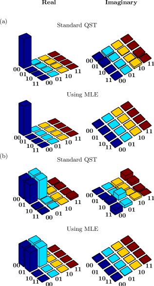
Figure 1: Real (left) and imaginary (right) parts of the experimental tomographs of the (a) $|00\rangle$ state, with a computed fidelity of 0.9833 using standard QST and a computed fidelity of 0.9889 using MLE for state estimation. (b) $\frac{1}{\sqrt{2}}(|00\rangle+|01\rangle)$ state, with a computed fidelity of 0.9952 using standard QST and a computed fidelity of 0.9939 using MLE for state estimation. The rows and columns are labeled in the computational basis ordered from $|00\rangle$ to $|11\rangle$.

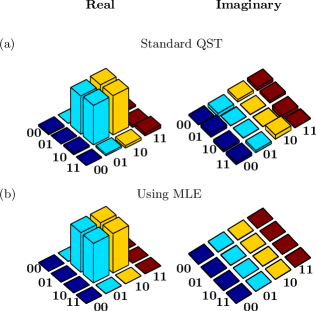
Figure 2: Real (left) and imaginary (right) parts of the experimental tomographs of the entangled state $\frac{1}{\sqrt{2}}(|01\rangle+|10\rangle)$ reconstructed (a) using standard QST and (b) using MLE. The fidelities computed using standard QST and using MLE for state estimation are 0.9879 and 0.9976 respectively. The rows and columns are labeled in the computational basis ordered from $|00\rangle$ to $|11\rangle$.

We performed state estimation of several different quantum states of two and three qubits, constructed on an NMR quantum information processor, using the MLE method. The results were compared every time with the results obtained by reconstruction using the standard QST protocol. The fidelity $F$ of all the states reconstructed in this section has been computed using the expression Weinstein et al. (2001)

$$F=\frac{Tr(\rho_{\rm theory}^{{\dagger}}\rho_{\rm expt})}{\sqrt{(}Tr(\rho_{\rm theory}^{{\dagger}}\rho_{\rm theory}))\sqrt{(}Tr(\rho_{\rm expt}^{{\dagger}}\rho_{\rm expt}))}$$ (12)

where $\rho_{\rm theory}$ and $\rho_{\rm expt}$ are the theoretically expected and experimentally reconstructed density matrices, respectively.

On a system of two qubits, we began by tomographing a pure state $|00\rangle$, as well as a superposition state $\frac{1}{\sqrt{2}}(|00\rangle+|01\rangle)$ (which can be written as a tensor product of the first qubit in the $|0\rangle$ state and the second qubit in a coherent superposition of the $|0\rangle$ and $|1\rangle$ states). The reconstructed density matrices using the MLE method and using the standard QST method are shown as bar tomographs in Figure 1, with the states labeled in the computational basis in the order $|00\rangle$ to $|11\rangle$. Using standard QST the reconstructed $|00\rangle$ state had negative eigenvalues: {0.9847, 0.0465, 0.0047, -0.0359} and state fidelity was computed to be 0.9833. Reconstructing the state using MLE, we obtained all positive eigenvalues: {0.9889, 0.0065, 0.0046, 0.0000}, while state fidelity was computed to be 0.9889. For the superposition state $\frac{1}{\sqrt{2}}(|00\rangle+|01\rangle)$, state reconstruction using standard QST led to some negative eigenvalues: {1.036, 0.0926, -0.0179, -0.1106} with a fidelity of 0.9952. Using MLE on the other hand, led to all positive eigenvalues: {0.9941, 0.0030, 0.0029, 0.0000} with a state fidelity of 0.9939. While state fidelities are nearly the same (or slightly better when calculated after MLE reconstruction of the density matrix), we find that by using the MLE method for state estimation, we always obtain a $\rho$ which is physically valid.

III.1 Estimation of entangled states

It has been previously noted James et al. (2001) that the standard QST protocol frequently leads to unphysical density matrices for entangled multiqubit states. Since entanglement has been posited to lie at the heart of quantum computational speedup, their construction and estimation is of prime importance. We used the MLE method to reconstruct two-qubit and three-qubit entangled states and evaluated the efficacy of this scheme to construct valid density matrices.

The state estimation of a two-qubit entangled Bell state $\frac{1}{\sqrt{2}}(|01\rangle+|10\rangle)$ is shown in Figure 2, using both QST and MLE for density matrix reconstruction. Using the QST [protocol for tomography, we obtain the eigenvalues: {0.9885, 0.0810, 0.0180, -0.0875} with the last eigenvalue being negative, and with a computed fidelity of 0.9879. Using MLE for state estimation leads to all positive eigenvalues: {0.9977, 0.0012, 0.006, 0.0005} with a computed state fidelity of 0.9976.

Recently, schemes to construct maximally entangled three-qubit states from a generic state have been implemented on an NMR quantum information processor Dogra et al. (2015); Das et al. (2015). We used these schemes to construct the maximally entangled $W$ state on a system of three qubits $|W\rangle=\frac{1}{\sqrt{3}}(i|001\rangle+|010\rangle+|100\rangle)$, and thereafter performed state estimation using both the standard QST and the MLE methods. The experimentally reconstructed tomographs are depicted in Figure 3, with the states being labeled in the computational basis ordered from $|000\rangle$ to $|111\rangle$. After QST tomography on this three-qubit state, we obtained the eigenvalues: {0.9399, 0.1037, 0.0780, 0.0544, -0.0018, -0.0419, -0.0612, -0.0713}, and a calculated state fidelity of 0.9759. After performing state estimation using the MLE method, the eigenvalues turned out to be all positive: {0.9191, 0.0361, 0.0267, 0.0075, 0.0064, 0.0024, 0.0015, 0.0000}, with a calculated state fidelity of 0.9968.

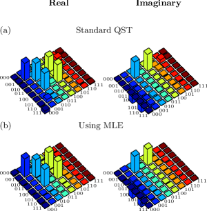
Figure 3: Real (left) and imaginary (right) parts of the experimental tomographs of the three-qubit maximally entangled state $|W\rangle=\frac{1}{\sqrt{3}}(i|001\rangle+|010\rangle+|100\rangle)$, reconstructed (a) using standard QST with a computed fidelity of 0.9833 and (b) using MLE with a computed fidelity of 0.9968. The rows and columns are labeled in the computational basis ordered from $|000\rangle$ to $|111\rangle$.

A topic of much research focus is the accurate measurement of the decay of multiqubit entanglement with time. To study this, we performed state estimation of the entangled two-qubit state $\frac{1}{\sqrt{2}}(|00\rangle+|11\rangle)$ using both QST and MLE protocols. The bar tomographs of the reconstructed density matrices at different times ($T=0,0.04,0.08,0.12,0.16$ sec) are shown in Figure 4.

The amount of entanglement that remains in the state after a certain time can be quantified by an entanglement parameter denoted by $\eta$ Singh et al. (2014). Since we are dealing with mixed bipartite states of two qubits, all entangled states will be negative under partial transpose (NPT). For such NPT states, a reasonable measure of entanglement is the minimum eigenvalue of the partially transposed density operator. For a given experimentally tomographed density operator $\rho$, we obtain $\rho^{PT}$ by taking a partial transpose with respect to one of the qubits. The entanglement parameter $\eta$ for the state $\rho$ in terms of the smallest eigenvalue $E^{\rho}_{\rm Min}$ of $\rho^{PT}$ is defined as Singh et al. (2014)

$$\eta=\left\{\begin{array}[]{ll}-E^{\rho}_{\rm Min}&{\rm if~{}}E^{\rho}_{\rm Min}<0\\ &\\ \phantom{-}0&{\rm if~{}}E^{\rho}_{\rm Min}>0\end{array}\right.$$ (13)

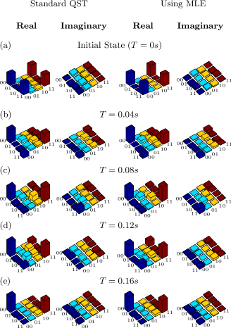
Figure 4: Real (left) and imaginary (right) parts of the experimental tomographs of the (a) $\frac{1}{\sqrt{2}}(|00\rangle+|11\rangle)$ state. (b)-(e) depict the state at $T=0.04,0.08,0.12,0.16s$, with the tomographs on the left and the right representing the state estimated using standard QST and using MLE, respectively. The rows and columns are labeled in the computational basis ordered from $|00\rangle$ to $|11\rangle$.

A plot of the entanglement parameter $\eta$ with time is depicted in Figure 5, for the two-qubit maximally entangled Bell state $\frac{1}{\sqrt{2}}(|00\rangle+|11\rangle)$, estimated using both standard QST and the MLE method. As can be seen from Figure 5, the QST method led to negative eigenvalues in the reconstructed (unphysical) density matrix and hence an overestimation of the entanglement parameter quantifying the residual entanglement in the state. The MLE method on the other hand, by virtue of its leading to a physical density matrix reconstruction every time, gives us a true measure of residual entanglement, and hence can be used to quantitatively study the decoherence of multiqubit entanglement.

Figure 5: Plot of the entanglement parameter $\eta$ with time, using standard QST and MLE for state reconstruction, computed for the $\frac{1}{\sqrt{2}}(|00\rangle+|11\rangle)$ state.

IV Conclusions

We have used the maximum likelihood estimation method for state estimation on an NMR quantum information processor, to circumvent the problem of unphysical density matrices that occur due to statistical errors while using the standard QST protocol. It has been previously shown that state reconstruction using QST, of entangled states and other fragile quantum states are particularly susceptible to errors, and can lead to unphysical density matrices for such states. We show that the experimental density matrices reconstructed for entangled states of two and three qubits using the MLE method are always positive, definite and normalized. While the state fidelities computed using QST and using MLE are comparable, the advantage of the MLE method is that it always leads to a valid density matrix and hence is a better estimator of the state of the quantum system.