The crucial role of higher-order multiplicity in wide binary formation: A case study using the $\beta$-Pictoris moving group

Abstract

The “in-situ” formation of very wide binaries is hard to explain as their physical separations are beyond the typical size of a collapsing cloud core ($\approx$5000-10,000 au). Here we investigate the formation process of such systems. We compute population statistics such as the multiplicity fraction ( MF ), companion-star fraction ( CSF ) and physical separation distribution of companions in the $\beta$-Pictoris moving group (BPMG). We compare previous multiplicity studies in younger and older regions and show that the dynamic evolution of a young population with a high degree of primordial multiplicity can lead to a processed separation distribution, similar to the field population. The evolution of outer components is attributed to the dynamical unfolding of higher-order (triple) systems; a natural consequence of which is the formation of wide binaries. We find a strong preference for wide systems to contain three or more components ($>$1000 au: 11 / 14, 10,000 au: 6 / 7). We argue that the majority of wide binaries identified in young moving groups are primordial. Under the assumption that stellar populations, within our galaxy, have statistically similar primordial multiplicity, we can infer that the paucity of wide binaries in the field is the result of dynamical evolution.

1 Introduction

It is now accepted that a significant fraction of stars are born in binary or higher-order multiple systems (Duchêne & Kraus, 2013; Reipurth et al., 2014). However, the formation mechanism for multiple systems is still not very well understood. The complex interplay of many physical processes leads to observed distributions of multiple systems spanning many orders of magnitude (Raghavan et al., 2010; Tokovinin, 2014b, with periods, $P$, spanning the $10^{0}-10^{10}$ day range).

In particular, the formation of very wide multiple systems ($>$10,000 au) is hard to explain with our current theory of star formation because companions have separations beyond the limit imposed by the original hydrostatic clump size (5000-10,000 au, Benson & Myers, 1989; Motte et al., 1998; Pineda et al., 2011). Therefore, in-situ formation seems extremely improbable, and either these systems are primordial but have migrated (Reipurth & Mikkola, 2012), or are non-primordial altogether (originating from different birth sites and after becoming gravitationally bound, Kouwenhoven et al. 2010). To differentiate between the two scenarios we can derive statistical properties of populations and their wide binaries, i.e. Tokovinin et al. (2006); Tokovinin (2015), and compare these with theoretical predictions of different formation mechanisms.

In this work we use the multiplicity census of the Perseus region (Tobin et al. 2016), the $\beta$-Pictoris moving group (hereafter, BPMG) and the field population (Raghavan et al. 2010; Tokovinin 2014a, b) to analyse the role of higher-order multiple systems in the formation of wide binaries and population multiplicity.

Due to the long periods of wide multiple systems ($\gtrsim$30,000 yr) detecting significant orbital motion is not possible on short ($<$100 yr) time-scales. In fact we cannot directly determine whether components are gravitationally bound. Therefore, components are usually identified as co-moving proper motion pairs, e.g., Caballero (2010), but a high false-positive rate limits the identification to nearby sources in uncrowded fields.

In recent work (Elliott et al., 2016) we identified 84 potential wide multiple systems in young nearby associations (Torres et al., 2006, 2008; Malo et al., 2014) using 2MASS photometry, proper motions and additional spectroscopic/photometric properties. The high number of identified wide binary systems prompted the analysis of their formation presented in this paper.

2 Sample

Reipurth & Mikkola (2012) suggested the young moving groups to be ideal populations to identify wide binaries formed by the dynamical unfolding of triple systems, thanks to their age ($\approx$10-100 Myr) and the distance travelled from their original birth site ( $\sim$5-10 pc), see Section 5. From our previous work (Elliott et al., 2016) we chose the BPMG in particular because of its optimal properties for wide binary analysis. The large average proper motions ($\overline{\mu_{\mathrm{\alpha}}}$ = 50 mas/yr, $\overline{\mu_{\mathrm{\delta}}}$ = -75 mas/yr) allowed us to derive separation limits $>$20,000 au for a significant number (49) of systems. Due to its age (21-26 Myr, Barrado y Navascués et al., 1999; Torres et al., 2006; Binks & Jeffries, 2014; Bell et al., 2015) and proximity (average distance 43 pc) many systems (38 / 49) have been imaged previously using high-contrast techniques, looking for low-mass companions. Additionally, almost all (42/49) systems have multi-epoch spectroscopy from works such as Malo et al. (2014) and Elliott et al. (2014).

Thus, the sample studied in this paper comprises 49 single and multiple stellar systems in the BPMG. See Table LABEL:tab:sample_targets for full references.

3 Companion detections and detection probabilities

To study the abundance of multiple systems across a large parameter space in our sample we need both: detections of companions, and constrained parameter space for non-detections. We have combined radial velocity (RV) values, high contrast imaging and direct imaging / proper motion to estimate our detection probabilities. Detection limits from RV measurements were derived using multi-epoch observations following Tokovinin (2014a). For high-contrast imaging we converted the angular separation versus contrast, to physical separation versus mass-ratio, using the target’s distance and the evolutionary models of Baraffe et al. (2015). We used the detection limits described in Elliott et al. (2016); combining 2MASS photometry (Cutri et al., 2003) and proper motions (UCAC4, PPMXL, NOMAD: Zacharias et al., 2012; Roeser et al., 2010; Zacharias et al., 2005), for the widest parameter space ($\gtrsim$3″, $\gtrsim$130 au).

Figure 1 shows the average detection probabilities for our sample (contour map) in combination with the companion detections (star markers). Our observed multiplicity properties should not be significantly affected by our completeness, as discussed in the following section. Details of the targets and the multiple systems studied in this work can be found in Tables LABEL:tab:sample_targets and 2, respectively.

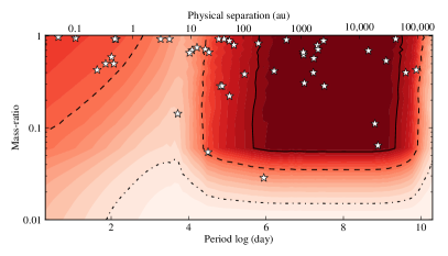
Figure 1: Average detection probabilities (contours from red, 100% to white, 0%) and detected companions (white stars) in the physical separation versus mass-ratio space for the 49 systems. The solid, dashed and dash-dotted lines encompass areas with detection probabilities $\geq$ 90%, 50% and 10%, respectively.

4 Detection completeness

We did not attempt to correct our statistics with our detection probabilities, however, below we justify why this should not significantly affect our results.

In this analysis before averaging the detection probabilities over the sample, as in Figure 1, we first consider whether a companion is likely to inhabit the parameter space based on stability arguments. Tokovinin (2014b) showed that the region of instability (for triple and higher-order systems), based on the ratio of periods in the system is between certain values ($4.7<P_{L}/P_{S}<47$). We use the mid-value (26) of this criterion to mask regions of detection probability space using previously identified companions in the system. For example, if a system has a companion with a period of 100 day then we mask the region 4–2600 day. Masking in this case means setting a detection probability of 1. This is because we use these probabilities to predict where the missing companions would be and we have indirectly probed this space with our stability arguments. We repeated this for all objects to create a new set of detection probability arrays. We then averaged these detection probabilities over the mass-ratio in each period bin because there is no significant evidence that the mass-ratio is a function of period (Reggiani & Meyer, 2013; Tokovinin, 2014b).

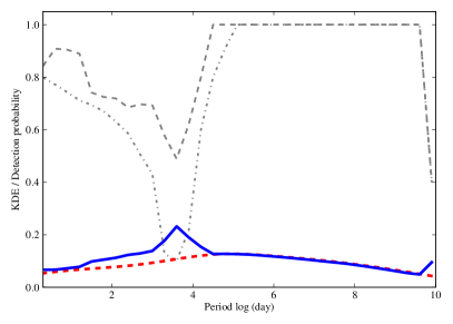
Figure 2: Kernel density estimations for the period versus companion-star fraction. The dashed and dash-dotted grey lines represent median detection probabilities (averaged over mass-ratio) with and without dynamical stability considerations, respectively. The red dashed line is the raw sample analysed in the body of this work and the blue line is the detection-probability corrected distribution.

Figure 2 shows our results based on the period distribution of systems in our sample. We used kernel density estimations (KDEs) to perform this analysis which reduces the phase effect when binning data, see Scott (2009) for details.

The grey dotted and dash-dotted lines are the median detection probabilities with and without dynamical constraints, respectively. This Figure shows that although we are very insensitive in regions $\approx$4 day, due to identified companions in the systems, the likely number of missing companions is not very significant. The red dashed line and blue line are the KDEs of the raw sample and the corrected sample (KDE / detection probability), respectively. We then integrated these curves to calculate the quantitative difference in CSF values. The difference was $\approx$15% i.e. the derived CSF value derived in this work is most likely $\approx$1.17 as opposed to 1.02. This increase would not significantly affect any conclusions presented in this work, in fact this value would put our results in even better agreement with the Class 0 CSF value from Tobin et al. (2016), see Section 6.1 for details.

Table 1: Observtional properties of $\beta$-Pictoris targets studied in this work.

ID	Comp.a	Common ID	R.A.	DEC.	Dist.	V	K	Mem. ref.	2MASS lim.	AO refs.	RV refs.
			hh:mm:ss.s	dd:mm:ss	(pc)	(mag.)	(mag.)		(″)
BPC 10	A	V1005 Ori	04:59:34.8	+01:47:01.0	25.9	10.11	6.26	28	4000	3, 2, 8, 12, 17, 19, 24	9, 1, 12
BPC 10	B	2MASS J05015665+0108429	05:01:56.7	+01:08:43.0	25.9	12.87	7.68	11	4000
BPC 12	A	HIP 23418aa	05:01:58.8	+09:58:59.0	33.2	11.67	6.37	20, 28	1000	10
BPC 14	A	BD-21 1074b	05:06:49.5	-21:35:04.0	20.2	11.30	6.11	20, 28	6000	8	12, 9, 12
BPC 16	B	2MASS J05200029+0613036	05:20:00.3	+06:13:04.0	67.8	11.42	8.57	28	600	10	9
BPC 16	A	RX J0520.5+0616	05:20:31.8	+06:16:11.0	71.0	11.64	8.57	28	600	10	9
BPC 16	C	2MASS J05195327+0617258	05:19:53.3	+06:17:26.0	71.0	18.31	12.41	11	600
BPC 19	A	Beta Pic	05:47:17.1	-51:03:59.0	19.4	3.85	3.53	28	4500	7, 26, 3, 29
BPC 2	A	GJ 3076	01:11:25.4	+15:26:21.0	19.3	13.96	8.21	20	5000		20
BPC 22	A	TWA22	10:17:26.9	-53:54:27.0	17.6	13.89	7.69	28	5500	12, 7, 2	9, 12
BPC 26	A	V824 Ara	17:17:25.5	-66:57:04.0	31.4	6.86	4.70	28	3100	23, 7, 2, 19, 24	25
BPC 26	B	HD 155555 c	17:17:31.3	-66:57:06.0	31.4	12.89	7.63	28	3100	3
BPC 28	A	GSC 08350-01924	17:29:20.7	-50:14:53.0	66.3	12.96	7.99	20, 28	350	10
BPC 3	A	Barta 161 12	01:35:13.9	-07:12:52.0	37.9	13.43	8.08	20, 16	2500		20
BPC 3	B	2MASS J01354915-0753470	01:35:49.2	-07:53:47.0	37.9	13.79	9.81	11	2500
BPC 30	A	HD 161460	17:48:33.7	-53:06:43.0	71.0	8.99	6.78	28	600	10, 7	22
BPC 30	B	2MASS J17483374-5306118	17:48:33.8	-53:06:12.0	71.0	13.65	9.27	11	600
BPC 31	A	HD 164249	18:03:03.4	-51:38:56.0	48.1	7.01	5.91	28	2000	7, 26	12, 9, 11, 12
BPC 31	C	2MASS J18011138-5125594	18:01:11.3	-51:26:00.0	48.1	14.79	11.27	11	2000
BPC 36	A	2MASS J18420694-5554254	18:42:06.9	-55:54:25.0	51.9	13.54	8.58	20	500		20
BPC 36	B	2MASS J18420483-5554126	18:42:04.8	-55:54:13.0	51.9	15.11	9.85	11	500
BPC 37	A	HD 172555	18:45:26.9	-64:52:17.0	28.5	4.80	4.30	28	3500	7, 3, 2, 29, 26, 24
BPC 37	B	CD-64 1208	18:45:37.0	-64:51:46.0	28.5	9.97	6.10	28	3500	24, 7, 2, 19	22
BPC 39	B	Smethells 20	18:46:52.6	-62:10:36.0	52.4	12.20	7.85	20, 28	2000	10, 3	27, 9
BPC 39	A	2MASS J18480637-6213470	18:48:06.5	-62:13:47.0	52.4	7.29	6.14	11	2000
BPC 4	B	HIP 10679	02:17:24.7	+28:44:30.0	27.3	7.78	6.26	28	2500	3, 5	25
BPC 4	A	HD 14082	02:17:25.3	+28:44:42.0	34.5	7.04	5.79	28	2500		25
BPC 4	C	2MASS J02160734+2856530	02:16:07.3	+28:56:53.0	34.5	15.74	11.61	11	2500
BPC 41	A	PZ Tel	18:53:05.9	-50:10:50.0	51.5	8.42	6.37	28	1900	3, 24, 19	12, 12
BPC 42	A	TYC 6872-1011-1	18:58:04.2	-29:53:05.0	82.6	11.73	8.02	20, 28	300	10	11
BPC 42	B	2MASS J18580464-2953320	18:58:04.6	-29:53:32.0	82.6	12.85	8.76	11	300
BPC 43	A	CD-26 13904	19:11:44.7	-26:04:09.0	78.9	10.24	7.37	28	600	10	9, 11
BPC 44	A	Eta Tel	19:22:51.2	-54:25:26.0	48.2	5.17	5.01	28	2000	23, 18, 3, 6, 29
BPC 44	B	HD 181327	19:22:58.9	-54:32:17.0	51.8	7.05	5.91	28	2000	7, 3	9, 12
BPC 47	B	UCAC3 116-474938	19:56:02.9	-32:07:19.0	58.4	13.27	8.11	20, 28	1800	3, 4	27, 20, 11
BPC 47	A	TYC 7443-1102-1	19:56:04.4	-32:07:38.0	56.3	11.78	7.85	20, 28	1800	8, 3, 4	27, 9, 11
BPC 52	C	AU Mic	20:45:09.5	-31:20:27.0	9.8	8.80	4.53	28	10000	23, 15, 2, 8, 17, 14, 3, 5, 24	12, 9, 1, 12
BPC 52	B	AT Mic S	20:41:51.1	-32:26:10.0	9.5	10.89	4.94	28	10500	24, 2, 19	1, 12
BPC 52	A	AT Mic N	20:41:51.2	-32:26:07.0	10.2	10.89	4.94	28	10500	23, 15, 2, 3, 19, 24	1, 12
BPC 55	A	2MASS J20434114-2433534 A	20:43:41.1	-24:33:53.0	45.1	14.45	7.76	20	2200		20
BPC 55	B	2MASS J20434114-2433534 B	20:43:41.1	-24:33:53.0	45.1	14.45	7.76	28	2200		20
BPC 57	A	HD 199143	20:55:47.7	-17:06:51.0	45.7	7.33	5.81	28	1200	23, 21
BPC 57	B	AZ Cap	20:56:02.7	-17:10:54.0	45.7	10.62	7.04	20, 28	1500	23, 24, 19	9
BPC 6	B	BD+30 397 b	02:27:28.1	+30:58:41.0	40.0	12.39	7.92	28	2400	5	11
BPC 6	A	AG Tri	02:27:29.3	+30:58:25.0	40.0	10.15	7.08	28	2400	5	11, 1
BPC 63	A	WW PsA	22:44:58.0	-33:15:02.0	23.6	12.10	6.93	28	4800	8	9, 20, 1
BPC 63	B	TX PsA	22:45:00.0	-33:15:26.0	20.1	13.35	7.79	28	4800	8, 10, 3	9, 1
BPC 65	C	G 271-110	01:36:55.1	-06:47:38.0	29.5	…	8.86	20	4100	4
BPC 65	B	2MASS J01373545-0645375	01:37:35.4	-06:45:38.0	24.0	7.68	5.75	11	4100	14, 24, 17	12
BPC 65	A	2MASS J01334282-0701311	01:33:42.8	-07:01:31.0	29.5	5.77	4.26	11	4100		27
BPC 68	A	2MASS J14142141-1521215	14:14:21.4	-15:21:21.5	30.2	10.39	6.60	20	3200	7	27, 20
BPC 68	B	2MASS J14141700-1521125	14:14:17.0	-15:21:13.0	30.2	15.60	8.82	11	3200
BPC 69	B	2MASS J21212873-6655063	21:21:28.7	-66:55:06.3	30.2	10.66	7.01	20	3200
BPC 69	A	2MASS J21212446-6654573	21:21:24.5	-66:54:57.0	30.2	9.00	6.40	11	3200	15
BPC 70	A	2MASS J20100002-2801410	20:10:00.0	-28:01:41.0	48.0	15.13	7.73	20	2700	4	20
BPC 70	B	2MASS J20085122-2740536	20:08:51.1	-27:40:54.0	48.0	16.27	11.78	11	2700
BPC 8	A	EXO 0235.2-5216	02:36:51.7	-52:03:04.0	28.6	12.07	7.50	20, 28	3500	23, 6	27, 20
BPC 9	A	HD 29391	04:37:36.1	-02:28:25.0	29.4	5.22	4.54	28	3400	26, 3, 13
BPC 9	B	2MASS J04373746-0229282	04:37:37.5	-02:29:28.0	29.4	10.64	6.41	11	3400	8, 15	27, 9, 1, 12

Bailey et al. (2012): 1, Biller et al. (2007): 2, Biller et al. (2013): 3, Bowler et al. (2015): 4, Brandt et al. (2014): 5, Chauvin et al. (2003): 6, Chauvin et al. (2010): 7, Delorme et al. (2012): 8, Elliott et al. (2014): 9, Elliott et al. (2015): 10, Elliott et al. (2016): 11, Elliott et al. in prep.: 12, Heinze et al. (2010): 13, Janson et al. (2013): 14,Kasper et al. (2007): 15, Kraus et al. (2014): 16, Lafrenière et al. (2007): 17, Lowrance et al. (2005): 18, Masciadri et al. (2005): 19, Malo et al. (2014): 20, Metchev & Hillenbrand (2009): 21, Messina et al. (2010): 22, Neuhäuser et al. (2003): 23,Nielsen & Close (2010): 24, Nordström et al. (2004): 25, Rameau et al. (2013): 26, Kordopatis et al. (2013): 27,Torres et al. (2006): 28, Vigan et al. (2012): 29 ^aThe "ID" column + "Comp." column is a unique identifier for resolved targets. This unique identifier links this Table to Table 2, this avoids any confusion for targets with multiple unresolved components.

5 Defining wide multiple systems in the young moving groups

Wide components are usually identified from the galactic motion (the quantity used, at least in initial identification, is proper motion) they share with their associated primary. With the proper motion, radial velocity and either a photometric or kinematic distance, the 3D kinematics can be derived. However, young moving group members are also classified on this basis, i.e. looking for collections of objects sharing the same galactic motion. Therefore we need to clarify what is a component in a multiple system and what is another moving group member.

To investigate this we looked at the different scales of physical clustering within the BPMG. We cannot use projected separations from spatial positions for this analysis as the proximity of the stars means the group has significant depth (in galactic co-ordinates: X$\approx$160, Y$\approx$100, Z$\approx$45 pc). We can, however, use the derived photometric distances to known members and perform queries in a 3D spatial volume. This is similar to the analysis presented in Larson (1995) where the authors identified a break in the density of objects as a function of angular separation in Taurus (58″, $\approx$8000 au). However, as the depth of Taurus is significantly lower ($\approx$20 pc) an angular query was sufficient, assuming a fixed distance to all sources.

For our analysis we queried a 30 pc volume around each bona-fide member of the BPMG using the derived $X$, $Y$ and $Z$ galactic positions. We calculated the magnitude of the distance difference $\sqrt{(X_{1}-X_{2})^{2}+(Y_{1}-Y_{2})^{2}+(Z_{1}-Z_{2})^{2}}$ between the considered bona-fide member and any other member in this volume. For wide components that share statistically similar radial velocities and proper motions and without $X$, $Y$ and $Z$ values, the distance magnitude is computed from the angular separation of the components and the distance to the bona-fide member. We collected all of these distance magnitudes together and analysed the resultant distribution, shown in Figure 3. Note that the sum of separation bins ($\approx$900) is much larger than the input sample (70) because there is a lot of overlapping parameter space from query to query (for example if all 70 objects had 10 other members within the 30 pc volume this would result in a sum of 700 objects in the distribution).

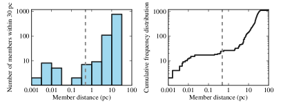
Figure 3: Left panel: The number of members within a 30 x 30 x 30 pc volume of space for each member of the BPMG, summed over the population as a function of the physical separation. Right panel:

In Figure 3 we see that there are two components in the distribution. We also show the 100,000 au limit ($\approx$0.5 pc), the widest companions we are sensitive to from the limits derived in Elliott et al. (2016). We do not attempt to fit any power-laws to the components observed in the right panel of Figure 3 as in Larson (1995). The BPMG sample is far from complete and there are likely still many lower-mass members to be identified (similar to the Tuc-Hor moving group, see Kraus et al. 2014). Additionally our detection limit of 100,000 au means at this point we are no longer sensitive to identifying wide companions and therefore any analysis of the resultant distribution is problematic.

We use Figure 3 to demonstrate that there are at least two different spatial scales (breaking at $\approx$1-5 pc), demonstrated clearly in the right panel. This break in the typical spatial density of members in BPMG is evidence that the population of identified wide companions (100,000 au and smaller) is not just a continuation of clustering down to smaller scales. These wide companions form a distinct population, their separation distribution is a result of a different physical process.

6 Results

In the following section we present analysis using the multiplicity fraction (MF) defined by

$$MF=\frac{B+T+Qu+Qi+Se...}{S+B+T+Qu+Qi+Se...}$$ (1)

and the companion-star fraction (CSF), defined by

$$CSF=\frac{B+2T+3Qu+4Qi+5Se...}{S+B+T+Qu+Qi+Se...}$$ (2)

where S, B, T, Qu, Qi, Se represent the number of single, binary, triple, quadruple, quintuple and sextuple systems, respectively.

Additionally we use the physical separation (a proxy for the semi-major axis) versus CSF which allows us to investigate the dynamical evolution of multiple systems.

Table 2: Multiple systems used in this work.

ID	Comp.	Struc.	Hier.	M1	M2	Sep.	Typea	Ref.
				(M⊙)	(M⊙)	(au)
BPC 10	B	A, B, *	L1	0.70	0.30	81044	Cpm	EL16
BPC 10	A	Aa, Ab, A	L11	0.70	0.30	0.26	s	EL14
BPC 12	A	A, B, *	L1	0.50	0.40	46	v	HIP
BPC 12	A	Aa, Ab, A	L11	1.00	0.95	0.10	S	DE99
BPC 14	B	A, B, *	L1	0.60	0.50	122	v	WDS
BPC 14	A	Ba, Bb, B	L12	0.30	0.20	13	v	WDS
BPC 16	C	A, B, *	L1	0.70	0.70	39269	Cpm	EL16
BPC 16	A	Aa, Ab, A	L11	0.70	0.20	28	v	EL15
BPC 19	A	A, B, *	L1	1.40	0.01	7.78	v	WDS
BPC 2	A	A, B, *	L1	0.10	0.07	5.79	v	WDS
BPC 22	A	A, B, *	L1	0.10	0.10	1.76	v	WDS
BPC 26	B	A, B, *	L1	1.30	0.40	1065	v	AF15
BPC 26	A	Aa, Ab, A	L11	1.30	1.04	0.94	s	WDS
BPC 28	A	A, B, *	L1	0.63	0.56	48	v	EL15
BPC 3	A	Aa, Ab, A	L1	0.20	0.20	0.38	s	MA14
BPC 30	A	Aa, Ab, A	L1	1.30	1.27	0.71	s	ME10
BPC 31	B	Aa, Ab, A	L1	1.20	0.50	323	v	WDS
BPC 36	B	A, B, *	L1	0.50	0.20	1138	Cpm	WDS
BPC 37	B	A, B, *	L1	0.50	0.70	2035	v	WDS
BPC 37	B	Ba, Bb, B	L12	0.70	0.10	5.71	v	WDS
BPC 37	B	Ba1, Ba2, Ba	L121	0.70	0.70	0.86	s	ME10
BPC 39	A	A, B, *	L1	1.30	0.70	28894	v	AF15
BPC 39	A	Aa, Ab, A	L11	1.30	0.65	1.57	s	MO13
BPC 4	B	Aa, Ab, A	L1	1.10	1.00	390	v	WDS
BPC 41	A	A, B, *	L1	1.10	0.06	21	v	WDS
BPC 41	A	Aa, Ab, A	L11	1.10	0.65	1.54	s	NO04
BPC 42	B	A, B, *	L1	0.90	0.80	2290	Cpm	AF15
BPC 43	A	A, B, *	L1	1.03	0.74	21	v	EL15
BPC 44	B	A, B, *	L1	1.40	0.09	20072	Cpm	WDS
BPC 44	B	Aa, Ab, A	L11	1.40	0.04	203	v	WDS
BPC 47	B	A, B, *	L1	0.70	0.40	1488	Cpm	WDS
BPC 47	B	Ba, Bb, B	L12	0.40	0.30	11	v	WDS
BPC 47	B	Ba1, Ba2, Ba	L121	0.40	0.40	0.56	s	MA14
BPC 52	C	A, B, *	L1	0.50	0.20	44377	Cpm	EL16
BPC 52	C	Ba, Bb, B	L12	0.20	0.20	27	Cpm	WDS
BPC 55	B	A, B, *	L1	0.60	0.60	4.51	v	MA13
BPC 55	A	Aa, Ab, A	L11	0.60	0.30	1.35	s	ELPP
BPC 57	B	A, B, *	L1	1.30	0.90	14764	Cpm	WDS
BPC 57	A	Aa, Ab, A	L11	0.90	0.20	50	v	WDS
BPC 57	B	Ba, Bb, B	L12	1.30	0.50	100	v	WDS
BPC 6	B	A, B, *	L1	0.80	0.50	894	Cpm	AF15
BPC 63	B	A, B, *	L1	0.30	0.20	681	Cpm	SO02
BPC 65	C	Ba, Bb, B	L12	0.90	0.10	14635	Cpm	WDS
BPC 68	B	A, B, *	L1	0.70	0.20	1905	Cpm	WDS
BPC 68	A	Aa, Ab, A	L11	0.70	0.20	33	v	WDS
BPC 69	A	Aa, Ab, A	L1	0.80	0.80	0.30	s	TO06
BPC 70	A	Aa, Ab, A	L1	0.70	0.70	34	v	WDS
BPC 8	A	Aa, Ab, A	L1	0.40	0.20	0.29	s	ELPP
BPC 9	B	A, B, *	L1	1.40	1.11	1957	Cpm	FE06
BPC 9	B	Ba, Bb, B	L12	0.67	0.44	8.83	V	MO15

^aCpm: Common proper motion companion, s: spectroscopic binary without orbital solution, S: spectroscopic binary with orbital solution, v: visual binary without orbital solution, V: visual binary with orbital solution. HIP: Perryman et al. (1997), DE99: Delfosse et al. (1999), WDS: Mason et al. (2001), SO02: Song et al. (2002), NO04: Nordström et al. (2004), Torres et al. (2006), ME10: Messina et al. (2010), BA12: Bailey et al. (2012), MA13: Malo et al. (2013), MA14: Malo et al. (2014), EL14: Elliott et al. (2014), EL15: Elliott et al. (2015), AF15: Alonso-Floriano et al. (2015), MO15: Montet et al. (2015), EL16: Elliott et al. (2016), ELPP: Elliott et al. in prep.

6.1 Linking multiplicity: young - old populations

The MF and CSF of the BPMG, shown in row four of Table 3, are incompatible with that of the older field population, at $>5\sigma$ level. In contrast, our derived quantities are compatible with those of extremely young Class 0 sources from the work of Chen et al. (2013) ($a\approx$50-5000 au) and Tobin et al. (2016) ($a\approx$15-10,000 au). However, we are sensitive to a much wider range of physical separations. Therefore, the apparent conservation of the MF and CSF values between these regions can be interpreted as an evolution of the separation distribution. Assuming all considered regions have statistically similar primordial multiple system populations (Kroupa, 2011), we investigate if significant dynamical evolution from Class 0 (Perseus), to Class I/II/III (Taurus), to Class III (BPMG), to main sequence (the field) populations can explain the derived quantities.

The top panel of Figure 4 shows the CSF as a function of physical separation for Class 0 objects in Perseus (Tobin et al., 2016). We chose the Tobin et al. (2016) sample as our main comparison to Class 0 sources as opposed to Chen et al. (2013) because of its completeness and focus on one specific region, the Perseus region. The main limitation of the observations of Perseus is the angular resolution (0.″065, $\approx$15 au, grey line). However, we would not expect to find components smaller than this separation due to the opacity limit, where the compression becomes approximately adiabatic, of the initial cores ($\approx$5 au, Larson 1969). If components have undergone significant dynamical evolution at this stage already (as suggested by Reipurth et al. 2010) and are brought within this limit they would most likely have merged. Additionally systems with separations greater than $\sim$5,000-10,000 au at these young ages, are unlikely primordial (originating from different birth sites). We cannot assess whether components are gravitationally bound however, as in Tobin et al. (2016), we treat all identified components within 10,000 au as bound systems. The second panel shows the distribution for the Taurus region (3-5000 au). We see that there is a wealth of systems with separations $<$10 au and the overall number of multiple systems is still very high.

Table 3: A summary of the type and fraction of multiple systems samples analysed in this work. S:B:T:Qu:Qi:Se represent system components from Equation 1.

Sample	Ref.	S:B:T:Qu:Qi:Se	Total	MFa	CSFa
Class 0 regions	1	36:43:15:6:0:0	33	0.64${}^{+0.09}_{-0.05}$	0.91${}^{+0.15}_{-0.09}$
Perseus	2	43:23:17:7:7:3	30	0.57${}^{+0.06}_{-0.11}$	1.20${}^{+0.27}_{-0.32}$
Taurus	3	41:43:10:3:0:1	117	0.59${}^{+0.04}_{-0.04}$	0.78${}^{+0.09}_{-0.07}$
BPMG	4	35:35:24:6:0:0	49	0.65${}^{+0.06}_{-0.02}$	1.02${}^{+0.14}_{-0.06}$
BPMG (10,000 au)	4	44:42:11:3:0:0	57	0.56${}^{+0.07}_{-0.05}$	0.73${}^{+0.12}_{-0.08}$
BPMG (1000 au)	4	52:38:10:0:0:0	63	0.48${}^{+0.06}_{-0.07}$	0.58${}^{+0.08}_{-0.09}$
The field	5	56:33:8:3:0:0	454	0.44${}^{+0.01}_{-0.02}$	0.58${}^{+0.01}_{-0.04}$
The field	6	54:33:8:4:1:0	4847	0.46${}^{+0.01}_{-0.01}$	0.65${}^{+0.01}_{-0.01}$

^a$1\sigma$ confidence intervals from 1000 bootstrapped samples. Note, bootstrapped uncertainties are indistinguishable from those calculated using binomial statistics for MF values in the majority of cases.
1: Chen et al. (2013), 2: Tobin et al. (2016), 3: Kraus et al. (2011), 4: This work, 5: Raghavan et al. (2010), 6: Tokovinin (2014b)

For comparison with the BPMG (middle panel of Figure 4) we assume all wide systems are primordial. There is another mechanism to produce wide (non-primordial) systems (Kouwenhoven et al., 2010), which is discussed in Section 8. At the same time as there being a wealth of systems with separations $<$10 au in our sample there are also many objects with large separations (1000-100,000 au). This stretching of the initial separation distribution to both smaller separations and larger separations implies intense dynamical evolution.

6.2 The role of unfolding higher-order systems

Reipurth & Mikkola (2012) described a potential physical mechanism for the formation of wide and very wide binaries ($\geq$1,000 au); through the dynamical unfolding of primordial triple systems. The mechanism predicts:

• A preference for wide binaries to be in triple systems

• These systems will have high ($>$0.9) eccentricities.

• The majority of wide components will be low-mass (these systems are likely unstable and therefore their lifetime is $<$100 Myr)

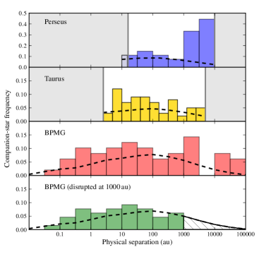
Figure 4: Physical separation versus CSF for four different samples. Top: Perseus (15-10,000 au, Tobin et al. 2016), second: Taurus (3-5000 au, Kraus et al. 2011), third: The BPMG sample, bottom: The BPMG sample, disrupted at 1000 au. The log-normal field distribution derived in Raghavan et al. (2010) is over-plotted (black dotted line) in all panels. Grey shaded areas represent parameter spaces not probed.

We note that although there should be a preference for wide binary systems to be in triple systems we would not expect to find all systems in this configuration due to previous mergers. Additionally that we cannot assess the eccentricity of the wide components. This problem is discussed in more detail in Section 8.

6.2.1 Higher-order multiplicity in wide systems?

We found that for systems with companions $>$1000 au and $>$10,000 au, 11 / 14 (0.79${}^{+0.07}_{-0.14}$) and 6 / 7 (0.86${}^{+0.05}_{-0.21}$) were part of triple or higher-order systems, respectively. In contrast, for systems with no components $>$1000 au we found 4 / 19 (0.21${}^{+0.12}_{-0.06}$) systems were higher-order systems. The fraction of higher-order multiple systems is clearly a function of the physical separation.

Additionally we looked at the separations of the inner components of the 11 systems (8 triples, 3 quadruples, i.e. 14 inner components) with companions $>$1000 au. Of these 14, 11 had separations smaller than the inner peak identified of the separation distribution found in the Perseus region by Tobin et al. (2016). Again, this supports the theory of migration via the interaction of multiple components.

Although there is no evidence for higher-order multiplicity amongst the 3 binary systems (BPC 36,42,65) that have components $>$1000 au, that does not necessarily negate the possibility, as few of the components have been observed with AO-imaging and have multi-epoch radial velocity data, see Table LABEL:tab:sample_targets.

6.2.2 Masses and mass-ratios

We studied the mass distribution within the 10 higher-order multiple systems with wide components. For the triple systems we compared the mass-ratios of the inner binaries and outer components. In the case of the quadruple systems we compared the mass-ratios of each sub-system and each component with that of the primary. In neither case we found a significant relationship between the system configuration and absolute mass nor the mass-ratio. Our derived mass-ratio distribution was statistically similar to a power-law with $\gamma=0$ i.e. a flat distribution in the range 0.1-1.0.

6.3 Disruption of higher-order systems

In the framework of Reipurth & Mikkola (2012) we estimated the survival rate of the identified triple systems, given their mass distribution.

Similar to Figure 3 of Reipurth & Mikkola (2012) we compared the mass sum of the inner binary ($M_{a}+M_{b}$) to the mass of the outer companion ($M_{c}$) for wide triple systems. We show our results in Figure 5: star markers are BPMG triple systems with at least one companion $>$1000 au, grey dots are field stars (Tokovinin, 2014b) meeting the same criterion. Firstly we see that all BPMG systems are in the dominant binary (red shaded area) regime. Secondly, we see that 5 / 8 of these systems occupy a parameter space mostly uninhabited by very wide field systems. Reipurth & Mikkola (2012) show that most systems in this parameter space are unstable and are disrupted between the ages of 10-100 Myr. Therefore, our results imply that the majority of wide triple systems in the BPMG are in the process of disintegrating/decaying without external influence.

To investigate if the disruption of higher-order multiple systems in our sample could “bridge-the-gap" between young populations rich in multiplicity and the older processed field population we artificially disrupted our higher-order multiple systems at two physical separation limits (1000 au and 10,000 au). The first limit is a somewhat arbitrary definition of a wide binary, the second is an approximation for the size of a hydrostatic clump. We then calculated the MF and CSF, considering systems with components wider than these limits as separate systems. The results are shown in Table 3. Considering the limit at 10,000 au, the MF and CSF values are within 2 $\sigma$ and 1 $\sigma$, respectively, of the field population (higher in value). For the limit at 1000 au both the MF and CSF values are within 1$\sigma$ ( the CSF now lower in value). In the same line, the MF and CSF values of Taurus are compatible with the disruption of systems at 10,000 au in the BPMG sample. This suggests that the majority of primordial systems with separations somewhere between 1000-10,000 au and beyond have been destroyed or decayed in older populations.

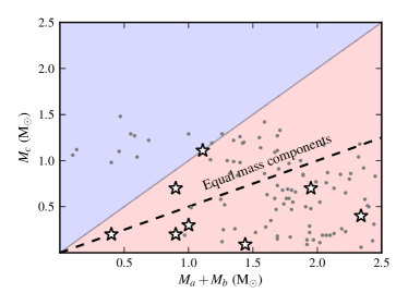
Figure 5: Inner binary ($M_{a}+M_{b}$) versus outer component ($M_{c}$) masses for BPMG (stars) and field (Tokovinin (2014b), grey dots) wide systems. The blue and red shaded areas highlight the dominant single and binary regimes, respectively. The dotted line describes equal mass component systems (Ma = Mb = Mc).

We also compared the CSF, as a function of physical separation distribution, for: the original BPMG sample, the BPMG sample disrupted at 1000 au and 10,000 au and the field. The results are shown in Figure 6. We split our samples at the mean of the field distribution ($\approx$50 au) and compared the different populations. We would expect the distribution of inner separations to be very similar already at the age of the BPMG, as demonstrated in Elliott et al. (2014); Elliott et al. (2015). In the left panel of Figure 6 we show that the distributions are indeed very similar. The apparent difference at $\approx$0.3 au is most likely an artefact of the assignment of physical separation values to spectroscopic systems currently without orbital solutions.

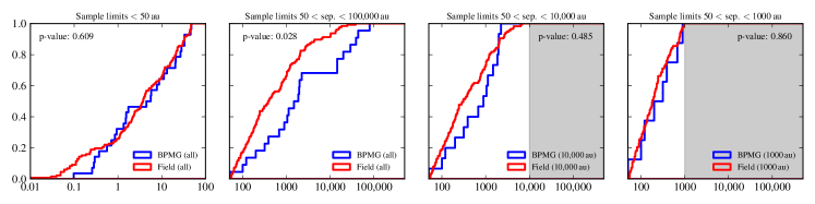
Figure 6: Cumulative separation distributions for four different samples. Labels above each plot indicate the physical separation range. The p-value calculated from the Kolmogorov-Smirnov test is shown in each panel. Field systems from from Raghavan et al. (2010).

We can reject the null hypothesis when comparing the field with the original BPMG sample (p-value 0.028, second panel of Figure 6) for separations $>$50 au, i.e. these distributions are not likely to be realisations of the same parent distribution. However, if we compare the BPMG sample disrupted at 1000 and 10,000 au ($3^{\rm rd}$ and $4^{\rm th}$ panel of Figure 6) to the field, we calculate p-values of 0.860 and 0.485, respectively (non rejection).

The recent work of Parker & Meyer (2014) suggested that the primordial binary population is similar to the population we observe today and has undergone little dynamical processing. Along with many previous works, Parker & Meyer (2014) have focussed on binaries as opposed to higher-order multiple systems. However, our results indicate that the disruption of primordial higher-order systems significantly shapes older, more processed populations, such as the field. We outline a simple model for the contribution of unfolding triple systems to the separation distribution in a population in Section 7.

7 A model for the dynamical evolution of triple systems

Below we collect together the physical mechanisms discussed in the previous sections, along with additional physics, to briefly outline the separation evolution of higher-order (in this case, specifically triple) systems in a population. Our simplified model is shown in Figure 7 in 3 stages.

Stage I: We approximate the initial distribution of separations within clumps using the identified bimodal distribution of Tobin et al. (2016) (peaks; 75 and 3000 au). These peaks have been attributed with typical scales for disc ($\sim$100 au, Zhu et al. 2012) and core ($\sim$1000 au, Offner et al. 2010) fragmentation. No multiple systems can inhabit the hatched region for separations $<$10 au due to the size of the first Larson core (a pressure supported fragment) ($\approx$5 au, Larson, 1969). The second hatched region beyond $\approx$5000-10,000 au represents the initial size of the hydrostatic clump (Benson & Myers, 1989; Motte et al., 1998; Pineda et al., 2011), i.e. by definition a primordial multiple system at this stage cannot have components beyond this separation.

Stage II: The inner peak both broadens and shifts to closer separations through the exchange of angular momentum with the outer component (components are now in a hierarchical configuration, although potentially unstable, as Reipurth & Mikkola 2012). This is supported by the conservation of the MF and CSF quantities in larger separation ranges for Class 0 sources (15-10,000 au, Tobin et al. 2016), Class I/II/III sources (3-5000 au, Kraus et al. 2011) and Class III sources ($\approx$0.01-100,000 au, this work). Additional migration to closer separations can also occur through gas-induced orbital decay (Korntreff et al., 2012; Bate, 2012). Concurrently, through angular momentum exchanges, the outer components move to wider separations. These wide components (red shaded area) are weakly bound, and some will be in the process of decaying (so-called unfolding: Reipurth & Mikkola 2012) without any external influence. Others may be dynamically disrupted / destroyed by external dynamics i.e. stellar encounters within a cluster. Our analysis in Section 6.3 indicates that most systems are in the process of decaying without external influence. However, as this process is still taking place at the age of the BPMG, there is still a significant population of wide systems.

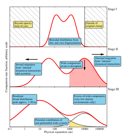
Figure 7: A simplified model of the dynamical evolution of separations within a population of primordial triple systems. Regions of interest are annotated and processes are described in detail in the text (Section 7).

Stage III: In loose low-density environments, such as the BPMG, the resultant distribution is double peaked. The inner peak is at a smaller separation than the original 75 au ($\approx$4 au for the higher-order multiple systems in our sample). The outer peak ($\approx$8000 au in our sample) is smaller as some components have unfolded and decayed completely, reducing the number of triples. However, a significant population still remains, due to the lack of external dynamical perturbations. We have highlighted the region (gold shaded area) where non-primordial wide multiple systems can be formed during the cluster dissolution phase (Kouwenhoven et al. 2010, discussed in Section 8). In the case of higher-density and older ($\approx$100 Myr) environments, the secondary peak is mostly destroyed and the contribution of primordial triple systems to the overall distribution is small/negligible.

8 Discussion and limitations

We have shown that the dynamical evolution of primordial higher-order multiple systems can reconcile the multiplicity properties of Perseus, Taurus, BPMG and the field. Below we discuss the current limitations and prospects.

The mechanism of Kouwenhoven et al. (2010) is a potential route to produce wide, non-primordial binaries in the cluster dissolution phase. However, this mechanism predicts only one or two wide binaries ($>$1000 au) in a population of the size studied here, compared to the 14 identified. Additionally we have shown how the decay of primordial higher-order systems can “bridge-the-gap" between young and old populations. We do not claim the mechanism of Kouwenhoven et al. (2010) is ineffective, rather that it is not the dominant mechanism in our sample. However, one also has to consider that binary formation and destruction is very stochastic. N-body simulations of clusters with very similar initial conditions can produce resultant distributions with different forms (Parker & Goodwin, 2012). Therefore, we must conduct similar analysis on other nearby young moving groups in order to see if those populations also have similar multiplicity properties to the BPMG.

A parameter that would help to determine the formation mechanism of wide multiple systems is their eccentricity ($e$). A natural consequence of the Reipurth & Mikkola (2012) mechanism is a distribution peaked at high eccentricities. Whereas the mechanism of Kouwenhoven et al. (2010) predicts a flatter eccentricity distribution, see their Figure 10. Tokovinin & Kiyaeva (2016) recently showed that wide binaries in the field do not have a thermal eccentricity distribution and therefore are unlikely products of either formation scenario. Given the predicted periods of very wide systems ($\gtrsim$ Myr) determining their eccentricities is extremely challenging. However, the gaia mission (Lindegren et al., 2008) will provide extremely accurate astrometry (7-25 $\mu$as) that can help. Face-on multiple systems of total mass 1 M_⊙, at 40 pc, and with 20,000 au separation, will have detectable movement at 3$\sigma$ level using gaia astrometry within 1 yr.

The work of Reipurth & Mikkola (2012) used only three bodies within the original clump to study the formation of wide binaries. However, the initial multiplicity is likely to be a spectrum, which indeed is observed in young regions (Chen et al. 2013, Tobin et al. 2016) where clumps contain up to six components. Higher-order systems would be responsible for an even more chaotic start for components within the clump, likely resulting in more ejections. Further studies of nearby young regions with instruments such as ALMA and the VLA will provide further insight into the initial distributions of hydrostatic cores. These can then be used as realistic starting points of N-body simulations and evolved into older dynamically processed populations.

9 Conclusions

• Similar CSF values between the very young sources of Perseus and the BPMG can be explained by dynamical evolution of the separation distribution of multiple systems.

• The high fraction of wide ($>$1000 au, 11 / 14) and very wide ($>$10,000 au, 6 / 7) systems in higher-order configurations supports the mechanism of Reipurth & Mikkola (2012).

• There is no significant mass-ratio trend among inner and outer components in wide higher-order systems.

• The separation distribution of the field and the BPMG (for separations $>$50 au) are not realisations of the same parent distribution (p-value 0.03).

• The decay of primordial higher-order (triple and higher-order) systems can link multiplicity in young regions to dynamically processed populations such as the field, in opposition to the more static framework of Parker & Meyer (2014).

• The abundance and configuration of the wide systems in the BPMG favours the Reipurth & Mikkola (2012) mechanism over that of Kouwenhoven et al. (2010).

References

- Alonso-Floriano et al. (2015) Alonso-Floriano F. J., Caballero J. A., Cortés-Contreras M., Solano E., Montes D., 2015, A&A, 583, A85
- Bailey et al. (2012) Bailey III J. I., White R. J., Blake C. H., Charbonneau D., Barman T. S., Tanner A. M., Torres G., 2012, ApJ, 749, 16
- Baraffe et al. (2015) Baraffe I., Homeier D., Allard F., Chabrier G., 2015, A&A, 577, A42
- Barrado y Navascués et al. (1999) Barrado y Navascués D., Stauffer J. R., Song I., Caillault J.-P., 1999, ApJ, 520, L123
- Bate (2012) Bate M. R., 2012, MNRAS, 419, 3115
- Bell et al. (2015) Bell C. P. M., Mamajek E. E., Naylor T., 2015, MNRAS, 454, 593
- Benson & Myers (1989) Benson P. J., Myers P. C., 1989, ApJS, 71, 89
- Biller et al. (2007) Biller B. A., et al., 2007, ApJS, 173, 143
- Biller et al. (2013) Biller B. A., et al., 2013, ApJ, 777, 160
- Binks & Jeffries (2014) Binks A. S., Jeffries R. D., 2014, MNRAS, 438, L11
- Bowler et al. (2015) Bowler B. P., Liu M. C., Shkolnik E. L., Tamura M., 2015, ApJS, 216, 7
- Brandt et al. (2014) Brandt T. D., et al., 2014, ApJ, 786, 1
- Caballero (2010) Caballero J. A., 2010, A&A, 514, A98
- Chauvin et al. (2003) Chauvin G., et al., 2003, A&A, 404, 157
- Chauvin et al. (2010) Chauvin G., et al., 2010, A&A, 509, A52
- Chen et al. (2013) Chen X., et al., 2013, ApJ, 768, 110
- Cutri et al. (2003) Cutri R. M., et al., 2003, VizieR Online Data Catalog, 2246, 0
- Delfosse et al. (1999) Delfosse X., Forveille T., Beuzit J.-L., Udry S., Mayor M., Perrier C., 1999, A&A, 344, 897
- Delorme et al. (2012) Delorme P., Lagrange A. M., Chauvin G., Bonavita M., Lacour S., Bonnefoy M., Ehrenreich D., Beust H., 2012, A&A, 539, A72
- Duchêne & Kraus (2013) Duchêne G., Kraus A., 2013, ARA&A, 51, 269
- Elliott et al. (2014) Elliott P., Bayo A., Melo C. H. F., Torres C. A. O., Sterzik M., Quast G. R., 2014, A&A, 568, A26
- Elliott et al. (2015) Elliott P., et al., 2015, A&A, 580, A88
- Elliott et al. (2016) Elliott P., Bayo A., Melo C. H. F., Torres C. A. O., Sterzik M. F., Quast G. R., Montes D., Brahm R., 2016, preprint, (arXiv:1604.03550)
- Heinze et al. (2010) Heinze A. N., Hinz P. M., Sivanandam S., Kenworthy M., Meyer M., Miller D., 2010, ApJ, 714, 1551
- Janson et al. (2013) Janson M., et al., 2013, ApJ, 773, 73
- Kasper et al. (2007) Kasper M., Apai D., Janson M., Brandner W., 2007, A&A, 472, 321
- Kordopatis et al. (2013) Kordopatis G., et al., 2013, AJ, 146, 134
- Korntreff et al. (2012) Korntreff C., Kaczmarek T., Pfalzner S., 2012, A&A, 543, A126
- Kouwenhoven et al. (2010) Kouwenhoven M. B. N., Goodwin S. P., Parker R. J., Davies M. B., Malmberg D., Kroupa P., 2010, MNRAS, 404, 1835
- Kraus et al. (2011) Kraus A. L., Ireland M. J., Martinache F., Hillenbrand L. A., 2011, ApJ, 731, 8
- Kraus et al. (2014) Kraus A. L., Shkolnik E. L., Allers K. N., Liu M. C., 2014, AJ, 147, 146
- Kroupa (2011) Kroupa P., 2011, in Alves J., Elmegreen B. G., Girart J. M., Trimble V., eds, IAU Symposium Vol. 270, Computational Star Formation. pp 141–149 (arXiv:1012.1596), doi:10.1017/S1743921311000305
- Lafrenière et al. (2007) Lafrenière D., et al., 2007, ApJ, 670, 1367
- Larson (1969) Larson R. B., 1969, MNRAS, 145, 271
- Larson (1995) Larson R. B., 1995, MNRAS, 272, 213
- Lindegren et al. (2008) Lindegren L., et al., 2008, in Jin W. J., Platais I., Perryman M. A. C., eds, IAU Symposium Vol. 248, IAU Symposium. pp 217–223, doi:10.1017/S1743921308019133
- Lowrance et al. (2005) Lowrance P. J., et al., 2005, AJ, 130, 1845
- Malo et al. (2013) Malo L., Doyon R., Lafrenière D., Artigau É., Gagné J., Baron F., Riedel A., 2013, ApJ, 762, 88
- Malo et al. (2014) Malo L., Artigau É., Doyon R., Lafrenière D., Albert L., Gagné J., 2014, ApJ, 788, 81
- Masciadri et al. (2005) Masciadri E., Mundt R., Henning T., Alvarez C., Barrado y Navascués D., 2005, ApJ, 625, 1004
- Mason et al. (2001) Mason B. D., Wycoff G. L., Hartkopf W. I., Douglass G. G., Worley C. E., 2001, AJ, 122, 3466
- Messina et al. (2010) Messina S., Desidera S., Turatto M., Lanzafame A. C., Guinan E. F., 2010, A&A, 520, A15
- Metchev & Hillenbrand (2009) Metchev S. A., Hillenbrand L. A., 2009, ApJS, 181, 62
- Montet et al. (2015) Montet B. T., et al., 2015, ApJ, 813, L11
- Motte et al. (1998) Motte F., Andre P., Neri R., 1998, A&A, 336, 150
- Neuhäuser et al. (2003) Neuhäuser R., Guenther E. W., Alves J., Huélamo N., Ott T., Eckart A., 2003, Astronomische Nachrichten, 324, 535
- Nielsen & Close (2010) Nielsen E. L., Close L. M., 2010, ApJ, 717, 878
- Nordström et al. (2004) Nordström B., et al., 2004, A&A, 418, 989
- Offner et al. (2010) Offner S. S. R., Kratter K. M., Matzner C. D., Krumholz M. R., Klein R. I., 2010, ApJ, 725, 1485
- Parker & Goodwin (2012) Parker R. J., Goodwin S. P., 2012, MNRAS, 424, 272
- Parker & Meyer (2014) Parker R. J., Meyer M. R., 2014, MNRAS, 442, 3722
- Perryman et al. (1997) Perryman M. A. C., et al., 1997, A&A, 323, L49
- Pineda et al. (2011) Pineda J. E., Goodman A. A., Arce H. G., Caselli P., Longmore S., Corder S., 2011, ApJ, 739, L2
- Raghavan et al. (2010) Raghavan D., et al., 2010, ApJS, 190, 1
- Rameau et al. (2013) Rameau J., et al., 2013, A&A, 553, A60
- Reggiani & Meyer (2013) Reggiani M., Meyer M. R., 2013, A&A, 553, A124
- Reipurth & Mikkola (2012) Reipurth B., Mikkola S., 2012, Nature, 492, 221
- Reipurth et al. (2010) Reipurth B., Mikkola S., Connelley M., Valtonen M., 2010, ApJ, 725, L56
- Reipurth et al. (2014) Reipurth B., Clarke C. J., Boss A. P., Goodwin S. P., Rodríguez L. F., Stassun K. G., Tokovinin A., Zinnecker H., 2014, Protostars and Planets VI, pp 267–290
- Roeser et al. (2010) Roeser S., Demleitner M., Schilbach E., 2010, AJ, 139, 2440
- Scott (2009) Scott D. W., 2009, Multivariate density estimation: theory, practice, and visualization. Vol. 383, John Wiley & Sons
- Song et al. (2002) Song I., Bessell M. S., Zuckerman B., 2002, ApJ, 581, L43
- Tobin et al. (2016) Tobin J. J., et al., 2016, preprint, (arXiv:1601.00692)
- Tokovinin (2014a) Tokovinin A., 2014a, AJ, 147, 86
- Tokovinin (2014b) Tokovinin A., 2014b, AJ, 147, 87
- Tokovinin (2015) Tokovinin A., 2015, AJ, 150, 177
- Tokovinin & Kiyaeva (2016) Tokovinin A., Kiyaeva O., 2016, MNRAS, 456, 2070
- Tokovinin et al. (2006) Tokovinin A., Thomas S., Sterzik M., Udry S., 2006, A&A, 450, 681
- Torres et al. (2006) Torres C. A. O., Quast G. R., da Silva L., de La Reza R., Melo C. H. F., Sterzik M., 2006, A&A, 460, 695
- Torres et al. (2008) Torres C. A. O., Quast G. R., Melo C. H. F., Sterzik M. F., 2008, Young Nearby Loose Associations. p. 757
- Vigan et al. (2012) Vigan A., et al., 2012, A&A, 544, A9
- Zacharias et al. (2005) Zacharias N., Monet D. G., Levine S. E., Urban S. E., Gaume R., Wycoff G. L., 2005, VizieR Online Data Catalog, 1297, 0
- Zacharias et al. (2012) Zacharias N., Finch C. T., Girard T. M., Henden A., Bartlett J. L., Monet D. G., Zacharias M. I., 2012, VizieR Online Data Catalog, 1322, 0
- Zhu et al. (2012) Zhu Z., Hartmann L., Nelson R. P., Gammie C. F., 2012, ApJ, 746, 110