Angular observables for spin discrimination in boosted diboson final states

Abstract

We investigate the prospects for spin determination of a heavy diboson resonance using angular observables. Focusing in particular on boosted fully hadronic final states, we detail both the differences in signal efficiencies and distortions of differential distributions resulting from various jet substructure techniques. We treat the 2 TeV diboson excess as a case study, but our results are generally applicable to any future discovery in the diboson channel. Scrutinizing ATLAS and CMS analyses at 8 TeV and 13 TeV, we find that the specific cuts employed in these analyses have a tremendous impact on the discrimination power between different signal hypotheses. We discuss modified cuts that can offer a significant boost to spin sensitivity in a post-discovery era. Even without altered cuts, we show that CMS, and partly also ATLAS, will be able to distinguish between spin 0, 1, or 2 new physics diboson resonances at the $2\sigma$ level with 30 fb^-1 of 13 TeV data, for our 2 TeV case study.

I Introduction

The resumption of the Large Hadron Collider (LHC) with proton-proton collisions at 13 TeV has reignited the excitement for a possible discovery of new physics. The higher energies afforded by the increase in energy during Run 2 also place additional importance on the need for robust analysis tools to enable such discoveries in the hadronic enviroment of the LHC. One such suite of analysis techniques is the maturing field of jet substructure Butterworth et al. (2008); Abdesselam et al. (2011); Altheimer et al. (2012, 2014); Adams et al. (2015), which take advantage of large Lorentz boosts of decaying Standard Model (SM) or new physics (NP) particles to reveal their underlying partonic constituents. Jet substructure tools are also invaluable for mitigating pile-up backgrounds at the LHC, allowing the ATLAS and CMS experiments to use primary vertex information and jet substructure methods to discard pile-up contamination of jets resulting from the hard scattering process of interest Aad et al. (2012, 2013).

The special utility of jet substructure techniques as new physics discovery tools was recently highlighted in the ATLAS 8 TeV search for electroweak diboson resonances in fully hadronic final states Aad et al. (2015a). In this analysis, ATLAS observed a 2.5$\sigma$ global significance deviation at about 2 TeV in the reconstructed $WZ$ invariant mass distribution. The corresponding CMS 8 TeV analysis Khachatryan et al. (2014a) does not preclude a possible signal at ATLAS, partly because the two experiments use different reconstruction methods for tagging boosted, hadronically decaying $W$ and $Z$ candidates. The most recent 13 TeV results from ATLAS ATL (2015a) and CMS CMS (2015) in the same fully hadronic diboson decay, however, show no evidence for a continued excess.

If the excess is a new physics signal, numerous studies are needed to characterize the resonance and measure the underlying new physics Lagrangian. First, for self-consistency, the signal must also begin to show up in the semi-leptonic and fully leptonic diboson decays. Observing the excess in these decays is also critical, though, because the exclusive rates for the semi-leptonic and fully leptonic modes will help diagnose the underlying $W^{+}W^{-}$ vs. $W^{\pm}Z$ vs. $ZZ$ nature of the purported resonance, which is difficult to disentangle using only hadronic diboson decays. Currently, ATLAS has searches for electroweak diboson resonances with 8 TeV data in the $\ell\nu\ell\ell$ channel Aad et al. (2014), $\ell\ell jj$ channel Aad et al. (2015b), and the $\ell\nu jj$ channel Aad et al. (2015c), which have been combined with the fully hadronic search in Ref. Aad et al. (2015d). In addition, CMS has searches with 8 TeV data in the $\ell\nu\ell\ell$ channel Khachatryan et al. (2015a) and $\ell\nu jj$ and $\ell\ell jj$ channels Khachatryan et al. (2014b). We remark, however, that the 2 TeV excess seen by ATLAS in the fully hadronic channel is only marginally probed by the analyses targetting semi-leptonic diboson decays, after rescaling the signals that fit the excess by the appropriate leptonic branching fractions Brehmer et al. (2015a).

The current situation with 13 TeV data seems to favor the interpretation that the 2 TeV excess was instead a statistical fluctuation, although the data is not conclusive. Both ATLAS and CMS have retooled their fully hadronic diboson resonance analyses ATL (2015a); CMS (2015) to focus on the multi-TeV regime, adopting different jet substructure methods than those used previously during the 8 TeV run. CMS and ATLAS also search in the $\ell\nu jj$ channel CMS (2015); ATL (2015b), respectively, and ATLAS also has performed analyses in the $\ell\ell jj$ channel ATL (2015c) as well as the $\nu\nu jj$ channel ATL (2015d). Although the integrated luminosity at 13 TeV is only 3.2 fb^-1 for ATLAS and 2.6 fb^-1 for CMS, in comparison to the 20 fb^-1 datasets for each experiment at 8 TeV, naive parton luminosity rescaling from 8 TeV to 13 TeV for the simplest new physics explanations of the 2 TeV excess point to ATLAS and CMS being at the edge of NP exclusion sensitivity (see Figure 8 of ATL (2015a), Figure 4 of ATL (2015b), Figure 4 of ATL (2015d), and Figures 9 and 10 of CMS (2015)).

Beyond the self-consistency requirement to observe the diboson excess in leptonic channels, various new physics models also predict a new dijet resonance as well as $VH$ resonances, where $V$ is a massive electroweak boson and $H$ is the Higgs boson Dobrescu and Liu (2015a, b); Brehmer et al. (2015b); Dobrescu and Fox (2015); Anchordoqui et al. (2015). The corresponding dijet resonance searches from ATLAS 8 TeV data Aad et al. (2015e), CMS 8 TeV data Khachatryan et al. (2015b), ATLAS 13 TeV data Aad et al. (2016a) and CMS 13 TeV data Khachatryan et al. (2015c), as well as $WH$ and $ZH$ resonance searches with 8 TeV ATLAS data Aad et al. (2015f), 8 TeV CMS data Khachatryan et al. (2015d, e, 2016), and 13 TeV ATLAS data ATL (2015e), have all variously been statistically consistent with the SM background expectation, which then provide important model-dependent constraints on new physics interpretations of the 2 TeV excess.

Given the experimental situation, many papers have delved into the model-building details and phenomenological questions that reconcile the original excess with the currently available experimental data. Spin-0 explanations are discussed in context of a Higgs singlet Chen and Nomura (2015a), a two Higgs doublet model Chen and Nomura (2015b); Omura et al. (2015); Chao (2015); Aristizabal Sierra et al. (2015), sparticles Petersson and Torre (2015); Allanach et al. (2015a) or composite scalars Chiang et al. (2015); Cacciapaglia et al. (2015). Spin-1 proposals include composite vector resonances Fukano et al. (2015a); Franzosi et al. (2015); Thamm et al. (2015); Bian et al. (2015a); Fritzsch (2015); Lane and Prichett (2015); Low et al. (2015); Fukano et al. (2015b), generic and effective field theory (EFT) models Cacciapaglia and Frandsen (2015); Allanach et al. (2015b); Bian et al. (2015b); Bhattacherjee et al. (2015) as well as heavy $W^{\prime}$ resonances Xue (2015); Dobrescu and Liu (2015a, b); Gao et al. (2015); Brehmer et al. (2015b); Heeck and Patra (2015); Bhupal Dev and Mohapatra (2015); Deppisch et al. (2015); Aydemir et al. (2015); Awasthi et al. (2015); Ko and Nomura (2015); Collins and Ng (2015); Dobrescu and Fox (2015); Aguilar-Saavedra and Joaquim (2015); Aydemir (2016); Evans et al. (2015); Das et al. (2016), $Z^{\prime}$ resonances Hisano et al. (2015); Alves et al. (2015); Anchordoqui et al. (2015); Faraggi and Guzzi (2015); Li et al. (2015); Wang et al. (2015); Allanach et al. (2015c); Feng et al. (2015) or both Cheung et al. (2015); Cao et al. (2015); Abe et al. (2015a, b); Fukano et al. (2015c); Appelquist et al. (2015); Das et al. (2015). Other NP scenarios include glueballs Sanz (2015), excited composite objects Terazawa and Yasue (2015), and in generic and EFT models Aguilar-Saavedra (2015); Kim et al. (2015); Liew and Shirai (2015); Arnan et al. (2015); Fichet and von Gersdorff (2015); Sajjad (2015).

Although the new physics situation with 13 TeV data is less attractive because the initial dataset does not confirm the excess, the experimental sensitivity with the current luminosity is nonetheless insufficient to make a final conclusion for the original excess. Thus the question about whether the excess is a real signal will simply have to wait for more integrated luminosity.

Apart from the excitement over the original ATLAS diboson excess, however, we are motivated to consider how jet substructure techniques can be used as post-discovery tools for resonance signal discrimination. After the Higgs discovery in 2012, the ATLAS and CMS collaborations began comprehensive Higgs characterization programs, which aim to measure the couplings, mass, width, spin, parity, production modes, and decay modes of the Higgs boson. In particular, much of the spin and parity information about the 125 GeV Higgs boson comes from angular correlations in the $h\to 4\ell$ decay Aad et al. (2015g, 2016b); Khachatryan et al. (2015f, g), where the Higgs candidate can be fully reconstructed and all angular observables can be studied.

For the case of a possible 2 TeV resonance $X$, the exact same analytic formalism for spin characterization used for $h\to 4\ell$ Cabibbo and Maksymowicz (1965); Dell’Aquila and Nelson (1986a, b); Nelson (1988); Gao et al. (2010); Bolognesi et al. (2012) applies to $X\to VV\to 4q$ Kim et al. (2015), which naturally opens up the possibility of designing a jet substructure analysis that targets spin and possibly parity characterization of the $X$ resonance. The $X\to VV\to 4q$ situation is more difficult, however, because it is a priori unknown how well the angular correlations in the final state quarks are preserved after the important effects from showering and hadronization, detector resolution, jet clustering, and hadronic $W$ and $Z$ boson tagging are included. In contrast, the $h\to 4\ell$ decay can be analyzed without the complications from quantum chromodynamics (QCD) and only need to account for virtual $\gamma^{*}/Z$ interference and mild detector effects Chen et al. (2013, 2015, 2014). Our study provides a thorough investigation of these important and difficult complications, and we connect distortions in angular observables with specific jet substructure cuts. Our results show significant differences between the ATLAS and CMS 8 TeV and 13 TeV analyses regarding post-discovery signal discrimination. They also provide useful templates for understanding the differences in sensitivity of the current jet substructure methods to tranversely or longitudinally polarized electroweak gauge bosons. We also make projections for how well the current slate of diboson reconstruction methods will perform with 30 fb^-1 of LHC 13 TeV integrated luminosity. The next obvious course of action would be to design a jet substructure method optimized for both signal significance and post-discovery spin discrimination using the extracted subjets. We leave such work for the future and instead focus on determining the viability of existing jet substructure techniques with regards to spin determination.

In Section II, we review the angular analysis framework for characterizing a resonance decay. We also review the broad classes of jet substructure methods and general challenge of reconstructing angular correlations in the fully hadronic final state and the hadronic environment. In Section III, we detail the 2 TeV case study signal benchmarks, review the 8 TeV and 13 TeV ATLAS and CMS fully hadronic boosted diboson decay selection criteria, and show the differential distributions after implementing these analyses. We also identify specific jet substructure cuts to their effects on the differential distributions. We evaluate the semileptonic analyses in Section IV in a similar manner, highlighting the new distortions that arise when considering semileptonic final states. We present our expectations for model discrimination with 30 fb^-1 of LHC 13 TeV data in Section V and briefly discuss improvements in jet substructure analyses targetting signal discrimination. We conclude in Section VI. In Appendix A, we discuss the inclusive background determination for the ATLAS 13 TeV analysis neeeded in our 13 TeV, 30 fb^-1 projections.

II Reconstructing Angular Correlations in $pp\to X$, $X\to V_{1}V_{2}\to 4q$

II.1 General framework

In this section, we review the general framework for studying angular correlations of a resonance $X$ decaying to two intermediate vector bosons that subsequently decay to four light quarks. We will work in the $X$ rest frame and orient the incoming partons along the $+\hat{z}$ and $-\hat{z}$ axes as usual. We also neglect the masses of our final state particles, which reduces the nominal sixteen final state four-momentum components to twelve. Four-momentum conservation in the rest frame of the resonance further reduces the number of independent components to eight. Finally, the overall system can be freely rotated about the $+\hat{z}$ axis, so we can completely characterize the kinematics of the system with seven independent variables, which are five angles and the two intermediate vector masses. If the resonance mass is not known, it also counts as an independent quantity. Finally, if the final state particles are not massless, then their four masses also have to be used as independent variables.

The five angles, known as the Cabibbo–Maksymowicz–Dell’Aquila–Nelson angles Cabibbo and Maksymowicz (1965); Dell’Aquila and Nelson (1986a, b); Nelson (1988), the two intermediate vector masses, and the resonance mass are hence completely sufficient to describe the kinematics of the $pp\to X\to V_{1}V_{2}\to(p_{1}p_{2})(p_{3}p_{4})$. These angles are shown in Fig. 1 and are given by

$$\cos{\theta_{p_{1}}} =-\hat{p}_{p_{1}}\cdot\hat{p}_{V_{2}}\ , \Phi_{V_{1}}=\frac{\vec{p}_{V_{1}}\cdot(\hat{n}_{1}\times\hat{n}_{\text{sc}})}{\left|\vec{p}_{V_{1}}\cdot(\hat{n}_{1}\times\hat{n}_{\text{sc}})\right|}\arccos(\hat{n}_{1}\cdot\hat{n}_{\text{sc}})\ ,$$

$$\cos{\theta_{p_{3}}} =-\hat{p}_{p_{3}}\cdot\hat{p}_{V_{1}}\ , \Phi=\frac{\vec{p}_{V_{1}}\cdot(\hat{n}_{1}\times\hat{n}_{2})}{\left|\vec{p}_{V_{1}}\cdot(\hat{n}_{1}\times\hat{n}_{2})\right|}\arccos(-\hat{n}_{1}\cdot\hat{n}_{2})\ ,$$

$$\cos{\theta^{*}} =\hat{p}_{V_{1}}\cdot\hat{z}_{\text{beam}}\ ,$$ (1)

where $V_{1}$ and $V_{2}$ are the two bosons, $X$ is the resonance, $\hat{z}_{\text{beam}}$ is the direction of the beam axis and

$$\hat{n}_{1}=\frac{\vec{p}_{p_{1}}\times\vec{p}_{p_{2}}}{\left|\vec{p}_{p_{1}}\times\vec{p}_{p_{2}}\right|}\ ,\quad\hat{n}_{2}=\frac{\vec{p}_{p_{3}}\times\vec{p}_{p_{4}}}{\left|\vec{p}_{p_{3}}\times\vec{p}_{p_{4}}\right|}\ ,\text{ and }\hat{n}_{\text{sc}}=\frac{\hat{z}_{\text{beam}}\times\vec{p}_{p_{1}}}{\left|\hat{z}_{\text{beam}}\times\vec{p}_{p_{1}}\right|}\ .$$ (2)

The intermediate vectors $V_{1}$ and $V_{2}$ are reconstructed by $p_{V_{1}}=p_{p_{1}}+p_{p_{2}}$, $p_{V_{2}}=p_{p_{3}}+p_{p_{4}}$, and the resonance $X$ is formed by $p_{X}=p_{V_{1}}+p_{V_{2}}$. The angle $\cos{\theta_{p_{1}}}$ ($\cos{\theta_{p_{3}}}$) is calculated with the respective four-momenta boosted into the rest frame of particle $V_{1}$ ($V_{2}$), whereas all other angles are computed in the rest frame of particle $X$. Additionally, we define the angle $\Psi=\Phi_{V_{1}}+\Phi/2$ to supersede $\Phi_{V_{1}}$, where $\Psi$ is the average azimuthal angle of the two decay planes.

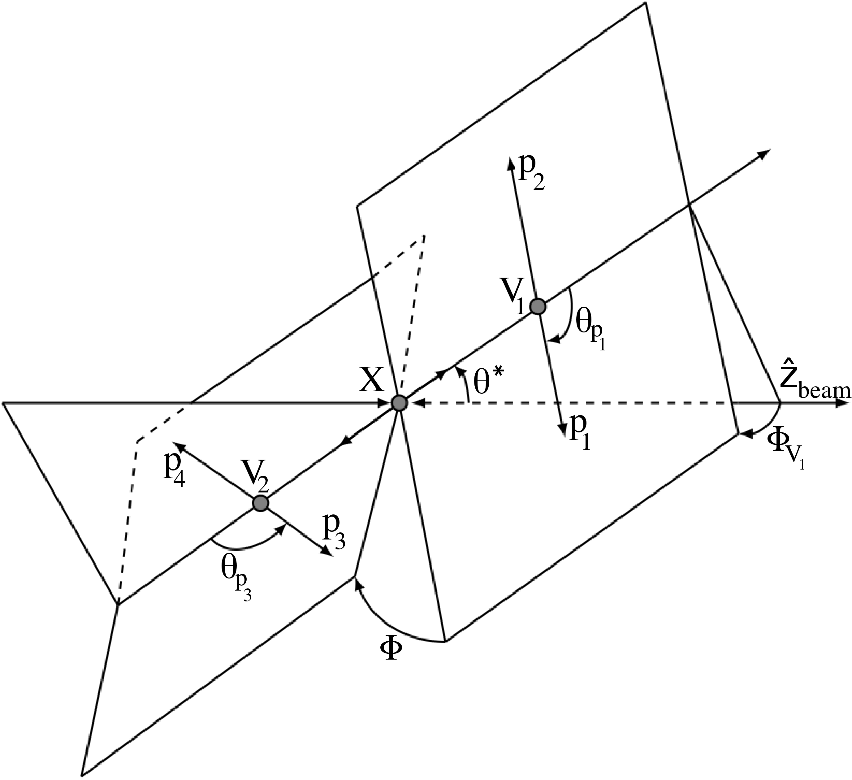
Figure 1: Representation of the Cabibbo–Maksymowicz–Dell’Aquila–Nelson angles defined in Eq. 1.

Resonances with different spins will produce different angular correlations among the decay products. A full set of analytic expressions for different resonance hypotheses and the subsequent angular correlations in the $X\to V_{1}V_{2}\to$ 4 fermion final state can be found in Ref. Bolognesi et al. (2012), which we do not reproduce here. We have verified the analytic expressions in Ref. Bolognesi et al. (2012) by comparing to parton level Monte Carlo results for different resonant spin hypotheses. Our full discussion of Monte Carlo signal samples and analysis of angular correlations analysis is given in Section III.

II.2 Phenomenology of jet substructure

While the angles defined in Fig. 1 underpin any analysis aimed at spin characterization of a given resonance, the corresponding differential distributions are expected to be smeared and skewed after accounting for showering and hadronization, detector resolution effects, jet clustering methods, and jet substructure cuts. Of these effects, the distortions introduced by jet clustering methods and jet substructure cuts are the most pernicious.

The usual goal for jet substructure techniques is to isolate the partonic constituents of a given wide angle jet that captures the decay products of a boosted parent, like a $W$, $Z$, $h$, or $t$ resonance. As a result, different methods have been developed to maximize the tagging efficiency of these parent particles while simultaneously minimizing the mistag rate from QCD or other backgrounds Altheimer et al. (2012, 2014). In this endeavor, angular observables have played an implicit role to help improve the overall tagging efficiency of a given parent particle over the QCD background, but on the other hand, recovering the full phase space of resonance decay products will be key for post-discovery signal discrimination. Moreover, understanding how angular observables are distorted by jet substructure cuts is also necessary to optimize signal hypothesis testing in a post-discovery scenario.

To this end, we review the main jet substructure methods to extract subjets from fat jets, as well as jet substructure techniques used for background discrimination. Variants of these methods are all used, as we will see, in the most recent ATLAS and CMS 8 TeV and 13 TeV analyses Aad et al. (2015a); Khachatryan et al. (2014a); ATL (2015a); CMS (2015).

Mass-drop filter technique

The jet grooming procedure used in the 8 TeV ATLAS analysis Aad et al. (2015a) is known as mass-drop filtering Butterworth et al. (2008). An original fat jet, reconstructed with the Cambridge-Aachen (C/A) cluster algorithm Dokshitzer et al. (1997), is “unclustered” in reverse order. Each step of the unclustering gives a pair of subjets that is tested for both mass-drop and momentum balance conditions. The procedure is stopped if the two conditions are satisfied.

The mass-drop criterion requires each subjet to satisfy $\mu_{i}\equiv m_{i}/m_{0}\leq\mu_{f}$ for a given parameter $\mu_{f}$, where $m_{i}$ is the subjet mass and $m_{0}$ is the original jet mass. The 8 TeV ATLAS hadronic and semi-leptonic diboson searches use $\mu_{f}=1$, which effectively means no mass-drop cut is applied.

The subjet momentum balance condition imposes a minimum threshold on the relative $p_{T}$ and $\Delta R$ of each subjet, according to

$$\sqrt{y}=\text{ min}(p_{T_{1}},\ p_{T_{2}})\frac{\Delta R}{m_{0}}\geq\sqrt{y_{\text{min}}}\ ,$$ (3)

where $p_{T_{i}}$ is the transverse momentum of each subjet $j_{i}$, $\Delta R=\sqrt{\left(\Delta\phi\right)^{2}+\left(\Delta\eta\right)^{2}}$ is their angular distance, and $\sqrt{y_{\text{min}}}$ is a parameter controlling the threshold. To see how Eq. (3) acts as a cut on the subjet momentum balance, we rewrite Eq. (3) using

$$m_{0}^{2}=2p_{T_{1}}p_{T_{2}}\left(\cosh(\Delta\eta)-\cos(\Delta\phi)\right)\approx p_{T_{1}}p_{T_{2}}(\Delta R)^{2}\ ,$$ (4)

which holds as long as the rapidity difference $\Delta\eta$ and azimuthal separation $\Delta\phi$ are small. Using this approximation, we see that the $\sqrt{y_{\text{min}}}$ cut is indeed a subjet momentum balance cut as advertised,

$$y\approx\frac{\left\{\text{ min}(p_{T_{1}},\ p_{T_{2}})\right\}^{2}}{p_{T_{1}}p_{T_{2}}}=\frac{p_{T,\text{ min}}}{p_{T,\text{ max}}}\geq y_{\text{min}}\ .$$ (5)

At each stage of the unclustering, if the pair of subjets under consideration satisfies $\sqrt{y}\geq\sqrt{y_{\text{min}}}$, the procedure terminates and the total four-momentum of the subjets are used as the $W$ or $Z$ boson candidate. If the subjets fail the cut, the softer subjet is discarded and the unclustering procedure continues.

Pruning

In contrast to mass-drop filtering, which recursively compares subjets to the original fat jet kinematics, the jet pruning method Ellis et al. (2009, 2010), which is used in the 8 TeV CMS analysis Khachatryan et al. (2014a), tests each stage of the reclustering for sufficient hardness and discards soft recombinations. In this way, each stage of the reclustering offers an opportunity to remove constituents from the final jet, instead of simply incorporating the soft contamination into the widest subjets.

Concretely, in the jet pruning method, the constituents of a fat jet are reclustered using the C/A algorithm if they are sufficiently balanced in transverse momentum and sufficiently close in $\Delta R$. The transverse momentum balance condition is dictated by a minimum requirement on the hardness $z$, defined by

$$z=\text{ min}\left(\frac{p_{T_{i}}}{p_{T_{p}}},\frac{p_{T_{j}}}{p_{T_{p}}}\right)\ ,$$ (6)

where $p_{T_{p}}$ is the sum of the tranverse momentum of the psuedojets $i$ and $j$. Note that $z$ is related the momentum fraction $y$ from Eq. (5) via

$$y\approx\frac{p_{T,\text{ min}}}{p_{T,\text{ max}}}=\frac{z}{1-z}\ .$$ (7)

In addition to having sufficient hardness, the two pseudojets must also be closer in $\Delta R$ than a parameter $D_{\text{cut}}$, given by

$$\Delta R_{ij}>D_{\text{cut}}\equiv\frac{m_{\text{orig}}}{p_{T,\text{ orig}}}\ ,$$ (8)

where $m_{\text{orig}}$ and $p_{T,\text{ orig}}$ are the invariant mass and transverse momentum of the original fat jet. If either the hardness or the $\Delta R$ cut fails, then the softer $p_{T}$ pseudojet is discarded. The C/A reclustering procedure continues until all the constituents of the original fat jet are included or discarded.

$N$-subjettiness

The $N$-subjettiness variable Thaler and Van Tilburg (2011, 2012) is used by CMS in their 8 TeV and 13 TeV analyses Khachatryan et al. (2014a); CMS (2015) to help suppress QCD multi-jet backgrounds and improve selection of hadronic $W$ and $Z$ candidates. The $N$-subjettiness is defined as

$$\tau_{N}=\frac{1}{d_{0}}\sum\limits_{k}p_{T_{k}}\text{ min}(\Delta R_{1,k},\ldots,\Delta R_{N,k})\ ,$$ (9)

where $p_{T_{k}}$ is the transverse momentum of the $k$th constituent of the original jet and $\Delta R_{n,k}$ is the angular distance to the $n$th subjet axis. The set of $N$ subjets is determined by reclustering all jet constituents of the unpruned jet with the $k_{T}$ algorithm and halting the reclustering when $N$ distinguishable pseudojets are formed. Here, $d_{0}\equiv\sum_{k}p_{T_{k}}R_{0}$ is a normalization factor for $\tau_{N}$, where $R_{0}$ is the cone size of the original fat jet. For the boosted hadronic $W$ and $Z$ analyses, the ratio $\tau_{21}=\tau_{2}/\tau_{1}$ is computed, where the signal $W$ and $Z$ candidates tend toward lower $\tau_{21}$ values, whereas the QCD background peaks at higher values.

Trimming

The 13 TeV ATLAS analysis ATL (2015a) was reoptimized for multi-TeV scale diboson sensitivity and adopts the trimming procedure Krohn et al. (2010) instead of the earlier mass-drop filtering technique. Trimming takes a large radius fat jet and reclusters the constituents with the $k_{T}$ cluster algorithm Catani et al. (1993) using distance parameter $R=0.2$. Of the resulting set of subjets, those kept must satisfy

$$\frac{p_{T_{j}}}{p_{T_{J}}}>z_{\text{min}}\ ,$$ (10)

where $j$ denotes the subjet and $J$ the original fat jet. The four-momentum sum of all remaining subjets is used as a $W$ or $Z$ candidate. For an ideal $W$ or $Z$ decay, with exactly two final subjets, the above condition translate directly to the same balance criteria as the filtering technique,

$$y\approx\frac{p_{T,\text{ min}}}{p_{T,\text{ max}}}\geq y_{\text{min}}=\frac{z_{\text{min}}}{1-z_{\text{min}}}\ .$$ (11)

Note, however, that this algorithm does not consider pairs of subjets as the pruning or filtering techniques do. Thus, it is possible to obtain more than two subjets and hence additional cuts, such as energy correlation function cuts, are needed to determine whether the trimmed jet has a two-prong substructure.

Energy Correlation Functions

The ATLAS 13 TeV analysis ATL (2015a) uses energy correlation functions Larkoski et al. (2013, 2014, 2015) to characterize the number of hard subjets in their set of trimmed jets. The relevant 1-point, 2-point and 3-point energy correlation functions are

$$e_{1}^{(\beta)} =\sum\limits_{1\leq i\leq n_{J}}p_{T_{i}}\ ,$$

$$e_{2}^{(\beta)} =\sum\limits_{1\leq i<j\leq n_{J}}p_{T_{i}}p_{T_{j}}\Delta R_{ij}^{\beta}\ ,$$

$$e_{3}^{(\beta)} =\sum\limits_{1\leq i<j<k\leq n_{J}}p_{T_{i}}p_{T_{j}}p_{T_{k}}\Delta R_{ij}^{\beta}\Delta R_{ik}^{\beta}\Delta R_{jk}^{\beta}\ ,$$ (12)

where the sums are performed over jet constituents and $\beta$ is a parameter weighting the angular separations of constituents against their $p_{T}$ fractions. Since the sums are performed over jet constituents, the energy correlation functions are independent of any jet algorithm. An upper limit is set on the ratio of the function

$$D_{2}^{(\beta)}=\frac{e_{3}^{(\beta)}\left(e_{1}^{(\beta)}\right)^{3}}{\left(e_{2}^{(\beta)}\right)^{3}}\ ,$$ (13)

where the ATLAS collaboration uses $\beta=1$ in their 13 TeV analysis.

III Angular observables in the $4q$ final state: the 2 TeV case study

III.1 Signal benchmarks

We consider spin-0, spin-1 $W^{\prime}$, spin-1 $Z^{\prime}$, spin-1 $W_{R}$, and spin-2 new physics resonances as possible candidates for the 2 TeV excess from the ATLAS 8 TeV analysis Aad et al. (2015a). The spin-0 possibility is an ad-hoc real scalar model built from the Universal FeynRules Output Alloul et al. (2014) implementation of the SM Higgs effective couplings to gluons in MadGraph v.1.5.14 Alwall et al. (2011), and is included only as an example of a heavy real scalar that couples dominantly to longitudinal vector bosons. The spin-1 $W^{\prime}$ and spin-1 $Z^{\prime}$ possibilities are based on the Heavy Vector Triplet model Pappadopulo et al. (2014); Thamm et al. (2015), whose phenomenology related to the ATLAS 2 TeV diboson excess was described in detail in Ref. Thamm et al. (2015). The spin-1 $W_{R}$ explanation is taken from the UFO model files that accompany Ref. Dobrescu and Fox (2015). The spin-2 heavy graviton resonance is adapted from a Randall-Sundrum scenario Randall and Sundrum (1999a, b) as a MadGraph model file implementation Hagiwara et al. (2008).

Each of these signal possibilities is generated as an on-shell resonance in MadGraph with subsequent decays to massive electroweak diboson and then final state SM fermions. These parton level events are then showered and hadronized with Pythia v.8.2 Sjöstrand et al. (2015), processed through Delphes v.3.1 de Favereau et al. (2014) for detector simulation, and clustered into jets using the FastJet v.3.1.0 Cacciari et al. (2012) as each ATLAS or CMS analysis requires. Because Delphes does not include parametrized detector simulation of jet constituents, which are the basis for studying jet substructure and angular correlations between subjets, we also post-process the jet constituents to smear their $p_{T}$, $\phi$, and $\eta$ to mimic detector resolution effects: the constituent smearing parameters are rescaled by the respective energy fraction of the constituent compared to the full jet.

We simulate QCD dijet background with Pythia v.8.2 Sjöstrand et al. (2015). The subsequent event evolution is the same as described above.

III.2 ATLAS and CMS analysis cuts at 8 TeV and 13 TeV

We recast the ATLAS and CMS searches for heavy resonances with hadronic diboson decays at 8 TeV Aad et al. (2015a); Khachatryan et al. (2014a) and 13 TeV ATL (2015a); CMS (2015). As the angular correlations in term of the parameterization of Sec. II are skewed by the actual analyses, we briefly summarize the basic selection criteria for the different searches.

$4q$ Final State by ATLAS at 8 TeV

In the fully hadronic ATLAS search for diboson resonances at 8 TeV, jets are clustered with the C/A algorithm with radius $R=1.2$, and events must have two jets with $p_{T}>20$ GeV and $|\eta|<2.0$. If there are electrons with $E_{T}>20$ GeV and $|\eta|<1.37$ or $1.52<|\eta|<2.47$, or if there are muons with $p_{T}>20$ GeV and $|\eta|<2.5$, the event is vetoed. Events must also have $\not{E}_{T}<350$ GeV.

The two fat jets are then filtered with $y_{\text{min}}=0.04$. The constituents of the two subjets of the groomed jet are then reclustered again with the C/A algorithm but with a smaller cone size of $R=0.3$. The up to three highest-$p_{T}$ jets, which we will call filtered jets, are used to reconstruct the $W$ or $Z$ boson candidate. Having reconstructed the ungroomed, groomed, and filtered jets, further event selection cuts are applied. The rapidity difference between the ungroomed jets must satisfy $|y_{J_{1}}-y_{J_{2}}|<1.2$. Additionally, the $p_{T}$ asymmetry of ungroomed jets must be small, $\left(p_{T,\ J_{1}}-p_{T,\ J_{2}}\right)/\left(p_{T,\ J_{1}}+p_{T,\ J_{2}}\right)<0.15$. The ungroomed and corresponding groomed and filtered jets are tagged as a $W$ or $Z$ boson if they fulfill the following three criteria:

• The pair of subjets of the groomed jet must satisfy a stronger transverse momentum balance requirement, $y\geq y_{\text{min}}=0.2025$.

• The number of charged tracks associated to the ungroomed jet has to be less than $n_{\text{trk}}<30$. Only well-reconstructed tracks with $p_{T}\geq 500$ MeV are used.

• The $W$ or $Z$ boson candidates, reconstructed from the filtered jets, are finally tagged as a $W$ and/or $Z$, if their invariant mass fulfills $|m_{J}-m_{V}|<13$ GeV. Here, $m_{V}$ is either 82.4 GeV for a $W$ boson or 92.8 GeV for a $Z$ boson, as determined ATLAS full simulation.

Finally, the event is required to have the two highest-$p_{T}$ jets be boson-tagged and $m_{JJ}>1.05$ TeV.

$4q$ Final State by CMS at 8 TeV

The CMS 8 TeV analysis uses jet pruning to reconstruct a diboson resonance. Jets are reconstructed with the C/A algorithm using $R=0.8$, and events must have at least two jets with $p_{T}>30$ GeV and $|\eta|<2.5$, where the two leading jets must satisfy $|\Delta\eta|<1.3$ and $m_{JJ}>890$ GeV. The two jets are pruned with $z_{\text{min}}=0.1$ (roughly equivalent to $y_{\text{min}}=0.11$) and the corresponding $W$/$Z$ candidate must satisfy $70$ GeV $<m_{J}<$ 100 GeV. Jets are further categorized according to their purity using the $N$-subjettiness ratio $\tau_{21}$, where high-purity $W$/$Z$ candidates have $\tau_{21}<0.5$ and low-purity $W$/$Z$ candidates have $0.5<\tau_{21}<0.75$. The diboson resonance search requires at least one high-purity $W$/$Z$ jet, and the second $W$/$Z$ can be either high- or low-purity.

$4q$ Final State by ATLAS at 13 TeV

In ATLAS 13 TeV analysis, events are again vetoed if they contain electrons or muons with $p_{T}>25$ GeV and $|\eta|<2.5$, and events must have $\not{E}_{T}<250$ GeV. In contrast to earlier, though, jets are now clustered using the anti-$k_{T}$ cluster algorithm Cacciari et al. (2008) with $R=1.0$, and events must have two fat jets with $p_{T}>200$ GeV, $|\eta|<2.0$ and $m_{J}>50$ GeV. The leading jet must have $p_{T}>450$ GeV, the invariant mass of the two fat jets must lie between 1 TeV and 2.5 TeV, and the rapidity separation must be small, $|y_{J_{1}}-y_{J_{2}}|<1.2$. Furthermore, the leading two jets must also have a small $p_{T}$ asymmetry, $\left(p_{T,\ J_{1}}-p_{T,\ J_{2}}\right)/\left(p_{T,\ J_{1}}+p_{T,\ J_{2}}\right)<0.15$.

Jets are then trimmed, instead of filtered, by reclustering with the $k_{T}$ algorithm using $R=0.2$ and using hardness parameter $z_{\text{min}}=0.05$, and the energy correlation functions for $D_{2}^{(\beta=1)}$ are then calculated on the trimmed jets to help distinguish $W$ bosons, $Z$ bosons, and multijet background. The upper limit on $D_{2}$ varies for $W$ and $Z$ candidates as well as the $p_{T}$ of the trimmed jet: to implement this $D_{2}$ cut, we linearly interpolate between the two cut values, $D_{2}=1.0$ at $p_{T}=250$ GeV and $D_{2}=1.8$ at $p_{T}=1500$ GeV, quoted in their analysis. The trimmed jets are tagged as bosons if they fulfill two final criteria: $N_{\text{trk}}<30$ for charged-particle tracks associated with the ungroomed jet and $|m_{J}-m_{V}|<15$ GeV, where $m_{V}=84$ GeV for a $W$ boson and $m_{V}=96$ GeV for a $Z$ boson.

$4q$ Final State by CMS at 13 TeV

The CMS 13 TeV analysis shares many of the same selection criteria as their 8 TeV analysis, with the following adjustments. The two anti-$k_{T}$, $R=0.8$, $p_{T}>30$ GeV jets must now lie within $|\eta|<2.4$. The pseudorapidity separation between the two jets must again satisfy $|\Delta\eta|<1.3$, and the minimum invariant mass cut on $m_{JJ}$ is raised to 1 TeV. The two jets are again pruned with $z_{\text{min}}=0.1$ and the pruned jet mass window is widened, allowing 65 GeV$<m_{W/Z}<$ 105 GeV. Finally, the $N$-subjettiness ratio $\tau_{21}$ is again calculated, where high-purity $W/Z$ jets must have a slightly harder requirement, $\tau_{21}\leq 0.45$, and low-purity $W/Z$ jets satisfy $0.45<\tau_{21}<0.75$. The event must have at least one high-purity $W/Z$ jet and is classified as high-purity or low-purity according to the second jet.

III.3 Analysis effects and reconstruction

We implement the fully hadronic ATLAS and CMS diboson searches on the signal samples presented in Sec. III.1, and we extract the angular observables reviewed in Sec. II.1 from the subjets of the reconstructed $W/Z$-tagged boson. Since $W/Z$ discrimination is very difficult in this final state, we merge the $\cos\theta_{p_{1}}$ and $\cos\theta_{p_{3}}$ distributions into a single differential distribution labeled $\cos\theta_{q}$ and do not differentiate between $W$ and $Z$ candidates. We also recognize that these analyses do not attempt to distinguish quarks from anti-quarks, hence we randomly assign the $p_{1}$ and $p_{2}$ labels (or $p_{3}$ and $p_{4}$ labels) to subjets of a given $W/Z$ candidate, which renders the signs of different angles ambiguous. Finally, we merge the high-purity and low-purity tagged events in the CMS analyses to ensure our angular sensitivity analysis has reasonable statistics.

We find that of the angles defined in Sec. II, the main discrimination power between different spin scearios comes from $\cos{\theta^{*}}$, $\cos{\theta_{q}}$ and $\Psi$. In the remainder of this Section, we will present the individual differential shapes for the different Monte Carlo samples and experimental studies, and explain how they are skewed by the respective event selection and jet substructure cuts. All of our figures show both parton and reconstruction level unit-normalized distributions for the different signal samples and QCD multijet background, where all showering, hadronization, detector resolution, jet reconstruction, and substructure analysis effects have been included in the reconstructed differential distributions.

Differential Shape of $\cos{\theta^{*}}$

We first show the angular observable $\cos{\theta^{*}}$ in Fig. 2 for various spin-0, spin-1, and spin-2 signal benchmarks and the QCD background after implementing the ATLAS 8 TeV (upper left), CMS 8 TeV (upper right), ATLAS 13 TeV (lower left), and CMS 13 TeV (lower right) analyses. This angle measures the alignment of the vector bosons from $X$ decay with the beam axis, if we use the threshold approximation to identify the $X$ rest frame with the lab frame. We see significant discrimination power at parton level (thin lines) between the different signal benchmarks, especially between the spin-0 and spin-2 signals compared to the spin-1 benchmark. The extra oscillations in the spin-2 signal, however, are lost when comparing the reconstruction level (thick lines) distributions, leaving only the overal concavity of the spin-1 distribution the main discriminant from the spin-0, spin-2, and QCD background shapes. Comparing parton level to reconstruction level results for each signal sample, we see the experimental analyses cause significant hard cuts in $\cos{\theta^{*}}$, effectively requiring $|\cos{\theta^{*}}|\lesssim 0.55$ for ATLAS and $|\cos{\theta^{*}}|\lesssim 0.6$ for CMS, and we also see a deficit of events around $\cos{\theta^{*}}\approx 0$ is induced by each analysis, most notably in the ATLAS 13 TeV analysis.

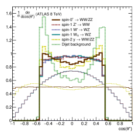
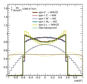
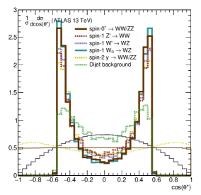
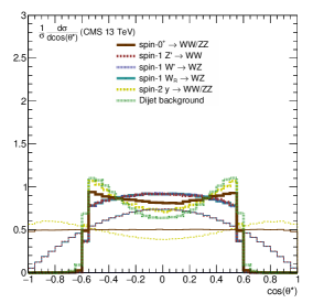
Figure 2: Comparison of the $\cos{\theta^{*}}$ angle between MC parton level results (thin lines) and reconstruction of showered events via jet substructure (thick lines) for the ATLAS (left) and CMS (right) hadronic diboson search at 8 TeV (top) and 13 TeV (bottom). Each distribution is unit-normalized.

We can identify the sharp cliffs in the $|\cos{\theta^{*}}|$ distribution with the cut on the maximum pseudorapidity difference $|\Delta\eta|$ between the two fat jets, since the $\theta^{*}$ angle is directly related to the pseudorapidity via $\eta=-\log\tan(\theta/2)$. Therefore $\cos{\theta^{*}}$ can be rewritten in the $X$ rest frame as

$$|\cos{\theta^{*}}|=\cos\left(2\arctan e^{-\frac{|\Delta\eta|}{2}}\right)=\tanh{\frac{|\Delta\eta|}{2}}\leq\tanh{\frac{|\Delta\eta_{\text{max}}|}{2}}\ .$$ (14)

Given $|\Delta y_{\text{max}}|=1.2$ at ATLAS and $|\Delta\eta_{\text{max}}|=1.3$ at CMS, and since differences in pseudorapidity are invariant under longitudinal boosts, we therefore expect sharp cuts at $|\cos{\theta^{*}}|\approx 0.54$ and $0.57$, respectively, where the steepness of the cliff is only spoiled by the net transverse momentum of the $X$ resonance in the lab frame.

The deficit of events around $\cos{\theta^{*}}\approx 0$ is a direct result of the angular scale chosen for the jet substructure analysis, where a larger angular scale causes a stronger sculpting behavior around $\cos{\theta^{*}}\approx 0$. We know from Eq. 14 that small $\cos{\theta^{*}}$ is identified with small $\Delta\eta$ between the two fat jets, and we also show in Fig. 3 the parton level correlation between $\Delta\eta$ for the two fat jets and $\Delta R$ of the resulting $W$ and $Z$ decay products for a spin-1 $W^{\prime}$ example. Other signal samples would show a similar correlation, albeit with only one $W$ (left color band) or $Z$ (right color band) as appropriate. The bulk of the $W/Z$ subjets lie at $\Delta R\approx 2m_{W/Z}/(1~{}\text{TeV})$ as expected, where 1 TeV is a rough estimate of the $W$ and $Z$ transverse momenta when the vector bosons are central, but we also see a clear correlation between larger $\Delta\eta$ separation between the fat jets and the corresponding $\Delta R$ of the resulting subjets. As $\Delta\eta$ grows, the vector bosons from the $W^{\prime}$ decay become more forward, and thus the corresponding $p_{T}$ of each vector boson decreases, leading to larger $\Delta R$ separation of their subjets.

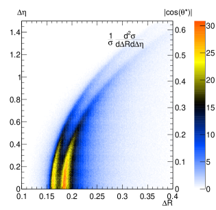
Figure 3: Spin-1 $W^{\prime}$ parton level correlation of the angular separation $\Delta R$ between the $W/Z$ decay products and the rapidity difference $\Delta\eta$ of the two $W^{\prime}\to WZ$ fat jets, where the left band shows the $W$ decay products and the right band shows the $Z$ decay products, and the shading shows the relative event weight. This correlation holds also for other spin scenarios. The $\Delta\eta$ axis is translated to a $|\cos{\theta^{*}}|$ axis according to Eq. 14.

As a result of this correlation, using a large fixed angular scale during jet substructure reclustering leads to a deficit of events with small $\Delta\eta$ separation between fat jets and hence leads to the sculpting effect around $\cos\theta^{*}\approx 0$ observed in Fig. 2. A relatively large angular scale for subjet clustering will merge nearby partons together, and the resulting event will not have the requisite subjets to define the $\cos\theta^{*}$ angle and fail the reconstruction of angular observables. The ATLAS 13 TeV analysis has the most pronounced deficit of events around $\cos\theta^{*}\approx 0$, since this analysis uses a fixed radius of $R=0.2$ during trimming. Most notably, using an angular scale of $R=0.2$ during subjet clustering causes most of the quarks to merge into a single subjet, which severely limits the viability of such a subjet identification technique for a post-discovery study of angular correlations. We remark that the $D_{2}^{(\beta=1)}$ discriminant also used in the ATLAS 13 TeV analysis to identify a prevalence of two-prong energy correlations compared to one-prong and three-prong energy correlations fails to ameliorate the situation, as the events with the strongest two-prong behavior would still need to be reclustered to identify the appropriate subjets for angular observable studies.

Differential Shape of $\cos{\theta_{q}}$

The second main discriminant between different spin signal hypotheses is the $\cos{\theta_{q}}$ angle, shown in Fig. 4, which combines the $\cos{\theta_{p_{1}}}$ and $\cos{\theta_{p_{3}}}$ angles defined in Sec. II. This angle measures the alignment of the outgoing quark with the boost vector of its parent vector in the parent rest frame, and since each event has two vector candidates, each event contribues twice to the distribution. Again we first focus on the parton level results (thin lines), which show that the spin-2 RS graviton hypothesis has the opposite concavity to the spin-0 and spin-1 signals. We note that the spin-2 resonance dominantly couples to tranversely polarized electroweak bosons, while the spin-0 and spin-1 resonances dominantly couple to longitudinal bosons. Hence, the pronounced difference in shape between the signals is a realistic proxy for studying the sensitivity of different jet substructure analyses to the polarization of $W$ and $Z$ bosons. For longitudinal bosons, the expected analytic shape of the $\cos\theta_{q}$ distribution is $\dfrac{3}{4}\left(1-\cos^{2}\theta_{q}\right)$, while the shape is $\dfrac{3}{8}\left(1+\cos^{2}\theta_{q}\right)$ for transverse bosons Bolognesi et al. (2012). We remark that enhancing sensitivity to either the center or edges of the $\cos\theta_{q}$ distribution will emphasize sensitivity to longitudinal or transverse gauge bosons, respectively. These results also agree with an earlier analysis by CMS Khachatryan et al. (2014c), but we carry the analysis further by studying multiple state-of-the-art jet substructure techniques to understand the impact of vector boson polarization on the resulting reconstruction efficiency.

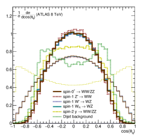
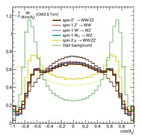
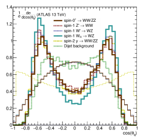
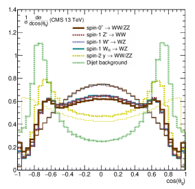
Figure 4: Comparison of the $\cos{\theta_{q}}$ angle between MC parton level results (thin lines) and reconstruction of showered events via jet substructure (thick lines) for the ATLAS (left) and CMS (right) hadronic diboson search at 8 TeV (top) and 13 TeV (bottom).

Turning to the reconstructed angular distributions (thick lines) in Fig. 4, we again see the full phase space of the parton decays gets significantly molded by the experimental analyses, where events close to $\cos{\theta_{q}}\approx\pm 1$ are cut away. In contrast to the sharp cliffs in $\cos{\theta^{*}}$, though, the $\cos{\theta_{q}}$ distribution exhibits a milder transformation, and start and strength of the deviations depend strongly on the individual analysis. At 8 TeV, ATLAS shows a reversal point at $\cos{\theta_{q}}\approx\pm 0.6$, whereas the CMS reversal point is $\cos{\theta_{q}}\approx\pm 0.8$. We also observe a deficit of events with $\cos{\theta_{q}}\approx 0$, most notably in the ATLAS 13 TeV analysis.

In order to understand the behavior around $\cos{\theta_{q}}\approx\pm 1$, we derive an approximate relation between $\cos{\theta_{q}}$ and the subjet $p_{T}$ ratio $y$. Identifying $\cos{\theta_{q}}$ with $\cos{\theta_{p_{1}}}$ for the moment, we write $\cos{\theta_{q}}\equiv\hat{p}_{p_{1}}\cdot\hat{p}_{V_{2}}$ from Eq. 1, where the $p_{1}$ and $V_{2}$ four-momenta are boosted to the $V_{1}$ rest frame. If we assume threshold production of $X$, then the $X$ rest frame is identified with the lab frame, and the two vectors $V_{1}$ and $V_{2}$ are completely back-to-back in both frames. Hence, $\hat{p}_{V_{2}}$ in the $V_{1}$ rest frame can be replaced by the (negative) boost direction $-\hat{p}_{V_{1}}$ going from the lab frame to the $V_{1}$ rest frame. If we now take the limiting case that $V_{1}$ and $V_{2}$ have no longitudinal momentum, then we are left with six four-momentum components of $p_{1}$ and $p_{2}$, which are the decay products of $V_{1}$, subject to four constraints: $(p_{1}+p_{2})^{2}=m_{V_{1}}^{2}$, $p_{1}^{2}=p_{2}^{2}=0$, and $y=p_{T_{2}}/p_{T_{1}}$ given by the $y_{\text{min}}$ cut parameter. We choose the two remaining free parameters to be the transverse momentum of the boson, $p_{T,\ V_{1}}$ and the angle between the decay plane spanned by $p_{1}$ and $p_{2}$ relative to the transverse plane. We have three planes: the plane spanned by the beam axis and the $V_{1}$ boson, the transverse plane, and the decay plane spanned by $p_{1}$ and $p_{2}$, where the common axis of intersection is the $V_{1}$ transverse momentum vector.

For the limiting case that the decay plane spanned by $p_{1}$ and $p_{2}$ aligns with the transverse plane, the cut on $y$ provides a lower bound on $|\cos\theta_{q}|$, while the case when the decay plane aligns with the plane spanned by the beam axis and the $V_{1}$ boson provides an upper bound on $|\cos\theta_{q}|$, where we can only bound $|\cos\theta_{q}|$ because we order the two subjets in $p_{T}$. These lower and upper limits are

$$\frac{p_{T,\ V}}{\sqrt{m_{V}^{2}+p_{T,\ V}^{2}}}\frac{1-y}{1+y}\leq|\cos{\theta_{q}}|\leq\frac{\sqrt{m_{V}^{2}+p_{T,\ V}^{2}}}{p_{T,\ V}}\frac{1-y}{1+y}\ .$$ (15)

Note that the upper bound can in principle exceed $1$, and at this point, for a given $p_{T,\ V}$ and $y$, the solution with the decay plane aligned with the beam axis becomes unphysical and a rotation of the decay plane away from the beam axis is needed to obtain a physical solution. If we relax the initial conditions and allow longitudinal boosts of the system, the resulting $y$ cut will, by construction, project out only the transverse components of the boost needed to transform the lab frame into the rest frame of $V_{1}$. This smears the expression in Eq. 15 for both the upper and lower limits.

Nevertheless, we can see that in the limit $p_{T,\ V}\gg m_{V}$,

$$|\cos{\theta_{q}}|\approx\frac{1-y}{1+y}\leq\frac{1-y_{\text{min}}}{1+y_{\text{min}}}\ .$$ (16)

For $y_{\text{min}}=0.20$, $0.11$, or $0.05$ for the ATLAS 8 TeV, CMS, and ATLAS 13 TeV analyses, respectively, we expect edges in the $|\cos{\theta_{q}}|$ distribution at approximately $0.66$, $0.80$, and $0.90$. As mentioned before, the analytic calculation above requires assumptions about the necessary boost to move from the lab frame to the $V_{1}$ rest frame and taking $p_{T,\ V}\gg m_{V}$, and if these assumptions are violated, the upper limit on $|\cos{\theta_{q}}|$ can be exceeded.

This discussion explains the results in Fig. 4, except for the ATLAS 13 TeV analysis, where many more events are lost then simply those beyond the derived edge at $|\cos{\theta_{q}}|=0.9$. This is because the ATLAS 13 TeV imposes an effectively tighter $y_{\text{min}}$ criteria via the $D_{2}^{(\beta=1)}$ discriminant, which we demonstrate in Fig. 5. We see that an event with a low subjet $p_{T}$ ratio would generally have a large value of $D_{2}^{(\beta=1)}$ and thus be removed given the $D_{2}$ cut. As a reminder, the $D_{2}$ cut parameter varies from $D_{2}=1.0$ for a trimmed jet of $p_{T}=250$ GeV to $D_{2}=1.8$ for $p_{T}=1500$ GeV, which corresponds to $y_{\text{min}}\approx 0.1$–$0.2$, in agreement with the resulting sculpting seen in Fig. 4.

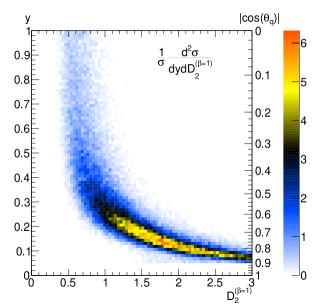
Figure 5: Correlation between the energy correlation function $D_{2}^{(\beta=1)}$ and the ratio of transverse momentum $y$ of the two leading subjets, where the shading shows the relative event weight. All analysis cuts of the ATLAS 13 TeV analysis are applied, except the cut on $D_{2}^{(\beta=1)}$ itself. This particular plot is based on the spin-1 $W^{\prime}$ model, but the correlation seen holds also for other spin scenarios. The $y$ axis is translated to a $|\cos{\theta_{q}}|$ axis according to Eq. 16.

Finally, the deficit of events with $\cos{\theta_{q}}\approx 0$ is the same sculpting effect as seen before around $\cos{\theta^{*}}\approx 0$. In Fig. 6, we show the correlation between $\Delta R$ of the $W$/$Z$ decays and the ratio of quark transverse momentum $y$ for parton-level $W^{\prime}\to WZ$ events. As before, the left band shows the $W^{\pm}$ daughter partons and the right band shows the $Z$ daughter quarks. Since using a large $\Delta R$ during subjet finding causes the $W$/$Z$ decay partons to be merged, events with large $y$ are more likely to be removed from the event sample by subsequent kinematic cuts. Using Eq. 16, we can relate $y$ to an effective cut on $\cos{\theta_{q}}$, which explains the deficit of events seen around $\cos{\theta_{q}}\approx 0$ in Fig. 4, most notably in the lower left panel for the ATLAS 13 TeV analysis.

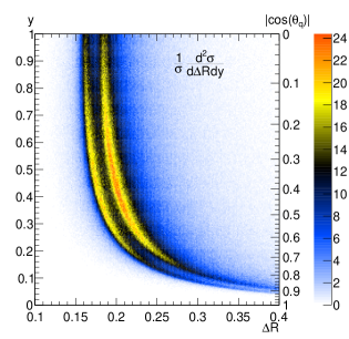
Figure 6: Spin-1 $W^{\prime}$ parton level correlations of the angular separation $\Delta R$ between the $W$/$Z$ decay products and their ratio in transverse momentum $y$, where the shading shows the relative event rate. This basic correlation holds also for other spin scenarios. The $y$ axis is translated to an approximate $|\cos{\theta_{q}}|$ axis according to Eq. 16.

Differential Shape of $\Psi$

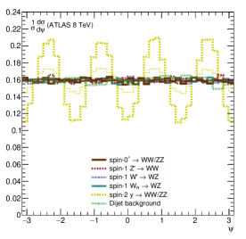
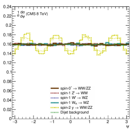
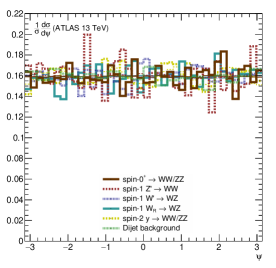
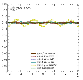
Figure 7: Comparison of the $\Psi$ angle between MC parton level results (thin lines) and reconstruction of showered events via jet substructure (thick lines) for the ATLAS (left) and CMS (right) hadronic diboson search at 8 TeV (top) and 13 TeV (bottom).

As shown in Fig. 7, the differential distribution in the angle $\Psi$ is flat for all spin hypotheses except for the spin-2 resonance. We will thus focus on explaining the behavior of the spin-2 scenario. In this distribution, we expect amplitudes proportional to $1$ and $\cos{(4\Psi)}$, where the respective amplitudes at parton level depend on the helicity states of the vector bosons and the production level partons Gao et al. (2010); Bolognesi et al. (2012). A $\cos{(2\Psi)}$ contribution would only appear when particles and anti-particles of the $V$ decay can be distinguished. Curiously, the differential distribution of $\Psi$ after cuts causes the $\cos{(4\Psi)}$ amplitude to increase. This is related to the same two cuts on $\Delta\eta_{JJ,\text{ max}}$ and subjet $p_{T}$ ratio $y_{\text{min}}$, which already skewed the $\cos{\theta^{*}}$ and $\cos{\theta_{q}}$ angle.

We can analytically determine the differential shape of the $\Psi$ distribution as a function of the cut values on $\Delta\eta_{JJ,\text{ max}}$ and $y_{\text{min}}$, using the fully differential results in Ref. Bolognesi et al. (2012). The normalized shape can be expressed as

$$\frac{1}{\sigma^{\text{(spin-2)}}}\frac{d\sigma^{\text{(spin-2)}}}{d\Psi}=\frac{1}{2\pi}-\mathcal{A}(y_{\text{min}},\Delta\eta_{\text{max}})\cos(4\Psi)\ ,$$ (17)

with

$$\mathcal{A}=\frac{1}{24\pi} F_{+-}\left(1+4y_{\text{min}}+y_{\text{min}}^{2}\right)^{2}(5f_{q\bar{q}}-1)(8+6\cosh{\Delta\eta_{\text{max}}}+\cosh{2\Delta\eta_{\text{max}}})\Big{/}$$ (18)

$$\biggl{[} F_{+-}\left(1+y_{\text{min}}+y_{\text{min}}^{2}\right)^{2}\Bigl{(}(5f_{q\bar{q}}+1)(1+2\cosh{\Delta\eta_{\text{max}}})+2\cosh{2\Delta\eta_{\text{max}}}\Bigr{)}\ +$$

$$F_{00}\left(1+4y_{\text{min}}+y_{\text{min}}^{2}\right)^{2}(-15f_{q\bar{q}}+8+6\cosh{\Delta\eta_{\text{max}}}+\cosh{2\Delta\eta_{\text{max}}})\biggr{]}\ .$$

Here, $F_{\lambda_{1}\lambda_{2}}$ is the fraction of events with two gauge bosons having a helicity $\lambda_{1}$ and $\lambda_{2}$ respectively, and $f_{q\bar{q}}$ is the production fraction from $q\bar{q}$ initial state quarks. From our Monte Carlo simulation at 8 TeV, we find $F_{+-}=F_{-+}=45.8\%$, $F_{00}=7.8\%$ and $0.6\%$ others, and thus we neglected the subleading helicity components, which are suppressed by powers of $m_{W/Z}/m_{X}$. Furthermore, we find $f_{q\bar{q}}\approx 65.5\%$ at 8 TeV LHC, while it drops to $f_{q\bar{q}}\approx 45.0\%$ at 13 TeV LHC. We show the scaling behaviour of $\mathcal{A}$ in Fig. 8.

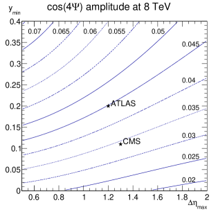
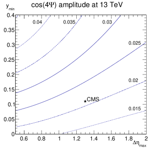
Figure 8: Expected $\cos(4\Psi)$ amplitude $\mathcal{A}$ (contours) for a spin-2 resonance at 8 TeV (left) and 13 TeV (right) as function of the cut parameter $y_{\text{min}}$ and $\Delta\eta_{JJ,\text{ max}}$, as shown in Eq. 18. We use $F_{+-}=F_{-+}=45.8\%$ and $F_{00}=7.8\%$, as determined from our underlying Monte Carlo simulation, and $f_{q\bar{q}}=65.5\%$ and $f_{q\bar{q}}=45.0\%$ for 8 TeV and 13 TeV, respectively. We also show the respective working points of ATLAS and CMS, except for ATLAS at 13 TeV, where the effective $y_{\text{min}}$ is not a fixed parameter.

From Fig. 8, we can directly read off the expected $\cos(4\Psi)$ amplitude for our 8 TeV and 13 TeV signal sample. Using $y_{\text{min}}\rightarrow 0$ and $\Delta\eta_{JJ,\text{ max}}\rightarrow\infty$ the predicted amplitudes at parton level match with $\mathcal{A}\approx 0.014$ at 8 TeV and $\mathcal{A}\approx 0.0077$ at 13 TeV very well our Monte Carlo simulation. Including cuts we expect $\mathcal{A}\approx 0.045$ and $\mathcal{A}\approx 0.034$ for ATLAS and CMS at 8 TeV, respectively, and $\mathcal{A}\approx 0.021$ for CMS at 13 TeV. For CMS the expected amplitude is slightly larger than that seen in Fig. 7, which can be explained by the approximation of Eq. 16 used to relate $\cos\theta_{q}$ with $y_{\text{min}}$.

IV Angular observables in semi-leptonic final states

We now turn to the semi-leptonic analyses, $X\to\ell\ell qq$ and $X\to\ell\nu qq$, which provide important cross-channels for a future discovery of a diboson resonance. To reiterate, the relative rates of the $4q$, $\ell\ell qq$, and $\ell\nu qq$ final states will disentangle the intermediate $W^{+}W^{-}$, $W^{\pm}Z$, and $ZZ$ nature of the resonance, which is very difficult to do using only the $4q$ analysis. Moreover, the semileptonic channels enjoy cleaner reconstruction of angular observables, larger signal efficiencies, and better control of systematic uncertainties, counterbalanced by lower overall statistical power. The importance of the semileptonic channel, especially compared to the fully leptonic channel, was emphasized, for example, in Refs. Hackstein and Spannowsky (2010); Englert et al. (2010). In particular, the angular observables $\cos\theta_{p_{1}}$ and $\cos\theta_{p_{3}}$, which were previously combined into $\cos\theta_{q}$ because we could not trace a given parent from one event to the next, are now assigned as $\cos\theta_{q}$ and $\cos\theta_{l}$. In addition, for the $\ell\nu qq$ analysis, the $\cos\theta_{l}$ distribution is asymmetric because the charge of the lepton distinguishes leptons from the anti-lepton, in constrast to the $4q$ case. We begin again by summarizing the semi-leptonic analyses by ATLAS and CMS CMS (2015); Aad et al. (2015b, c); Khachatryan et al. (2014b); ATL (2015b, c) and then present the corresponding angular distributions.

IV.1 ATLAS and CMS semi-leptonic analyses at 8 TeV and 13 TeV

$\ell\ell qq$ Final State by ATLAS at 8 TeV

In the $\ell\ell qq$ ATLAS analysis at 8 TeV, events are required to have exactly two muons of opposite charge or two electrons, where muons must have $p_{T}>25$ GeV and $|\eta|<2.4$ and electrons must have $p_{T}>25$ GeV and $|\eta|<2.47$, excluding $1.37<|\eta|<1.52$. In addition, all leptons must pass a track isolation (calorimeter isolation) requirement (see Ref. Aad et al. (2015b) for details). The lepton pair must have 66 GeV$<m_{\ell\ell}<$ 116 GeV and $p_{T}^{\ell\ell}>400$ GeV.

Jets are clustered using the C/A algorithm with $R=1.2$ and need to have $p_{T}>100$ GeV and $|\eta|<1.2$. One jet needs to survive the grooming procedure with $y_{\text{min}}=0.2025$ and fulfill $p_{T}>400$ GeV and 70 GeV$<m<$110 GeV.

$\ell\ell qq$ Final State by CMS at 8 TeV

In the CMS 8 TeV $\ell\ell qq$ analysis, electrons with $p_{T}>40$ GeV and $|\eta|<2.5$, excluding $1.44<|\eta|<1.56$, muons with $p_{T}>20$ GeV and $|\eta|<2.1$ are selected, and all leptons must be isolated from other tracks as well as in the calorimeter. Two same flavor, opposite charge, leptons are required, and for dimuon events, the leading muon must have $p_{T}>40$ GeV. The lepton pair must have 70 GeV $<m_{\ell\ell}<$ 110 GeV.

Jets are reconstructed with the C/A algorithm using $R=0.8$ and must have $p_{T}>30$ GeV and $|\eta|<2.4$. They are pruned with $z_{\text{min}}=0.1$ and are categorized by purity according the $N$-subjettiness variable $\tau_{21}$, analogous to the CMS $4q$ search. The pruned jet mass must lie within 65 GeV $<m_{J}<$ 110 GeV. Both the leptonic and hadronic vector boson candidates must have $p_{T}^{V}>80$ GeV and satisfy $m_{VV}>500$ GeV. If there are multiple hadronic $V$ candidates, the hardest $p_{T}$ candidate in the higher purity category is used.

$\ell\ell qq$ Final State by ATLAS at 13 TeV

ATLAS uses the same kinematic acceptance cuts on electrons and muons in the 13 TeV analysis as the 8 TeV analysis, and track isolation requirements are imposed. Two muons of opposite charge or two electrons are required, where the lepton pair must have 66 GeV $<m_{\mu^{+}\mu^{-}}<$ 116 GeV or 83 GeV$<m_{e^{+}e^{-}}<$ 99 GeV, respectively.

Jets are clustered using the anti-$k_{T}$ algorithm with $R=1.0$ and are required to have $p_{T}>200$ GeV and $|\eta|<2.0$. The leading jet must satisfy the trimming procedure with $z_{\text{min}}=0.05$, and fulfill $p_{T}^{J}>0.4m_{\ell\ell J}$ and $68.2\text{ GeV}<m_{J}<108.4$ GeV. Additionally, the jet needs to statisfy an upper bound on the $D_{2}^{(\beta=1)}$ energy correlator function. For simplicity, we linearly interpolate the $D_{2}$ cut between the two points quoted, $D_{2}<1.0$ at $p_{T}^{J}=250$ GeV and $D_{2}<1.8$ at $p_{T}^{J}=1500$ GeV. Finally, the dilepton system must have $p_{T}^{\ell\ell}>0.4m_{\ell\ell J}$.

$\ell\nu qq$ Final State by ATLAS at 8 TeV

In the 8 TeV ATLAS $\ell\nu qq$ analsis, the lepton kinematic criteria are the same as their 8 TeV $\ell\ell qq$ search, and a similar isolation criteria is used. Missing transverse energy $\not{E}_{T}$ (MET) must exceed $30$ GeV and is used to calculate the corresponding neutrino four-momentum assuming no other source of MET and $m_{W}^{2}=(p_{\ell}+p_{\nu})^{2}$:

$$p_{z}^{\nu}=\frac{1}{2p_{T}^{\ell}}\left[(m_{W}^{2}+2\vec{p}_{T}^{~{}\ell}\cdot\vec{p}_{T}^{~{}\nu})p_{z}^{~{}\ell}\pm E^{\ell}\sqrt{(m_{W}^{2}+2\vec{p}_{T}^{~{}\ell}\cdot\not{\vec{E}}_{T})^{2}-4(p_{T}^{~{}\ell})^{2}\not{E}_{T}^{2}}\right]\ .$$ (19)

In the case of two complex solutions for $p_{Z}^{\nu}$, the real part is used, otherwise the smaller solution in absolute value is used. Events are required to have $p_{T}^{\ell\nu}>400$ GeV.

Jets are clustered using the C/A algorithm with $R=1.2$. One jet must survive the grooming procedure with $y_{\text{min}}=0.2025$ and fulfill $p_{T}^{J}>400$ GeV, $|\eta|<2.0$ and $65\text{ GeV}<m_{J}<105$ GeV, and the $\Delta\phi$ between this jet and the MET vector must exceed 1. Events with at least one $b$-tagged jet are vetoed (see Ref. Aad et al. (2015c) for details).

$\ell\nu qq$ Final State by CMS at 8 TeV

At CMS, electrons with $p_{T}>90$ GeV and $|\eta|<2.5$, excluding $1.44<|\eta|<1.56$, and muons with $p_{T}>50$ GeV and $|\eta|<2.1$ are selected. The same isolation criteria from the CMS $\ell\ell qq$ search are applied. A single muon or electron is required and MET must exceed 40 GeV or 80 GeV, respectively. The corresponding neutrino four-momentum is reconstructed as in the ATLAS $\ell\nu qq$ search, and $p_{T}^{\ell\nu}>200$ GeV is required.

Jets are reconstructed with the C/A algorithm using $R=0.8$, $p_{T}>30$ and $|\eta|<2.4$. They are pruned with $z_{\text{min}}=0.1$ and categorized by purity using $\tau_{21}$, as in the CMS $4q$ and $\ell\ell qq$ searches. The pruned jet mass must again lie within 65 GeV $<m_{J}<$ 110 GeV and have $p_{T}^{J}>200$ GeV, and if there are multiple hadronic $V$ candidates, the hardest $p_{T}$ candidate in the higher purity category is used. Furthermore, $\Delta R_{J,\ (\ell\nu)}>\pi/2$, $\Delta\phi_{J,\ \not{E}_{T}}>2.0$, $\Delta\phi_{J,\ (\ell\nu)}>2.0$ and $m_{J\ell\nu}>700$ GeV are required. Events with one $b$-tagged jet are vetoed.

$\ell\nu qq$ Final State by ATLAS at 13 TeV

For the ATLAS 13 TeV $\ell\nu qq$ search, leptons are identified as in the ATLAS $\ell\ell qq$ final state search at 8 TeV. Events must have one lepton and $\not{E}_{T}>100$ GeV, and the neutrino four-momentum is reconstructed as in the 8 TeV analysis.

Jets are clustered using the anti-$k_{T}$ algorithm with $R=1.0$. The leading jet must survive the trimming procedure with $z_{\text{min}}=0.05$ and fulfill $p_{T}>200$ GeV, $|\eta|<2.0$, $70.2\text{ GeV}<m_{J}<106.4$ GeV, and $p_{T}^{J}>0.4m_{\ell\nu J}$. The same $D_{2}^{(\beta=1)}$ energy correlator cut as the 13 TeV $\ell\ell qq$ ATLAS search is imposed. Finally, events must have $p_{T}^{\ell\nu}>0.4m_{\ell\nu J}$ and $p_{T}^{\ell\nu}>200$ GeV, and events with $b$-tagged jets are vetoed.

$\ell\nu qq$ Final State by CMS at 13 TeV

Lastly, for the CMS $\ell\nu qq$ search at 13 TeV, events must have a single electron or muon, where electron candidates must have $p_{T}>120$ GeV and $|\eta|<2.5$, excluding $1.44<|\eta|<1.56$, and muon candidates must have $p_{T}>53$ GeV and $|\eta|<2.1$. The same lepton isolation criteria as the CMS $\ell\ell qq$ search are applied. Electron (muon) events must have at least 80 GeV (40 GeV) of MET. The neutrino four-momentum is reconstructed as in the ATLAS $\ell\nu qq$ final state search, and the lepton-neutrino system must have $p_{T}^{\ell\nu}>200$ GeV.

Jets are reconstructed with the anti-$k_{T}$ algorithm using $R=0.8$, $p_{T}>30$ GeV and $|\eta|<2.4$. They are pruned with $z_{\text{min}}=0.1$ and categorized by purity using the same criteria as the 13 TeV CMS $4q$ search. To satisfy the boson tagging requirements, a pruned jet $J$ has to fulfill $65\text{ GeV}<m_{J}<105$ GeV and $p_{T}^{J}>200$ GeV, and for events with multiple hadronic boson candidates, the highest $p_{T}$ jet with the higher purity category is used. Events must also pass $\Delta R_{J,\ (\ell\nu)}>\pi/2$, $\Delta\phi_{J,\ \not{E}_{T}}>2.0$, $\Delta\phi_{J,\ (\ell\nu)}>2.0$, and $m_{J\ell\nu}>700$ GeV cuts, and events with $b$-tagged jets are vetoed.

IV.2 Angular observables in semi-leptonic final states and comparison with fully hadronic final states

In Fig. 9, we show the normalized distributions for the $\cos\theta^{*}$, $\cos\theta_{q}$, $\cos\theta_{l}$, and $\Psi$ angles for the relevant ATLAS and CMS $\ell\ell qq$ analyses. Note that we do not show the $\ell\ell qq$ background or the parton-level results in this plots. The $\ell\ell qq$ final state mimics the $4q$ final state, since the entire $X\to\ell\ell qq$ system is in principle reconstructible. Moreover, as mentioned before, the $\cos\theta_{q}$ distribution for the $4q$ final state splits into the new $\cos\theta_{q}$ and $\cos\theta_{l}$ angles, because the final state partons are distinguishable. On the other hand, the $\ell\ell qq$ final state pays an intrinsic penalty in statistical power, since the branching ratio Br$(W^{\pm}Z\to\ell\ell qq)$ / Br$(W^{\pm}Z\to 4q)\approx 0.094$, for $\ell=e$, $\mu$, is only partially mitigated by an improved semileptonic signal efficiency. Thus, the $4q$ and semileptonic channels play important complementary roles both in the discovery of a new resonance but also give significant cross-checks for spin discrimination.

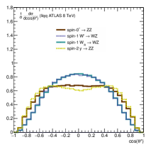
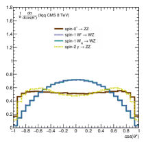
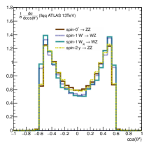
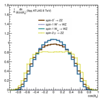
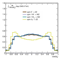
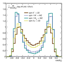
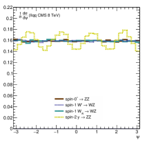
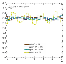
Figure 9: Normalized differential distributions for $\cos\theta^{*}$ (top row), $\cos\theta_{q}$ (second row), $\cos\theta_{l}$ (third row), and $\Psi$ (bottom row) angles in the semi-leptonic final state $\ell\ell qq$, after imposing the ATLAS 8 TeV (left column), CMS 8 TeV (middle), and ATLAS 13 TeV (right) analysis cuts.

From Fig. 9, we see that angular observables again provide important discrimination power between spin-2 and the other spin hypotheses, while the main sensitivity to distinguish spin-0 from spin-1 resonances comes from the $\cos\theta^{*}$ angle. The sculpting effects we identified earlier are still evident in $\cos\theta_{q}$ as a result of the jet substructure cuts, but on the other hand, most of the phase space is preserved for the $\cos\theta_{l}$ distribution. Note that there is no $p_{T}$ requirement on the individual subjets in contrast to the hard cut on the lepton $p_{T}$. This effectively flattens the $\cos\theta_{l}$ shape for the spin-2 resonance compared to $\cos\theta_{q}$, as events with large lepton $p_{T}$ imbalance near $\cos\theta_{l}=\pm 1$ tends to miss one of the leptons.

One interesting feature is the sharp cliff in $\cos\theta^{*}$ for the ATLAS 13 TeV analysis, shown in the top row, rightmost panel of Fig. 9. This is directly connected to the $p_{T}^{\ell\ell}>0.4m_{\ell\ell J}$ and $p_{T}^{J}>0.4m_{\ell\ell J}$ cuts, because from Eq. 4, we see that the corresponding maximum pseudorapidity gap between the vector boson candidates is $\Delta\eta_{\text{max}}\sim 2.1$, which leads to a maximum of $|\cos\theta^{*}|=0.6$. We also note the ATLAS 8 TeV analysis has cliffs at $|\cos(\theta^{*})|\lesssim 0.92$ in the ATLAS 8 TeV analysis, driven by their milder cuts on $p_{T}^{\ell\ell}>400$ GeV and $p_{T}^{J}>400$ GeV.

In this regard, the most discrimination power between the various spin scenarios follows from the CMS 8 TeV analysis, where the spin-0 and spin-2 curves are readily distinguished from the spin-1 shapes. In contrast, the ATLAS 13 TeV analysis molds the $\cos\theta^{*}$ distribution to eliminate any possibility of distinguishing these different spins.

In Fig. 10, we show the normalized distributions for $\cos\theta^{*}$, $\cos\theta_{q}$, and $\cos\theta_{l}$ for the ATLAS and CMS 8 TeV and 13 TeV analyses. We remark that $\Psi$ has no discriminating power between the signal hypotheses, so we omit it from the figure. The $\cos\theta_{q}$ distributions are similar to those from before, while the $\cos\theta_{l}$ shows a novel asymmetry.

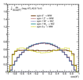
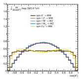
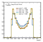
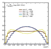
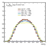
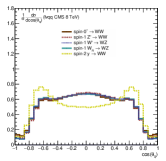
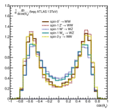
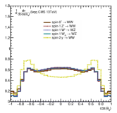
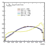
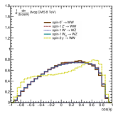
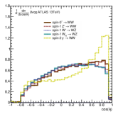
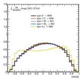
Figure 10: Normalized differential distributions for $\cos\theta^{*}$ (top row), $\cos\theta_{q}$ (middle row), and $\cos\theta_{l}$ (bottom row), for the semi-leptonic final state $\ell\nu qq$, after imposing the ATLAS 8 TeV (first column), CMS 8 TeV (second column), ATLAS 13 TeV (third column), and CMS 13 TeV (last column) analysis cuts. We omit the $\Psi$ angle as it does not have any significant discrimination power.

The asymmetries in the $\cos\theta_{l}$ distributions are the result of contamination by leptonic $\tau$ decays. In particular, the extra neutrinos from the $\tau\to e\nu\nu$ and $\tau\to\mu\nu\nu$ decays skew the reconstruction of the leptonic decay of the $W^{\pm}$, where the additional neutrinos result in a false reconstruction of the rest frame of the $W^{\pm}$. This incorrect rest frame preferentially groups the charged lepton used for the $\cos(\theta_{l})$ calculation closer to the boost vector needed to move to the $W^{\pm}$ rest frame, skewing the $\cos\theta_{l}$ distribution toward the $+1$ edge.

We also note, analogous to the $\ell\ell qq$ final state, the clear cliffs in the $\cos\theta^{*}$ distribution evident in the ATLAS 13 TeV analysis. These cliffs again arise from the $p_{T}^{\ell\nu}>0.4m_{\ell\nu J}$ and $p_{T}^{J}>0.4m_{\ell\nu J}$ cuts, which effectively enforce a $|\cos\theta^{*}|=0.6$ maximum, as discussed before.

V Projections for model discrimination from $4q$ final state

We now quantify the discrimination power between the different spin scenarios using the $CL_{s}$ method Read (2002) to test one signal against another in the $4q$ final state. We define one signal resonance plus dijet background as a signal hypothesis, whereas the test hypothesis is a different spin resonance plus the same dijet background. We use the differential shapes $|\cos\theta^{*}|$, $|\cos\theta_{q}|$, and $|\Psi|$ as individual discriminators as well as a likelihood combination using all three observables.

We perform the pairwise signal hypothesis tests first using shape information alone and second using both shape and rate information. The normalized differential distributions serve as a first test for signal comparisons, because, by construction, different models for a newly discovered resonance will have the same fiducial signal cross section in order to match the observed excess. Hence, even if the 2 TeV excess seen by ATLAS with 8 TeV data is not confirmed by the 13 TeV dataset, our shape-only spin comparisons are indicative of the expected performance of different observables at the initial discovery stage. On the other hand, if data from two different $\sqrt{s}$ working points is available, then the expected scaling from changes in parton distribution functions (PDFs) on various signal rates would be an additional handle to discriminate between models.

Since we adopt the ATLAS 2 TeV diboson excess as our case study, we first normalize the respective differential shapes to this excess. In a 300 GeV window centered at $m_{JJ}=2$ TeV, the ATLAS collaboration observed an excess of 8 events over an expected background of 8.94 events Aad et al. (2015a), where we quote the inclusive diboson tagging requirements. We use this normalization factor, our simulated signal efficiencies, and our simulated PDF rescaling factors to determine the expected number of signal events for each of the other experimental analyses. In the shape only comparisons, the test hypothesis is always normalized to the null hypothesis. The corresponding background expectations, again for inclusive diboson selection cuts, are gleaned from each ATLAS and CMS analysis, albeit with slightly shifted mass windows around the $X$ mass. Since the current ATLAS 13 TeV analysis does not show event counts for an inclusive diboson selection, we estimate the inclusive background expectation from their available data, which we detail in Appendix A.

Not surprisingly, the current discrimination power between different resonance spins is low given the small signal statistics of the 8 TeV and 13 TeV analyses. This situation is expected to dramatically improve, however, with 30 fb^-1 luminosity of 13 TeV data. In Fig. 11, we show the $CL_{s}$ values for a given null hypothesis and various test hypotheses using the current ATLAS 13 TeV and CMS 13 TeV analyses ATL (2015a); CMS (2015) rescaled for 30 fb^-1 of luminosity. We assume a $25\%$ systematic uncertainty on the signal, and $30\%$ on the dijet background. In each row of each figure, the central exclusion limit using only differential distributions is shown as a solid black line, and the corresponding 68% and 95% expected C.L. exclusion limits are shown as the yellow and green bands. The dotted line in each row shows the shift in the central expected exclusion limit if rate information is also added in the signal hypothesis test. These C.L. results are not symmetric under interchange of null hypothesis and test hypotheses, because in the shapes-only $CL_{s}$ analysis, the test hypothesis is always scaled to the null hypothesis, and thus the $S/B$ measure is not equal under the interchange. When rates are included, the Poisson errors are not equal under interchange, and so the resulting C.L. expectations are again not equal.

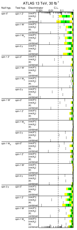
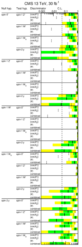
Figure 11: Projected spin sensitivity for the 13 TeV ATLAS (left) and CMS (right) analyses with 30 fb^-1 integrated luminosity. The long vertical dashed line indicates the 95% exclusion C.L. Within each row, the solid black line and the green and yellow shaded areas denote the central expected exclusion and the 68% and 95% likelihood expected exclusion intervals, using only shape information. The dotted black line in each row shows the central expected exclusion limit including rate information, using the 2 TeV excess as the normalization of the respective signal hypotheses.

We see that the most discrimination power comes between the spin-0 and spin-1 cases vs. the spin-2 case, which is expected from the clear distinctions in angular correlations from Fig. 2 for $\cos\theta^{*}$, Fig. 4 for $\cos\theta_{q}$, as well as Fig. 7 for $\Psi$. In particular, the $\cos\theta_{q}$ observable provides significant discrimination, as the spin-2 concavity in the reconstructed differential distribution is opposite that of the spin-0 and spin-1 resonances. We also remark that the $\cos\theta_{q}$ observable has twice the statistical power of the other $\cos\theta^{*}$ and $\Psi$ distributions because each event gives two reconstructed vector boson candidates, and each vector boson candidate contributes one entry to the $\cos\theta_{q}$ distribution.

We also see that CMS generally has stronger projected sensitivity than ATLAS, which is a direct result of the different substructure analyses employed by each experiment. In particular, the ATLAS 13 TeV analysis clusters large radius anti-$k_{T}$ jets with $R=1.0$ and trims these jets using a $k_{T}$ algorithm with $R=0.2$ and hardness measure $z_{\text{min}}=0.05$. We have seen from Fig. 3 that the bulk of the quark pairs from $X\to VV\to 4q$ decays lie within $\Delta R=0.2$, which causes many of the nominal subjets to be merged at the trimming stage.

As a result, the efficiency for the ATLAS 13 TeV analysis to identify two distinct subjets is significantly lower than the corresponding CMS 13 TeV analysis, causing the overall sensitivity to distinguishing spin hypotheses to suffer. The inclusion of rate information shows strong discrimination between the spin-0 null hypothesis compared to the spin-1 hypotheses. This simply follows from the fact that our ad-hoc, gluon-fusion induced, spin-0 diboson resonance enjoys a significant PDF rescaling factor when going from 8 TeV to 13 TeV. In contrast, the $qq^{\prime}$-initiated $Z^{\prime}$, $W^{\prime}$, and $W_{R}$ spin-1 signals are all largely indistinguishable when only considering the $4q$ final state. All of these spin-1 bosons couple to the SM electroweak bosons using the same tree-level Lagrangian structure, which makes it very difficult to disentangle by only considering the $4q$ excess. The small sensitivity afforded by shape and rate information in distinguishing a $Z^{\prime}$ from a $W^{\prime}$ or $W_{R}$ explanation comes from the different PDF scaling from 8 TeV to 13 TeV between $qq^{\prime}$ vs. $q\bar{q}$ initial states. We also note that our signal and background events use inclusive $WW$, $WZ$, and $ZZ$ hadronic diboson tags, and thus additional sensitivity to $W^{\prime}$ or $W_{R}$ discrimination from a $Z^{\prime}$ signal would come from separating these diboson tagging categories.

In some cases, however, the inclusion of rate information decreases the overall discrimination power between signal hypotheses. This is because the shapes-only test magnifies the importance of low event count bins where the signal to background ratio is high, whereas the shapes and rates test loses discrimination power by having an overall lower significance for the given signals. In particular, the linear rescaling we use for matching the signal rates in the rates-only tests overcomes the Poisson statistics governing the low-count bins that is otherwise dominant in the rates and shapes test.

Overall, we see that the spin-2 signal hypothesis will be tested at 95% C.L. using CMS 13 TeV cuts with 30 fb^-1 luminosity. We also project 95% C.L. sensitivity between spin-0 and other spin scenarios by combining rate information with the differential distributions. If a new diboson resonance appears, however, the shape information alone from the current 13 TeV analyses would be insufficient to distinguish spin-0 from spin-1 possibilities.

We conclude this section by discussing the possible improvements to jet substructure analyses that could significantly help the prospects of signal discrimination in a fully hadronic diboson final state. We have seen how the maximum $\Delta\eta_{JJ}$ cut introduces cliffs in $\cos\theta^{*}$ that significantly cut away parts of phase space that would tell a spin-1 signal from other possibilities. Allowing a looser $\Delta\eta_{JJ}$ cut, up to $\Delta\eta_{JJ}\leq 2.2$, for example, would ensure that the extra sinuisoidal oscillation in the spin-2 hypothesis would be more easily distinguished compared to the spin-0 hypothesis and the dijet background, as seen in Fig. 2. Although such a loose cut would lead to an immense increase in multijet background, even intermediate values of $\Delta\eta_{JJ}>1.3$ would already aid discrimination power between the different spin hypotheses. We have also seen that the minimum subjet $p_{T}$ balance requirement removes events above $|\cos\theta_{q}|\approx 0.66$–$0.90$, depending on the $y_{\text{min}}$ cut. These events would have the best discrimination power between spin-2 signals and other possibilities.

The most pernicious effect, however, comes from using a hard angular scale, such as the $k_{T}$ reclustering with $R=0.2$ inherent in the trimming procedure used by ATLAS 13 TeV analysis. This hard angular scale not only causes distinct parton-level decays to merge into single subjets, it also quashes the viability of a post-discovery analysis that builds angular correlations from multiple subjets and introduces significant sculpting effects in $\cos\theta^{*}$ and $\cos\theta_{q}$ distributions. For our 2 TeV case study, the efficiency to find four distinct subjets would increase significantly if a smaller reclustering radius of $R=0.15$ were used, as seen in Figure 3, but the minimum radius for a given resonance mass hypothesis with mass $m_{X}$ can be estimated from $R_{\text{min}}\lesssim 2m_{W/Z}/p_{T,X}\sim m_{W/Z}/m_{X}$.

A jet substructure method optimized for both signal discovery and post-discovery signal discrimination would ameliorate these negative effects. The subjet $p_{T}$ balance requirement and alternate reclustering methods that do not introduce a hard angular scale are thus the most motivated details to modify for a spin-sensitive jet substructure optimization. We reserve a study to address these questions for future work.

VI Conclusion

We have performed a comprehensive study of how angular correlations in resonance decays to four quarks can be preserved, albeit distorted, after effects from hadronization and showering, detector resolution, jet clustering, and $W$ and $Z$ tagging via currently employed jet substructure techniques. We have connected the observed cliffs in $\cos\theta^{*}$ to cuts on the maximum pseudorapidity difference between the parent fat jets, the deficit of events around $\cos\theta^{*},\cos\theta_{q}\approx 0$ to the hard angular scale used in the reclustering of subjets, and the removal of events above $\cos\theta_{q}\approx 0.66$–$0.90$ to the subjet $p_{T}$ balance requirement employed by the various analyses. We have also emphasized the importance of small angular scales for jet substructure reclustering, having seen how large reclustering radii merge distinct decay products of highly boosted vector parents and resulting sensitivity to spin discrimination is greatly reduced.

We recognize that spin discrimination of a new resonance in diboson decays is one facet of a possible post-discovery signal characterization effort. In particular, some of the degeneracies among the various spin-1 signal hypotheses can only be distinguished by observing semi-leptonic diboson decays as well as additional direct decays to fermions. The rates for the latter decays are model dependent features of each given signal hypothesis. In the special case of the 2 TeV excess seen by ATLAS in 8 TeV data, additional discrimination power between possible new physics resonances is afforded by the simple fact that the LHC is now operating at 13 TeV. The different production modes for spin-0, spin-1 neutral, spin-1 charged, and spin-2 resonances obviously scale differently going from $\sqrt{s}=8$ TeV to $\sqrt{s}=13$ TeV, which establishes benchmark expected significances for the different signals as a function of luminosity.

Our work, however, addresses the more general question about the feasibility of using an analysis targetting a resonance in a fully hadronic diboson decay for spin and parity discrimination. It also provides a method for distinguishing longitudinal versus transverse polarizations of electroweak gauge bosons, which is an intrinsic element of analyses aimed at probing unitarity of electroweak boson scattering. A future work will tackle the question of an optimized jet substructure analysis that avoids introducing significant distortions in angular observables and hence enhances the possible spin sensitivity beyond the projections shown in Fig. 11. We also plan to investigate angular correlations in fully hadronic final states with intermediate new physics resonances, as well as the viability of angular observables using Higgs and top substructure methods. Even without any improvement, a spin-2 explanation for the 2 TeV excess will be tested at the 95% C.L. from other spin hypotheses with 30 fb^-1 of 13 TeV luminosity using only shape information, while spin-0 vs. spin-1 discrimination would come from the combination of rate and shape information.

Appendix A ATLAS 13 TeV background extraction, inclusive diboson selection

For our projections on spin sensitivity at 13 TeV LHC, we require the background estimate for inclusive diboson selection cuts. As the current ATLAS 13 TeV analysis ATL (2015a) only provides $WW$, $WZ$, and $ZZ$ event counts, which are not exclusive selection bins because of overlapping $W$ and $Z$ mass windows, we extract the inclusive number of events as follows.

For the mass range $1.0\text{ TeV}<m_{JJ}<2.5$ TeV, the ATLAS analysis specifies that 38 events lie in the overlap region and contribute to all three channels. We thus assign $p\approx\sqrt{38/N}$ as a flat probability for an event with a $W$-tag to also be a $Z$-tagged event and vice versa, where $N$ is the number of events passing inclusive diboson tagging requirements. We can write $N=N_{W^{0}Z^{0}}+N_{W^{0}W^{0}}+N_{Z^{0}Z^{0}}$, where each category is defined exclusively and without overlap. Then,

$$N =N_{WZ}+N_{WW}+N_{ZZ}$$

$$-N_{W^{0}Z^{0}}\cdot\left[\mathcal{P}(Z\text{ in overlap region})+\mathcal{P}(W\text{ in overlap region})+2\mathcal{P}(W\text{ and }Z\text{ in overlap region})\right]$$

$$-N_{W^{0}W^{0}}\cdot\left[\mathcal{P}(\text{one }W\text{ in overlap region})+2\mathcal{P}(\text{both }W\text{ in overlap region})\right]$$

$$-N_{Z^{0}Z^{0}}\cdot\left[\mathcal{P}(\text{one }Z\text{ in overlap region})+2\mathcal{P}(\text{both }Z\text{ in overlap region})\right]\ ,$$ (20)

where factors of 2 in Eq. 20 reflect the fact that this particular event contributes to all three categories and therefore two events need to be subtracted from the total sum. From the ATLAS analysis ATL (2015a), we have $N_{WZ}+N_{WW}+N_{ZZ}=300$, thus

$$N=300 -N_{W^{0}Z^{0}}\left[p(1-p)+p(1-p)+2p^{2}\right]$$

$$-N_{W^{0}W^{0}}\left[2p(1-p)+2p^{2}\right]$$

$$-N_{Z^{0}Z^{0}}\left[2p(1-p)+2p^{2}\right]$$

$$=300 -2Np\ .$$ (21)

Using $p\approx\sqrt{38/N}$, and solving for $N$, we obtain $N\approx 149$, and thus 75 events fall into two diboson categories and 38 events are triply counted, which is very similar to the breakdown of double and triple counted events in the ATLAS 8 TeV analysis Aad et al. (2015a). We use this fraction to estimate the expected number of background events passing the inclusive diboson tagging requirements.

References

- Butterworth et al. (2008) J. M. Butterworth, A. R. Davison, M. Rubin, and G. P. Salam, Phys. Rev. Lett. 100, 242001 (2008), arXiv:0802.2470 [hep-ph] .
- Abdesselam et al. (2011) A. Abdesselam et al., Boost 2010 Oxford, United Kingdom, June 22-25, 2010, Eur. Phys. J. C71, 1661 (2011), arXiv:1012.5412 [hep-ph] .
- Altheimer et al. (2012) A. Altheimer et al., BOOST 2011 Princeton , NJ, USA, 22–26 May 2011, J. Phys. G39, 063001 (2012), arXiv:1201.0008 [hep-ph] .
- Altheimer et al. (2014) A. Altheimer et al., BOOST 2012 Valencia, Spain, July 23-27, 2012, Eur. Phys. J. C74, 2792 (2014), arXiv:1311.2708 [hep-ex] .
- Adams et al. (2015) D. Adams et al., Eur. Phys. J. C75, 409 (2015), arXiv:1504.00679 [hep-ph] .
- Aad et al. (2012) G. Aad et al. (ATLAS), JHEP 05, 128 (2012), arXiv:1203.4606 [hep-ex] .
- Aad et al. (2013) G. Aad et al. (ATLAS), JHEP 09, 076 (2013), arXiv:1306.4945 [hep-ex] .
- Aad et al. (2015a) G. Aad et al. (ATLAS), (2015a), arXiv:1506.00962 [hep-ex] .
- Khachatryan et al. (2014a) V. Khachatryan et al. (CMS), JHEP 08, 173 (2014a), arXiv:1405.1994 [hep-ex] .
- ATL (2015a) Search for resonances with boson-tagged jets in 3.2 fb−1 of p p collisions at = 13 TeV collected with the ATLAS detector, Tech. Rep. ATLAS-CONF-2015-073 (CERN, Geneva, 2015).
- CMS (2015) Search for massive resonances decaying into pairs of boosted W and Z bosons at = 13 TeV, Tech. Rep. CMS-PAS-EXO-15-002 (CERN, Geneva, 2015).
- Aad et al. (2014) G. Aad et al. (ATLAS), Phys. Lett. B737, 223 (2014), arXiv:1406.4456 [hep-ex] .
- Aad et al. (2015b) G. Aad et al. (ATLAS), Eur. Phys. J. C75, 69 (2015b), arXiv:1409.6190 [hep-ex] .
- Aad et al. (2015c) G. Aad et al. (ATLAS), Eur. Phys. J. C75, 209 (2015c), [Erratum: Eur. Phys. J.C75,370(2015)], arXiv:1503.04677 [hep-ex] .
- Aad et al. (2015d) G. Aad et al. (ATLAS), (2015d), arXiv:1512.05099 [hep-ex] .
- Khachatryan et al. (2015a) V. Khachatryan et al. (CMS), Phys. Lett. B740, 83 (2015a), arXiv:1407.3476 [hep-ex] .
- Khachatryan et al. (2014b) V. Khachatryan et al. (CMS), JHEP 08, 174 (2014b), arXiv:1405.3447 [hep-ex] .
- Brehmer et al. (2015a) J. Brehmer et al., (2015a), arXiv:1512.04357 [hep-ph] .
- ATL (2015b) Search for resonance production in the final state at TeV with the ATLAS detector at the LHC, Tech. Rep. ATLAS-CONF-2015-075 (CERN, Geneva, 2015).
- ATL (2015c) Search for diboson resonances in the llqq final state in pp collisions at = 13 TeV with the ATLAS detector, Tech. Rep. ATLAS-CONF-2015-071 (CERN, Geneva, 2015).
- ATL (2015d) Search for diboson resonances in the final state in collisions at 13 TeV with the ATLAS detector, Tech. Rep. ATLAS-CONF-2015-068 (CERN, Geneva, 2015).
- Dobrescu and Liu (2015a) B. A. Dobrescu and Z. Liu, Phys. Rev. Lett. 115, 211802 (2015a), arXiv:1506.06736 [hep-ph] .
- Dobrescu and Liu (2015b) B. A. Dobrescu and Z. Liu, JHEP 10, 118 (2015b), arXiv:1507.01923 [hep-ph] .
- Brehmer et al. (2015b) J. Brehmer, J. Hewett, J. Kopp, T. Rizzo, and J. Tattersall, JHEP 10, 182 (2015b), arXiv:1507.00013 [hep-ph] .
- Dobrescu and Fox (2015) B. A. Dobrescu and P. J. Fox, (2015), arXiv:1511.02148 [hep-ph] .
- Anchordoqui et al. (2015) L. A. Anchordoqui, I. Antoniadis, H. Goldberg, X. Huang, D. Lust, and T. R. Taylor, Phys. Lett. B749, 484 (2015), arXiv:1507.05299 [hep-ph] .
- Aad et al. (2015e) G. Aad et al. (ATLAS), Phys. Rev. D91, 052007 (2015e), arXiv:1407.1376 [hep-ex] .
- Khachatryan et al. (2015b) V. Khachatryan et al. (CMS), Phys. Rev. D91, 052009 (2015b), arXiv:1501.04198 [hep-ex] .
- Aad et al. (2016a) G. Aad et al. (ATLAS), Phys. Lett. B754, 302 (2016a), [Phys. Lett.B754,302(2016)], arXiv:1512.01530 [hep-ex] .
- Khachatryan et al. (2015c) V. Khachatryan et al. (CMS), (2015c), arXiv:1512.01224 [hep-ex] .
- Aad et al. (2015f) G. Aad et al. (ATLAS), Eur. Phys. J. C75, 263 (2015f), arXiv:1503.08089 [hep-ex] .
- Khachatryan et al. (2015d) V. Khachatryan et al. (CMS), Phys. Lett. B748, 255 (2015d), arXiv:1502.04994 [hep-ex] .
- Khachatryan et al. (2015e) V. Khachatryan et al. (CMS), (2015e), arXiv:1506.01443 [hep-ex] .
- Khachatryan et al. (2016) V. Khachatryan et al. (CMS), (2016), arXiv:1601.06431 [hep-ex] .
- ATL (2015e) Search for new resonances decaying to a W or Z boson and a Higgs boson in the , , and channels in collisions at TeV with the ATLAS detector, Tech. Rep. ATLAS-CONF-2015-074 (CERN, Geneva, 2015).
- Chen and Nomura (2015a) C.-H. Chen and T. Nomura, (2015a), arXiv:1509.02039 [hep-ph] .
- Chen and Nomura (2015b) C.-H. Chen and T. Nomura, Phys. Lett. B749, 464 (2015b), arXiv:1507.04431 [hep-ph] .
- Omura et al. (2015) Y. Omura, K. Tobe, and K. Tsumura, Phys. Rev. D92, 055015 (2015), arXiv:1507.05028 [hep-ph] .
- Chao (2015) W. Chao, (2015), arXiv:1507.05310 [hep-ph] .
- Aristizabal Sierra et al. (2015) D. Aristizabal Sierra, J. Herrero-Garcia, D. Restrepo, and A. Vicente, (2015), arXiv:1510.03437 [hep-ph] .
- Petersson and Torre (2015) C. Petersson and R. Torre, (2015), arXiv:1508.05632 [hep-ph] .
- Allanach et al. (2015a) B. C. Allanach, P. S. B. Dev, and K. Sakurai, (2015a), arXiv:1511.01483 [hep-ph] .
- Chiang et al. (2015) C.-W. Chiang, H. Fukuda, K. Harigaya, M. Ibe, and T. T. Yanagida, JHEP 11, 015 (2015), arXiv:1507.02483 [hep-ph] .
- Cacciapaglia et al. (2015) G. Cacciapaglia, A. Deandrea, and M. Hashimoto, Phys. Rev. Lett. 115, 171802 (2015), arXiv:1507.03098 [hep-ph] .
- Fukano et al. (2015a) H. S. Fukano, M. Kurachi, S. Matsuzaki, K. Terashi, and K. Yamawaki, Phys. Lett. B750, 259 (2015a), arXiv:1506.03751 [hep-ph] .
- Franzosi et al. (2015) D. B. Franzosi, M. T. Frandsen, and F. Sannino, (2015), arXiv:1506.04392 [hep-ph] .
- Thamm et al. (2015) A. Thamm, R. Torre, and A. Wulzer, Phys. Rev. Lett. 115, 221802 (2015), arXiv:1506.08688 [hep-ph] .
- Bian et al. (2015a) L. Bian, D. Liu, and J. Shu, (2015a), arXiv:1507.06018 [hep-ph] .
- Fritzsch (2015) H. Fritzsch, (2015), arXiv:1507.06499 [hep-ph] .
- Lane and Prichett (2015) K. Lane and L. Prichett, (2015), arXiv:1507.07102 [hep-ph] .
- Low et al. (2015) M. Low, A. Tesi, and L.-T. Wang, Phys. Rev. D92, 085019 (2015), arXiv:1507.07557 [hep-ph] .
- Fukano et al. (2015b) H. S. Fukano, S. Matsuzaki, K. Terashi, and K. Yamawaki, (2015b), arXiv:1510.08184 [hep-ph] .
- Cacciapaglia and Frandsen (2015) G. Cacciapaglia and M. T. Frandsen, Phys. Rev. D92, 055035 (2015), arXiv:1507.00900 [hep-ph] .
- Allanach et al. (2015b) B. C. Allanach, B. Gripaios, and D. Sutherland, Phys. Rev. D92, 055003 (2015b), arXiv:1507.01638 [hep-ph] .
- Bian et al. (2015b) L. Bian, D. Liu, J. Shu, and Y. Zhang, (2015b), arXiv:1509.02787 [hep-ph] .
- Bhattacherjee et al. (2015) B. Bhattacherjee, P. Byakti, C. K. Khosa, J. Lahiri, and G. Mendiratta, (2015), arXiv:1511.02797 [hep-ph] .
- Xue (2015) S.-S. Xue, (2015), arXiv:1506.05994 [hep-ph] .
- Gao et al. (2015) Y. Gao, T. Ghosh, K. Sinha, and J.-H. Yu, Phys. Rev. D92, 055030 (2015), arXiv:1506.07511 [hep-ph] .
- Heeck and Patra (2015) J. Heeck and S. Patra, Phys. Rev. Lett. 115, 121804 (2015), arXiv:1507.01584 [hep-ph] .
- Bhupal Dev and Mohapatra (2015) P. S. Bhupal Dev and R. N. Mohapatra, Phys. Rev. Lett. 115, 181803 (2015), arXiv:1508.02277 [hep-ph] .
- Deppisch et al. (2015) F. F. Deppisch, L. Graf, S. Kulkarni, S. Patra, W. Rodejohann, N. Sahu, and U. Sarkar, (2015), arXiv:1508.05940 [hep-ph] .
- Aydemir et al. (2015) U. Aydemir, D. Minic, C. Sun, and T. Takeuchi, (2015), arXiv:1509.01606 [hep-ph] .
- Awasthi et al. (2015) R. L. Awasthi, P. S. B. Dev, and M. Mitra, (2015), arXiv:1509.05387 [hep-ph] .
- Ko and Nomura (2015) P. Ko and T. Nomura, (2015), arXiv:1510.07872 [hep-ph] .
- Collins and Ng (2015) J. H. Collins and W. H. Ng, (2015), arXiv:1510.08083 [hep-ph] .
- Aguilar-Saavedra and Joaquim (2015) J. A. Aguilar-Saavedra and F. R. Joaquim, (2015), arXiv:1512.00396 [hep-ph] .
- Aydemir (2016) U. Aydemir, Int. J. Mod. Phys. A31, 1650034 (2016), arXiv:1512.00568 [hep-ph] .
- Evans et al. (2015) J. L. Evans, N. Nagata, K. A. Olive, and J. Zheng, (2015), arXiv:1512.02184 [hep-ph] .
- Das et al. (2016) A. Das, N. Nagata, and N. Okada, JHEP 03, 049 (2016), arXiv:1601.05079 [hep-ph] .
- Hisano et al. (2015) J. Hisano, N. Nagata, and Y. Omura, Phys. Rev. D92, 055001 (2015), arXiv:1506.03931 [hep-ph] .
- Alves et al. (2015) A. Alves, A. Berlin, S. Profumo, and F. S. Queiroz, JHEP 10, 076 (2015), arXiv:1506.06767 [hep-ph] .
- Faraggi and Guzzi (2015) A. E. Faraggi and M. Guzzi, Eur. Phys. J. C75, 537 (2015), arXiv:1507.07406 [hep-ph] .
- Li et al. (2015) T. Li, J. A. Maxin, V. E. Mayes, and D. V. Nanopoulos, (2015), arXiv:1509.06821 [hep-ph] .
- Wang et al. (2015) Z.-W. Wang, F. S. Sage, T. G. Steele, and R. B. Mann, (2015), arXiv:1511.02531 [hep-ph] .
- Allanach et al. (2015c) B. Allanach, F. S. Queiroz, A. Strumia, and S. Sun, (2015c), arXiv:1511.07447 [hep-ph] .
- Feng et al. (2015) W.-Z. Feng, Z. Liu, and P. Nath, (2015), arXiv:1511.08921 [hep-ph] .
- Cheung et al. (2015) K. Cheung, W.-Y. Keung, P.-Y. Tseng, and T.-C. Yuan, Phys. Lett. B751, 188 (2015), arXiv:1506.06064 [hep-ph] .
- Cao et al. (2015) Q.-H. Cao, B. Yan, and D.-M. Zhang, Phys. Rev. D92, 095025 (2015), arXiv:1507.00268 [hep-ph] .
- Abe et al. (2015a) T. Abe, R. Nagai, S. Okawa, and M. Tanabashi, Phys. Rev. D92, 055016 (2015a), arXiv:1507.01185 [hep-ph] .
- Abe et al. (2015b) T. Abe, T. Kitahara, and M. M. Nojiri, (2015b), arXiv:1507.01681 [hep-ph] .
- Fukano et al. (2015c) H. S. Fukano, S. Matsuzaki, and K. Yamawaki, (2015c), arXiv:1507.03428 [hep-ph] .
- Appelquist et al. (2015) T. Appelquist, Y. Bai, J. Ingoldby, and M. Piai, (2015), arXiv:1511.05473 [hep-ph] .
- Das et al. (2015) K. Das, T. Li, S. Nandi, and S. K. Rai, (2015), arXiv:1512.00190 [hep-ph] .
- Sanz (2015) V. Sanz, (2015), arXiv:1507.03553 [hep-ph] .
- Terazawa and Yasue (2015) H. Terazawa and M. Yasue, (2015), arXiv:1508.00172 [hep-ph] .
- Aguilar-Saavedra (2015) J. A. Aguilar-Saavedra, JHEP 10, 099 (2015), arXiv:1506.06739 [hep-ph] .
- Kim et al. (2015) D. Kim, K. Kong, H. M. Lee, and S. C. Park, (2015), arXiv:1507.06312 [hep-ph] .
- Liew and Shirai (2015) S. P. Liew and S. Shirai, JHEP 11, 191 (2015), arXiv:1507.08273 [hep-ph] .
- Arnan et al. (2015) P. Arnan, D. Espriu, and F. Mescia, (2015), arXiv:1508.00174 [hep-ph] .
- Fichet and von Gersdorff (2015) S. Fichet and G. von Gersdorff, (2015), arXiv:1508.04814 [hep-ph] .
- Sajjad (2015) A. Sajjad, (2015), arXiv:1511.02244 [hep-ph] .
- Aad et al. (2015g) G. Aad et al. (ATLAS), Eur. Phys. J. C75, 476 (2015g), arXiv:1506.05669 [hep-ex] .
- Aad et al. (2016b) G. Aad et al. (ATLAS), Eur. Phys. J. C76, 6 (2016b), arXiv:1507.04548 [hep-ex] .
- Khachatryan et al. (2015f) V. Khachatryan et al. (CMS), Phys. Rev. D92, 012004 (2015f), arXiv:1411.3441 [hep-ex] .
- Khachatryan et al. (2015g) V. Khachatryan et al. (CMS), Eur. Phys. J. C75, 212 (2015g), arXiv:1412.8662 [hep-ex] .
- Cabibbo and Maksymowicz (1965) N. Cabibbo and A. Maksymowicz, Phys. Rev. 137, B438 (1965), [Erratum: Phys. Rev.168,1926(1968)].
- Dell’Aquila and Nelson (1986a) J. R. Dell’Aquila and C. A. Nelson, Phys. Rev. D33, 80 (1986a).
- Dell’Aquila and Nelson (1986b) J. R. Dell’Aquila and C. A. Nelson, Phys. Rev. D33, 93 (1986b).
- Nelson (1988) C. A. Nelson, Proceedings, 23RD International Conference on High Energy Physics, JULY 16-23, 1986, Berkeley, CA, Phys. Rev. D37, 1220 (1988).
- Gao et al. (2010) Y. Gao, A. V. Gritsan, Z. Guo, K. Melnikov, M. Schulze, and N. V. Tran, Phys. Rev. D81, 075022 (2010), arXiv:1001.3396 [hep-ph] .
- Bolognesi et al. (2012) S. Bolognesi, Y. Gao, A. V. Gritsan, K. Melnikov, M. Schulze, N. V. Tran, and A. Whitbeck, Phys. Rev. D86, 095031 (2012), arXiv:1208.4018 [hep-ph] .
- Chen et al. (2013) Y. Chen, N. Tran, and R. Vega-Morales, JHEP 01, 182 (2013), arXiv:1211.1959 [hep-ph] .
- Chen et al. (2015) Y. Chen, E. Di Marco, J. Lykken, M. Spiropulu, R. Vega-Morales, and S. Xie, JHEP 01, 125 (2015), arXiv:1401.2077 [hep-ex] .
- Chen et al. (2014) Y. Chen, E. Di Marco, J. Lykken, M. Spiropulu, R. Vega-Morales, and S. Xie, (2014), arXiv:1410.4817 [hep-ph] .
- Dokshitzer et al. (1997) Y. L. Dokshitzer, G. D. Leder, S. Moretti, and B. R. Webber, JHEP 08, 001 (1997), arXiv:hep-ph/9707323 [hep-ph] .
- Ellis et al. (2009) S. D. Ellis, C. K. Vermilion, and J. R. Walsh, Phys. Rev. D80, 051501 (2009), arXiv:0903.5081 [hep-ph] .
- Ellis et al. (2010) S. D. Ellis, C. K. Vermilion, and J. R. Walsh, Phys. Rev. D81, 094023 (2010), arXiv:0912.0033 [hep-ph] .
- Thaler and Van Tilburg (2011) J. Thaler and K. Van Tilburg, JHEP 03, 015 (2011), arXiv:1011.2268 [hep-ph] .
- Thaler and Van Tilburg (2012) J. Thaler and K. Van Tilburg, JHEP 02, 093 (2012), arXiv:1108.2701 [hep-ph] .
- Krohn et al. (2010) D. Krohn, J. Thaler, and L.-T. Wang, JHEP 02, 084 (2010), arXiv:0912.1342 [hep-ph] .
- Catani et al. (1993) S. Catani, Y. L. Dokshitzer, M. H. Seymour, and B. R. Webber, Nucl. Phys. B406, 187 (1993).
- Larkoski et al. (2013) A. J. Larkoski, G. P. Salam, and J. Thaler, JHEP 06, 108 (2013), arXiv:1305.0007 [hep-ph] .
- Larkoski et al. (2014) A. J. Larkoski, I. Moult, and D. Neill, JHEP 12, 009 (2014), arXiv:1409.6298 [hep-ph] .
- Larkoski et al. (2015) A. J. Larkoski, I. Moult, and D. Neill, (2015), arXiv:1507.03018 [hep-ph] .
- Alloul et al. (2014) A. Alloul, N. D. Christensen, C. Degrande, C. Duhr, and B. Fuks, Comput. Phys. Commun. 185, 2250 (2014), arXiv:1310.1921 [hep-ph] .
- Alwall et al. (2011) J. Alwall, M. Herquet, F. Maltoni, O. Mattelaer, and T. Stelzer, JHEP 06, 128 (2011), arXiv:1106.0522 [hep-ph] .
- Pappadopulo et al. (2014) D. Pappadopulo, A. Thamm, R. Torre, and A. Wulzer, JHEP 09, 060 (2014), arXiv:1402.4431 [hep-ph] .
- Randall and Sundrum (1999a) L. Randall and R. Sundrum, Phys. Rev. Lett. 83, 3370 (1999a), arXiv:hep-ph/9905221 [hep-ph] .
- Randall and Sundrum (1999b) L. Randall and R. Sundrum, Phys. Rev. Lett. 83, 4690 (1999b), arXiv:hep-th/9906064 [hep-th] .
- Hagiwara et al. (2008) K. Hagiwara, J. Kanzaki, Q. Li, and K. Mawatari, Eur. Phys. J. C56, 435 (2008), arXiv:0805.2554 [hep-ph] .
- Sjöstrand et al. (2015) T. Sjöstrand, S. Ask, J. R. Christiansen, R. Corke, N. Desai, P. Ilten, S. Mrenna, S. Prestel, C. O. Rasmussen, and P. Z. Skands, Comput. Phys. Commun. 191, 159 (2015), arXiv:1410.3012 [hep-ph] .
- de Favereau et al. (2014) J. de Favereau, C. Delaere, P. Demin, A. Giammanco, V. Lemaître, A. Mertens, and M. Selvaggi (DELPHES 3), JHEP 02, 057 (2014), arXiv:1307.6346 [hep-ex] .
- Cacciari et al. (2012) M. Cacciari, G. P. Salam, and G. Soyez, Eur. Phys. J. C72, 1896 (2012), arXiv:1111.6097 [hep-ph] .
- Cacciari et al. (2008) M. Cacciari, G. P. Salam, and G. Soyez, JHEP 04, 063 (2008), arXiv:0802.1189 [hep-ph] .
- Khachatryan et al. (2014c) V. Khachatryan et al. (CMS), JHEP 12, 017 (2014c), arXiv:1410.4227 [hep-ex] .
- Hackstein and Spannowsky (2010) C. Hackstein and M. Spannowsky, Phys. Rev. D82, 113012 (2010), arXiv:1008.2202 [hep-ph] .
- Englert et al. (2010) C. Englert, C. Hackstein, and M. Spannowsky, Phys. Rev. D82, 114024 (2010), arXiv:1010.0676 [hep-ph] .
- Read (2002) A. L. Read, Advanced Statistical Techniques in Particle Physics. Proceedings, Conference, Durham, UK, March 18-22, 2002, J. Phys. G28, 2693 (2002), [,11(2002)].