Amoeboid swimming in a channel

Abstract

Several micro-organisms, such as bacteria, algae, or spermatozoa, use flagellar or ciliary activity to swim in a fluid, while many other micro-organisms instead use ample shape deformation, described as amoeboid, to propel themselves by either crawling on a substrate or swimming. Many eukaryotic cells were believed to require an underlying substratum to migrate (crawl) by using membrane deformation (like blebbing or generation of lamellipodia) but there is now increasing evidence that a large variety of cells (including those of the immune system) can migrate without the assistance of focal adhesion, allowing them to swim as efficiently as they can crawl. This paper details the analysis of amoeboid swimming in a confined fluid by modeling the swimmer as an inextensible membrane deploying local active forces (with zero total force and torque). The swimmer displays a rich behavior: it may settle into a straight trajectory in the channel or navigate from one wall to the other depending on its confinement. The nature of the swimmer is also found to be affected by confinement: the swimmer can behave, on the average over one swimming cycle, as a pusher at low confinement, and becomes a puller at higher confinement, or vice versa. The swimmer’s nature is thus not an intrinsic property. The scaling of the swimmer velocity $V$ with the force amplitude $A$ is analyzed in detail showing that at small enough $A$, $V\sim A^{2}/\eta^{2}$ (where $\eta$ is the viscosity of the ambient fluid), whereas at large enough $A$, $V$ is independent of the force and is determined solely by the stroke cycle frequency and swimmer size. This finding starkly contrasts with currently known results found from swimming models where motion is based on ciliary and flagellar activity, where $V\sim A/\eta$. To conclude, two definitions of efficiency as put forward in the literature are analyzed with distinct outcomes. We find that one type of efficiency has an optimum as a function of confinement while the other does not. Future perspectives are outlined.

I Introduction

In the past decade, the problem of swimming in a low Reynolds number environment has attracted much attention from biology, physics, applied mathematics, computer science, chemistry, and mechanical engineering. Many kinds of motile unicellular micro-organisms living in the world of low Reynolds number Lauga and Powers (2009); Saintillan and Shelley (2012) use a variety of strategies to propel themselves in liquids. So far most of the studies have been directed towards organisms employing flagellum and cilium activity. Some typical examples are spermatozoa Fauci and McDonald (1995); Kantsler et al. (2013), bacteria such as E. coli Lauga et al. (2006); Berke et al. (2008) and Bacillus subtilis Sokolov and Aranson (2009) (examples of the so-called pusher), algae like Chlamydomonas Reinhardtii (an example of puller) Drescher et al. (2009); Guasto et al. (2010); Garcia et al. (2011); Kantsler et al. (2013), Volvox Drescher et al. (2009, 2010) and Paramecium Jana et al. (2012); Zhang et al. (2015) (examples of neutral swimmers). There has also been great interest in designing artificial microswimmers driven by different external fields, such as a rotating magnetic field Zhang et al. (2009), a catalytic reaction field Paxton et al. (2004), and so on.

Another category of swimmers, much less studied until now, employ amoeboid swimming (AS). Amoeboid movement is the most common mode of locomotion in eukaryotic cells (monocytes, neutrophils, macrophages, cancerous cells, etc.). The denomination amoeboid motion generically refers to motility due to shape deformation, and can be performed in a solution (like swimming) or on a substratum (crawling). Eutreptiella Gymnastica Throndsen (1969), a common representative of euglenids of marine phytoplankton, is a prototypical example of an amoeboid swimmer. On the other hand, many eukaryotic cells, such as leucocytes, fibroblasts, etc., which use ample membrane deformation for motility have been categorized as crawlers, that is, as micro-organisms which use focal adhesion on a substratum to move forward. Crawling has been extensively studied in the biological and biophysical literatures D’Ambrosio and Sinigaglia (2004); Entschladen and Zänker (2009) for it plays an essential role in many physiological and pathological processes including embryonic development, wound healing, immune response and cancer metastasis. It must be emphasized that there is yet no general consensus about the ’amoeboid’ denomination for crawling cells. Some authors make a distinction between amoeboid cells and mesenchymal cells, where in the latter category the adhesion is so strong that the shape change may be minor and not appearing as a predominant factor for motion (see references Lämmermann and Sixt (2009); Liu et al. (2015)). It has been seen that sometimes a cell may switch from mesenchymal to amoeboid motion under confinement Liu et al. (2015). In the present study amoeboid motion refers to any motion that requires a shape change to move forward.

Several recent studies have been directed toward elucidating the role of focal adhesion in the migration process. One such study revealed that adhesion-based crawling is not necessarily a pre-requisite for cell locomotion once leukocytes transmigrate across the endothelium Lämmermann et al. (2008). Adhesion molecules would then serve only to stop moving leucocytes in the blood stream, making them adhere to the endothelium before transmigration. Studies in vitro have shown that integrins (the principal cell adhesion molecules) do not contribute to migration in three-dimensional environments (in suspension with fibrous material, mimicking extracellular matrix of tissues)Lämmermann et al. (2008). Instead these cells migrate using actin polymerization, which leads to membrane protrusion on the leading front. It is debatedLiu et al. (2015); Hawkins et al. (2009) as to whether or not cell contact with fibrous material, without any specific adhesion, is necessary in order to assist locomotion. A more recent study supports the idea of pure swimming in cells of the immune system (neutrophils), and in dictyostelium Barry and Bretscher (2010); it has been found that these cells, when far from the substrate, move toward a chemo-attractant. A remarkable result shows that they can swim Barry and Bretscher (2010) with speeds of comparable magnitude to those on a solid substrate (crawling). Other recent experimental studies focused Bergert et al. (2015) on cell motion in a confined geometry showed that a blebbing cell can undergo movement through nonspecific adhesion, but only thanks to a solid-like friction from the substrate. In other words, this corresponds to a situation where the cell is in ”physical” contact with the substrate on which the cell might lean, in a fashion similar to the case of a cell leaning on a fibrous (or extracellular) material, but with no specific adhesion needed.

The above studies strongly support the idea that adhesion is not necessary for migration. In some reported cases Barry and Bretscher (2010) cells may even bypass contact with the substrate and perform pure swimming in a fluid. There seems thus to be a whole spectrum of possibilities relevant for cell migration, ranging from specific-adhesion assisted crawling, through pure non-specific friction with an elastic substratum, up to pure swimming in a solution. Thus an important task in research concerns bridging the gaps between pure swimming and motion by physical contact (solid-like friction), up to crawling.

Our goal is to first isolate different effects and then progressively increase the degree of complexity to reveal the imbricated nature of cell motility. To this end, we have systematically analyzed amoeboid motion in the pure swimming case and studied the effect of bounding walls. Though there is no direct friction (no contact) with walls, the fluid between the swimmer and the walls serves as a support for transmitting frictional forces between the swimmer and the walls. It must be noted, however, that while confinement (if not too strong in our case) promotes migration, the presence of bounding walls is not required; motility can take place in a completely unbounded medium, provided that the shape change is not reversible in time, as required by the Purcell’s scallop theorem Purcell (1977).

Several models of directed self-propulsion by large shape deformation have been explored in the literature Avron et al. (2004); Ohta and Ohkuma (2009); Hiraiwa et al. (2011); Alouges et al. (2011); Arroyo et al. (2012); Vilfan (2012); Loheac et al. (2013); Farutin et al. (2013); Wu et al. (2015). In two recent studies we introduced a model in which Farutin et al. (2013); Wu et al. (2015) the swimmer is considered as made of an inextensible membrane enclosing a constant volume of liquid and exerting a set of normal forces leading to deformations of the swimmer and to propulsion. The first study Farutin et al. (2013) dealt with purely unconfined three dimensional (3D) geometry; the more recent work was dedicated to a confined swimmer in two dimensions (2D) Wu et al. (2015), a situation revealing several puzzling phenomena which we will look at later. Here we report on several new issues emerging for a confined amoeboid swimmer. For example, we show that the velocity of migration has a nontrivial scaling with the force and address the notion of efficiency by testing two definitions. We shall see, for example, that for certain confinement, the efficiency attains an optimal value. We will discuss the space-scanning capability of the swimmer, where we find that generally the swimmer can scan about $90\%$ of the available space.

This paper is organized as follows: in Section II, we present a minimal model for AS. In Section III the two numerical methods used in this study are briefly detailed: the boundary integral method (BIM) Thiébaud and Misbah (2013); Wu et al. (2015) and the immersed boundary method (IBM) Hu et al. (2014). In Section IV, we present the main results regarding an axially moving swimmer. In Section V we discuss both the peculiar behavior of the velocity as a function of confinement and the power consumption problem. Section VI analyzes the swimmer efficiency. Section VII is devoted to different dynamical motions. Conclusions and perspectives constitute the subject of Section VIII. Some technical details are given in an Appendix.

II Model and simulation method

II.1 Amoeboid swimmer model

For simplicity, and due to the high computational cost, we consider a 2D geometry. An amoeboid swimmer (AS) is modeled as a membrane immersed in a Newtonian fluid domain of a given viscosity $\eta$. The encapsulated fluid is taken to have the same viscosity, for simplicity. We consider the pure Stokes regime (no inertia). An effective radius of the swimmer is defined as $R_{0}=\sqrt{A_{0}/\pi}$, where $A_{0}$ is the enclosed area. We define an excess perimeter (excess counted from a circular shape) $\Gamma=L_{0}/(2\pi R_{0})-1$ to describe the degree of deflation of swimmer shape. $\Gamma=0$ represents a circular shape, whereas a large $\Gamma$ refers to a swimmer with ample shape deformations. The perimeter $L_{0}$ of the swimmer membrane is taken to be constant due to the inextensibility of the membrane. Extensible membranes can be dealt with as well, but our goal is to consider a minimal model from which to capture basic features before refinement. The swimmer is confined between two rigid walls separated by a distance $W$. We impose the no-slip boundary condition at the walls. A schematic representation of the studied system with some useful notations is shown in Fig. 1.

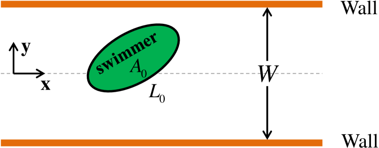
Figure 1: (Color online) A schematic representation of the system and some useful notations. The swimmer has internal area $A_{0}$ and perimeter $L_{0}$.

We consider certain forces deployed by the swimmer’s internal machinery , with a certain distribution at the membrane. These are called the active forces and denoted as ${\mathbf{F}}_{a}$, and depend on the position of a material point of the membrane and on time (see below). The active forces have a natural tendency to expand (or compress) the membrane which will resist thanks to its intrinsic cohesive forces, resulting in a tension-like reaction. Since we are considering a purely incompressible membrane, the tension is such that the local arclength should remain constant in the course of time.

II.2 The choice of the active forces

The total force density (force per unit area) at the membrane is thus composed of an active part and a passive part, and can be written as

$${\mathbf{F}}=F_{a}{\mathbf{n}}-\zeta c{\mathbf{n}}+\frac{\partial\zeta}{\partial s}{\mathbf{t}},$$ (1)

where ${F_{a}}{\mathbf{n}}$ is the active force specified below and which we take to be directed along the normal direction, with ${\mathbf{n}}$ denoting the unit normal vector. $\zeta(s,t)$ is a Lagrange multiplier that enforces local membrane inextensibility, $c$ is the curvature, ${\mathbf{t}}$ is the unit tangent vector, and $s$ is the arclength. Stresses (due to flow and active forces) vary, in general, from one membrane point to another, so the membrane deploys a local opposing tension that tends to keep the local membrane length $ds$ constant in the course of time. In a vectorial form the tension is given by $\zeta(s)\mathbf{t}(s)$. Consider two neighboring membrane points at positions $s$ and $s+ds$, respectively. The resultant tension felt by the membrane element $ds$ is given by $\zeta(s+ds)\mathbf{t}(s+ds)-\zeta(s){\mathbf{t}}(s)=[(\partial\zeta/\partial s){\mathbf{t}}+\zeta\partial{\mathbf{t}}/\partial s]ds+O(ds^{2})$. The force per unit length is obtained by dividing the above result by $ds$. Using the geometrical result $\partial{\mathbf{t}}/\partial s=-c{\mathbf{n}}$ and taking the limit $ds\rightarrow 0$, we obtain the tension force in eqn (1).

Since the boundary of the swimmer is a closed curve, it is convenient to decompose the active force into Fourier series

$${F}_{a}(\alpha,t)=\sum_{k=-k_{max},|k|\neq 0,1}^{k=k_{max}}\hat{F}_{k}(t)e^{ik\alpha},$$ (2)

where we have defined the normalized arc length $\alpha=2\pi s/L_{0}$. We must impose that the total force and the total torque equal zero:

$$\oint{\mathbf{F}}ds=0,\;\;\;\oint{\mathbf{r}}\times{\mathbf{F}}ds=0.$$ (3)

The integrals are performed over the swimmer perimeter. This leads to three equations which are linear in terms of the active forces . The coefficients of the system depend on the actual shape, which is unknown a priori. Conditions given by Eqn (3) impose linear relations between the amplitudes $\hat{F}_{k}(t)$. However, these relations did not allow us to easily reduce the number of independent force amplitudes because the resulting system was occasionally ill-conditioned. We solved this problem by adding an extra term to the active force, ${\mathbf{F}_{0}}+\tilde{F}_{0}\mathbf{t}.$ The first contribution is constant, and the second is purely tangential. We then use eqn (3) to express $\tilde{F}_{0}$ and ${\mathbf{F}_{0}}$ in terms of $\hat{F}_{k}^{\prime}s$. The virtue of this approach is the following: using the force and torque balance equations we easily see that in the linear system the coefficient in front of ${\mathbf{F}_{0}}$ is proportional to the swimmer perimeter, whereas the coefficient in front of $\tilde{F}_{0}$ is proportional to the swimmer area, so that the matrix of the system of equations which multiplies the vector $({\mathbf{F}_{0}},\tilde{F}_{0}\mathbf{t})$, is non-singular whatever the swimmer evolution, since the perimeter and area are definite positive quantities.

Our strategy is to keep the model as simple as possible, and therefore we will limit the expansion (2) to $k_{max}=3$. The mode with $k=0$ does not play a role because the fluid is incompressible ($k=0$ corresponds to a homogeneous pressure jump across the membrane). For simplicity we set $F_{1}=0$. We are thus left with two complex amplitudes $\hat{F}_{2}$ and $\hat{F}_{3}$ . Once more for simplicity, the imaginary parts of $\hat{F}_{2}$ and $\hat{F}_{3}$ are set to zero, so the active force used in this work is taken to be

$$F_{a}(\alpha,t)=2F_{2}(t)\cos(2\alpha)+2F_{3}(t)\cos(3\alpha).$$ (4)

$F_{2}$ and $F_{3}$ are time-dependent quantities expressing the cell’s execution of a cyclic motion in order to move forwards. According to Purcell’s theorem Purcell (1977), this cyclic motion should not be reversible in time owing to the invariance of the Stokes equations upon time reversal. Based on our first study on amoeboid motion Farutin et al. (2013) we shall make a simple choice for time dependence

$$F_{2}(t)=-A_{2}\cos(\omega t),\;\;\;F_{3}(t)=A_{3}\sin(\omega t).$$ (5)

where for simplicity $A_{2}$ and $A_{3}$ are taken to be equal ($A_{2}=A_{3}=A$). We are thus left with four parameters characterizing the force distribution, $A$, the scalar $\tilde{F}_{0}$ and the two components of ${\mathbf{F}_{0}}$. Use of condition (3) allows one to express the three force components $F_{0x}$, $F_{0y}$ and $\tilde{F}_{0}$ as functions of $A$ for a given shape of the swimmer. We are thus left with a single parameter monitoring the force, namely, the amplitude $A$.

Note that the total force and the total torque of our passive force related to $\zeta$ (eqn (1)) vanish automatically. Indeed, the passive force can be written as a functional derivative of an energy (see Ref. Kaoui et al. (2008))

$${\mathbf{F}}^{\rm mem}=-\frac{\delta E({\mathbf{r}}(s))}{\delta{\mathbf{r}}},$$ (6)

where $\delta/\delta{\mathbf{r}}$ is the functional derivative. Since this energy is intrinsic to the membrane, any rigid translation or rotation leaves it invariant. Let $\delta{\mathbf{r}}$ be the displacement of a given point on the membrane during a time interval $\delta t$, corresponding to a rigid translation or rotation. In both cases the energy $E({\mathbf{r}}(s))$ is unchanged and we have

$$\delta E({\mathbf{r}})=E({\mathbf{r}}+\delta{\mathbf{r}})-E({\mathbf{r}})=\oint\left[{\mathbf{F}}^{\rm mem}(s)\cdot\delta{\mathbf{r}}(s)\right]ds=0.$$ (7)

For a translation, $\delta{\mathbf{r}}$ is constant and is denoted as $\delta{\mathbf{r}}_{0}$, whereas for a rotation we have $\delta{\mathbf{r}}=\boldsymbol{\omega}_{0}\delta t\times{\mathbf{r}}\equiv\delta\boldsymbol{\theta}_{0}\times{\mathbf{r}}$, where ${\omega}_{0}$ is the angular velocity. Applying condition (7) to both cases one obtains

$$\delta E({\mathbf{r}})=\left\{\begin{array}[]{ll}\delta{\mathbf{r}}_{0}\cdot\oint_{\partial\Omega}{\mathbf{F}}^{\rm mem}(s)ds=0&(\delta{\mathbf{r}}=\delta{\mathbf{r}}_{0}),\\ \delta\boldsymbol{\theta}_{0}\cdot\oint_{\partial\Omega}\left[{\mathbf{r}}(s)\times{\mathbf{F}}^{\rm mem}(s)\right]ds=0&(\delta{\mathbf{r}}=\delta\boldsymbol{\theta}_{0}\times{\mathbf{r}}).\end{array}\right.$$ (8)

An explicit proof of the fact that the passive forces do not contribute to the total force is given in the Appendix.

II.3 Independent dimensionless parameters

To quantify confined amoeboid dynamics, we define a set of dimensionless parameters. The set of physical parameters are the swimmer area $A_{0}$ and perimeter $L_{0}$ (recall that the area defines a length scale $R_{0}=\sqrt{A_{0}/\pi}$), the channel width $W$, the viscosity of the fluid (taken to be the same outside and inside the swimmer) $\eta$, and two time scales $T_{c}$ and $T_{s}$. $T_{c}=\eta/A$ reflects the time needed for the swimmer to adapt to a static distribution of active forces of characteristic amplitude $A$. The larger the active force, the faster the shape adapts. $T_{s}=2\pi/\omega$ is the stroke period. All together, we obtain a set of three dimensionless parameters ($\Gamma$ was already introduced above, but is regrouped here with other dimensionless numbers for the reader’s convenience)

$$\begin{cases}C={2R_{0}\over W},\\ S={T_{s}\over 2\pi T_{c}}={A\over{\omega\eta}},\\ \Gamma={L_{0}\over 2\pi R_{0}}-1.\end{cases}$$ (9)

The first parameter defines confinement strength, the second measures the ratio between the stroke period and the adaption time. A large $S$ means that the stroke is so slow that the shape has ample time to adapt to the applied force, whereas a small $S$ means that the stroke is so fast that the shape does not have enough time to fully adapt to the applied force. Finally, recall that the third parameter is the excess length; large $\Gamma$ indicates a very deflated swimmer.

III Numerical methods

We make use here of two methods: the boundary integral formulation Thiébaud and Misbah (2013) associated with the Stokes flow, and the immersed boundary method Hu et al. (2014), which incorporates inertial effects, as well as arbitrary shape of the boundaries and their compliance, for future studies. We shall briefly recall below the two methods.

III.1 Boundary integral method with two parallel plane walls

The general discussion of the BIM can be found in Pozrikidis (1992) and application to the present problem in Thiébaud and Misbah (2013). Due to the linearity of the Stokes equations we can convert the bulk equations into a boundary integral equation which relates the velocity on the membrane to the forces exerted on the membrane

$${\color[rgb]{0,0,0}{\mathbf{u}}({\mathbf{r}}_{m},t)={1\over 4\pi\eta}\oint{\mathsf{G}}(\mathbf{r}^{\prime}_{m},{\mathbf{r}}_{m}){\mathbf{F}}({\mathbf{r}}^{\prime}_{m},t){\rm d}s({\mathbf{r}}^{\prime}_{m})},$$ (10)

where the integral is performed over the membrane, with ${\mathbf{r}}_{m}$ the membrane instantaneous position, ${\mathbf{u}}({\mathbf{r}}_{m},t)$ is the instantaneous velocity of a membrane point, ${\mathbf{F}}$ is the total force from the membrane (eqn (1)). The unknown Lagrange multiplier $\zeta$ entering the total force (eqn (1)) is determined by requiring the divergence of velocity field along the membrane to be zero (membrane incompressibility condition). ${\mathsf{G}}(\mathbf{r}^{\prime}_{m},{\mathbf{r}}_{m})$ is the Green’s function which vanishes at the bounding walls (i.e. at $y=\pm W/2$) Thiébaud and Misbah (2013). In an unbounded domain the Green’s function is nothing but the Oseen tensor, which reads in 2D

$$G_{ij}(\mathbf{x},\mathbf{y})=-\delta_{ij}\ln r+\frac{r_{i}r_{j}}{r^{2}},$$ (11)

where $r_{i}={x}_{i}-{y}_{i}$, and $r=r_{i}^{2}$ (Einstein convention is adopted). However, this function does not vanish at the wall. Therefore two alternatives are possible: (i) either use this function, and in which case we have to add to (10) an extra integral term (the integrand contains the product of the Green function and the hydrodynamic force on the boundaries), see Ref. I. Cantat et al. (2003), or (ii) find a Green function that vanishes at the walls. No explicit Green’s function vanishing at the walls is available, but it can be expressed in terms of a Fourier integral Thiébaud and Misbah (2013). The advantage of the latter alternative is the absence of integral terms on the walls (the integral is performed on the swimmer membrane only), and therefore the system size along the wall ($x$ direction) can be taken as infinite, thus avoiding any potential numerical problem (like dependence of the results on system size) related to boundary condition along $x$. Some of the technical details of how the problem is numerically solved can be found in Ref. Thiébaud and Misbah (2013).

III.2 Immersed boundary method

We present now the other method which can allow, in principle, to have arbitrary bounding geometry as well as deformable walls, a work which is planned in the future. Therefore, it is essential to compare the two methods in this paper, before exploring the versatility of the immersed boundary method.  The immersed boundary formulation is an Eulerian-Lagrangian framework in which fluid variables are defined in Eulerian manner, while the membrane related variables are defined in Lagrangian manner. The swimmer membrane as a moving inextensible interface, immersed in a $2$D fluid domain $\Omega$, is represented in a Lagrangian parametric form as $\mathbf{R}(\alpha,t)=(X(\alpha,t),Y(\alpha,t))$, where $\alpha\in[0,2\pi]$ is a parameter of the initial configuration of the membrane. Thus, the governing equations of the Navier-Stokes fluid system are

$$\left\{\begin{array}[]{ll}\rho\left(\frac{\partial\mathbf{u}}{\partial t}+(\mathbf{u}\cdot\nabla)\mathbf{u}\right)=-\nabla p+\eta\Delta\mathbf{u}+\int_{0}^{2\pi}\mathbf{F}(\alpha,t)\delta(\mathbf{r}-\mathbf{R}(\alpha,t))|\mathbf{R}_{\alpha}|\rm{d}\alpha&\mbox{in }\Omega,\\ \nabla\cdot\mathbf{u}=0&\mbox{in }\Omega,\\ \frac{\partial\mathbf{X}(\alpha,t)}{\partial t}=\mathbf{U}(\alpha,t)=\int\mathbf{u}(\mathbf{r},t)\delta(\mathbf{r}-\mathbf{R}(\alpha,t))\rm{d}\mathbf{r}&\mbox{on }{\partial\Omega}.\end{array}\right.$$ (12)

where $\rho$ represents the mass density, and the Eulerian fluid and Lagrangian immersed variables are linked by the $2$D Dirac delta function $\delta(\mathbf{r})=\delta(x)\delta(y)$. The total membrane force $\mathbf{F}$ consists of the same active force as in BIM and the tension force. For this numerical method, we adopt the spring-like elastic force to approximate the membrane inextensibility, that is, taking $\zeta=\xi_{0}(ds/d\alpha-L_{0}/(2\pi))$ with a large stiffness constant $\xi_{0}$. In other words, the spring relaxes to its equilibrium length on a very short time scale as compared to any physical time scale (e.g. shape deformation time scale). Details of numerical procedure can be found in references Hu et al. (2014); Wu et al. (2015).

We perform the time-stepping scheme as follows: The governing equations are discretized by the IBM. We consider the computational domain as a rectangle $\Omega=[a,b]\times[c,d]$; the no-slip boundary condition for the velocity is imposed on the two walls $y=c,d$ and no-flux condition is applied on $x=a,b$. Within this domain, a uniform Cartesian grid with mesh width $h$ in both $\mathbf{x}$ and $\mathbf{y}$ directions is employed. All simulations are performed by using an aspect ratio (length of the channel divided by the width) of a value 8. Comparison with BIM method – with a literally infinite extent along $x$ – shows good agreement. Smaller values of the aspect ratios lead to deviations from BIM where the swimming velocity is found to be higher, whereas the qualitative features remain unaffected. The fluid variables are defined on the standard staggered marker-and-cell (MAC) manner Harlow and Welch (1965). That is, the velocity components $u_{x}$ and $u_{y}$ are defined at the cell-normal edges $(x_{i-1/2},y_{j})=(a+(i-1)h,c+(j-1/2)h)$ and $(x_{i},y_{j-1/2})=(a+(i-1/2)h,c+(j-1)h)$ respectively, while the pressure $p$ is defined at the cell center $(x_{i},y_{j})=(a+(i-1/2)h,c+(j-1/2)h)$. For the membrane interface, we use $\alpha_{k}=k\Delta\alpha,k=0,1,\ldots,M$ with $\Delta\alpha=2\pi/M$ to represent the Lagrangian markers $\mathbf{R}_{k}=\mathbf{R}(s_{k})$ so that any spatial derivatives can be performed spectrally accurate by using Fast Fourier Transform (FFT) Trefethen (2000). Detailed numerical algorithm can be found in a previous work Hu et al. (2014).

IV Axially moving swimmer

We first consider an amoeboid swimmer (AS) initially located in the center of the channel, that is, its initial center of mass is $(X_{c},Y_{c})=(0,0)$. Although this axial motion is generally found to be an unstable position (see Section VII), it gives useful insights into the dynamics of the confined amoeboid swimmer. Figure 2 shows a typical snapshot over $170$ deformation cycles. For quite a long period of time (in our simulation this solution survives for a few hundred cycles), the swimmer moves along the channel ($x$ direction).

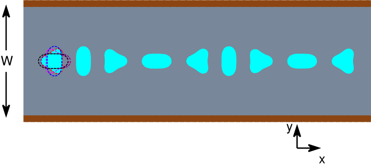
Figure 2: (Color online) Snapshots of an axially moving swimmer over time ($W=10.0R_{0}$). The dashed profiles show a complete period $T_{s}$ of deformation and then a few shapes are represented over a time of the order of $170T_{s}$. $\Gamma=0.085$, $S=10$.

In physical units the average velocity of the swimmer will be defined as $\langle V\rangle=[X_{c}(t+T_{s})-X_{c}(t)]/T_{s}$ (this is the net displacement of the center of mass over one cycle divided by the stroke cycle period). We will define the dimensionless instantaneous velocity as $\bar{V}=VT_{s}/R_{0}$. Its average over one swimming cycle is defined as $\langle\bar{V}\rangle=\bar{X}_{c}(t+T_{s})-\bar{X}_{c}(t)$, where $\bar{X}_{c}=X_{c}/R_{0}$.

Figure 3 shows the center of mass of the swimmer, $\bar{X}_{c}(t)$, undergoing a periodic oscillation in the axial direction as shown in (a). A first observation is that for $C$ not too large (from $C=0.01$ up to $C=0.71$), the amplitude of the oscillation increases with confinement. The slope of the curves $\bar{X}_{c}(t)$ also increase with $C$, indicating an enhancement of migration speed upon increased confinement. The increase of oscillation amplitude with $C$ (for not too large $C$) is already an interesting indication that the swimmer takes advantage of the walls to enhance its migration speed.

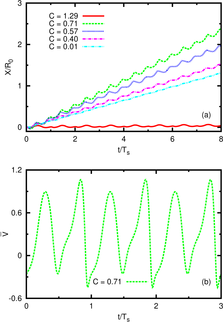
Figure 3: (Color online) (a) An axially moving amoeboid swimmer undergoes a periodic oscillation in the axial direction ($x$ direction) of the channel as a function of time. From strong to weak confinements, the corresponding oscillatory motions are represented by different types of colorful lines. (b) Velocity of an axially moving swimmer as a function of time. $\Gamma=0.085$, $S=10$.

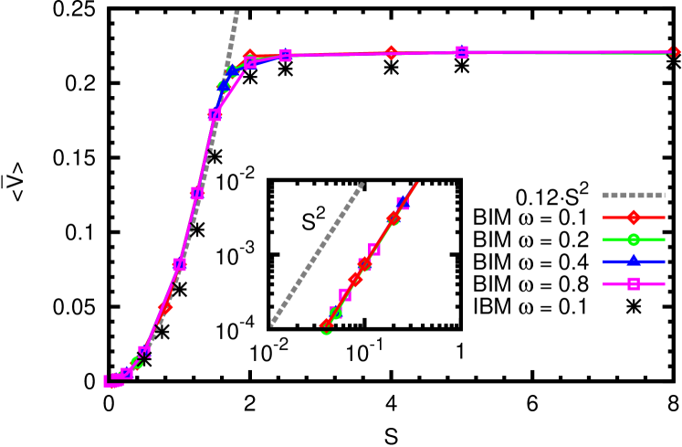
Figure 4: (Color online) (a) The time-averaged velocity magnitude attains a plateau with the increasing dimensionless amplitude of active forces $S$; $\Gamma=0.085$ and $C=0.5$. The inset shows the scaling $S^{2}$ (grey dashed line) in a $\log-\log$ plot. The stars are data obtained by IBM, the other data are obtained by BIM.

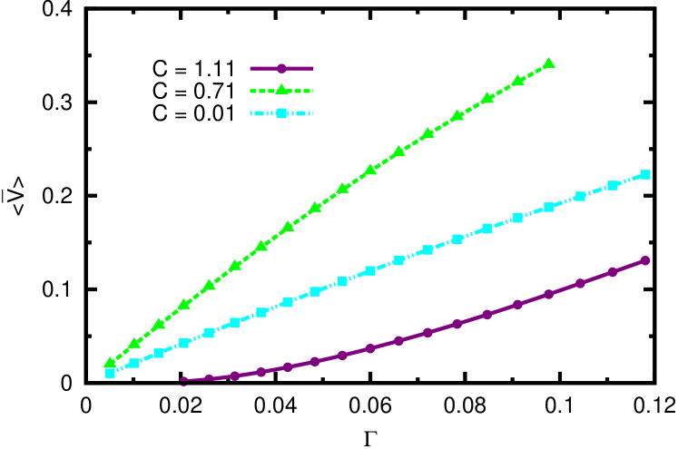
Figure 5: (Color online) In different confined regions, the linear and nonlinear relations between the excess length $\Gamma$ and the velocity magnitude $\bar{V}$ are calculated; $S=10$.

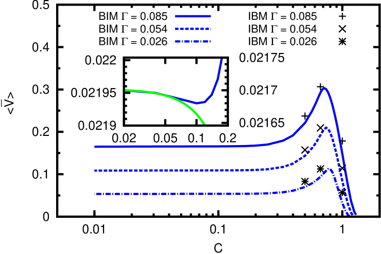
Figure 6: (Color online) Time-averaged velocity magnitudes as a function of $C$ in $\log$ scale for different $\Gamma$s. The data represented by the solid lines are calculated by BIM, while the data represented by symbols are calculated by IBM; $S=10$. The inset shows a zoom for weak confinement with $\Gamma=0.010$ showing a weakly decreasing velocity (scale on the left side) and its comparison with the analytical theory in green (see also section V), with the scale on the right side. The full numerical analysis and the analytical result agree quite well as long as the confinement is weak enough, in line with the assumption used to find the analytical solution.

Fig. 3 (b) shows that the instantaneous velocity changes during three deformation stroke periods. The negative velocity is induced by the confining walls; in the unconfined case the velocity always remains positive Farutin et al. (2013).

IV.1 Scaling of the swimming velocity with the force amplitude

Due to the linearity of the Stokes equations, one may expect that the velocity of the swimmer scales linearly with the force. This has been adopted as a hypothesis in several studies where the swimmer is modeled as rigid body. Typical examples are the medeling of E. coli Lauga et al. (2006); Berke et al. (2008), Bacillus subtilis Sokolov and Aranson (2009) (examples of the so-called pushers), and Chlamydomonas (an example of puller) Drescher et al. (2009); Guasto et al. (2010); Kantsler et al. (2013). In the present study the relation between the velocity and the force is extracted a posteriori. We find that the velocity is a nonlinear function of the force amplitude. We have defined in equation (9) a set of three dimensionless parameters. Our goal in this section being to discuss the effect of the force amplitude, we set $\Gamma$ and $C$ to constant values. The physical (i.e. not the dimensionless) average velocity over a swimming cycle is given, from dimensional analysis, by the relation

$$\langle V\rangle\sim{R_{0}\over T_{s}}G(S).$$ (13)

where $G(S)$ is a scaling function, unknown for the moment. Let us first provide some bases for the behavior of $G(S)$ using physical intuition. An obvious guess is that for a large $S$, $\langle V\rangle$ should be independent of the force amplitude. Indeed, recall that $S$ can be written as $S\sim T_{s}/T_{c}$. This is the ratio between the stroke period and the shape adaptation time. A large $S$ (i.e. a large force) implies that the swimmer attains its saturated shape (in response to applied forces) in a shorter time than the stroke time interval. In other words, further increasing the force amplitude will hardly change the sequence of shapes explored by the swimmer during one stroke cycle. This increase of $A$ does not promote faster swimming, only a faster adaptation time. Indeed, in the Stokes regime time does not matter - only the configuration is important. Therefore, the speed should attain a plateau at large $S$. Our numerical simulation clearly shows this behavior (Fig. 4). We can thus conclude that for large $S$, $\langle V\rangle\sim\omega R_{0}$. The velocity is thus solely determined by the stroke frequency.

The situation is less obvious for small $S$, the limit in which the force configuration changes in time faster than the shape adaptation. Increasing $S$ (but remaining in the small range limit) means the shape has more time to adapt (though not yet fully), resulting in a faster and faster motion since the shape, for each increase of $S$, will be deformed more and more until saturation (when the force is large enough). The first natural expectation would have been that we would see a linear relationship between velocity and force, but this naive expectation does not comply with the numerical finding. Our results show a quadratic behavior. A qualitative argument in favor of this behavior is the following: if $A$ is small, it is legitimate to perform a perturbation theory in powers of $A$. The swimmer deformation (due to active force $F_{a}(\alpha,t)$ given by equation (4)) is proportional to leading order to $F_{a}$, as is the swimmer velocity. Averaging the velocity over a cycle gives zero, since $F_{a}(\alpha,t)$ is proportional to a superposition of $\cos(\omega t)$ and $\sin(\omega t)$. Therefore the first non-vanishing contribution is quadratic in $F_{a}$, leading to a quadratic dependence on $A$. Quadratic behavior was also recently reported for the three-bead swimmer Pande and Smith (2015). However, no saturation regime was shown in that paper.

In summary, the velocity of the swimmer behaves as

$$\langle V\rangle\sim\left\{\begin{array}[]{ll}{(R_{0}/T_{s})}S^{2}={R_{0}T_{s}A^{2}/\eta^{2}}&(S\ll 1),\\ {R_{0}/T_{s}}&(S\gg 1).\end{array}\right.$$ (14)

Figure 4 shows the full nonlinear behavior obtained from the numerical solution which is in agreement with the above scalings. Note that the velocity behaves for small force as $1/\eta^{2}$, which is distinct from the classical Stokes result where the velocity is $\sim 1/\eta$. This behavior is amenable to experimental testability (provided that the swimmer operates at a fixed given force when viscosity is varied). It is not however clear if the condition of $S\ll 1$ is abundant or not in the amoeboid swimming world. It is thus of great importance to conceive of artificial amoeboid swimmers that could be monitored in order to scan the whole range of $S$ so as to permit tests of the above scaling relations.

IV.2 Velocity of the swimmer as a function of confinement and excess length

We have determined the velocity as a function of the deflation of the swimmer, a deflation characterized by the excess length $\Gamma$. Quasi-linear and nonlinear relations between the center of mass’ velocity magnitude $\bar{V}$ and the excess length $\Gamma$ are found depending on confinement, as shown in Fig. 5. We expect that the more the swimmer is deflated the larger its velocity. Indeed, the deformation amplitude of the swimmer increases with $\Gamma$, which thus implies a higher speed. From Fig. 5, it is found that the exponent for weak confinement is almost $1$ (shown by a cyan line in Fig. 5), and agrees with the study for a completely unbounded swimmer Farutin et al. (2013). However, as confinement increases the picture is more complex: we have, at small $\Gamma$, a power law with exponent lower than $1$ (green line) in the intermediate confinement regime, and an exponent higher than 1 in the case of strong confinement (shown by a purple line in Fig. 5).

A prominent property we have recently reported on Wu et al. (2015) is the velocity’s non-monotonous behavior with confinement $C$. The results are summarized in Fig. 6, where we compare the outcome of the two numerical methods showing good agreement. Both methods show a maximum in the $\langle\bar{V}(C)\rangle$ curve.

V On the non monotonous behavior of the swimmer velocity as a function of $C$

Once we have clarified the role of the force amplitude in the swimming speed, we would like to discuss the behavior of the velocity as a function of confinement (Fig.6) . We will first provide a brief summary of wall effects reported so far in the literature before discussing our results. The fact that the wall enhances motility is reported in several papers Felderhof (2010); Jana et al. (2012); Zhu et al. (2013); Bilbao et al. (2013); Ledesma-Aguilar and Yeomans (2013); Acemoglu and Yesilyurt (2014); Liu et al. (2014). However, we must stress, as we found, that this is not always true. A close inspection shows that at weak confinement the velocity may first decrease and then increase; see below. It must be noted that besides swimming based on cilium or flagellum activity, there has been also a large number of studies devoted to amoeboid swimming bounded by walls in the biological literature, as discussed below.

Felderhof Felderhof (2010) has reported on the fact that confinement enhances the speed of the Taylor swimmer. Later, Zhu et al. Zhu et al. (2013) considered the squirmer model to show that speed decreases with confinement when the squirmer surface deformation is tangential only. If on the contrary normal deformation is also allowed, the speed increases with confinement. Liu et al. Liu et al. (2014) reported on another model, namely a helical flagellum moving in a tube and found that, except for small tube radii, the swimming speed for a fixed helix rotation rate increases monotonically with confinement. Acemoglu et al.Acemoglu and Yesilyurt (2014) adopted a similar model but, besides the flagellum, their swimmer is endowed with a head. They found in this case an opposite tendency: the speed decreases with confinement. Bilbao et al.Bilbao et al. (2013) analyzed a model inspired by nematode locomotion by simulation and found that walls enhance the speed. Ledesma et al.Ledesma-Aguilar and Yeomans (2013) treated a dipolar swimmer bounded both by rigid or an elastic tube and obtained a speed enhancement due to walls.

The effect of confinement on cell motility is a also a major field of research in biological literature. Several in vitro devices have been set up in order to analyze this issue for different kinds of cells. For example, some cancer cells use a mesenchymal motion when unconfined, while under confinement (and in the absence of focal adhesion) they can switch to a fast amoeboid locomotion Liu et al. (2015). The enhancement of the speed under confinement in this case is likely to be a complex phenomenon, since it is not only due to a pure hydrodynamical phenomenon, but to an internal cellular transition of mode locomotion. It will be interesting to include in our model in the future inclusion several competing modes to check if one mode prevails over another when changing the external environment. speed, pointing to the complexity of the effect of the walls.

V.1 The flow field

In this section we would like to provide a qualitative picture regarding the increase of swimming velocity with increased confinement. A starting point for the qualitative argument describes the swimmer as grasping the wall to enhance its motion. When the confinement is too strong, the swimmer can not fully deploy its shape and therefore a collapse of the velocity is expected. In actuality, the situation is more subtle, as will be discussed below.

Let us analyze in some details the flow pattern and dissipation around the swimmer to provide some hints toward understanding the basic mechanisms. We shall then point out some analytical results that show the complex nature of the phenomenon. Fig. 7 shows the flow pattern around the swimmer. It consists of two swirls which lie inside the AS. The flow pattern has a structure of a source dipole. A source in 2D creates a flow which is inversely proportional to distance in 2D, meaning that the source dipole has an asymptotic behavior which is inversely proportional to the square of the distance.

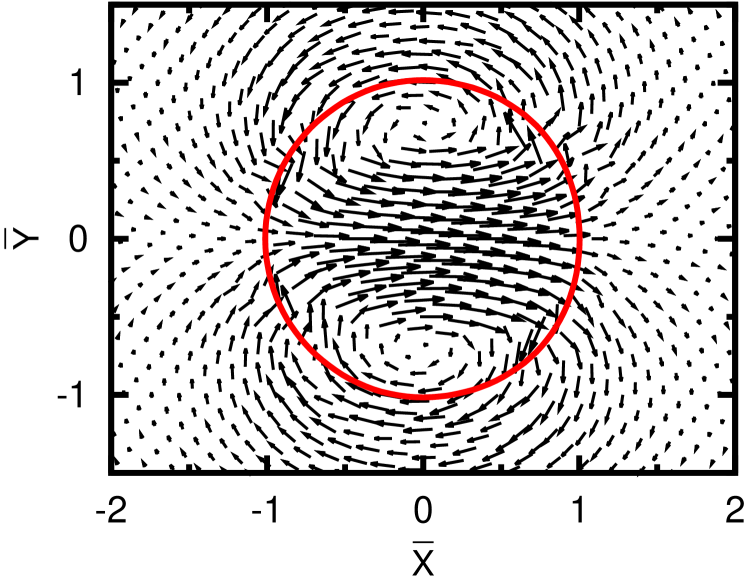
Figure 7: (Color online) The time-averaged shape of the swimmer over one swimming cycle and its corresponding velocity field. $C=0.40$, $\Gamma=0.085$, $S=10$.

V.2 Dissipation function

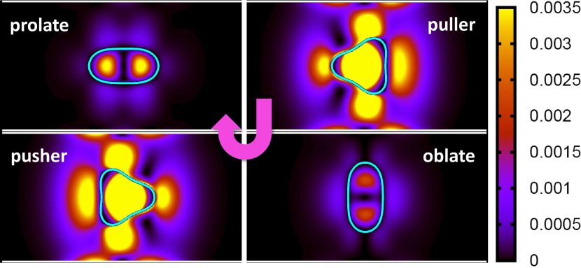
Figure 8: (Color online) A series of instantaneous dissipation distributions during one complete swimming stroke. Color shows the intensity of dissipation density, and the blue represents the contour of the swimmer. Swimming direction goes to the right. An amoeboid swimmer combines pusher and puller behavior during one deformation period. $C=0.40,\Gamma=0.085$, $S=10$.

The instantaneous intensity of dissipation density is given by:

$$\Psi_{v}=\sigma_{ij}\frac{\partial u_{i}}{\partial x_{j}}=2\eta\epsilon_{ij}\epsilon_{ij},$$ (15)

where $\sigma_{ij}=-p\delta_{ij}+2\eta\epsilon_{ij}$, $\epsilon_{ij}=1/2(\partial_{j}u_{i}+\partial_{i}u_{j})$, and repeated subscripts are to be summed over. The expression reads explicitly in $x-y$ coordinates as

$$\Psi_{v}=2\eta\left[\left(\frac{\partial u_{x}}{\partial x}\right)^{2}+\left(\frac{\partial u_{y}}{\partial y}\right)^{2}\right]+\eta\left(\frac{\partial u_{x}}{\partial y}+\frac{\partial u_{y}}{\partial x}\right)^{2}.$$ (16)

The rate of work (output power) performed by AS is instantaneously equal to the rate of total energy dissipation in the fluid. The hydrodynamic interactions between the swimmer and the walls are illustrated by a series of instantaneous dissipation patterns produced during the process of one complete AS stroke in Fig. 8. The corresponding instantaneous configurations of a wall-confined amoeboid swimmer are plotted by a closed cyan solid line (see Fig. 8), from which we can clearly observe that the swimmer uses the wall as a support on which much of the work is performed (grasping). The instantaneous dissipation shows two-arm-like distributions extended to the walls during the puller and pusher states, so that one can intuitively understand that the swimmer’s speed is increased by extended arm-like dissipation structures creating hydrodynamical friction with the walls.

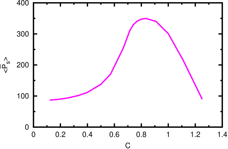
Figure 9: (Color online) The time-averaged power consumption $\langle{\bar{P}_{s}}\rangle$ as a function of $C$ for $\Gamma=0.085$, $S=10$.

We define a time-averaged power consumption (rate of work) as

$$\langle P_{s}\rangle = \frac{1}{T_{s}}\int^{T_{s}}_{0}\oint_{\partial\Omega}\left[{\mathbf{F}}(s)\cdot{\mathbf{u}}(s)\right]dsdt$$ (17)

$$= \langle\oint_{\partial\Omega}\left[{\mathbf{F}}(s)\cdot{\mathbf{u}}(s)\right]ds\rangle,$$

where $T_{s}$ is a swimming period. A dimensionless average power is defined as $\langle{\bar{P}_{s}}\rangle=\langle P_{s}\rangle T_{s}^{2}/(\eta R_{0}^{2})$. Fig. 9 shows the dimensionless time-averaged power of the active forces. Power consumption $\langle{\bar{P}_{s}}\rangle$ attains a maximum at a confinement which is close (but not equal) to the confinement at which a maximum velocity is obtained (Fig. 6). In the strongly confined regime, the power rapidly decreases because the deformation amplitude is strongly reduced by the wall constraints: the swimmer is in principle able to deploy a larger amplitude but the rigid walls block this tendency. This is supported by a recent experiment Nosrati et al. (2015) according to which the flagellar wave amplitude of bull sperm in the extremely confined condition is so strongly suppressed that they have to adopt a slithering motion to swim along a rigid surface. The swimming velocity of bull sperm becomes slower and slower.

Note finally that an analytical study (a detailed report of which we make elsewhereFarutin et al. (2016)) performed at weak confinement has allowed us to extract the swimming velocity as a function of confinement:

$$\langle{V}\rangle=\frac{5\pi\Gamma R_{0}}{3\sqrt{6}T_{s}}-0.12C^{2}\frac{\pi\Gamma R_{0}}{T_{s}}+O(C^{3}\Gamma)+O(\Gamma^{3/2}).$$ (18)

The first term corresponds to the purely unconfined case and we capture the same dependence with $\Gamma$ as in the 3D case Farutin et al. (2013). The second term is the first contribution of confinement to the swimming speed, and is negative, meaning that at very small confinement the wall reduces the swimming speed. This is visible in the inset of Fig. 6. This remark shows clearly that the effect of the walls is not quite obvious.

VI Efficiency of swimming

In this section we wish to investigate the notion of efficiency. We will first adopt a widely used definition of swimming efficiency, which is the ratio of the least power required to drag (or pull) the swimmer along the axis at its time-averaged speed $\langle V\rangle$ (the physical one, not the dimensionless one) over the actual time-averaged output power $\langle P_{s}\rangle$ generated by the swimmer Lighthill (1975); Purcell (1997); Becker et al. (2003). Here we define a dimensionless $2$D efficiency $\Pi_{1}$ as

$$\Pi_{1}=\frac{\eta\langle V\rangle^{2}}{\langle P_{s}\rangle},$$ (19)

where $\langle V\rangle$ is the average physical velocity. ¨Figure 10 shows that the optimal swimming occurs at the transition point where the velocity as a function of the applied force saturates (see Fig.4). The qualitative behavior of the efficiency curve can be explained as follows. When $S$ is small (small force, before the plateau is reached in Fig.4) the stroke dynamics is so fast that it does not allow to the swimmer to attain its saturated shape, and the swimmer loses efficiency. If $S$ is too large, this does not bring any benefit since the swimmer reaches its saturated shape too quickly, and does not gain in efficiency by a further increase of force.

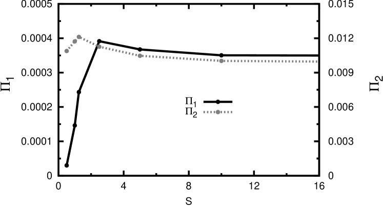
Figure 10: (Color online) The two efficiencies $\Pi_{1}$ and $\Pi_{2}$ as functions of $S$. $C=0.5$ and $\Gamma=0.085$.

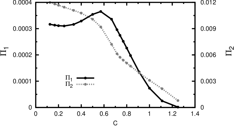
Figure 11: The efficiencies ${\Pi}_{1}$ and $\Pi_{2}$ as functions of $C$ for $\Gamma=0.085$, $S=10$.

It is also worthwhile to examine the efficiency as a function of the strength of confinement $C$. Using the definition above, we find that the maximum efficiency occurs at a confinement of $C\simeq 0.6$, which is different from that corresponding to the maximum speed (Fig. 6, $C\simeq 0.75$). The efficiency ${\Pi}_{1}$ first gradually increases and then decreases rapidly after the optimal point.

A second swimming efficiency considered in literature is noteworthy. Defined as $\sim\langle V\rangle/\langle P_{s}\rangle$ Shapere and Wilczek (1987); Koiller and Delgado (1998), it seems to be suitable for small deformations since for small deformations, $V\sim\Gamma$, then $P_{s}\sim\Gamma$; the efficiency is independent of $\Gamma$. This definition of efficiency is not dimensionless. We adopt here a dimensionless form given by

$$\Pi_{2}=\frac{\eta\omega R_{0}\langle V\rangle}{\langle P_{s}\rangle}.$$ (20)

The corresponding results are shown by the grey dashed dotted line in Fig.9 and Fig. 11, from which no optimal value for a special confinement is found, in contrast to the definition (19). This example clearly highlights the main difference between the two definitions. It also points to the fact that there seems to be no straightforward definition of a suitable efficiency (if any).

VII Various dynamical states of the swimmer: from straight trajectory to navigation

In this section we present the rich panel of behaviors manifested by the AS. We shall see that the AS can settle into a straight trajectory, can navigate in the channel with a fixed amplitude in a symmetric or asymmetric way, or can even crash into the wall. The adoption of one or another regime depends on various conditions, and especially on the force distribution and on the degree of confinement. One extra degree of complexity that is unique to the AS is the fact that the nature of the swimmer (puller, or pusher) is not an intrinsic property of the swimmer itself, but depends on the environment (say on confinement). Before discussing our results, we would like first to put our work in the context of swimmers in general.

Zhu et al. Zhu et al. (2013) adopted the squirmer model which can be set to be a pusher, a puller or neutral, by the appropriate choice of parameters. They find that a pusher crashes into the wall, a puller settles into a straight trajectory, and a neutral swimmer navigates. However, the navigation amplitude depends on initial conditions: it is not a limit cycle, but an oscillator, akin to what happens for Hamiltonian systems.

Najafi et al. Najafi et al. (2013) used a three-bead model and reported on the navigation possibilities of the swimmer. It was not clear in that study if the navigation amplitude was dependant or not on initial conditions. Actually, no conclusion on whether or not the navigation period reaches a final given value was made.

Since the nature of the swimmer seems to play an important role, it is interesting to first define this notion and analyze it for our system before presenting the main results.

VII.1 Swimmer nature evolution

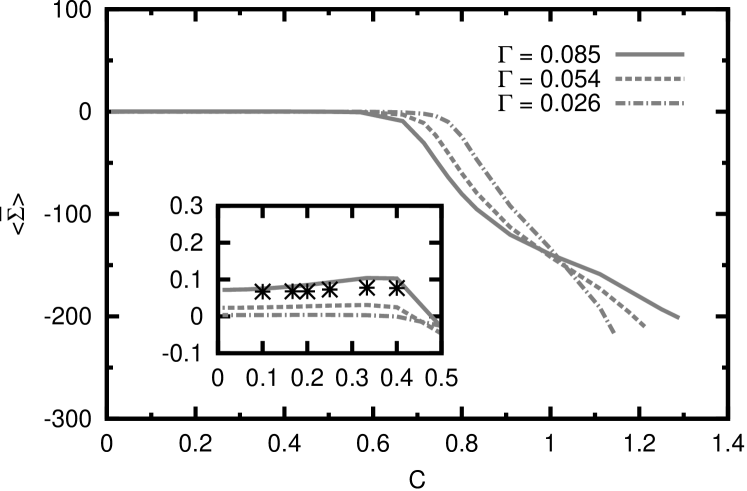
Figure 12: (Color online) Time-averaged stresslet $\langle\bar{\Sigma}\rangle$ as a function of confinement $C$ showing the transition from pusher to puller. Different lines refer to an axially moving swimmer and stars to a symmetrically navigating swimmer. Inset shows a zoom for small $C$ in order to show the confinement at which the pusher-puller transition occurs. $S=10$.

Swimmers are classified as pushers, neutral swimmers or pullers, depending on the sign of the stresslet. This notion is defined on the average over one cycle. During half a cycle a swimmer may behave as a puller while during the second half as a pusher. What matters here is the average nature. For example, Chlamydomonas Reinhardtii Drescher et al. (2009); Guasto et al. (2010); Garcia et al. (2011); Kantsler et al. (2013), switches from a puller to a pusher over one cycle, but is a puller on the average over one swimming cycle. The nature of our swimmer will also be defined by an average over one cycle. The interesting feature which emerges here is that our swimmer may behave as a pusher on the average, but if the confinement changes it switches, on average, to puller behavior. In other words, the swimmer seems to adapt its nature to the environment. In the far-field approximation, the first contribution (in a multipolar expansion) to the velocity field is governed by a term of the form $\Sigma_{ij}=\oint F_{i}r_{j}ds$. Exploiting symmetry of the swimmer (axial symmetry) we can write that the far field is, to leading order, proportional to $\bar{\Sigma}=(\Sigma_{xx}-\Sigma_{yy})/(\eta R_{0}^{2}/T_{s})$, which we will call a (dimensionless) stresslet hereafter. The instantaneous type (pusher or puller) of an AS can be identified by the sign of the instantaneous stresslet: (${\bar{\Sigma}}>0$ indicates a pusher and ${\bar{\Sigma}}<0$ indicates a puller). As already pointed out earlier Farutin et al. (2013) our swimmer observes, in the course of time, an entangled puller-pusher state. We could split the swimming cycles into 4 intervals. In the first interval the swimmer behaves as a pusher, followed by an interval where it behaves as a mixed pusher-puller state, a third interval in which it behaves as a puller, and finally a fourth interval in which it assumes a mixed state (see also Fig.8). Another possible way of characterizing our swimmer is to determine its nature on average over one swimming cycle. The dimensionless average stresslet is given by ${\langle\bar{\Sigma}\rangle}=(\int_{0}^{T_{s}}\bar{\Sigma}dt)/T_{s}$ (the average over one deformation period $T_{s}$). Figure 12 shows this quantity as a function of confinement. The swimmer behaves as a pusher for $C\lesssim 0.5$, and as a puller for $C>0.5$. The efficiency shown in Fig. 11 shows an optimum for $C\sim 0.6$ which is close to the pusher-puller transition.

VII.2 Navigation and symmetry-breaking bifurcation

In the weak confinement regime (where the swimmer is a pusher on average, see Fig. 12) it is found that the straight trajectory is unstable in favor of navigation, and that the navigation amplitude is a function of confinement independent of initial conditions. This is confirmed by the results of both numerical methods (BIM and IBM). Snapshots are shown in Fig. 13 where one can observe ample navigation of the swimmer. Typical evolution of the $Y_{c}$ position as a function of time is shown in Fig. 13. This curve shows a large scale navigation period with a small scale structure associated with the strokes of the swimmers. Let us define the navigation amplitude $\Delta Y$ as the difference between the maximum of $Y(t)$, $Y_{t}$, and the minimum of $Y(t)$, $Y_{b}$, $\Delta Y=Y_{t}-Y_{b}$ and plot this amplitude as a function of confinement $C$ (Fig. 14). We see that the amplitude decreases with $C$. The swimmer does not crash into the wall, in contrast with the squirmer model studied in Ref. Zhu et al. (2013) . Indeed, we find that the navigation amplitude reaches saturation after some time. The navigation mode also survives when the swimmer behaves as a puller on average, and does not settle into a straight trajectory, unlike the finding in Ref. Zhu et al. (2013). In Fig. 14 the domains of puller and pusher are shown.

The navigation mode undergoes an instability at a critical confinement $C\simeq 0.8$ (where it behaves as a puller) in favor of an asymmetric motion where the swimmer moves closer to one of the two walls. The amplitude $Y_{c}(t)$ of the center of mass is shown in Fig. 15. The center of mass shows an oscillation which is determined by the stroke frequency, in contrast to in the navigating mode which, apart from the small scale oscillation due to the strokes, develops large scale oscillations of the position. Figure 15 shows the trajectory of the asymmetric swimmer. The overall behavior is summarized in Fig. 16. There we show the average position of the center of mass as a function of confinement $C$. For small $C$, the center of mass position averaged over a navigation period is zero. There is a spontaneous symmetry-breaking bifurcation at $C\sim 0.8$ where the swimmer moves towards either of the two walls. In this regime the center of mass of the swimmer shows temporal oscillations which are asymmetric (lower rectangle in the figure). The bifurcation is supercritical (albeit quite abrupt). At $C=1.04$, the average position of the center of mass crosses zero.

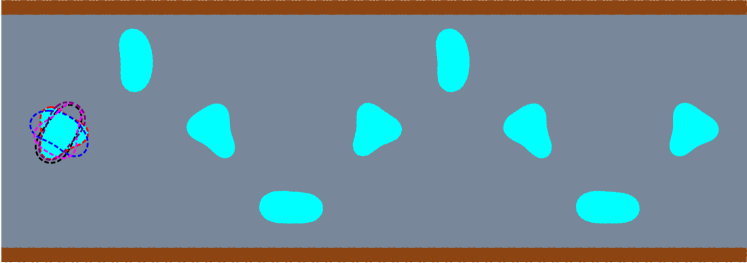
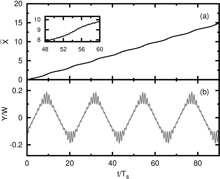
Figure 13: (Color online) Top: Snapshots of a navigating swimmer over time ($W=10.0R_{0}$). The dashed profiles show a complete period $T_{s}$ of deformation. Few shapes are represented over two navigation periods $T$ of the order of $240T_{s}$. $\Gamma=0.085$, $S=10$. Bottom: A navigating amoeboid swimmer in the channel undergoes periodic oscillations in both ${x}$ (a) and ${y}$ (b) directions. The inset in (a) shows the short periodic oscillations due to strokes which are superimposed on the long periodic oscillations due to the navigation. $C=0.50,\Gamma=0.085$, $S=10$.

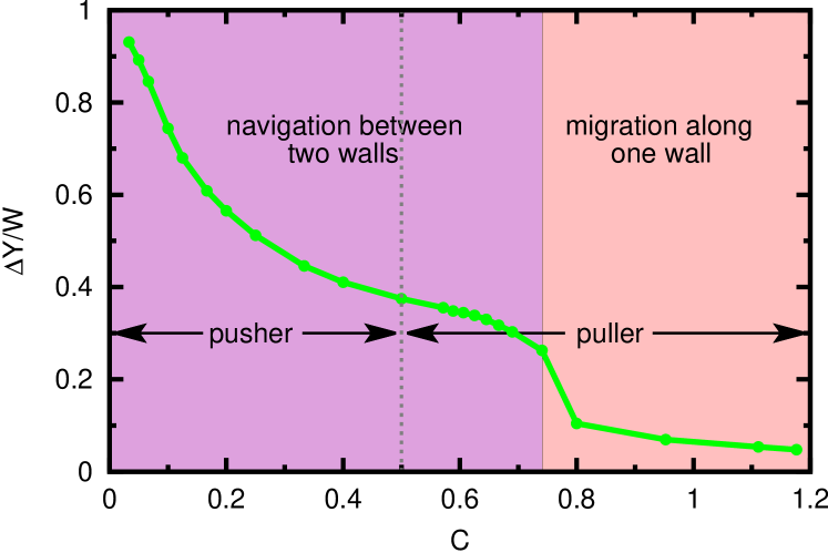
Figure 14: (Color online) The amplitude of navigation as a function of confinement $C$. $\Gamma=0.085$, $S=10$.

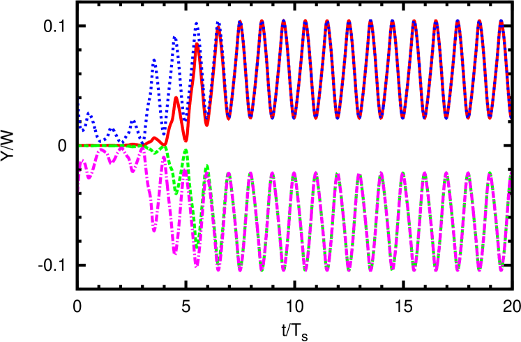
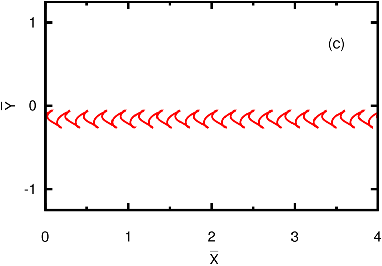
Figure 15: (Color online) Top: The vertical position of center of mass $Y_{c}$ as a function of time $t$ showing the symmetry breaking bifurcation. Different colors represent different initial positions. Bottom: trajectory of the asymmetric swimmer. $\Gamma=0.085$, $S=10$, $C=0.8$.

VII.3 Ability of scanning space

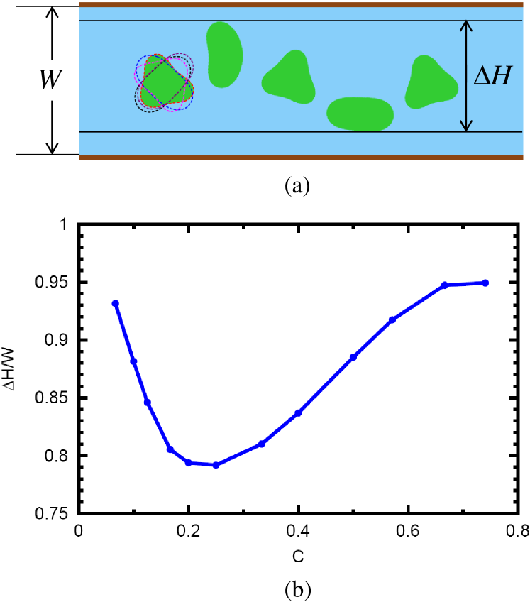
Figure 17: (Color online) (a) The definition of height difference $\Delta H$ scanned by a navigating swimmer. (b) The scanned space for different confinements ($\Gamma=0.085$, $S=10$).

We were interested in analyzing the swimmer’s ability to scan the available space. We measured the highest membrane point of the swimmer in the channel, calling it $H_{t}$ and the lowest membrane point, calling it $H_{b}$. The difference $\Delta H=H_{t}-H_{b}$ is a direct measure of space scanning by the swimmer. In Fig. 17 (top panel) we provide a schematic representation of this measure. The lower panel provides the numerically computed scanning amplitude as a function of confinement. It is found that the navigating mode can explore between about $80\%$ and $95\%$ of the available lateral space.

VII.4 Crashing into the wall and settling into a straight trajectory

As stated above it has been reported Zhu et al. (2013) (by adopting a squirmer model) that the pusher crashes into the wall while a puller settles into a straight trajectory. This contrasts with our finding presented above. We have thus attempted to investigate this question further in order to clarify the situation. We find that the type of trajectory depends strongly on the strength of the stresslet $\bar{\Sigma}$ and the strength of a linear combination $D$ of dimensionless force quadrupole $\bar{\Sigma}_{2}$ and source dipole $\bar{\Delta}_{2}$ Wu et al. (2015). A weak pusher or puller means that the stresslet $\bar{\Sigma}^{2}\ll\bar{V}\bar{D}$ Wu et al. (2015), where $\bar{D}$ is the dimensionless force quadrupole strength. For example, if the swimmer is a weak pusher, we have navigation and symmetry-breaking as presented above. On the contrary, if the pusher is strong enough we also find that the swimmer has a tendency to crash into the wall. Similarly, if the puller is strong enough we find that the swimmer settles into a straight trajectory with $Y_{c}(t)=0$ if the swimmer is at the center of the channel, or with $Y_{c}(t)$ periodic in time due to strokes if the swimmer at some distance from the center, as is the case in Fig. 15, bottom.

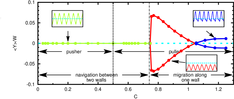
Figure 16: (Color online) Average position along $y$ as a function of confinement. $\Gamma=0.085$, $S=10$.

In order to have a swimmer with a large enough stresslet, we can modify the force presented in section II.1 in the following way

$${\mathbf{F}}=2[\sin(\omega t)\cos(3\alpha)-(\beta+\cos(\omega t))\cos(2\alpha)]{\mathbf{n}}$$ (21)

where we recall that $\alpha=2\pi s/L_{0}$ ($s$ is the arclength and $L_{0}$ the perimeter), or

$${\mathbf{F}}=2[(-\beta+\sin(\omega t))\cos(3\alpha)-\cos(\omega t)\cos(2\alpha)]{\mathbf{n}}.$$ (22)

Setting $\beta=0.5$ in equation (21) and (22) gives a puller and a pusher, respectively.

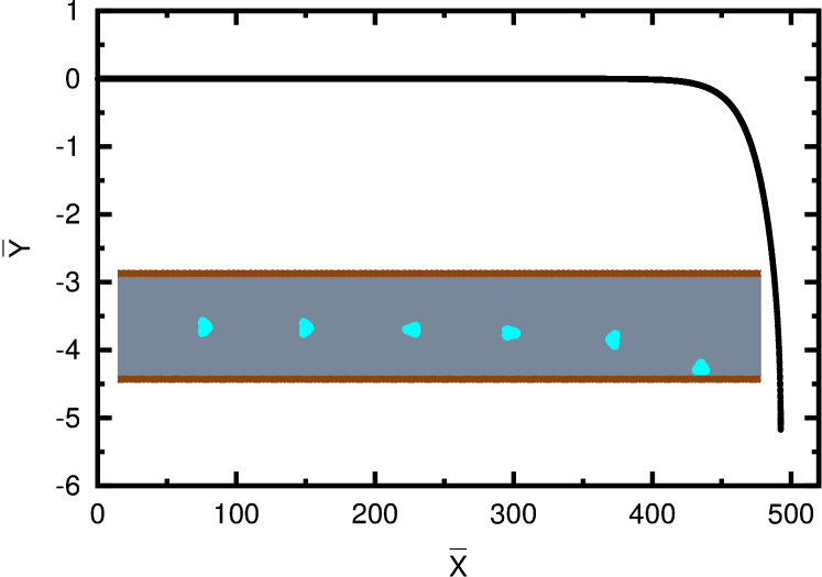
Figure 18: (Color online) A trajectory showing a swimmer crashing into the wall. $\Gamma=0.054$, $S=1$, $C=0.167$.

Fig. 18 shows a typical trajectory for the case where the strong pusher crashes into the wall. We also provide the corresponding values of the stresslet. It would be interesting in the future to make a more detailed analysis of this problem in order to determine the critical amplitude of the stresslet above which we have a transition from navigation to crashing/settling into a straight trajectory. In contrast, a strong puller is found (Fig. 15, bottom) to move along the channel. The center of mass undergoes small vertical oscillation due to shape deformation when the swimmer selects an off-centered trajectory.

VIII Discussion and perspectives

The current work presents a systematic study of the hydrodynamics of microswimming by shape deformation (amoeboid swimming) in a planar microfluidic channel. By studying the coupling of shape change and wall interaction, we discovered several new features of microswimming. Let us highlight the new features discovered here, and recall some facts we reported on recently.

• In agreement with our recent report Wu et al. (2015) we confirm that the nature (pusher or puller) of the swimmer is not an intrinsic property. Several swimmers may have an instantaneous nature which changes over time. For example, Chlamydomonas Reinhardtii  Drescher et al. (2009); Guasto et al. (2010); Garcia et al. (2011); Kantsler et al. (2013) is on the average (average over one swimming cycle) a puller, albeit it has two temporal phases where it behaves like a puller or a pusher. We also found here that the amoeboid swimmer can exhibit a pusher or a puller behavior at a given time; however, the stresslet, averaged over one cycle, can change under the influence of external factors such as confinement, unlike other swimmers studied so far. For example, by changing the environment (like confinement) an amoeboid swimmer which is a pusher on the average, becomes a puller (or vice versa) when external parameters are changed.

• The straight trajectory of the swimmer can become unstable in favor of navigation. Navigation has been reported for other swimmers in two different studies Najafi et al. (2013); Zhu et al. (2013). However, in the study using a three-bead model Najafi et al. (2013) there is no conclusion about the final amplitude of navigation (it increases monotonously with time), while in the study using a squirmer as a model Zhu et al. (2013) navigation was found for a neutral swimmer only, and the navigation amplitude depended on initial conditions. Here, in contrast, we found that navigation can occur for pushers (a weak enough pusher) as well as for neutral swimmers. For pushers we find that the amplitude is fixed, in that it does not depend on initial conditions.

• The confinement was found to enhance the swimming speed in several previous studies Felderhof (2010); Jana et al. (2012); Zhu et al. (2013); Bilbao et al. (2013); Ledesma-Aguilar and Yeomans (2013); Acemoglu and Yesilyurt (2014); Liu et al. (2014). Here also we reach the same conclusion, but with the specification that monotonous behavior (even in the weak confinement regime) is not a general tendency, so the reverse can also sometimes occur (Fig. 6). This points to the fact that this question should be more carefully considered.

• In a previous study Zhu et al. (2013) it was reported that a pusher crashes into the wall and a puller settles into a straight trajectory. Here we have reported that this is not a general result: a pusher can also undergo navigation with a well-defined amplitude.

• The swimming speed is found to be quadratic with the force amplitude and then tends towards a plateau at large enough amplitude. The quadratic behavior is shared with that of a three-bead swimmer Pande and Smith (2015), but no regime with a plateau was reported there. We believe that a modified three-bead model having a nonlinear spring with saturation (like with the so-called FENE model) should capture the plateau behavior.

Although the present study provides a first route for the modeling of amoeboid swimming, several other questions deserve future consideration in order to capture a more realistic picture of swimming cells. In the present work, we assumed the membrane to be a simple phospholipid envelope whereas real cells are endowed with a cytoskeleton and a nucleus making the deformations more difficult. From equation (14), one can extract an order of magnitude of the active force of about $0.01$ pN (using typical quantities Liu et al. (2015) for a $10\mu$m cell diameter, a migration velocity of $10\mu$m/min, a water-like medium viscosity and a swimming cycle of characteristic time $1$ min). This force is smaller than the available force in a real cell. It will be of great importance to include the cell cytoskeleton in modeling for better comparison with experimental systems. For the sake of simplicity we have also considered a simple periodic function for the active forces. Real observations of cell motion Lämmermann and Sixt (2009); Liu et al. (2015) point to more complex shape dynamics. Similar complex motions could be reproduced by assigning a complex time-dependent force distribution (including higher harmonics). It will be interesting in the future to use experimental data and, by solving an inverse problem, extract the active forces (both in space and time) to be used in our model for a more realistic analysis.

Another future issue is the study of the wall compliance effect Ledesma-Aguilar and Yeomans (2013). Indeed, many eukaryotic cells in vivo (e.g. cells of the immune system, cancerous cells…) move in soft tissues where cells are often in interstices, in between other cells and extracellular matrix. Therefore, the confinement is not fixed in time but varies in response to stresses created by the cells. A basic representation of this effect could be had by considering bounding walls of a certain compliance. Flexible walls can promote swimming in the strong confinement regime by allowing larger amplitude of deformation of the swimmer than rigid walls do. Another important issue is to study the collective behaviors. For example, during wound healing and cancer spreading (to name but a few examples) cells move in a concerted fashion. It would be thus important to analyze if collective behaviors could emerge from the study of multiple swimmers, such as special patterns, synchronization, and so on. Finally, in vivo cells move in complex visco-elastic materials, and it will be an important issue in the future to analyze AS in a complex medium. An interesting issue will be to analyze the motion of a cell surrounded by other cells representing tissues. For example, how the rheology or the visco-elatsic properties of the tissue affect the amoeboid motion, both for a single cell and for collective motions.

IX Acknowledgments

H.W. thank Prof. S. Jung (Virginia Tech) for the helpful discussion on the experimental details. C.M., A.F., M.T., and H.W. were supported by CNES and ESA. S.R. and P.P. acknowledge support from ANR. All the authors acknowledge the French-Taiwanese ORCHID cooperation grant. W.-F. H., M.-C.L., and C.M. thank the MoST for a support allowing initiation of this project.

Appendix : Total force and total torque of tension force are zero

We have seen from general considerations that if the energy does not depend on position in space, then the total associated forces and torque are automatically zero. For interested readers we briefly give here an explicit proof. In $2$D space, an amoeboid swimmer is represented by a $1$D closed contour. For the force this is quite obvious since that force can also be written as

$$\mathbf{F}^{\rm{ten}}=\frac{\partial(\zeta\mathbf{t})}{\partial s}$$

Therefore the integral over a contour is zero.

For the total torque $\mathbf{T}^{\rm{tot}}$ along the perimeter of amoeboid swimmer, we have:

$$\mathbf{T}^{\rm{tot}} = \oint_{\partial\Omega}\left[\mathbf{r}\times\mathbf{F}^{\rm{ten}}\right]\rm{d}s$$

$$= \oint_{\partial\Omega}\left[(x-X_{c})F^{\rm{ten}}_{y}-(y-Y_{c})F^{\rm{ten}}_{x}\right]\rm{d}s$$

$$= \oint_{\partial\Omega}\left[(x-X_{c})\frac{\partial(\zeta t_{y})}{\partial s}-(y-Y_{c})\frac{\partial(\zeta t_{x})}{\partial s}\right]\rm{d}s$$

$$= \oint_{\partial\Omega}\left[(x-X_{c})d(\zeta t_{y})-(y-Y_{c})d(\zeta t_{x})\right]$$

$$= \oint_{\partial\Omega}\left[-\frac{\partial(x-X_{c})}{\partial s}(\zeta t_{y})+\frac{\partial(y-Y_{c})}{\partial s}(\zeta t_{x})\right]\rm{d}s$$

$$= \oint_{\partial\Omega}[-t_{x}(\zeta t_{y})+t_{y}(\zeta t_{x})]\rm{d}s$$

$$= 0$$

References

- Lauga and Powers (2009) E. Lauga and T. Powers, Rep. Prog. Phys. 72, 096601 (2009).
- Saintillan and Shelley (2012) D. Saintillan and M. Shelley, J. R. Soc. Interface 9, 571 (2012).
- Fauci and McDonald (1995) L. J. Fauci and A. McDonald, Bull. Math. Biol. 57, 679 (1995).
- Kantsler et al. (2013) V. Kantsler, J. Dunkel, M. Polin, and R. E. Goldstein, Proc. Natl. Acad. Sci. U.S.A. 110, 1187 (2013).
- Lauga et al. (2006) E. Lauga, W. R. DiLuzio, G. M. Whitesides, and H. A. Stone, Biophys. J. 90, 400 (2006).
- Berke et al. (2008) A. P. Berke, L. Turner, H. C. Berg, and E. Lauga, Phys. Rev. Lett. 101, 038102 (2008).
- Sokolov and Aranson (2009) A. Sokolov and I. S. Aranson, Phys. Rev. Lett. 103, 148101 (2009).
- Drescher et al. (2009) K. Drescher, K. C. Leptos, I. Tuval, T. Ishikawa, T. J. Pedley, and R. E. Goldstein, Phys. Rev. Lett. 102, 168101 (2009).
- Guasto et al. (2010) J. S. Guasto, K. A. Johnson, and J. P. Gollub, Phys. Rev. Lett. 105, 168102 (2010).
- Garcia et al. (2011) M. Garcia, S. berti, P. Peyla, and S. Rafaï, Phys. Rev. E, Rapid Communication 83, 035301 (2011).
- Drescher et al. (2010) K. Drescher, R. E. Goldstein, N. Michel, M. Polin, and I. Tuval, Phys. Rev. Lett. 105, 168101 (2010).
- Jana et al. (2012) S. Jana, S. H. Um, and S. Jung, Phys. Fluid 24, 041901 (2012).
- Zhang et al. (2015) P. Zhang, S. Jana, M. Giarra, P. Vlachos, and S. Jung, Eur. Phys. J. Spec. Top. 224, 3199 (2015).
- Zhang et al. (2009) L. Zhang, J. J. Abbott, L. Dong, B. E. Kratochvil, D. Bell, and B. J. Nelson, Appl. Phys. Lett. 94, 064107 (2009).
- Paxton et al. (2004) W. F. Paxton, K. C. Kistler, C. C. Olmeda, A. Sen, S. K. St. Angelo, Y. Cao, T. E. Mallouk, P. E. Lammert, and V. H. Crespi, J. Am. Chem. Soc. 126, 13424 (2004).
- Throndsen (1969) J. Throndsen, Norw. J. Bot. 16, 161 (1969).
- D’Ambrosio and Sinigaglia (2004) D. D’Ambrosio and F. Sinigaglia, Cell Migration in Inflammation and Immunity (Springer, 2004).
- Entschladen and Zänker (2009) F. Entschladen and K. S. Zänker, Cell Migration: Signalling and Mechanisms (Karger Medical and Scientific Publishers, 2009).
- Lämmermann and Sixt (2009) T. Lämmermann and M. Sixt, Curr. Opin. Cell Biol. 21, 636 (2009).
- Liu et al. (2015) Y.-J. Liu, M. Le Berre, F. Lautenschläger, P. Maiuri, A. Callan-Jones, M. Heuzé, T. Takaki, R. Voituriez, and M. Piel, Cell 160, 659 (2015).
- Lämmermann et al. (2008) T. Lämmermann, B. L. Bader, S. J. Monkley, T. Worbs, R. Wedlich-Soldner, K. Hirsch, M. Keller, R. Forster, D. R. Critchley, R. Fassler, et al., Nature 453, 51 (2008).
- Hawkins et al. (2009) R. J. Hawkins, M. Piel, G. Faure-Andre, A. Lennon-Dumenil, J. Joanny, J. Prost, and R. Voituriez, Phys. Rev. Lett. 102, 058103 (2009).
- Barry and Bretscher (2010) N. P. Barry and M. S. Bretscher, Proc. Natl. Acad. Sci. U.S.A. 107, 11376 (2010).
- Bergert et al. (2015) M. Bergert, A. Erzberger, R. A. Desai, I. M. Aspalter, A. C. Oates, G. Charras, G. Salbreux, , and E. K. Paluch, Nat. Cell Biol. 17, 524 (2015).
- Purcell (1977) E. M. Purcell, Am. J. Phys. 45, 3 (1977).
- Avron et al. (2004) J. E. Avron, O. Gat, and O. Kenneth, Phys. Rev. Lett. 93, 186001 (2004).
- Ohta and Ohkuma (2009) T. Ohta and T. Ohkuma, Phys. Rev. Lett. 102, 154101 (2009).
- Hiraiwa et al. (2011) T. Hiraiwa, K. Shitara, and T. Ohta, Soft Matter 7, 3083 (2011).
- Alouges et al. (2011) F. Alouges, A. Desimone, and L. Heltai, Math. Models Methods Appl. Sci. 21, 361 (2011).
- Arroyo et al. (2012) M. Arroyo, L. Heltai, D. Millán, and A. DeSimone, Proc. Natl. Acad. Sci. U.S.A. 109, 17874 (2012).
- Vilfan (2012) A. Vilfan, Phys. Rev. Lett. 109, 128105 (2012).
- Loheac et al. (2013) J. Loheac, J.-F. Scheid, and M. Tucsnak, Acta Appl. Math. 123, 175 (2013).
- Farutin et al. (2013) A. Farutin, S. Rafaï, D. K. Dysthe, A. Duperray, P. Peyla, and C. Misbah, Phys. Rev. Lett. 111, 228102 (2013).
- Wu et al. (2015) H. Wu, M. Thiébaud, W.-F. Hu, A. Farutin, S. Rafaï, M.-C. Lai, P. Peyla, and C. Misbah, Phys. Rev. E 92, 050701 (2015).
- Thiébaud and Misbah (2013) M. Thiébaud and C. Misbah, Phys. Rev. E 88, 062707 (2013).
- Hu et al. (2014) W.-F. Hu, Y. Kim, and M.-C. Lai, J. Comput. Phys. 257, 670 (2014).
- Kaoui et al. (2008) B. Kaoui, G. Ristow, I. Cantat, C. Misbah, and W. Zimmermann, Phys. Rev. E 77, 021903 (2008).
- Pozrikidis (1992) C. Pozrikidis, Boundary Integral and Singularity Methods for Linearized Viscous Flow (Cambridge University Press, 1992).
- I. Cantat et al. (2003) I. Cantat, K. Kassner, and C. Misbah, Eur. Phys. J. E 10, 175 (2003).
- Harlow and Welch (1965) F. H. Harlow and J. E. Welch, Phys. Fluids 8, 2182 (1965).
- Trefethen (2000) L. N. Trefethen, Spectral methods in MATLAB (SIAM, Philadelphia, 2000).
- Pande and Smith (2015) J. Pande and A.-S. Smith, Soft matter 11, 2364 (2015).
- Felderhof (2010) B. U. Felderhof, Phys. Fluids 22, 113604 (2010).
- Zhu et al. (2013) L. Zhu, E. Lauga, and L. Brandt, J. Fluid Mech. 726, 285 (2013).
- Bilbao et al. (2013) A. Bilbao, E. Wajnryb, S. A. Vanapalli, and J. Blawzdziewicz, Phys. Fluids 25, 081902 (2013).
- Ledesma-Aguilar and Yeomans (2013) R. Ledesma-Aguilar and J. M. Yeomans, Phys. Rev. Lett. 111, 138101 (2013).
- Acemoglu and Yesilyurt (2014) A. Acemoglu and S. Yesilyurt, Biophys. J. 106, 1537 (2014).
- Liu et al. (2014) B. Liu, K. S. Breuer, and T. R. Powers, Phys. Fluids 26, 011701 (2014).
- Nosrati et al. (2015) R. Nosrati, A. Driouchi, C. M. Yip, and D. Sinton, Nat. Commun. 6, 8703 (2015).
- Farutin et al. (2016) A. Farutin, H. Wu, W.-F. Hu, M. Thiébaud, S. Rafaï, M.-C. Lai, P. Peyla, and C. Misbah (2016), unpublished manuscript.
- Lighthill (1975) M. J. Lighthill, Mathematical Biofluiddynamics (CBMS-NSF Regional Conference Series in Applied Mathematics) (SIAM, 1975).
- Purcell (1997) E. M. Purcell, Proc. Natl. Acad. Sci. U.S.A. 94, 11307 (1997).
- Becker et al. (2003) L. E. Becker, S. A. Koehler, and H. A. Stone, J. Fluid Mech. 490, 15 (2003).
- Shapere and Wilczek (1987) A. Shapere and F. Wilczek, Phys. Rev. Lett. 58, 2051 (1987).
- Koiller and Delgado (1998) J. Koiller and J. Delgado, Rep. Math. Phys. 42, 165 (1998).
- Najafi et al. (2013) A. Najafi, S. S. H. Raad, and R. Yousefi, Phys. Rev. E 88, 045001 (2013).