Commutative Stochastic Games

Abstract

We are interested in the convergence of the value of $n$-stage games as $n$ goes to infinity and the existence of the uniform value in stochastic games with a general set of states and finite sets of actions where the transition is commutative. This means that playing an action profile $a_{1}$ followed by an action profile $a_{2}$, leads to the same distribution on states as playing first the action profile $a_{2}$ and then $a_{1}$. For example, absorbing games can be reformulated as commutative stochastic games.

When there is only one player and the transition function is deterministic, we show that the existence of a uniform value in pure strategies implies the existence of $0$-optimal strategies. In the framework of two-player stochastic games, we study a class of games where the set of states is $\mathds{R}^{m}$ and the transition is deterministic and $1$-Lipschitz for the $L_{1}$-norm, and prove that these games have a uniform value. A similar proof shows the existence of an equilibrium in the non zero-sum case.

These results remain true if one considers a general model of finite repeated games, where the transition is commutative and the players observe the past actions but not the state.

1 Introduction

A two-player zero-sum repeated game is a game played in discrete time. At each stage, the players independently take some decisions, which lead to an instantaneous payoff, a lottery on a new state, and a pair of signals. Each player receives one of the signals and the game proceeds to the next stage.

This model generalizes several models that have been studied in the literature. A Markov Decision Process (MDP) is a repeated game with a single player, called a decision maker, who observes the state and remembers his actions. A Partial Observation Markov Decision Processes (POMDP) is a repeated game with a single player who observes only a signal that depends on the state and his action. A stochastic game, introduced by Shapley [Sha53], is a repeated game where the players learn the state variable and past actions.

Given a positive integer $n$, the $n$-stage game is the game whose payoff is the expected average payoff during the first $n$ stages. Under mild assumptions, it has a value, denoted $v_{n}$. One strand of the literature studies the convergence of the sequence of $n$-stage values, $(v_{n})_{n\geq 1}$, as $n$ goes to infinity.

The convergence of the sequence of $n$-stage values is related to the behavior of the infinitely repeated game. If the sequence of $n$-stage values converges to some real number $v^{*}$, one may also consider the existence of a strategy that yields a payoff close to $v^{*}$ in every sufficiently long game. Let $v$ be a real number. A strategy of player $1$ guarantees $v$ if for every $\eta>0$ the expected average payoff in the $n$-stage game is greater than $v-\eta$ for every sufficiently large $n$ and every strategy of player $2$. Symmetrically, a strategy of player $2$ guarantees $v$ if for every $\eta>0$ the expected average payoff in the $n$-stage game is smaller than $v+\eta$ for every sufficiently large $n$ and every strategy of player $1$. If for every $\epsilon>0$, player $1$ has a strategy that guarantees $v^{*}-\epsilon$ and player $2$ has a strategy that guarantees $v^{*}+\epsilon$, then $v^{*}$ is the uniform value. Informally, the players do not need to know the length of the game to play well, provided the game is long enough.

At each stage, the players are allowed to chose their action randomly. If each player can guarantee $v^{*}$ while choosing at every stage one action instead of a probability over his actions, we say that the game has a uniform value in pure strategies.

Blackwell [Bla62] proved that an MDP with a finite set of states and a finite set of actions has a uniform value $v^{*}$ and the decision maker has a pure strategy that guarantees $v^{*}$. Moreover, at every stage, the optimal action depends only on the current state. Dynkin and Juškevič [DJ79], and Renault [Ren11] described sufficient conditions for the existence of the uniform value when the set of states is compact, but in this more general setup there may not exist a strategy which guarantees the uniform value.

Rosenberg, Solan, and Vieille [RSV02] proved that POMDPs with a finite set of states, a finite set of actions, and a finite set of signals have a uniform value. Moreover, for any $\varepsilon>0$, a strategy that guarantees $v^{*}-\varepsilon$ also yields a payoff close to $v^{*}$ for other criteria of evaluation like the discounted evaluation. The existence of the uniform value was extended by Renault [Ren11] to any space of actions and signals, provided that at each stage only a finite number of signals can be realized.

In the framework of two-player games, Mertens and Neyman [MN81] showed the existence of the uniform value in stochastic games with a finite set of states and finite sets of actions. Their proof relies on an algebraic argument using the finiteness assumptions. Renault [Ren12] proved the existence of the uniform value for a two-player game where one player controls the transition and the set of states is a compact subset of a normed vector space.

There is an extensive literature about repeated games in which the players are not perfectly informed about the state or the actions played. Rosenberg, Solan and Vieille [RSV09] showed, for example, the existence of the uniform value in some class of games where the players observe neither the states nor the actions played by the other players. Another particular class that is closely related to the model we consider is repeated games with symmetric signals. At each stage, the players observe the past actions played and a public signal. Kohlberg and Zamir [KZ74] and Forges [For82] proved the existence of the uniform value, when the state is fixed once and for all at the outset of the game. Neyman and Sorin [NS98] extended this result to the non zero-sum case, and Geitner [Gei02] to an intermediate model where the game is half-stochastic and half-repeated. In these four papers, the unknown information concerns a parameter which does not change during the game. We will study models where this parameter can change during the game.

In general, the uniform value does not exist if the players have different information. For example, repeated games with incomplete information on both sides do not have a uniform value [AM95]. Nevertheless, Mertens and Zamir [MZ71] [MZ80] showed that the sequence of $n$-stage values converges. Rosenberg, Solan, and Vieille [RSV03] and Coulomb [Cou03] showed the existence of two quantities, called the $\max\min$ and the $\min\max$, when each player observes the state and his own actions but has imperfect monitoring of the actions of the other player. Moreover the $\max\min$ where player $2$ chooses his strategy knowing the strategy of player $1$, only depends on the information of player $1$.

More surprisingly, the sequence $(v_{n})_{n\geq 1}$ may not converge even with symmetric information. Vigeral [Vig13] provided an example of a stochastic game with a finite set of states and compact sets of actions where the sequence of $n$-stage values does not converge. Ziliotto [Zil13] provided an example of a repeated game with a finite set of states, finite sets of actions, and a finite set of public signals where a similar phenomenon occurs. In each case, the game has no uniform value.

In this paper, we are interested in two-player zero-sum stochastic games where the transition is commutative. In such games, given a sequence of decisions, the order is irrelevant to determine the resulting state: playing an action profile $a_{1}$ followed by an action profile $a_{2}$ leads to the same distribution over states as playing first the action profile $a_{2}$ and then $a_{1}$.

In game theory, several models satisfy this assumption. For example, Aumann and Maschler [AM95] studied repeated games with incomplete information on one side. One can introduce an auxiliary stochastic game where the new state space is the set of beliefs of the uninformed player and the sets of actions are the mixed actions of the original game. This game is commutative as we will show in Example 2.4. We will also show in Proposition 5.1 that absorbing games (see Kohlberg [Koh74]) can be reformulated as commutative stochastic games.

In Theorem 3.1 we prove that whenever a commutative MDP with a deterministic transition has a uniform value in pure strategies, the decision maker has a strategy that guarantees the value. Example 4.1 shows that to guarantee the value, the decision maker may need to choose his actions randomly. Under topological assumptions similar to Renault [Ren11], we show that the conclusion can be strengthened to the existence of a strategy without randomization that guarantees the value. By a standard argument, we deduce the existence of a strategy that guarantees the value in commutative POMDPs where the decision maker has no information on the state.

In Theorem 3.6 we prove that a two-player zero-sum stochastic game in which the set of states is a compact subset of $\mathds{R}^{m}$, the sets of actions are finite, and each transition is a deterministic function that is $1$-Lipschitz for the norm $\|.\|_{1}$, has a uniform value. We deduce the existence of the uniform value in commutative state-blind repeated games where at each stage the players learn the past actions played but not the state. In this case, we can define an auxiliary stochastic game on a compact set of states, which satisfies the assumptions of Theorem 3.6. Therefore, this auxiliary game has a uniform value and we deduce the existence of the uniform value in the original state-blind repeated game.

The paper is organized as follows. In Section $2$, we introduce the formal definition of commutativity, the model of stochastic games, and the model of state-blind repeated games. In Section $3$, we state the results. Section $4$ is dedicated to several results on Markov Decision Processes. We first provide an example of a commutative deterministic MDP with a uniform value in pure strategies but no pure $0$-optimal strategies. Then we prove Theorem $\ref{theo1}.$ In Section $5$, we focus on the results in the framework of stochastic games and the proof of Theorem 3.6. We first show that another widely studied class of games, called absorbing game, can be reformulated into the class of commutative games. Then we prove Theorem 3.6 and deduce the existence of the uniform value in commutative state-blind repeated games. Finally, we provide some extensions of Theorem 3.6. Especially, we show the existence of a uniform equilibrium in two-player non zero-sum state-blind commutative repeated games and $m$-player state-blind product-state commutative repeated games.

2 The model

When $X$ is a non-empty set, we denote by $\Delta_{f}(X)$ the set of probabilities on $X$ with finite support. When $X$ is finite, we denote the set of probabilities on $X$ by $\Delta(X)$ and by $\sharp X$ the cardinality of $X$. We will consider two types of games: stochastic games on a compact metric set $X$ of states, denoted by $\Gamma=(X,I,J,q,g)$, and state-blind repeated games on a finite set $K$ of states, denoted by $\Gamma^{sb}=(K,I,J,q,g)$. The sets of actions will always be finite. Finite sets will be given the discrete topology. We first define stochastic games and the notion of uniform value. We will then describe state-blind repeated games.

2.1 Commutative stochastic games

A two-player zero-sum stochastic game $\Gamma=(X,I,J,q,g)$ is given by a non-empty set of states $X$, two finite, non-empty sets of actions $I$ and $J$, a reward function $g:X\times I\times J\rightarrow[0,1]$ and a transition function $q:X\times I\times J\rightarrow\Delta_{f}(X)$.

Given an initial probability distribution $z_{1}\in\Delta_{f}(X)$, the game $\Gamma(z_{1})$ is played as follows. An initial state $x_{1}$ is drawn according to $z_{1}$ and announced to the players. At each stage $t\geq 1$, player $1$ and player $2$ choose simultaneously actions, $i_{t}\in I$ and $j_{t}\in J$. Player $2$ pays to player $1$ the amount $g(x_{t},i_{t},j_{t})$ and a new state $x_{t+1}$ is drawn according to the probability distribution $q(x_{t},i_{t},j_{t})$. Then, both players observe the action pair $(i_{t},j_{t})$ and the state $x_{t+1}$. The game proceeds to stage $t+1$. When the initial distribution is a Dirac mass at $x_{1}\in X$, denoted by $\delta_{x_{1}}$, we denote by $\Gamma(x_{1})$ the game $\Gamma(\delta_{x_{1}})$.

If for every initial state and every action pair, the image of $q$ is a Dirac measure, $q$ is said to be deterministic.

Note that we assume that the transition maps to the set of probabilities with finite support on $X$: given a stage, a state and an action pair, there exists a finite number of states possible at the next stage. We equip $X$ with any $\sigma$-algebra $\mathcal{X}$ that includes all countable sets. When $(X,d)$ is a metric space, the Borel $\sigma$-algebra suffices.

For all $i\in I$ and $j\in J$ we extend $q(\cdot,i,j)$ and $g(\cdot,i,j)$ linearly to $\Delta_{f}(X)$ by

$$\forall z\in\Delta_{f}(X),\ \widetilde{q}(z,i,j)=\sum_{x\in X}z(x)q(x,i,j)\text{ and }\widetilde{g}(z,i,j)=\sum_{x\in X}z(x)g(x,i,j).$$

Definition 2.1

The transition $q$ is commutative on $X$ if for all $x\in X$, for all $i,i^{\prime}\in I$ and for all $j,j^{\prime}\in J$,

$$\widetilde{q}(q(x,i,j),i^{\prime},j^{\prime})=\widetilde{q}(q(x,i^{\prime},j^{\prime}),i,j).$$

That is, the distribution over the state after two stages is equal whether action pair $(i,j)$ is played before $(i^{\prime},j^{\prime})$ or whether $(i,j)$ is played after $(i^{\prime},j^{\prime})$. Note that if the transition $q$ is not deterministic, $\widetilde{q}(q(x,i^{\prime},j^{\prime}),i,j)$ is the law of a random variable $x^{\prime\prime}$ computed in two steps: $x^{\prime}$ is randomly chosen with law $q(x,i^{\prime},j^{\prime})$, then $x^{\prime\prime}$ is randomly chosen with law $q(x^{\prime},i,j)$; specifically $(i,j)$ is played at the second step independently of the outcome of $x^{\prime}.$

Remark 2.2

If the transition $q$ does not depend on the actions, then the state process is a Markov chain and the commutativity assumption is automatically fulfilled.

Example 2.3

Let $X$ be the set of complex numbers of modulus $1$ and $\alpha:I\times J\rightarrow\Delta_{f}([0,2\pi])$. Let $q$ be defined by

$$\forall x\in X,\forall a\in I,\forall b\in J,\ q(x,a,b)=\sum_{\rho\in[0,2\pi]}\alpha(a,b)(\rho)\delta_{xe^{i\rho}}.$$

If the state is $x$ and the action pair $(a,b)$ is played, then the new state is $x^{\prime}=xe^{i\rho}$ with probability $f(a,b)(\rho)$. This transition is commutative by the commutativity of multiplication of complex numbers.

The next example originates in the theory of repeated games with incomplete information on one side (Aumann and Maschler [AM95]).

Example 2.4

A repeated game with incomplete information on one side, $\Gamma$, is defined by a finite family of matrices $(G^{k})_{k\in K}$, two finite sets of actions $I$ and $J$, and an initial probability $p_{1}$. At the outset of the game, a matrix $G^{k}$ is randomly chosen with law $p_{1}$ and told to player $1$ whereas player $2$ only knows $p_{1}$. Then, the matrix game $G^{k}$ is repeated over and over. The players observe the actions played but not the payoff.

One way to study $\Gamma$ is to introduce a stochastic game on the posterior beliefs of player $2$ about the state. Knowing the strategy played by player $1$, player $2$ updates his posterior belief depending on the actions observed. Let $\Psi=(X,A,B,\widetilde{q},\widetilde{g})$ be a stochastic game where $X=\Delta(K)$, $A=\Delta(I)^{K}$ and $B=\Delta(J)$, the payoff function is given by

$$\widetilde{g}(p,a,b)=\sum_{k\in K,i\in I,j\in J}p^{k}a^{k}(i)b(j)G^{k}(i,j),$$

and the transition by

$$\widetilde{q}(p,a,b)=\sum_{k\in K,i\in I}a^{k}(i)\delta_{\hat{p}(a|i)},$$

where $a(i)=\sum_{k\in K}p^{k}a^{k}(i)$ and $\hat{p}(a|i)=\left(\frac{p^{k}a^{k}(i)}{a(i)}\right)_{k\in K}\in\Delta(K)$. Knowing the mixed action chosen by player $1$ in each state, $a$, and having a prior belief, $p$, player $2$ observes action $i$ with probability $a(i)$ and updates his beliefs by Bayes rule to $\hat{p}(a|i)$. This induces the auxiliary transition $\widetilde{q}.$ The payoff $\widetilde{g}$ is the expectation of the payoff under the probability generated by player 2’s belief and player 1’s mixed action.

We now check that the auxiliary stochastic game is commutative. Note that the second player does not influence the transition so we can ignore him. Let $a$ and $a^{\prime}$ be two actions of player $1$ and $p$ be a belief of player $2$. If player $1$ plays first $a$ and player $2$ observes action $i$, then player $2$’s belief $p_{2}(\cdot|i)$ is given by

$$\forall k\in K,\ p_{2}(k|i)=\frac{p^{k}a^{k}(i)}{\sum_{k\in K}p^{k}a^{k}(i)}.$$

If now player $1$ plays $a^{\prime}$ and player $2$ observes $i^{\prime}$, then player $2$’s belief $p_{3}(\cdot|i,i^{\prime})$ is given by

$$\forall k\in K,\ p_{3}(k|i,i^{\prime})=\frac{p_{2}(k|i)a^{\prime k}(i^{\prime})}{\sum_{k\in K}p_{2}(k|i)a^{\prime k}(i^{\prime})}=\frac{p^{k}a^{\prime k}(i^{\prime})a^{k}(i)}{\sum_{k\in K}p^{k}a^{\prime k}(i^{\prime})a^{k}(i)}.$$

The probability that the action pair $(i,i^{\prime})$ is observed is $p^{k}a^{k}(i)a^{\prime k}(i^{\prime})$. Since the belief $p_{3}$ and the probability to observe each pair $(i,i^{\prime})$ are symmetric in $(a,i)$ and $(a^{\prime},i^{\prime})$, the transition is commutative.

Remark 2.5

Both previous examples are commutative but the transition is not deterministic.

Remark 2.6

Commutativity of the transitions implies that if we consider an initial state $x$ and a finite sequence of actions $(i_{1},j_{1},....,i_{n},j_{n})$, then the law of the state at stage $n+1$ does not depend on the order in which the action pairs $(i_{t},j_{t})$, $t=1,...,n,$ are played. We can thus represent a finite sequence of actions by a vector in $\mathds{N}^{I\times J}$ counting how many times each action pair is played. Other models in which the transition along a sequence of actions is only a function of a parameter in a smaller set have been studied in the literature. For example, a transition is state independent (SIT) if it does not depend on the state. The law of the state at stage $n$ is characterized only by the last action pair played. The law then depends on the order in which actions are played. Thuijsman [Thu92] proved the existence of stationary optimal strategies in this framework.

2.2 Uniform value

At stage $t$, the space of past histories is $H_{t}=(X\times I\times J)^{t-1}\times X.$ Set $H_{\infty}=(X\times I\times J)^{\infty}$ to be the space of infinite plays. For every $t\geq 1$, we consider the product topology on $H_{t}$, $t\geq 1$ and also on $H_{\infty}$.

A (behavioral) strategy for player $1$ is a sequence $(\sigma_{t})_{t\geq 1}$ of functions $\sigma_{t}:H_{t}\rightarrow\Delta(I)$. A (behavorial) strategy for player $2$ is a sequence $\tau=(\tau_{t})_{t\geq 1}$ of functions $\tau_{t}:H_{t}\rightarrow\Delta(J)$. We denote by $\Sigma$ and $\mathcal{T}$, the player’s respective sets of strategies.

Note that we did not make any measurability assumption on the strategies. Given $x_{1}\in X$, the set of histories at stage $t$ from state $x_{1}$ is finite since the image of the transition $q$ is contained in the set of probabilities over $X$ with finite support and the sets of actions are finite. It follows that any triplet $(z_{1},\sigma,\tau)$ defines a probability over $H_{t}$ without an additional measurability condition. This sequence of probabilities can be extended to a unique probability denoted $\mathds{P}_{z_{1},\sigma,\tau}$ over the set $H_{\infty}$ with the infinite product topology. We denote by $\mathds{E}_{z_{1},\sigma,\tau}$ the expectation with respect to the probability $\mathds{P}_{z_{1},\sigma,\tau}$.

If for every $t\geq 1$ and every history $h\in H_{t}$ the image of $\sigma_{t}(h_{t})$ is a Dirac measure, the strategy is said to be pure. If the initial distribution is a Dirac measure, the transition is deterministic and both players use pure strategies, then $\mathds{P}_{z_{1},\sigma,\tau}$ is a Dirac measure. The strategies induce a unique play.

The game we described is a game with perfect recall, so that by Kuhn’s theorem [Kuh53] every behavior strategy is equivalent to a probability over pure strategies, called mixed strategy, and vice versa.

We are going to focus on two types of evaluations, the $n$-stage expected payoff and the expected average payoff between two stages $m$ and $n$. For each positive integer $n$, the expected average payoff for player $1$ up to stage $n$, induced by the strategy pair $(\sigma,\tau)$ and the initial distribution $z_{1}$, is given by

$$\gamma_{n}(z_{1},\sigma,\tau)=\mathds{E}_{z_{1},\sigma,\tau}\left(\frac{1}{n}\sum_{t=1}^{n}g(x_{t},i_{t},j_{t})\right).$$

The expected average payoff between two stages $1\leq m\leq n$ is given by

$$\gamma_{m,n}(z_{1},\sigma,\tau)=\mathds{E}_{z_{1},\sigma,\tau}\left(\frac{1}{n-m+1}\sum_{t=m}^{n}g(x_{t},i_{t},j_{t})\right).$$

To study the infinitely repeated game $\Gamma(z_{1})$, we focus on the notion of uniform value and on the notion of $\varepsilon$-optimal strategies.

Definition 2.7

Let $v$ be a real number.

• Player $1$ can guarantee $v$ in $\Gamma(z_{1})$ if for all $\varepsilon>0$ there exists a strategy $\sigma^{*}\in\Sigma$ of player $1$ such that

  $$\liminf_{n}\inf_{\tau\in\mathcal{T}}\gamma_{n}(z_{1},\sigma^{*},\tau)\geq v-\varepsilon.$$

  We say that such a strategy $\sigma^{*}$ guarantees $v-\varepsilon$ in $\Gamma(z_{1})$.

• Player $2$ can guarantee $v$ in $\Gamma(z_{1})$ if for all $\varepsilon>0$ there exists a strategy $\tau^{*}\in\mathcal{T}$ of player $2$ such that

  $$\limsup_{n}\sup_{\sigma\in\Sigma}\gamma_{n}(z_{1},\sigma,\tau^{*})\leq v+\varepsilon.$$

  We say that such a strategy $\tau^{*}$ guarantees $v+\varepsilon$ in $\Gamma(z_{1})$.

• If both players can guarantee $v$, then $v$ is called the uniform value of the game $\Gamma(z_{1})$ and denoted by $v^{*}(z_{1})$. A strategy $\sigma$ (resp. $\tau$) that guarantees $v^{*}(z_{1})-\varepsilon$ (resp. $v^{*}(z_{1})+\epsilon$) with $\varepsilon\geq 0$ is called $\varepsilon$-optimal.

Remark 2.8

For each $n\geq 1$ the triplet $(\Sigma,\mathcal{T},\gamma_{n}(z_{1},.,.))$ defines a game in strategic form. This game has a value, denoted by $v_{n}(z_{1})$. If the game $\Gamma(z)$ has a uniform value $v^{*}(z_{1})$, then the sequence $(v_{n}(z_{1}))_{n\geq 1}$ converges to $v^{*}(z_{1})$.

Remark 2.9

Let us make several remarks on another way to evaluate the infinite stream of payoffs. Let $\lambda\in(0,1]$. The expected $\lambda$-discounted payoff for player $1$, induced by a strategy pair $(\sigma,\tau)$ and the initial distribution $z_{1}$, is given by

$$\gamma_{\lambda}(z_{1},\sigma,\tau)=\mathds{E}_{z_{1},\sigma,\tau}\left(\lambda\sum_{t=1}^{\infty}(1-\lambda)^{(t-1)}g(x_{t},i_{t},j_{t})\right).$$

For each $\lambda\in(0,1]$, the triplet $(\Sigma,\mathcal{T},\gamma_{\lambda}(z_{1},.,.))$ also defines a game $\Gamma_{\lambda}(z_{1})$ in strategic form. The sets of strategies are compact for the product topology, and the payoff function $\gamma_{\lambda}(z_{1},\sigma,\tau)$ is continuous. Using Kuhn’s theorem, the payoff is also concave-like, convex-like and it follows therefore from Fan’s minimax theorem (see [Fan53]) that the game $\Gamma_{\lambda}(z_{1})$ has a value, denoted $v_{\lambda}(z_{1})$. Note that there may not exist an optimal measurable strategy which depends only on the current state (Levy [Lev12]).

Some authors focus on the existence of $v(z_{1})$ such that

$$\lim_{n\rightarrow\infty}v_{n}(z_{1})=\lim_{\lambda\rightarrow 0}v_{\lambda}(z_{1})=v(z_{1}).$$

When the uniform value exists, this equality is immediately true with $v(z_{1})=v^{*}(z_{1})$ since the discounted payoff can be written as a convex combination of expected average payoffs.

2.3 The model of repeated games with state-blind players

A state-blind repeated game $\Gamma^{sb}=(K,I,J,q,g)$ is defined by the same objects as a stochastic game. The definition of commutativity is the same. The main difference is the information that the players have, which affects their sets of strategies. We assume that at each stage, the players observe the actions played but not the state. We will restrict the discussion to a finite state space $K$.

Given an initial probability $p_{1}\in\Delta(K)$, the game $\Gamma^{sb}(p_{1})$ is played as follows. An initial state $k_{1}$ is drawn according to $p_{1}$ without being announced to the players. At each stage $t\geq 1$, player $1$ and player $2$ choose simultaneously an action, $i_{t}\in I$ and $j_{t}\in J$. Player $1$ receives the (unobserved) payoff $g(k_{t},i_{t},j_{t})$, player $2$ receives the (unobserved) payoff $-g(k_{t},i_{t},j_{t})$, and a new state $k_{t+1}$ is drawn according to the probability distribution $q(k_{t},i_{t},j_{t})$. Both players then observe only the action pair $(i_{t},j_{t})$ and the game proceeds to stage $t+1$.

Since the states are not observed, the space of public histories of length $t$ is $H^{sb}_{t}=(I\times J)^{t-1}$. A strategy of player $1$ in $\Gamma^{sb}$ is a sequence $(\sigma_{t})_{t\geq 1}$ of functions $\sigma_{t}:H^{sb}_{t}\rightarrow\Delta(I)$, and a strategy of player $2$ is a sequence $\tau=(\tau_{t})_{t\geq 1}$ of functions $\tau_{t}:H^{sb}_{t}\rightarrow\Delta(J)$. We denote by $\Sigma^{sb}$ and $\mathcal{T}^{sb}$ the players respective sets of strategies. An initial distribution $p_{1}$ and a pair of strategies $(\sigma,\tau)\in\Sigma^{sb}\times\mathcal{T}^{sb}$ induce a unique probability over the infinite plays $H_{\infty}$. For every pair of strategies $(\sigma,\tau)$ and initial probability $p_{1}$ the payoff is defined as in Section 2.2. Similarly, the notion of uniform value is defined as in Definition 2.7 by restricting the players to play strategies in $\Sigma^{sb}$ and $\mathcal{T}^{sb}$.

Definition 2.10

Let $v$ be a real number.

• Player $1$ can guarantee $v$ in $\Gamma^{sb}(p_{1})$ if for all $\varepsilon>0$ there exists a strategy $\sigma^{*}\in\Sigma^{sb}$ of player $1$ such that

  $$\liminf_{n}\inf_{\tau\in\mathcal{T}^{sb}}\gamma_{n}(p_{1},\sigma^{*},\tau)\geq v-\varepsilon.$$

  We say that such a strategy $\sigma^{*}$ guarantees $v-\varepsilon$ in $\Gamma^{sb}(p_{1})$.

• Player $2$ can guarantee $v$ in $\Gamma^{sb}(p_{1})$ if for all $\varepsilon>0$ there exists a strategy $\tau^{*}\in\mathcal{T}^{sb}$ of player $2$ such that

  $$\limsup_{n}\sup_{\sigma\in\Sigma^{sb}}\gamma_{n}(p_{1},\sigma,\tau^{*})\leq v+\varepsilon.$$

  We say that such a strategy $\tau^{*}$ guarantees $v+\varepsilon$ in $\Gamma^{sb}(p_{1})$.

• If both players can guarantee $v$, then $v$ is called the uniform value of the game $\Gamma^{sb}(p_{1})$ and denoted by $v^{sb}(p_{1})$.

Remark 2.11

The sets $\Sigma^{sb}$ and $\mathcal{T}^{sb}$ can be seen as subsets of $\Sigma$ and $\mathcal{T}$ respectively. There is no relation between $v^{sb}(p_{1})$ and $v^{*}(p_{1})$, since both players have restricted sets of strategies.

3 Results.

In this section we present the main results of the paper. Section 3.1 concerns MDPs and Section 3.2 concerns stochastic games.

3.1 Existence of $0$-optimal strategies in Commutative deterministic Markov Decision Processes.

An MDP is a stochastic game, $\Gamma=(X,I,q,g)$, with a single player, that is, the set $J$ is a singleton. Our first main result states that if an MDP with deterministic and commutative transitions has a uniform value and if the decision maker has pure $\epsilon$-optimal strategies, then he also has a (not necessarily pure) $0$-optimal strategy. We also provide sufficient topological conditions for the existence of a pure $0$-optimal strategy.

Theorem 3.1

Let $\Gamma=(X,I,q,g)$ be an MDP such that $I$ is finite and $q$ is deterministic and commutative.

1. If for all $z_{1}\in\Delta_{f}(X)$, $\Gamma(z_{1})$ has a uniform value in pure strategies, then for all $z_{1}\in\Delta_{f}(X)$ there exists a $0$-optimal strategy.

2. If $X$ is a precompact metric space, $q(\cdot,i)$ is $1$-Lipschitz for every $i\in I$, and $g(\cdot,i)$ is uniformly continuous for every $i\in I$, then for all $z_{1}\in\Delta_{f}(X)$ the game $\Gamma(z_{1})$ has a uniform value and there exists a $0$-optimal pure strategy.

Remark 3.2

In an MDP with a deterministic transition, a play is uniquely determined by the initial state and a sequence of actions. Thus, in the framework of deterministic MDPs we will always identify the set of pure strategies with the set of sequences of actions.

The first part of Theorem 3.1 is sharp in the sense that a commutative deterministic MDP with a uniform value in pure strategies may have no $0$-optimal pure strategy. An example is described at the beginning of Section $4$.

The topological assumptions of the second part of Theorem 3.1 were first introduced by Renault [Ren11] and imply the existence of the uniform value in pure strategies; by the first part of the theorem they also imply the existence of a $0$-optimal strategy. Under these topological assumptions, we prove the stronger result of the existence of a $0$-optimal pure strategy.

Let us now discuss the topological assumptions made in Theorem 3.1. First, if the payoff function $g$ is only continuous or the state space is not precompact, then the uniform value may fail to exist as shown in the following example.

Example 3.3

Consider a Markov Decision Process $(X,I,q,g)$ where there is only one action, $|I|=1$. The set of states is the set of integers, $X=\mathds{N}$, and the transition is given by $q(n)=n+1,\ \forall n\in\mathds{N}$. Note that $q$ is commutative and deterministic. Let $r=(r_{n})_{n\in\mathds{N}}$ be a sequence of numbers in $[0,1]$ such that the sequence of average payoffs does not converge. The payoff function is defined by $g(n)=r_{n},\forall n\in\mathds{N}$.

We consider the following metric on $\mathds{N}:$ for all $n,m\in\mathds{N}$, $d(n,m)=\mathds{1}_{n\neq m}$. Then $(\mathds{N},d)$ is not precompact, the transition $q$ is $1$-Lipschitz, and the function $g$ is uniformly continuous. The choice of $r$ implies that the MDP $\Gamma=(X,I,q,g)$ has no uniform value.

Consider now the following metric on $\mathds{N}:$ for all $n,m\in\mathds{N}$, $d^{\prime}(n,m)=|\frac{1}{n+1}-\frac{1}{m+1}|$. Then $(\mathds{N},d^{\prime})$ is a precompact metric space, the transition is $1$-Lipschitz and the function $g$ is continuous. As before, the MDP $\Gamma=(X,I,q,g)$ has no uniform value. A simple computation shows that the function $g$ is not uniformly continuous on $(\mathds{N},d^{\prime})$. Take now $g$ a uniformly continuous function, then $(g(n))_{n\in\mathds{N}}$ is a Cauchy sequence in a complete space, thus converges. It follows that the sequence of Cesàro averages also converges to the same limit and the game has a uniform value.

The assumption that $q$ is $1$-Lipschitz may seem strong but turns out to be necessary in the proof of Renault [Ren11]. The reason is as follows. When computing the uniform value, one considers infinite histories. When $q$ is $1$-Lipschitz, given two states $x$ and $x^{\prime}$ and an infinite sequence of actions $(i_{1},...,i_{t},...)$, the state at stage $t$ on the play from $x$ and the state at stage $t$ on the play from $x^{\prime}$ are at a distance at most $d(x,x^{\prime})$. Thus, the payoffs along both plays stay close at every stage. On the contrary, if $q$ were say $2$-Lipschitz, we only know that the distance between the state at stage $t$ on the play from $x$ and the state at stage $t$ on the play from $x^{\prime}$ is at most $d(x,x^{\prime})2^{t}$, which gives no uniform bound on the difference between the stage payoffs along the two plays. As shown in Renault [Ren11] when $q$ is not $1$-Lipschitz, the value may fail to exist. The counter-example provided by Renault is not commutative and it might be that the additional assumption of commutativity can help us in relaxing the Lipschitz requirement on $q$. In our proof, we use the fact that $q$ is $1$-Lipschitz at two steps: first in order to apply the result of Renault [Ren11] and then in order to concatenate strategies. It is still open whether one of these two steps can be done under the weaker assumption that $q$ is uniformly continuous.

We list now two open problems: assume that the uniform value exists, $X$ is precompact, $g$ is uniformly continuous, and $q$ is uniformly continuous, deterministic, and commutative; does there exist a $0$-optimal strategy? Does an MDP with $X$ precompact, $g$ uniformly continuous, and $q$ uniformly continuous, deterministic, and commutative always have a uniform value?

We deduce from Theorem 3.1 the existence of a $0$-optimal strategy for commutative POMDPs with no information on the state, called MDPs in the dark in the literature. The auxiliary MDP associated to the POMDP is deterministic and commutative, and thus it satisfies the assumption of Theorem 3.1.

Corollary 3.4

Let $\Gamma^{sb}=(K,I,q,g)$ be a commutative state-blind POMDP with a finite state space $K$ and a finite set of actions $I$. For all $p_{1}\in\Delta(K)$, the POMDP $\Gamma^{sb}(p_{1})$ has a uniform value and there exists a $0$-optimal pure strategy.

We will prove Corollary 3.4 in the two-player framework.

Rosenberg, Solan, and Vieille [RSV02] asked if a $0$-optimal strategy exists in POMDPs. Theorem 3.1 ensures that if the transition is commutative such a strategy exists. The following example, communicated by Hugo Gimbert, shows that it is not true without the commutativity assumption. The example also implies that there exist games that cannot be transformed into a commutative game with finite sets of actions.

Example 3.5

Consider a state-blind POMDP $\Gamma^{sb}=(X,I,g,q)$ defined as follows. There are four states $X=\{\alpha,\beta,k_{0},k_{1}\}$ and two actions $I=\{T,B\}$. The payoff is $0$ except in state $k_{1}$ where it is $1$. The states $k_{0}$ and $k_{1}$ are absorbing and the transition function $q$ is given on the other states by

$$q(\alpha,T) =\frac{1}{2}\delta_{\alpha}+\frac{1}{2}\delta_{\beta},$$

$$q(\beta,T) =\delta_{\beta},$$

$$q(\alpha,B) =\delta_{k_{0}},$$

$$q(\beta,B) =\delta_{k_{1}}.$$

This POMDP is not commutative: if the initial state is $\alpha$ and the decision maker plays $B$ and then $T$, the state is $k_{0}$ with probability one, whereas if he plays first $T$ and then $B$, the state is $k_{0}$ with probability $1/2$ and $k_{1}$ with probability $1/2$.

Let us check that this game has a uniform value in pure strategies, but no $0$-optimal strategies. An $\varepsilon$-optimal strategy in $\Gamma(\alpha)$ is to play the action $T$ until the probability to be in $\beta$ is more than $1-\varepsilon$, and then to play $B$. This leads to a payoff of $1-\varepsilon$, so the uniform value in $\alpha$ exists and is equal to $1$. The reader can verify that there is no strategy that guarantees $1$ in $\Gamma(\alpha)$.

3.2 Existence of the uniform value in commutative deterministic stochastic games.

For two-player stochastic games, the commutativity assumption does not imply the existence of $0$-optimal strategies. Indeed, we will prove in Proposition 5.1 that any absorbing game can be reformulated as a commutative stochastic game. Since there exist absorbing games with deterministic transitions without $0$-optimal strategies, for example the Big Match (see Blackwell and Ferguson [BF68]), there exist deterministic commutative stochastic games with a uniform value and without $0$-optimal strategies. In this section, we study the existence of the uniform value in one class of stochastic games on $\mathds{R}^{m}$.

Theorem 3.6

Let $\Gamma=(X,I,J,q,g)$ be a stochastic game where $X$ is a compact subset of $\mathds{R}^{m}$, $I$ and $J$ are finite sets, $q$ is commutative, deterministic and $1$-Lipschitz for the norm $\|.\|_{1}$, and $g$ is continuous. Then for all $z_{1}\in\Delta_{f}(X)$ the stochastic game $\Gamma(z_{1})$ has a uniform value.

Let us comment on the assumptions of Theorem 3.6. The state space is not finite yet the set of actions available to each player is the same in all states. This requirement is necessary to ensure that the commutativity property is well defined. Our proof is valid only if $q$ is $1$-Lipschitz with respect to the norm $\|.\|_{1}$. Thus this theorem does not apply to Example 2.3 on the circle. The proof can be adapted for polyhedral norms (i.e. such that the unit ball has a finite number of extreme points), this is further discussed in Section 5.4. Finally note that the most restrictive assumptions are on the transition.

As shown in the MDP framework, the assumption that $q$ is $1$-Lipschitz is important for the existence of a uniform value and is used in the proof at two steps. First, we use it to deduce that for all $(i,j)\in I\times J$, iterating infinitely often the action pair $(i,j)$ leads to a limit cycle with a finite number of states. Second, it is used to prove that if a strategy guarantees $w$ from a state $x$ then it guarantees almost $w$ in any game that starts at an initial state in a small neighbourhood of $x$.

Given a state-blind repeated game $\Gamma^{sb}=(K,I,J,q,g)$ with a commutative transition $q$, we define the auxiliary stochastic game $\Psi=(X,I,J,\widetilde{q},\widetilde{g})$ where $X=\Delta(K)$, $\widetilde{q}$ is the linear extension of $q$, and $\widetilde{g}$ is the linear extension of $g$.

Since $K$ is finite, $X$ can be embedded in $\mathds{R}^{K}$ and the transition $\widetilde{q}$ is deterministic, $1$-Lipschitz for $\|.\|_{1}$, and commutative. Furthermore, $\widetilde{g}$ is continuous and therefore we can apply Theorem 3.6 to $\Psi$. It follows that for each initial state $p_{1}\in X$, $\Psi(p_{1})$ has a uniform value. We will check that it is the uniform value of the state-blind repeated game $\Gamma^{sb}(p_{1})$ and deduce the following corollary.

Corollary 3.7

Let $\Gamma^{sb}=(K,I,J,q,g)$ be a commutative state-blind repeated game with a finite set of states $K$ and finite sets of actions $I$ and $J$. For all $p_{1}\in\Delta(K)$, the game $\Gamma^{sb}(p_{1})$ has a uniform value.

Remark 3.8

Corollary 3.7 concerns repeated games where the players observe past actions but not the state. The more general model, where the players observe past actions and have a public signal on the state, leads to the definition of an auxiliary stochastic game with a random transition. In the deterministic case given a triplet $(z_{1},\sigma,\tau)$, the sequence of states visited along each infinite play converges to a finite cycle $\mathds{P}_{z_{1},\sigma,\tau}$-almost surely. This no longer holds if the transition is random.

We now present an example of a commutative state-blind repeated game and its auxilliary deterministic stochastic game.

Example 3.9

Let $K=\mathds{Z}/m\mathds{Z}$ and $f$ be a function from $I\times J$ to $\Delta(K)$. We define the transition $q:K\times I\times J\rightarrow\Delta(K)$ as follows: given a state $k\in K$, if the players play $(i,j)$ then for all $k^{\prime}\in K$, the new state is $k+k^{\prime}$ with probability $f(i,j)(k^{\prime})$.

If the initial state is drawn with a distribution $p$ and players play respectively $i$ and $j$, then the new state is given by the sum of two independent random variables of respective laws $p$ and $f(i,j)$. The addition of independent random variables is a commutative and associative operation, therefore $q$ is commutative on $K$.

For example, let $m=3$, $I=\{T,B\}$, $J=\{L,R\}$ and the function $f$ be given by

	$\begin{matrix}L&\hskip 28.45274ptR\end{matrix}$
$\begin{matrix}T\\ B\end{matrix}$	$\begin{pmatrix}\frac{1}{2}\delta_{1}+\frac{1}{2}\delta_{2}&\delta_{1}\\ \delta_{1}&\delta_{0}\end{pmatrix}$.

If the players play $(T,L)$ then the new state is one of the two other states with equal probability. If the players play $(B,R)$, then the state does not change. And otherwise the state goes from state $k$ to state $k+1$.

The extension of the transition function to the set of probabilities over $K$ is given by

$\widetilde{q}((p^{1},p^{2},p^{3}),T,L)$	$=\left(\frac{p^{2}+p^{3}}{2},\frac{p^{1}+p^{3}}{2},\frac{p^{1}+p^{2}}{2}\right)$,
$\widetilde{q}((p^{1},p^{2},p^{3}),B,R)$	$=\left(p^{1},p^{2},p^{3}\right)$,
$\widetilde{q}((p^{1},p^{2},p^{3}),B,L)=\widetilde{q}((p^{1},p^{2},p^{3}),T,R)$	$=\left(p^{3},p^{1},p^{2}\right)$.

4 Existence of $0$-optimal strategies in commutative deterministic MDPs.

In this section we focus on MDPs and Theorem 3.1. The section is divided into four parts. In the first part we provide an example showing that under the conditions of Theorem 3.1(1), there need not exist a pure $0$-optimal strategy.

The rest of the section is dedicated to the proof of Theorem 3.1. In the second part we show that in a deterministic commutative MDP, for all $\varepsilon>0$, there exist $\varepsilon$-optimal pure strategies such that the uniform value is constant on the play. Along these strategies, the decision maker ensures that when balancing between current payoff and future states, he is not making irreversible mistakes, in the sense that the uniform value does not decrease along the induced play.

In the third part we prove Theorem $\ref{theo1}(1)$. To prove the existence of a (non-pure) $0$-optimal strategy, we first show the existence of pure strategies such that the $\limsup$ of the long run expected average payoffs is the uniform value. Nevertheless the payoffs may not converge along the play induced by these strategies. We show that the decision maker can choose a proper distribution over these strategies to ensure that the expected average payoff converges.

The fourth part is dedicated to the proof of Theorem 3.1(2). To construct a pure $0$-optimal strategy, instead of concatenating strategies one after the other, as is often done in the literature, we define a sequence of strategies $(\sigma^{l})_{l\geq 1}$ such that for every $l\geq 1$, $\sigma^{l}$ guarantees $v^{*}(x^{l})-\varepsilon_{l}$ where $x^{l}\in X$ and $\varepsilon_{l}$ is a positive real number. We then split these strategies, seen as sequences of actions, into blocks of actions and construct a $0$-optimal strategy by playing these blocks in a proper order.

4.1 An example of a commutative deterministic MDP without $0$-optimal pure strategies

In this section, we provide an example of a commutative deterministic MDP with a uniform value in pure strategies that does not have a pure $0$-optimal strategy. Before going into the details, we outline the structure of the example. The set of states, which is the countable set $\mathds{N}\times\mathds{N}$, is partitioned into countably many sets, $\{h^{0},h^{1},...\}$, such that the payoff is constant on each element of the partition; the payoff is $0$ on the set $h^{0}$ and $1-\frac{1}{2^{l}}$ on the set $h^{l}$, for all $l\geq 1$. We will first check that for each $l\geq 1$, there exists a pure strategy from the initial state $(0,0)$ that eventually belongs to the set $h^{l}$. This will imply that the game starting at $(0,0)$ has a uniform value equal to $1$. We will then prove that any $0$-optimal pure strategy has to visit all sets $h^{l}$ and that when switching from one set $h^{i}$ to another set $h^{i^{\prime}}$, the induced play has to spend many stages in the set $h^{0}$. The computation of the minimal number of stages spent in the set $h^{0}$ shows that the average expected payoff has to drop below $\frac{1}{2}$, which contradicts the optimality of the strategy. Thus, there exists no $0$-optimal pure strategy in the game starting at state $(0,0)$.

Example 4.1

The set of states is $X=\mathds{N}\times\mathds{N}$ and there are only two actions $R$ and $T$; the action $R$ increments the first coordinate and the action $T$ increments the second one:

$$q((x,y),R) =(x+1,y),$$

$$q((x,y),T) =(x,y+1).$$

Plainly the transition is deterministic and commutative.

For each $l\geq 1$, let $w^{l}=\sum_{m=1}^{l}\left(4^{m-1}-1\right)=\frac{4^{l}-1}{3}-l$. We define the set $h^{l}\subset X$ by

$$h^{l}=\{(w_{l},0)\}\cup\left\{(x,y),\ w^{l}+(y-1)\left(4^{l-1}-1\right)\leq x\leq w^{l}+y\left(4^{l-1}-1\right),\ x,y\geq 1\right\}.$$

For example

$$h^{1}=\{(0,y),\ y\geq 0\},$$

and

$$h^{2}=\{(3,0)\}\cup\left(\cup_{y\geq 1}\{(3y,y),(3y+1,y),(3y+2,y),(3y+3,y)\}\right).$$

For every $l\geq 1$, the set $h^{l}$ is the set of states obtained along the play induced by the sequence of actions $(TR^{4^{l-1}-1})^{\infty}$ from state $(w^{l},0)$. We denote by $h^{0}$ the set of states not on any $h^{l}$, $l\geq 1$. Figure (1) shows the play associated to $h^{1}$, $h^{2}$, and $h^{3}$ with their respective payoffs. One can notice that the plays following these three sets separate from each other.

The payoff is $1-\frac{1}{2^{l}}$ in every state on the set $h^{l}$ and $0$ on the set $h^{0}:$

$$g\left(x,y\right)=\begin{cases}1-\frac{1}{2^{l}}\text{ if }\ x\in\left[w^{l}+(y-1)\left(4^{l-1}-1\right),w^{l}+y\left(4^{l-1}-1\right)\right]\\ 0\text{ otherwise.}\end{cases}$$

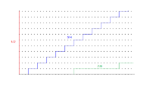
Figure 1: Payoff of the game on $h^{1}$,$h^{2}$ and $h^{3}$.

The uniform value exists in every state, is equal to $1$, and the decision maker has $\varepsilon$-optimal pure strategies: given an initial state, play $R$ until reaching some state in $h^{l}$ with $\frac{1}{2^{l}}\leq\varepsilon$ and then stay in $h^{l}$.

There exists no $0$-optimal pure strategy from state $(0,0)$. Since there is only one player, the transition is deterministic and the payoff depends only on the state, we can identify a pure strategy with the sequence of states it selects on the play that it defines. Let $h=(z_{1},...,z_{t},...)$ be a $0$-optimal strategy. Since the play $h$ guarantees $1$, there exists an increasing sequence of stages $(n_{l})_{l\geq 1}$ such that $h$ crosses $h^{l}$ at stage $n_{l}$.

Let $m_{l}<n_{l+1}$ be the last time before $n_{l+1}$ such that $h$ intersects $h^{l}$. The reader can check that then $n_{l+1}-m_{l}\geq m_{l}$, and every state of $h$ between stage $m_{l}+1$ and stage $n_{l+1}$ is in $h^{0}$. Therefore the expected average payoff at stage $n_{l+1}-1$ is less $\frac{1}{2}\times 1+\frac{1}{2}\times 0=\frac{1}{2}$.

We now argue that there is a behavioral strategy that yields payoff $1$. We start by illustrating a strategy that yields an expected average payoff at least $\frac{3}{8}$ in all stages:

• with probability $1/4$, the decision maker plays $3$ times Right in order to reach the set $h^{2}$ and then stays in $h^{2}$;

• with probability $1/4$, the decision maker stays in the set $h^{1}$ for $3$ stages ($3$ times Top) then plays $9$ times Right in order to reach the set $h^{2}$ and then stays in $h^{2}$;

• with probability $1/4$, the decision maker stays in the set $h^{1}$ for $3+9=12$ stages then plays $36$ times Right in order to reach the set $h^{2}$ and then stays in $h^{2}$;

• with probability $1/4$ the decision maker stays in the set $h^{1}$ for $3+9+36=48$ stages then plays $144$ times Right in order to reach the set $h^{2}$ and then stays in $h^{2}$.

Note that the state at stage $192$ is on $h^{2}$ and more precisely equal to $(48,144)$ whatever is the pure strategy chosen. The first strategy yields a payoff of $3/4$ except on the second and third times the decision maker is playing right (stage 2-3), the second one yields a payoff of $1/2$ before stage $3$ (included) and a payoff of $3/4$ from stages $13$ (included), the third one yields a payoff of $1/2$ before stage $12$ (included) and a payoff of $3/4$ from stage $49$ (included) and the fourth one yields a payoff of $1/2$ before stage $48$ (included) and a payoff of $3/4$ from stages $193$ (included).

Thus for each stage $n$ up to stage $192$, there is at most one of the four pure strategies that gives a daily payoff of $0$. The others strategies either stay in $h^{1}$ or stay in $h^{2}$, and thus yield a stage payoff at least $1/2$. Therefore, the expected payoff at each stage is greater than $\frac{3}{4}*\frac{1}{2}=\frac{3}{8}$ and the expected average payoff until stage $n$ is greater than $3/8$ for every $n\geq 1$. We managed to build a strategy going from $h^{1}$ to the set $h^{2}$ such that the expected average payoff does not drop below $\frac{3}{8}$.

We can iterate and switch from $h^{2}$ to $h^{3}$ without the payoff dropping below $\frac{7}{8}*\frac{3}{4}$ by considering $8$ different pure strategies. Repeating this procedure from $h^{l}$ to $h^{l+1}$ for every $l\geq 1$ will lead to a $0$-optimal strategy. To define properly a strategy which ensures an expected payoff $1$, we augment the strategy as in Section 4.3.

4.2 Existence of $\varepsilon$-optimal strategies with a constant value on the induced play

In this part, we consider a commutative deterministic MDP with a uniform value in pure strategies. We show that for all $x_{1}\in X$ and all $\varepsilon>0$ there exists an $\varepsilon$-optimal pure strategy in $\Gamma(x_{1})$ such that the value is constant on the induced play. Lehrer and Sorin [LS92] showed that in deterministic MDPs, given a sequence of actions, the value is always non-increasing along the induced play. In particular, it is true along the play induced by an $\varepsilon$-optimal pure strategy. We need to define an $\varepsilon$-optimal pure strategy such that the value is non-decreasing.

To this end, we introduce a partial preorder on the set of states such that, if $x^{\prime}$ is greater than $x$, then $x^{\prime}$ can be reached from $x$, i.e. there exists a finite sequence of actions such that $x^{\prime}$ is on one play induced from $x$. Fix a state $x_{1}$ and let $x$ be a state which can be reached from $x_{1}$. By commutativity, the order of actions is not relevant and we can represent the state $x$ by a vector $m\in\mathds{N}^{I}$, counting how many times each action has to be played in order to reach $x$ from $x_{1}$. Let $M(x)$ be the set of all vectors representing the state $x$.

Given two vectors $m$ and $m^{\prime}$ in $\mathds{R}^{I}$, $m$ is greater than $m^{\prime}$ if for every $i\in I$, $m(i)\geq m^{\prime}(i)$. Given two states $x$ and $x^{\prime}$, we say that $x$ is greater than $x^{\prime}$, denoted $x\geq x^{\prime}$, if there exists $m\in M(x)$ and $m^{\prime}\in M(x^{\prime})$, such that $m\geq m^{\prime}$. By construction, $x\geq x^{\prime}$ implies that $x$ can be reached from the state $x^{\prime}$. Indeed if $x$ is greater than $x^{\prime}$, then there exists $m\in M(x)$ and $m^{\prime}\in M(x^{\prime})$ such that $m\geq m^{\prime}$ in all coordinates. By playing $(m-m^{\prime})(i)$ times the action $i$ for every $i\in I$, the decision maker can reach the state $x$ from $x^{\prime}$.

Lemma 4.2

Consider a commutative deterministic MDP with a uniform value in pure strategies. For all $x_{1}\in X$ and all $\varepsilon>0$ there exists an $\varepsilon$-optimal strategy in $\Gamma(x_{1})$ such that the value is non-decreasing, thus constant, on the induced play.

Proof: Fix $x_{1}\in X$ and $\varepsilon>0$. We construct a sequence of real numbers $(\varepsilon_{l})_{l\geq 1}$ and a sequence of strategies $(\sigma^{l})_{l\geq 1}$ satisfying three properties. For each $l\geq 1$, we denote by $(x^{l}_{n})_{n\geq 1}$ the sequence of states along $\sigma^{l}$. First, the sequence $(\varepsilon_{l})_{l\geq 1}$ is decreasing and $\varepsilon_{1}\leq\varepsilon$ (property $(i)$). Second, for every $l\geq 1$ the strategy $\sigma^{l}$ is $\varepsilon_{l}$-optimal in the game $\Gamma(x_{1})$ (property $(ii)$). Finally, given any $l\geq 1$ and any stage $n\geq 1$, for every $l^{\prime}\geq l$ there exists a stage $n^{\prime}$ such that $x_{n^{\prime}}^{l^{\prime}}\geq x_{n}^{l}$ (property $(iii)$). This implies that $x_{n^{\prime}}^{l^{\prime}}$ is reachable from $x_{n}^{l}.$ Informally, a decision maker who follows the strategy $\sigma^{l}$ can change his mind in order to play better: at any stage he can stop following $\sigma^{l}$, choose any $l^{\prime}\geq l$, and play some actions such that the play merges eventually with the play induced by $\sigma^{l^{\prime}}$.

Let $(\varepsilon_{l})_{l\geq 1}$ be a decreasing sequence of positive numbers converging to $0$ such that $\varepsilon_{1}=\varepsilon$. For each $l\geq 1$, let $\sigma^{l}$ be an $\varepsilon_{l}$-optimal pure strategy in $\Gamma(x_{1})$. We identify $\sigma^{l}$ with the sequence of actions $(i_{1},i_{2},...)$ it induces. By construction, these sequences satisfy properties $(i)$ and $(ii)$. To satisfy property $(iii)$, we extract a subsequence.

For all $l\geq 1$ and all $n\geq 1$, considering the strategy $\sigma^{l}$ until stage $n$ defines a vector $m_{n}(\sigma^{l})$ in $M(x^{l}_{n})$. The sequence $(m_{n}(\sigma^{l}))_{n\geq 1}$ is non-decreasing in every coordinate, so we can define the limit vector $m_{\infty}(\sigma^{l})\in(\mathds{N}\times\{\infty\})^{I}$. By definition of the limit, for any $w\in\mathds{N}^{I}$ such that $w\leq m_{\infty}(\sigma^{l})$, there exists some stage $n$ such that $w\leq m_{n}(\sigma^{l})$.

Since the number of actions is finite, we can choose a subsequence of $(m_{\infty}(\sigma^{l}))_{l\geq 1}$ such that each coordinate is non-decreasing in $l$. Informally, the closer to the value the decision maker wants the payoff to be the more he has to play each action. We keep the same notation, and denote by $(\varepsilon_{l})_{l\geq 1}$ and $(\sigma^{l})_{l\geq 1}$ the sequences after extraction.

After extraction $\varepsilon_{1}$ is smaller than $\varepsilon$. By definition, $\sigma^{l}$ is $\varepsilon_{l}$-optimal in the game $\Gamma(x_{1})$. Moreover, given two integers $l,l^{\prime}$ such that $1\leq l\leq l^{\prime}$, we have $m_{\infty}(\sigma^{l})\leq m_{\infty}(\sigma^{l^{\prime}})$. Let $n$ be a positive integer, then

$$m_{n}(\sigma^{l})\leq m_{\infty}(\sigma^{l})\leq m_{\infty}(\sigma^{l^{\prime}}).$$

By definition of $m_{\infty}(\sigma^{l^{\prime}})$ as a limit, there exists a stage $n^{\prime}$ such that $m_{n^{\prime}}(\sigma^{l^{\prime}})$ is greater than $m_{n}(\sigma^{l})$, and thus $x^{l^{\prime}}_{n^{\prime}}$ is greater than $x^{l}_{n}$. The subsequences $(\varepsilon_{l})_{l\geq 1}$ and $(\sigma_{l})_{l\geq 1}$ satisfy all the properties $(i)-(iii)$.

We now deduce that the value along $\sigma_{1}$ is non decreasing: for every $n\geq 1$, the uniform value in state $x^{1}_{n}$ is equal to the uniform value in the initial state. Fix $n\geq 1$ and $l^{\prime}\geq 1$. By construction, there exists $n^{\prime}\geq n$ such that $x_{n^{\prime}}^{l^{\prime}}$ can be reached from state $x_{n}^{1}$. Applying Lehrer and Sorin [LS92], we know that the value is non increasing along plays so $v^{*}(x^{1}_{n})\geq v^{*}(x^{l^{\prime}}_{n^{\prime}}).$ Moreover, the strategy $\sigma^{l^{\prime}}$ defines a continuation strategy from $x^{l^{\prime}}_{n^{\prime}}$, which yields an average long-run payoff of at least $v^{*}(x_{1})-\varepsilon_{l^{\prime}}$. Thus, the uniform value along the play induced by $\sigma_{l^{\prime}}$ does not drop below $v^{*}(x_{1})-\varepsilon_{l^{\prime}}$:

$$v^{*}(x^{l^{\prime}}_{n^{\prime}})\geq v^{*}(x_{1})-\varepsilon_{l^{\prime}}.$$

Considering both results together, we obtain that

$$v^{*}(x^{1}_{n})\geq v^{*}(x^{l^{\prime}}_{n^{\prime}})\geq v^{*}(x_{1})-\varepsilon_{l^{\prime}}.$$

Since it is true for every $l^{\prime}\geq 1$, we deduce that the value is non decreasing along $\sigma_{1}$. In order to conclude, notice that $\varepsilon_{1}\leq\varepsilon$, therefore $\sigma_{1}$ is $\varepsilon$-optimal. $\Box$

4.3 Proof of Theorem 3.1(1)

In this subsection, we prove Theorem 3.1(1): in every commutative MDP with a uniform value in pure strategies, there exists a $0$-optimal strategy.

A strategy $\sigma$ is said to be partially $0$-optimal if the limsup of the sequence of expected average payoffs is equal to the uniform value: $\limsup_{n}\gamma_{n}(x_{1},\sigma)=v^{*}(x_{1})$. We first deduce from Lemma 4.2 the existence of partially $0$-optimal pure strategies. As shown in Example 4.1, expected average payoffs may not converge along partially $0$-optimal strategy and, in particular, can be small infinitely often. The key point of the proof of Theorem 3.1(1) is that different partially $0$-optimal strategies have bad expected average payoff at different stages. By choosing a proper mixed strategy that is supported by pure partially $0$-optimal strategies, we can ensure that, at each stage, the probability to play one pure strategy with a bad expected average payoff is small.

We will first provide the formal definition of partially $0$-optimal strategies and the concatenation of a sequence of strategies along a sequence of stopping times. Then, we define two specific sequences such that the concatenated strategy $\sigma^{*}$ is $0$-optimal. The proof of the optimality of $\sigma^{*}$ is done in two steps: we check that the support of $\sigma^{*}$ is included in the set of partially $0$-optimal strategies, and that the probability to play a strategy with a bad expected average payoff at stage $n$ converges to $0$ for $n$ sufficiently large.

We now start the proof of Theorem 3.1(1) by defining formally a partially $0$-optimal strategy.

Definition 4.3

Let $\Gamma=(X,I,q,g)$ be an MDP and $v^{*}(x_{1})$ be the uniform value of the MDP starting at $x_{1}$. A strategy $\sigma$ is partially $0$-optimal if

$$\limsup_{n}\gamma_{n}(x_{1},\sigma)=v^{*}(x_{1}).$$

That is, for every $\varepsilon>0$, the long run expected average payoff is greater than $v^{*}(x_{1})-\varepsilon$ infinitely often.

We define the concatenation of strategies with respect to a sequence of stopping times . Let $(u_{l})_{l\geq 2}$ be a sequence of increasing stopping times and $(\sigma_{l})_{l\geq 1}$ be a sequence of strategies. The concatenated strategy $\sigma^{*}$ is defined as follows. For every $t\geq 1$ and every $h_{t}=(x_{1},i_{1},j_{1},...,x_{t})$, let $l^{*}=l^{*}(h_{t})=\sup\{l,u_{l}(h_{t})\leq t\}$ and $\sigma^{*}(h_{t})=\sigma_{l^{*}}(h^{u_{l}^{*}}_{t})$ where $h^{u_{l}^{*}}_{t}=(x_{u_{l}^{*}},i_{u_{l}^{*}},j_{u_{l}^{*}}...,x_{t})$. Informally, for every $l\geq 2$, at stage $u_{l}$ the decision maker forgets the past history and follows $\sigma_{l}$.

Definition of the $0$-optimal strategy: Fix $x_{1}\in X$. For every $t\geq 1$, we denote by $X(t)$ the set of states which can be reached from $x_{1}$ in less than $t$ stages. Since the transition is deterministic and the number of actions is finite, the set $X(t)$ is finite for every $t\geq 1$. We choose two specific sequences of stopping times and strategies and denote by $\sigma^{*}$ the concatenation. Let $(\varepsilon_{l})_{l\geq 1}$ be a decreasing sequence of real numbers converging to $0$. For each $x\in X$ and every integer $l\geq 1$, we denote by $\sigma_{l}(x)$ an $\varepsilon_{l}$-optimal strategy in $\Gamma(x)$ such that the uniform value is constant on the play, and let $N(l,x)$ be an integer that satisfies

$$\forall n\geq N(l,x),\ \gamma_{n}(x,\sigma_{l}(x))\geq v^{*}(x)-\varepsilon_{l}.$$ (1)

In any games longer than $N(l,x)$ stages, the average expected payoff is close to the value, but the payoff in shorter games is not controlled. The strategy $\sigma_{l}(x)$ exists by Lemma 4.2.

We now define the sequence of stopping times. For every $l\geq 1$, we define a set of stages $T_{l}$ and let $u_{l}$ be a stopping time uniformly distributed over $T_{l}$. Start by setting $t_{1}=1$ and $T_{1}=\{1\}$. Let $l\geq 1$ and assume that the set $T_{l}$ is already defined. Denote $t_{l+1}=\left[\frac{1}{\varepsilon_{l+1}}\right]+1$ and define the set $T_{l+1}=\{T_{l+1}^{(1)},...,T_{l+1}^{(t_{l+1})}\}$ by induction:

$$T_{l+1}^{(1)} =T_{l}^{(t_{l})}+\max_{x\in X(T_{l}^{(t_{l})})}N(l,x)+\left[\frac{1}{\varepsilon_{l}}+1\right]T_{l}^{(t_{l})},$$

$$T_{l+1}^{(2)} =T_{l+1}^{(1)}+\max_{x\in X({T_{l+1}^{(1)}})}N(l+1,x),$$

$$... ,...$$

$$T_{l+1}^{(t_{l+1})} =T_{l+1}^{(t_{l+1}-1)}+\max_{x\in X(T_{l+1}^{(t_{l+1}-1)})}N\left(l+1,x\right).$$

Let $t\in T_{l+1}$, we call the smallest integer strictly greater than $t$ in $T_{l+1}\cup T_{l+2}$, the successor of $t$. Formally, there exists $c_{l+1}\leq t_{l+1}$ such that $t=T_{l+1}^{(c_{l+1})}$. If $c_{l+1}$ is strictly smaller than $t_{l+1}$, the successor of $t$ is $T_{l+1}^{(c_{l+1}+1)}$; if $c_{l+1}=t_{l+1}$, then the successor of $t$ is $T_{l+2}^{(1)}$.

We make few comments on the definition of the set $T_{l+1}$. First, the number of stages between two different integers $t$ and $t^{\prime}$ in $T_{l+1}$ is such that a strategy, which starts playing like $\sigma_{l+1}(x_{t})$ at stage $t$ yields an expected average payoff between stage $t$ and stage $t^{\prime}-1$ greater than $v^{*}(x_{1})-\varepsilon_{l+1}$. Second, the weight of the first $T_{l}^{t_{l}}$ stages in a game of length $T_{l+1}^{1}$ is small.

We prove that the strategy $\sigma^{*}(x_{1})$ is $0$-optimal. We consider here $\sigma^{*}(x_{1})$ as a mixed strategy, i.e. a probability over pure strategies. More precisely, let $\Omega$ be the set of pure strategies defined as concatenation of a sequence of integers $(n_{l})_{l\geq 2}$ with $n_{l}\in T_{l}$ for every $l\geq 2$ and the sequence of strategy $(\sigma_{l})_{l\geq 1}$. $\sigma^{*}$ is a probability over $\Omega$.

We show that every pure strategy in $\Omega$ is partially $0$-optimal.

Lemma 4.4

Let $(n_{l})_{l\geq 2}$ be a sequence of integers such that for every $l\geq 2$, $n_{l}\in T_{l}$. Denote by $\sigma$ the concatenated strategy induced by $(n_{l})_{l\geq 2}$ and $(\sigma_{l})_{l\geq 1}$.

The strategy $\sigma$ is partially $0$-optimal. Moreover, we have explicit lower bounds for specific stages. For every $l\geq 2$, let $n^{\prime}_{l}$ be the successor of $n_{l}$. Then

$$\forall l\geq 2,\ \forall n\in[n^{\prime}_{l}-1,n_{l+1}-1],\ \gamma_{n}(x_{1},\sigma)\geq v^{*}(x_{1})-2\varepsilon_{l-1}.$$

Proof: We first show that the sequence $\gamma_{n_{l+1}-1}(x_{1},\sigma)$ converges to the uniform value $v^{*}(x_{1})$ when $l$ goes to $\infty.$ At stage $n_{l}$, the strategy $\sigma$ starts to follow an $\varepsilon_{l}$-optimal strategy from the current state. By definition, $n^{\prime}_{l}-n_{l}\geq N(l,x_{n_{l}})$, and thus by Equation (1)

$$\gamma_{n_{l},n^{\prime}_{l}-1}(x_{1},\sigma)=\gamma_{n^{\prime}_{l}-n_{l}}(x_{n_{l}},\sigma_{l}(x_{n_{l}}))\geq v^{*}(x_{n_{l}})-\varepsilon_{l}\geq v^{*}(x_{1})-\varepsilon_{l}.$$

More generally, for every $n\in[n^{\prime}_{l}-1,n_{l+1}-1]$, we have

$$\gamma_{n_{l},n}(x_{1},\sigma)=\gamma_{n-n_{l}+1}(x_{n_{l}},\sigma_{l}(x_{n_{l}}))\geq v^{*}(x_{1})-\varepsilon_{l}.$$

In particular we have

$$\gamma_{n_{l},n_{l+1}-1}(x_{1},\sigma) \geq v^{*}(x_{1})-\varepsilon_{l}.$$ (2)

The expected average payoff between stage $n_{l}$ and $n_{l+1}-1$ is greater than $v^{*}(x_{1})-\varepsilon_{l}.$ It follows that the sequence $(\gamma_{n_{l+1}-1}(x_{1},\sigma))_{l\geq 1}$ converges to $v^{*}(x_{1})$ and therefore the strategy $\sigma$ is partially $0$-optimal.

We now prove the second part of the lemma, giving some explicit subsequences and bounds on the rate of convergence: for all $l\geq 2$, for all $n$ between $n^{\prime}_{l}-1$ and $n_{l+1}-1$, we prove that

$$\gamma_{n}(x_{1},\sigma)\geq v^{*}(x_{1})-2\varepsilon_{l-1}.$$ (3)

Fix $l\geq 2$. We first prove this lower bound for the expected average payoff until stage $n_{l}-1$ (which is before $n^{\prime}_{l}-1$). By definition of $T_{l}^{1}$, the weight of the $n_{l-1}$ first stages is small in the MDP of length $n_{l}-1$:

$$\frac{n_{l-1}-1}{n_{l}-1}\leq\frac{n_{l-1}-1}{T_{l}^{(1)}-1}\leq \frac{T_{l-1}^{(t_{l-1})}}{T_{l-1}^{(t_{l-1})}+N(l-1,x_{T_{l-1}^{(t_{l-1})}})-1+\left[\frac{1}{\varepsilon_{l-1}}+1\right]T_{l-1}^{(t_{l-1})}}$$

$$\leq\frac{T_{l-1}^{(t_{l-1})}}{\left[\frac{1}{\varepsilon_{l-1}}+1\right]T_{l-1}^{(t_{l-1})}}\leq\varepsilon_{l-1}.$$

Using Equation (2) for $l^{\prime}=l-1$ and the previous equation, it follows that

$$\gamma_{n_{l}-1}(x_{1},\sigma) =\left[\frac{n_{l-1}-1}{n_{l}-1}\gamma_{n_{l-1}-1}(x_{1},\sigma)+\frac{n_{l}-n_{l-1}}{n_{l}-1}\gamma_{n_{l-1},n_{l}-1}(x_{1},\sigma)\right],$$

$$\geq\left[\gamma_{n_{l-1},n_{l}-1}(x_{1},\sigma)-\frac{n_{l-1}-1}{n_{l}-1}\right],$$

$$\geq v^{*}(x_{1})-2\varepsilon_{l-1}.$$

Let $n$ be a positive integer between $n^{\prime}_{l}-1$ and $n_{l+1}-1$. The expected average payoff until stage $n$ is the convex combination of the expected average payoff until stage $n_{l}-1$ (before $n^{\prime}_{l}-1$) and the average expected payoff between stages $n_{l}$ and $n$. Both of these quantities are greater than $v^{*}(x_{1})-2\varepsilon_{l-1}$, and therefore their convex combination is greater than $v^{*}(x_{1})-2\varepsilon_{l-1}$ as well. $\Box$

Remark 4.5

Following the notation of Lemma 4.4, if $n\in\cup_{l\geq 2}[n_{l},n^{\prime}_{l}-2]$ then we only know that the $n$-stage expected average payoff is greater than $0$.

Lemma 4.6

$\sigma^{*}(x_{1})$ is a $0$-optimal strategy.

Proof: We consider here $\sigma^{*}(x_{1})$ as a mixed strategy. Lemma 4.4 showed that with probability one the pure strategies in the support of $\sigma^{*}$ are partially $0$-optimal.

Let $l\geq 2$ and fix $n$ an integer in $[T^{1}_{l},T^{1}_{l+1}-1]$. We show that, with probability higher than $1-\varepsilon_{l}$, the decision maker is following a pure strategy giving an expected average payoff until stage $n$ higher than $v^{*}(x_{1})-2\varepsilon_{l-2}$.

By definition, there exists a unique stage $n^{*}_{l}$ in $T_{l}$ such that $n$ is between $n^{*}_{l}$ and $n^{\prime*}_{l}-1$ where $n^{\prime*}_{l}$ is the successor of $n^{*}_{l}$:

$$n_{l}^{*}\leq n\leq n^{\prime*}_{l}-1.$$ (4)

Let $\sigma$ be a pure strategy with positive probability under $\sigma^{*}$. There exists a sequence $(n_{d})_{d\geq 2}$ such that for all $d\geq 2$, $n_{d}\in T_{d}$ and $\sigma$ is the concatenated strategy induced by $(n_{d})_{d\geq 2}$ and $(\sigma_{d})_{d\geq 1}$. We follow the previous notation and denote for every $d\geq 2$, the successor of $n_{d}$ by $n^{\prime}_{d}$. Since $n\in[T^{1}_{l},T^{1}_{l+1}-1]$, by construction of the sets $T_{l-1}$,$T_{l}$, and $T_{l+1}$, we have

$$n^{\prime}_{l-1}\leq n\leq n_{l+1}-1.$$ (5)

We now use the inequalities (4) and (5) to handle the three different cases depending on the respective places of $n^{*}_{l}$, the beginning of the block containing $n$, and $n_{l}$, the stage where the strategy $\sigma$ is switching from an $\varepsilon_{l-1}$ strategy to an $\varepsilon_{l}$-optimal strategy: $n_{l}>n^{*}_{l}$, $n_{l}<n^{*}_{l}$, and $n_{l}=n^{*}_{l}$.

If $n_{l}>n^{*}_{l}$, then at stage $n$ the pure strategy $\sigma$ is still following the $\varepsilon_{l-1}$-optimal strategy from state $x_{n_{l-1}}$ and therefore yields a high expected average payoff. Formally, we have $n^{\prime}_{l-1}\leq n\leq n^{\prime*}_{l}-1\leq n_{l}-1$, so that by Lemma 4.4 applied to $l^{\prime}=l-1$,

$$\gamma_{n}(x_{1},\sigma)\geq v^{*}(x_{1})-2\varepsilon_{l-2}.$$

If $n_{l}<n^{*}_{l}$, then at stage $n$, the pure strategy $\sigma$ has already followed the $\varepsilon_{l}$-optimal strategy from state $x_{n_{l}}$ for a long time and thus yields a high expected average payoff. Formally, we have $n^{\prime}_{l}\leq n^{*}_{l}\leq n\leq n_{l+1}-1$, so that by Lemma 4.4 applied to $l$,

$$\gamma_{n}(x_{1},\sigma)\geq v^{*}(x_{1})-2\varepsilon_{l-1}\geq v^{*}(x_{1})-2\varepsilon_{l-2}.$$

Finally if $n_{l}=n^{*}_{l}$, we do not control the expected average payoff but by definition of the stopping time $u_{l}$ the probability of the event $\{n_{l}=n^{*}_{l}\}$ is smaller than $\varepsilon_{l}$ under $\sigma^{*}$.

We can now conclude. We denote by $\mathds{P}_{\sigma^{*}}$ the probability distribution induced by $\sigma^{*}$ on the set of pure strategy and $\mathds{E}_{\sigma^{*}}$ the corresponding expectation. Since the payoffs are in $[0,1]$, it follows that

$$\gamma_{n}(x_{1},\sigma^{*})=\mathds{E}_{\sigma^{*}}\left(\gamma_{n}(x_{1},\sigma)\right)\geq(1-\varepsilon_{l})(v^{*}(x_{1})-2\varepsilon_{l-2})\geq v^{*}(x_{1})-3\varepsilon_{l-2}.$$

This is true for every $l\geq 1$ and every integer $n\in[T^{1}_{l},T^{1}_{l+1}-1]$, therefore the expected average payoff converges to the uniform value: the strategy $\sigma^{*}$ is $0$-optimal.$\hfill\Box$

4.4 Proof of Theorem 3.1(2)

In this section, we prove Theorem 3.1(2): namely, if the set of states $X$ is a precompact metric space, the transition is $1$-Lipschitz, deterministic, and commutative, and the payoff function is uniformly continuous, then there exists a pure $0$-optimal strategy.

We will first justify the existence of the uniform value and that we can assume that the set of states is compact. Then, we will define recursively a sequence of states $(x^{l})_{l\geq 1}$ such that $x^{1}=x_{1}$ and $x^{l+1}$ is a limit point of states along an $\varepsilon_{l}$-optimal pure strategy $\sigma^{l}(x^{l})$ starting from $x^{l}$ where the value is constant on the induced play. Therefore, the value in all these states is equal to $v^{*}(x_{1})$.

For each $l\geq 1$ we will define by induction a sequence of stages $(n^{l}_{k})_{k\geq 1}$ such that the sequence of states induced by $\sigma^{l}$ at stages $n^{l}_{k}$ converges to the limit point $x^{l+1}$. We impose in addition conditions on $n^{l}_{l+1}$ and on the speed of convergence. This sequence of stages splits the strategy $\sigma^{l}$ into a finite sequence of streaks of actions. Given $k\geq 1$, we call an elementary block the streak of actions played between stage $n^{l}_{k-1}$ and $n^{l}_{k}$. Note that it has $n^{l}_{k}-n^{l}_{k-1}$ actions. By convention, the first block starts at stage $n^{l}_{0}=1$.

We will define the $0$-optimal strategy $\sigma^{*}$ by playing these elementary blocks in a specific order. The strategy $\sigma^{*}$ is defined as a succession of two types of blocks $(A_{l})_{l\geq 1}$ and $(B_{l})_{l\geq 1}$ such that for all $l\geq 1$, $A_{l}$ is composed of $l+1$ consecutive elementary blocks from $\sigma^{l}(x^{l})$ and $B_{l}$ is composed of $l-1$ elementary blocks, one from each $\sigma^{l^{\prime}}(x^{l^{\prime}})$ for $1\leq l^{\prime}\leq l-1$:

$$\sigma^{*}=(A_{1},B_{1},A_{2},B_{2},A_{3},....).$$

Block $B_{l-1}$ ensures that the distance between the state at the beginning of block $A_{l}$ and $x^{l}$ is small. Block $A_{l}$ guarantees an expected average payoff close to the value up to a function of $\varepsilon_{l}$. Moreover, block $A_{l}$ is long enough for the total expected average payoff of $\sigma^{*}$ at the end of $A_{l}$ to be close to the value. It will follow that the strategy $\sigma^{*}$ is partially $0$-optimal. The rest of the proof consists in showing that the expected average payoff does not drop between these stages, neither during block $B_{l+1}$ nor during the first stages of $A_{l+1}$. It follows that the strategy is $0$-optimal.

Let $\Gamma=(X,I,J,q,g)$ be a deterministic commutative MDP with a precompact metric space, a uniformly continuous payoff function and a $1$-Lipschitz transition. We first justify the existence of the uniform value. We follow Section 6.1 in Renault [Ren11]. Let $\Psi=(Z,F,r)$ be an auxilliary dynamic programming problem. The set of states is $Z=X\times I$, the correspondence is given by

$$\forall(x,i)\in Z,\ F(x,i)=\{(q(x,a),a),\ a\in I\},$$

and the payoff function is for all $(x,i)\in Z$, $r(x,i)=g(x,i).$ We consider on $Z$ the following metric $D((x,i),(x^{\prime},i^{\prime})=\max(d(x,x^{\prime}),\delta_{i\neq i^{\prime}}).$ The set of states $(Z,D)$ is precompact metric, the correspondence is $1$-Lipschtiz (i.e. for all $z,z^{\prime}\in Z,z_{1}\in F(z)$ there exists $z^{\prime}_{1}\in F(z)$ such that $D(z_{1},z^{\prime}_{1})\leq D(z,z^{\prime})$ ) and the payoff function is equicontinuous. By Corollary 3.9 of the same paper [Ren11], $\Psi$ has a uniform value for any initial state. We can deduce immediatly that $\Gamma(x_{1})$ has a uniform value for every $x_{1}\in X$.

We now prove that we can assume that $X$ is compact. Define an MDP $\hat{\Gamma}(\hat{X},I,\hat{q},\hat{g})$ as follows: $\hat{X}$ is the Cauchy completion of $X$, $\hat{q}$ is the $1$-Lipschitz extension of $q$ to $\hat{X}$, $\hat{g}$ is the uniformly continuous extension of $g$ to $\hat{X}$. By Renault [Ren11] and previous paragraph, both MDPs $\Gamma$ and $\hat{\Gamma}$ have a uniform value for any initial state.

Moreover the previous construction defines the transition on new states but does not change its value whenever it was already defined: for any state $x_{1}$ in $X$, $\hat{q}$ and $q$ coincides, as well as $g$ and $\hat{g}$. Therefore the MDPs $\Gamma(x_{1})$ and $\hat{\Gamma}(x_{1})$ are the same MDP on $X$. It follows that they have the same value.

In the following we assume that $X$ is compact. Let $x_{1}\in X$ and let $(\varepsilon_{l})_{l\geq 1}$ be a decreasing sequence of positive real numbers that converges to $0$. For each $x\in X$ and $l\geq 1$ denote by $\sigma_{l}(x)$ an $\varepsilon_{l}$-optimal pure strategy in $\Gamma(x)$ such that the value along the induced play is constant, and by $N(l,x)$ an integer such that

$$\forall n\geq N(l,x),\ \gamma_{n}(x,\sigma_{l}(x))\geq v^{*}(x)-\varepsilon_{l}.$$

Since $g$ is uniformly continuous, there exists $(\eta_{l})_{l\geq 1}$ such that

$$\forall x,x^{\prime}\in X,\ d(x,x^{\prime})\leq\eta_{l},\ \forall a\in\Delta(I),\ |g(x,a)-g(x^{\prime},a)|\leq\varepsilon_{l}.$$

Let $\sigma=(i_{t})_{t\geq 1}\in I^{\infty}$ be an infinite sequence of actions and let $x_{1}$ and $x_{1}^{\prime}$ be two initial states. For every $n\geq 1$, the distance between $x_{n}$, the state at stage $n$ obtained along the play induced by $x_{1}$ and $\sigma$, and $x^{\prime}_{n}$, the state at stage $n$ obtained along the play induced by $x^{\prime}_{1}$ and $\sigma$, is smaller than $d(x_{1},x^{\prime}_{1})$. It follows that

$$\forall x_{1},x^{\prime}_{1}\in X,\ s.t.\ d(x_{1},x^{\prime}_{1})\leq\eta_{l},\ \forall\sigma=(i_{t})_{t\geq 1}\in I^{\infty},\ \forall n\geq 1,\ |\gamma_{n}(x_{1},\sigma)-\gamma_{n}(x^{\prime}_{1},\sigma)|\leq\varepsilon_{l}.$$

Definition of the strategy $\sigma^{*}$: Let $x^{1}=x_{1}$. Given $(x^{j})_{1\leq j\leq l}$ define $x^{l+1}$ to be a limit point of the play $(x^{l},\sigma_{l}(x^{l}))$. Since the value is constant on the play induced by $(x^{l},\sigma_{l}(x^{l}))$, the uniform value in $x^{l+1}$ is also equal to $v^{*}(x_{1})$. To construct the $0$-optimal strategy, we split each play $\sigma_{j}(x^{j})$ into blocks by induction on $j$.

Let us assume that $(n^{j}_{k})_{k\geq 1}$ have been defined for every $j\leq l-1$, i.e. the splittings of all strategies $\{\sigma_{1}(x^{1}),...,\sigma_{l-1}(x^{l-1}\}$ have been defined. We now split the sequence $\sigma_{l}(x^{l})$.

Define $L_{l}=1+\sum_{j\leq{l-1}}(n^{j}_{l}-1)$, which depends only on the sequences for $j\leq(l-1)$. We denote by $(x^{l}_{n})_{n\geq 1}$ the sequence of states along $(x^{l},\sigma_{l}(x^{l}))$. Let us define the sequence of stages $(n^{l}_{k})_{k\geq 1}$ such that it satisfies four properties. The three first properties are restriction on $n^{l}_{l+1}$ and the last one is a restriction on the rate of convergence to $x^{l+1}$. First the strategy $\sigma_{l}(x^{l})$ guarantees in $\Gamma(x^{l})$ the value with an error less than $\varepsilon_{l}$ in all games longer than $n^{l}_{l+1}$:

$$n^{l}_{l+1} \geq N(l,x^{l}).$$ (6)

Second, $L_{l}$ is small compared to $n^{l}_{l+1}$:

$$\frac{L_{l}}{n^{l}_{l+1}}\leq\varepsilon_{l}.$$ (7)

Third,

$$\frac{N(l+1,x^{l+1})+\sum_{j=1}^{l-1}{\left(n^{j}_{l+1}-n^{j}_{l}\right)}}{n^{l}_{l+1}}\leq\varepsilon_{l}.$$ (8)

Finally, at the beginning of the $k$-th block of this decomposition the state is close to the limit point

$$d(x^{l}_{n^{l}_{k}},x^{l+1})\leq\frac{\eta_{k}}{k-1}.$$ (9)

Fix $l\geq 1$. We define $A_{l}$ to be the finite sequence of actions given by $\sigma^{l}(x^{l})$ between stage $1$ and stage $n^{l}_{l+1}$. In term of elementary blocks, it is composed of the first $l+1$ elementary blocks of $\sigma^{l}(x^{l})$ and is composed of $n^{l}_{l+1}-1$ actions. We define $B_{l}$ as the sequence of actions where the decision maker is playing, for each $l^{\prime}<l$, the elementary block of $\sigma^{l^{\prime}}(x^{l^{\prime}})$ between stages $n^{l^{\prime}}_{l}$ and $n^{l^{\prime}}_{l+1}$. Thus $B_{l}$ is the concatenation of $l-1$ elementary blocks. Moreover the number of actions in $B_{l}$ is $b_{l}=\sum_{j=1}^{l-1}{\left(n^{j}_{l+1}-n^{j}_{l}\right)}$, which appeared in (8). The strategy $\sigma^{*}$ is the sequence of actions given by the alternating sequence $(A_{l},B_{l})_{l\geq 1}$.

We now show that the strategy $\sigma^{*}$ is $0$-optimal.

We first prove that the state at the beginning of $A_{l}$ is close to $x^{l}$. Therefore the expected average payoff of $\sigma^{*}$ at the end of $A_{l}$ is bigger than $v^{*}(x_{1})-3\varepsilon_{l}$ and $\sigma^{*}$ is partially $0$-optimal.

Lemma 4.7

The payoff at the end of $A_{l}$ is greater than $v^{*}(x_{1})-3\varepsilon_{l}$:

$$\gamma_{L_{l}+n^{l}_{l+1}-1}(x_{1},\sigma^{*})\geq v^{*}(x_{1})-3\varepsilon_{l}$$

Corollary 4.8

The strategy $\sigma^{*}$ is partially $0$-optimal.

Proof of Lemma 4.7: Let us denote by $(x_{n})_{n\geq 1}$ the sequence of states on the play induced by $\sigma^{*}$.

We first prove that the state at the beginning of $A_{l}$ is close to $x^{l}$. One can verify that the first stage of $A_{l}$ is the stage $L_{l}=1+\sum_{j\leq{l-1}}(n^{j}_{l}-1)$. By definition, at stage $L_{l}$ for each $l^{\prime}\leq l-1$, all first $l$ elementary blocks of $\sigma^{l^{\prime}}(x^{l^{\prime}})$ have been played: all of the first $l^{\prime}+1$ on block $A_{l^{\prime}}$ and then one after each other in the blocks $B_{j}$ for $j\in[l^{\prime}+1,l-1]$. By commutativity, the state does not depend on the order of actions and the state is the same as after the sequence $\sigma^{\prime}$ where the decision maker plays $\sigma_{1}(x^{1})$ for $n^{1}_{l}-1$ stages, $\sigma_{2}(x^{2})$ for $n^{2}_{l}-1$ stages,…, and $\sigma_{l-1}(x^{l-1})$ for $n^{l-1}_{l}-1$ stages.

For each strategy $\sigma_{j}$, Equation (9) implies that the distance between $x^{j+1}$ and the state at stage $n^{j}_{l}$ on the play from $x^{j}$ is less than $\frac{\eta_{l}}{l-1}$ for each $j\in\{1,...,l-1\}$. The map $q$ is $1$-Lipschitz, so the distances sum up and an immediate induction implies that

$$d(x_{L_{l}},x^{l})\leq\eta_{l}.$$ (10)

Let us now compute the payoff in the MDP of length $L_{l}+n^{l}_{l+1}-1$, i.e. until the end of $A_{l}$. Equation (7) ensures that the payoff is almost equal to the payoff between stages $L_{l}$ and $L_{l}+n^{l}_{l+1}-1$:

$$\gamma_{L_{l}+n^{l}_{l+1}-1}(x_{1},\sigma^{*}) =\frac{L_{l}-1}{L_{l}+n^{l}_{l+1}-1}\gamma_{L_{l}-1}(x_{1},\sigma^{*})+\frac{n^{l}_{l+1}}{L_{l}+n^{l}_{l+1}-1}\gamma_{L_{l},L_{l}+n^{l}_{l+1}-1}(x_{1},\sigma^{*})$$

$$\geq\frac{n^{l}_{l+1}}{L_{l}+n^{l}_{l+1}-1}\gamma_{L_{l},L_{l}+n^{l}_{l+1}-1}(x_{1},\sigma^{*})$$

$$\geq\gamma_{L_{l},L_{l}+n^{l}_{l+1}-1}(x_{1},\sigma^{*})-\frac{L_{l}-1}{L_{l}+n^{l}_{l+1}-1}$$

$$\geq\gamma_{L_{l},L_{l}+n^{l}_{l+1}-1}(x_{1},\sigma^{*})-\varepsilon_{l}.$$

Moreover $\sigma^{*}$ plays like an $\varepsilon_{l}$-optimal strategy in $\Gamma(x^{l})$ between stages $L_{l}$ and $L_{l}+n^{l}_{l+1}-1$, and the distance between $x_{L_{l}}$ and $x^{l}$ is less than $\eta_{l}$ by Equation (10). Therefore, by Equation (6) we have

$$\gamma_{L_{l}+n^{l}_{l+1}-1}(x_{1},\sigma^{*}) \geq\gamma_{n^{l}_{l+1}}(x_{L_{l}},\sigma_{l}(x^{l}))-\varepsilon_{l}$$

$$\geq\gamma_{n^{l}_{l+1}}(x^{l},\sigma_{l}(x^{l}))-2\varepsilon_{l}$$

$$\geq v^{*}(x_{1})-3\varepsilon_{l}.$$

$\hfill\Box$

We now check that the average expected payoff does not drop between these stages. We distinguish between two different cases: if $n\in[L_{l}+n^{l}_{l+1}-1,L_{l+1}+N(l+1,x^{l+1})]$ or if $n\in[L_{l+1}+N(l+1,x^{l+1}),L_{l+1}+n^{l+1}_{l+2}-1]$.

In the first case, the MDP ends at a stage in $B_{l}$ or in the beginning of block $A_{l+1}$. Equation (8) implies that the length of the game is almost equal to $L_{l}+n^{l}_{l+1}-1$, therefore the expected average payoff is greater than $v^{*}(x_{1})-4\varepsilon_{l}$.

In the second case, the MDP ends in the middle of block $A_{l+1}$. The expected average payoff is the convex combination of the expected average payoff until $L_{l+1}-1$ and the average expected payoff between $L_{l+1}$ and $n$. We check that both of them are high and we deduce that the expected average payoff is greater than $v^{*}(x_{1})-4\varepsilon_{l}$.

Lemma 4.9

Let $n\in[L_{l}+n^{l}_{l+1}-1,L_{l+1}+N(l+1,x^{l+1})]$. Then

$$\gamma_{n}(x_{1},\sigma^{*})\geq v^{*}(x_{1})-4\varepsilon_{l}.$$

The expected average payoff in any $n$-stage MDP such that $n$ is in the middle of block $B_{l}$ or at the beginning of block $A_{l+1}$ is greater than $v^{*}(x_{1})-4\varepsilon_{l}.$

Proof: The key point is that the number of stages is close to the case of Lemma 4.7. Let $n\in[L_{l}+n^{l}_{l+1}-1,L_{l+1}+N(l+1,x^{l+1})]$. By equation (8), we have

$$n-L_{l}-n^{l}_{l+1}+1 \leq N(l+1,x^{l+1})+\sum_{j=1}^{l-1}{(n^{j}_{l+1}-n^{j}_{l})}$$

$$\leq\varepsilon_{l}n_{l+1}^{l}.$$

It follows that

$$\gamma_{n}(x_{1},\sigma^{*}) =\frac{L_{l}+n^{l}_{l+1}-1}{n}\gamma_{L_{l}+n^{l}_{l+1}-1}(x_{1},\sigma^{*})+\frac{n-L_{l}-n^{l}_{l+1}+1}{n}\gamma_{L_{l}+n^{l}_{l+1},n}(x_{1},\sigma^{*})$$

$$\geq\frac{L_{l}+n^{l}_{l+1}-1}{n}\gamma_{L_{l}+n^{l}_{l+1}-1}(x_{1},\sigma^{*})$$

$$\geq\gamma_{L_{l}+n^{l}_{l+1}-1}(x_{1},\sigma^{*})-\frac{n-L_{l}-n^{l}_{l+1}+1}{n}$$

$$\geq v^{*}(x_{1})-3\varepsilon_{l}-\frac{n-L_{l}-n^{l}_{l+1}+1}{n^{l}_{l+1}}$$

$$\geq v^{*}(x_{1})-4\varepsilon_{l}.\hfill\Box$$

Lemma 4.10

Let $n\in[L_{l+1}+N(l+1,x^{l+1}),L_{l+1}+n^{l+1}_{l+2}-1]$. Then

$$\gamma_{n}(x_{1},\sigma^{*})\geq v^{*}(x_{1})-4\varepsilon_{l}.$$

The payoff in any $n$-stage MDP stopping in the middle of block $A_{l+1}$ is greater than $v^{*}(x_{1})-4\varepsilon_{l}.$

Proof: Let $n\in[L_{l+1}+N(l+1,x^{l+1}),L_{l+1}+n^{l+1}_{l+2}-1]$. The expected average payoff is the convex combination of the expected average payoff until $L_{l}+n^{l}_{l+1}-1$ and the expected average payoff between $L_{l}+n^{l}_{l+1}-1$ and $n$. It follows that

$$\gamma_{n}(x_{1},\sigma^{*}) =\frac{L_{l+1}-1}{n}\gamma_{L_{l+1}-1}(x_{1},\sigma^{*})+\frac{n-(L_{l+1}-1)}{n}\gamma_{L_{l+1},n}(x_{1},\sigma^{*})$$

$$=\frac{L_{l+1}-1}{n}\gamma_{L_{l+1}-1}(x_{1},\sigma^{*})+\frac{n-(L_{l+1}-1)}{n}\gamma_{n-L_{l+1}+1}(x_{L_{l+1}},\sigma_{l+1}(x_{L_{l+1}}))$$

$$\geq\frac{L_{l+1}-1}{n}(v^{*}(x_{1})-4\varepsilon_{l})+\frac{n-(L_{l+1}-1)}{n}(v^{*}(x^{l+1})-2\varepsilon_{l+1})$$

$$\geq v^{*}(x_{1})-4\varepsilon_{l}.$$

The expected average payoff is greater than $v^{*}(x_{1})-4\varepsilon_{l}$. $\Box$

Lemma 4.9 and Lemma 4.10 are true for every $l\geq 1$, therefore the strategy $\sigma^{*}$ is pure and $0$-optimal at $x_{1}$, which concludes the proof.

5 Commutative stochastic games.

In this section, we focus on commutative stochastic games and state-blind repeated games. In Section 5.1, we show that the class of absorbing games is in fact a subclass of commutative stochastic games. We show that each absorbing state can be replaced by a non-absorbing state leading to some new states, which are useless from a strategic point of view but designed in order to fulfill the commutativity assumption. In Section 5.2, we prove the existence of the uniform value in stochastic games with a deterministic commutative $1$-Lipschitz transition (Theorem 3.6). In Section 5.3, we deduce the existence of the uniform value in state blind commutative repeated games (Corollary 3.7). In Section 5.4, we provide some generalizations.

5.1 Absorbing games

Absorbing games were introduced by Kohlberg [Koh74]. They are stochastic games with a single non-absorbing state. An absorbing game is thus given by $\Gamma=(\{\alpha\}\cup X,I,J,q,g)$ where $\alpha$ is the unique non-absorbing state and all states $x\in X$ are absorbing: $q(x,i,j)(x)=1\ \forall x\in X,i\in I,j\in J.$ The state $\alpha$ is the only state where the players have an influence on the payoff and on future states. For each action pair $(i,j)\in I\times J$, we denote by $q(\alpha,i,j)(X)$ the total probability to reach an absorbing state by playing the action pair $(i,j)$.

Proposition 5.1

Let $\Gamma=(\{\alpha\}\cup X,I,J,q,g)$ be an absorbing game. There exists a commutative game $\Gamma^{\prime}=(X^{\prime},I,J,q^{\prime},g^{\prime})$ and a state $\alpha_{2}^{\prime}\in X^{\prime}$ such that for all $n\geq 1$, $v_{n}(\alpha)=v^{\prime}_{n}(\alpha_{2}^{\prime}).$ Moreover a player can guarantee $w$ in $\Gamma^{\prime}(\alpha_{2}^{\prime})$ if and only if he can guarantee $w$ in $\Gamma(\alpha)$.

Proof: Let $q(\alpha,i,j|X)$ be the conditional probability on $X$ if the action pair $(i,j)$ is played and there has been absorption. Define an auxiliary commmutative game $\Gamma^{\prime}=(X^{\prime},I^{\prime},J^{\prime},q^{\prime},g^{\prime})$ as follows. The action spaces are $I^{\prime}=I$ and $J^{\prime}=J$. For each $i\in I$ (resp. $j\in J$), we define a new state $x_{i}$ (resp. $x_{j}$). The state space is given by $X^{\prime}=X_{I}\times X_{J}$, where $X_{I}=\{\alpha^{\prime}\}\cup\{x_{i},\ i\in I\}\cup\{\omega\}$ and $X_{J}=\{\alpha^{\prime}\}\cup\{x_{j},\ j\in J\}\cup\{\omega\}$. In the following, we denote $(\alpha^{\prime},\alpha^{\prime})$ by $\alpha^{\prime}_{2}$. The payoff function is defined by

$\forall i,i^{\prime}\in I,\forall j,j^{\prime}\in J,$	$g^{\prime}(\alpha^{\prime}_{2},i,j)$	$=g(\alpha,i,j)$,
	$g^{\prime}((x_{i^{\prime}},x_{j^{\prime}}),i,j)$	$=\mathds{E}_{q(\alpha,i^{\prime},j^{\prime}|X)}(g(x))$,
	$g^{\prime}((x_{i^{\prime}},\omega),i,j)$	$=1$,
	$g^{\prime}((\omega,x_{j^{\prime}}),i,j)$	$=0$,
	$g^{\prime}((\omega,\omega),i,j)$	$=1/2$.

The payoff function in $\Gamma^{\prime}$ reflects the role of the different states. The state $\alpha^{\prime}_{2}$ is a substitute of the state $\alpha$, and for each pair $(i^{\prime},j^{\prime})$, the state $(x_{i^{\prime}},x_{j^{\prime}})$ replaces the absorption occurring in state $\alpha$ by playing the action pair $(i^{\prime},j^{\prime})$. This state will not be absorbing but an equilibrium at $(x_{i^{\prime}},x_{j^{\prime}})$ is to stay in this state. If player $1$ deviates, then with some probability the state will remain $(x_{i^{\prime}},x_{j^{\prime}})$ and with the remaining probability the new state will be $(\omega,x_{j^{\prime}})$, where player $2$ can guarantee a payoff of $0$. Similarly, if player $2$ deviates, then the new state will remain $(x_{i^{\prime}},x_{j^{\prime}})$ with some probability and with the remaining probability it will be $(x_{i^{\prime}},\omega)$ where player $1$ can guarantee a payoff of $1$.

The transition $q^{\prime}$ is defined in three steps: we define two transitions $s_{I}$ on $X_{I}$ controlled only by player $1$ and $s_{J}$ on $X_{J}$ controlled only by player $2$. We then consider the product transition corresponding to the absorbing part of $q$, and finally we define $q^{\prime}$. At each step, we check that the transition is commutative. We define $s_{I}$ and $s_{J}$ by

$\forall i,i^{\prime}\in I,$	$s_{I}(\alpha^{\prime},i)=$	$\ x_{i}$,	$\ \forall j,j^{\prime}\in J,$	$s_{J}(\alpha^{\prime},j)=$	$\ x_{j}$,
	$s_{I}(x_{i^{\prime}},i)=$	$\begin{cases}x_{i^{\prime}}&\text{ if }i=i^{\prime},\\ \omega&\text{ if }i\neq i^{\prime},\\ \end{cases}$		$s_{J}(x_{j^{\prime}},j)=$	$\begin{cases}x_{j^{\prime}}&\text{ if }j=j^{\prime},\\ \omega&\text{ if }j\neq j^{\prime},\\ \end{cases}$
	$s_{I}(\omega,i)=$	$\omega$,		$s_{J}(\omega,j)=$	$\omega$.

We now verify that $s_{I}$ is commutative. A similar argument shows that $s_{J}$ is commutative. Let $i$ and $i^{\prime}$ be two actions of player $1$. It is sufficient to check that $s_{I}$ commutes when $i\neq i^{\prime}$. However, if player $1$ plays $i$ and $i^{\prime}$, the state after two stages is $\omega$ regardless of the initial state and of the order in which he plays these actions.

Let $s$ be the transition on $X_{I}\times X_{J}$ defined by $s((x,y),(i,j))=(s_{I}(x,i),s_{J}(y,j))$. The reader can verify that $s$ is commutative; it is depicted graphically in Figure 2.

Let $q^{\prime}$ be defined as follows: $q^{\prime}(x,i,j)=q(\alpha,i,j)(\alpha)\delta_{x}+q(\alpha,i,j)(X)\delta_{s(x,i,j)}$ for all $x\in X^{\prime}$, for all $i\in I$, and for all $j\in J$. Thus for all $x\in X$, for all $i,i^{\prime}\in I$ and for all $j,j^{\prime}\in J$ we have

$$\begin{split}\widetilde{q}^{\prime}(q^{\prime}(x,i,j)&,i^{\prime},j^{\prime})=q(\alpha,i,j)(\alpha)q(\alpha,i^{\prime},j^{\prime})(\alpha)\delta_{x}+q(\alpha,i,j)(\alpha)q(\alpha,i^{\prime},j^{\prime})(X)\delta_{s(x,i^{\prime},j^{\prime})}\\ &+q(\alpha,i,j)(X)q(\alpha,i^{\prime},j^{\prime})(\alpha)\delta_{s(x,i,j)}+q(\alpha,i,j)(X)q(\alpha,i^{\prime},j^{\prime})(X)\delta_{s(s(x,i,j),i^{\prime},j^{\prime})}.\end{split}$$ (11)

The right hand side of Equation (11) is symmetric between $(i,j)$ and $(i^{\prime},j^{\prime})$ except the last term that involves $s$. Since $s$ is commutative, so is $q^{\prime}$. Note that $\widetilde{q}$ may not be the product of one function depending on $I$ and one function depending on $J$.

	$\begin{array}[]{ccc}&\overset{j}{\downarrow}&\\ \end{array}$	$\begin{array}[]{ccc}&\overset{j}{\downarrow}&\\ \end{array}$
$\begin{array}[]{c}\\ \overset{i}{\rightarrow}\\ \\ \end{array}$	$\left(\begin{array}[]{c|c|c}(\omega,\omega)&(\omega,x_{j})&(\omega,\omega)\\ \hline\cr(x_{i},\omega)&\circlearrowright&(x_{i},\omega)\\ \hline\cr(\omega,\omega)&(\omega,x_{j})&(\omega,\omega)\\ \end{array}\right)$	$\left(\begin{array}[]{ccc}(\omega,\omega)&(\omega,\omega)&(\omega,\omega)\\ \hline\cr\circlearrowright&\circlearrowright&\circlearrowright\\ \hline\cr(\omega,\omega)&(\omega,\omega)&(\omega,\omega)\\ \end{array}\right)$
	$(x_{i},x_{j})$	$(x_{i},\omega)$
$\begin{array}[]{c}\\ \overset{i}{\rightarrow}\\ \\ \end{array}$	$\left(\begin{array}[]{c|c|c}(\omega,\omega)&\circlearrowright&(\omega,\omega)\\ (\omega,\omega)&\circlearrowright&(\omega,\omega)\\ (\omega,\omega)&\circlearrowright&(\omega,\omega)\\ \end{array}\right)$	$\left(\begin{array}[]{ccc}\circlearrowright&\circlearrowright&\circlearrowright\\ \circlearrowright&\circlearrowright&\circlearrowright\\ \circlearrowright&\circlearrowright&\circlearrowright\\ \end{array}\right)$
	$(\omega,x_{j})$	$(\omega,\omega)$

Figure 2: A graphic depiction of $s$.

Fix $n\geq 1$. We prove that the $n$-stage values of $\Gamma(\alpha)$ and the $n$-stage values of $\Gamma^{\prime}(\alpha^{\prime}_{2})$ are equal. Since the state $(\omega,\omega)$ is absorbing, the value is equal to $1/2$, the stage payoff. For all $i^{\prime}$ in $I$, the state $(x_{i^{\prime}},\omega)$ is controlled by player $1$. His optimal action is $i^{\prime}$ which guarantees him a payoff of $1$. The situation is symmetric for $(\omega,x_{j^{\prime}})$, so for all $j^{\prime}\in J$, $v^{\prime}_{n}((\omega,x_{j^{\prime}}))=0$. Fix $(i^{\prime},j^{\prime})\in I\times J$. The action $i^{\prime}$(resp. $j^{\prime}$) is optimal for player $1$ (resp. $2$) in state $(x_{i^{\prime}},x_{j^{\prime}})$ thus $v^{\prime}_{n}(x_{i^{\prime},j^{\prime}})=\mathds{E}_{q(\alpha,i^{\prime},j^{\prime}|X)}(g(x))$. The stage payoffs and the continuation values are equal in both the game $\Gamma(\alpha)$ and the game $\Gamma^{\prime}(\alpha_{2})$ so the values in $\alpha$ and in $\alpha^{\prime}_{2}$ are equal.

Finally there is a correspondence between strategies. Given a strategy $\sigma$ for player $1$ in the absorbing game $\Gamma$ that guarantees $w$, define $\sigma^{\prime}$ in $\Gamma^{\prime}$ by $\sigma^{\prime}(\alpha^{\prime}_{2})=\sigma(\alpha)$ and for all $i^{\prime}\in I$, $\sigma^{\prime}(x_{i^{\prime}},.)=i^{\prime}$. For all $i^{\prime}\in I$ and $j^{\prime}\in J$, this strategy guarantees the payoff $\mathds{E}_{q(\alpha,i^{\prime},j^{\prime}|X)}(g(x))$ in the state $(x_{i^{\prime}},x_{j^{\prime}})$, so it guarantees $w$ from state $\alpha^{\prime}_{2}$. Reciprocally given $\sigma^{\prime}$ a strategy in $\Gamma^{\prime}$ that guarantees $w^{\prime}$ from $\alpha^{\prime}_{2}$, then $\sigma^{\prime*}$ the strategy in $\Gamma^{\prime}$ such that $\sigma^{\prime*}(\alpha^{\prime}_{2})=\sigma^{\prime}(\alpha^{\prime}_{2})$ and $\sigma^{\prime*}(x_{i},.)=i$ also guarantees $w^{\prime}$ in $\Gamma^{\prime}(\alpha^{\prime}_{2})$. The strategy $\sigma$ defined by $\sigma(\alpha)=\sigma^{\prime}(\alpha^{\prime}_{2})$ guarantees the same payoff in the absorbing game. From a strategic point of view the two games are completely equivalent. $\Box$

5.2 Proof of Theorem 3.6

In this section we prove Theorem 3.6. Let $\Gamma=(X,I,J,q,g)$ be a stochastic game where $X$ is a compact subset of $\mathds{R}^{m}$, $I$ and $J$ are finite sets, $q$ is commutative, deterministic, and $1$-Lipschitz for $\|.\|_{1}$, and $g$ is continuous. We will prove that for all $z_{1}\in\Delta_{f}(X)$, the stochastic game $\Gamma(z_{1})$ has a uniform value. It is sufficient to prove that for all $x_{1}\in X$, $\Gamma(x_{1})$ has a uniform value.

The outline of the proof is the following. For each $x\in X$ we separate the action pairs into two different sets. An action pair $(i,j)\in I\times J$ is cyclic at $x$ if the play that is obtained by repeating $(i,j)$ starting from $x$, comes back to $x$ after a finite number of stages. If $(i,j)$ does not satisfy this property, we say that it is non-cyclic. Denote by $\mathcal{C}(x)$ the set of cyclic action pairs at $x$ and by $\mathcal{N}\mathcal{C}(x)=(I\times J)\backslash\mathcal{C}(x)$ the set of non-cyclic action pairs at $x$.

We denote by $\Phi_{k}=\{x;|\mathcal{C}(x)|\geq k\}$ the set of states with more than $k$ cyclic action pairs. We will prove by induction on the number of cyclic action pairs that the uniform value exists for all initial points $x_{1}\in X$.

We first argue that $\Phi_{|I\times J|}$ is non-empty and every state $x_{1}\in\Phi_{|I\times J|}$ has a uniform value. To this end we will note that whatever the players play, only finitely many states can be reached from $x_{1}$, so that $\Gamma(x_{1})$ is in essence a game with a finite number of states. By Mertens and Neyman [MN81] the game has a uniform value.

For the induction step, given a state $x_{1}$ with $k-1$ cyclic action pairs, we study a family $(\dot{\Gamma}(\varepsilon,x_{1}))_{\varepsilon>0}$ of games, which approximate $\Gamma(x_{1})$ more and more precisely, and that have a uniform value. Assume by induction that for all states $x$ in $\Phi_{l}$, for $l\geq k$, the game $\Gamma(x)$ has a uniform value. For each $\varepsilon>0$, let $\eta$ be defined by uniform continuity of $g$. The game $\dot{\Gamma}(\varepsilon,x_{1})$ is defined as follows: every state $x$ such that there exists $l\geq k$ and $x^{\prime}\in\Phi_{l}$ with $\|x-x^{\prime}\|_{1}\leq\eta$ is turned into an absorbing state with payoff the uniform value at $x^{\prime}$. We will show that $\dot{\Gamma}(\varepsilon,x_{1})$ can be written with a finite number of states, depending on $x_{1}$. By Mertens and Neyman [MN81], it has a uniform value at the initial state $x_{1}$ denoted $v(\varepsilon)(x_{1})$. Finally, we prove that $v(\varepsilon)(x_{1})$ converges when $\varepsilon$ goes to $0$ and that the limit is the uniform value of $\Gamma(x_{1})$.

We now turn to the formal proof. We first prove an auxiliary Lemma studying the play induced by iterating the same action pair in Section 5.2.1. In Section 5.2.2, we focus on the initial step of the induction. In Section 5.2.3, we prove the inductive step and conclude the proof.

Denote by $q_{i,j}$ the operator from $X$ to $X$ defined by $q_{i,j}(x)=q(x,i,j)$. The map $q$ is deterministic, so we can define the play along a sequence of actions. Fix $n\geq 1$ and $h=(i_{1},j_{1},...,i_{n},j_{n})\in(I\times J)^{n}$. For all integers $l\leq n$ set $x_{l+1}(h)=q_{i_{l},j_{l}}...q_{i_{1},j_{1}}x_{1}=\prod_{t=1}^{l}q_{i_{t},j_{t}}x_{1}$. We say that $x$ is reachable from $x_{1}$ if there exists a play from $x_{1}$ to $x$.

5.2.1 Asymptotic behavior of the play induced by one action pair

Let $x\in X$. If the action pair $(i,j)$ is cyclic at $x$ then the sequence of states induced by repeating $(i,j)$ from $x$ is periodic. We focus on a non-cyclic action pair at $x$ and we will prove that the set of states along the play induced by repeating $(i,j)$ converges to a periodic orbit of states with strictly more cyclic action pairs than $x$. In order to prove this result, we use the following lemma (Sine [Sin90]).

Lemma 5.2

Let $m\geq 1$, there exists $f(m)\geq 1$ such that for all maps $M$ from $X\subset\mathds{R}^{m}$ to $X$, $1$-Lipschtiz for $\|.\|_{1}$, there exists an integer $L\leq f(m)$ and a family of maps $B_{0}$,$\cdots$, $B_{L-1}$ such that

$$\forall l\in\{0,...,L-1\},\ \lim_{t\rightarrow+\infty}M^{tL+l}=B_{l}.$$

A classic example is the case where $M$ is the transition of a Markov chain on a finite set. If $\lambda$ is a complex eigenvalue of $M$ then $|\lambda|\leq 1$ since the map is $1$-Lipschitz. Moreover the theorem of Perron-Frobenius ensures that if $|\lambda|=1$ then there exists $l\leq m$ such that $\lambda^{l}=1$. The integer $L$ is then the smallest common multiple of all such $l$ and we can take $f(m)=m!$.

Applied to our framework, we deduce that, by iterating a non cyclic action pair $(i,j)$ from $x$, the induced play has a finite number of limit points with strictly more cyclic action pairs than $x$.

Lemma 5.3

Let $x\in X$, $(i,j)\in\mathcal{N}\mathcal{C}(x)$ be a non-cyclic action pair at $x$, and $\varepsilon>0$. There exist an integer $n$ and a finite set $S_{x}\subset X$ such that

$$\forall t\geq n,\exists x^{\prime}\in S_{x},\ \|q_{i,j}^{t}x-x^{\prime}\|_{1}\leq\varepsilon\text{ and }\sharp\mathcal{C}(x^{\prime})\geq\sharp\mathcal{C}(x)+1.$$

Proof: Let $x\in X$, $(i,j)\in\mathcal{N}\mathcal{C}(x)$ be a non cyclic action pair and $\varepsilon$ be a positive real. We show three properties: first the sequence $(q_{i,j}^{t}x)_{t\geq 1}$ has a finite number of limit points, then a cyclic action pair at $x$ is still cyclic at the limit points and finally the pair $(i,j)$ becomes cyclic at the limit points. Therefore, the number of cyclic action pairs strictly increases.

By Lemma 5.2 applied to $Q=q_{i,j}$, there exist an integer $L$ and some operators $B_{0}$,…, $B_{L-1}$ such that

$$\forall l\in\{0,...,L-1\}\ \lim_{t\rightarrow+\infty}Q^{tL+l}=B_{l}.$$

In addition, for every $l\in\{0,...,L-1\}$, $Q^{l}B_{0}=B_{0}Q^{l}=B_{l}.$ By compactness of $X$, $B_{0}x$ is in $X$ and there exists an integer $n$ such that

$$\forall t\geq n,\|Q^{tL}x-B_{0}x\|_{1}\leq\varepsilon.$$

Since $Q$ is $1$-Lipschitz for the norm $1$, $\|Q^{tL+l}x-B_{l}x\|_{1}\leq\varepsilon$. Denoting $n^{\prime}=n(L+1)$ and $S_{x}=\{B_{l}x,\ l=0,\ldots,L-1\}$, we have

$$\forall t\geq n^{\prime},\ \exists x^{\prime}\in S_{x},\ \|Q^{t}x-x^{\prime}\|_{1}\leq\varepsilon.$$

The play has a finite number of limit points.

Let $(i^{\prime},j^{\prime})$ be a cyclic action pair in $x$ and $d$ an integer such that $q_{i^{\prime},j^{\prime}}^{d}x=x$. We check that $(i^{\prime},j^{\prime})$ is still cyclic at the limit points. For all $l\in\{0,...,L-1\}$, we have

$$q_{i^{\prime},j^{\prime}}^{d}B_{l}x =\lim_{t}q_{i^{\prime},j^{\prime}}^{d}Q^{tL+l}x$$

$$=\lim_{t}Q^{tL+l}q_{i^{\prime},j^{\prime}}^{d}x=\lim_{t}Q^{tL+l}x=B_{l}x.$$

The commutation assumption implies the second equality. Therefore $(i^{\prime},j^{\prime})$ is still a cyclic action pair on the set $S_{x}$.

Moreover the iterated action pair $(i,j)$, which was non-cyclic at $x$, becomes cyclic at $x^{\prime}$ for all $x^{\prime}\in S_{x}$. For all $l\in\{0,...,L-1\}$, we have

$$Q^{L}B_{l}x=\lim_{t}Q^{L}Q^{tL+l}x=\lim_{t}Q^{(t+1)L+l}x=B_{l}x.$$

All cyclic action pairs at $x$ are still cyclic on $S_{x}$ and $(i,j)$ becomes cyclic, so the number of cycling action pairs is strictly increasing. $\Box$

Example 5.4

Consider a stochastic game with state space $X=\Delta(\mathds{Z}/2\mathds{Z})$, initial state $x_{1}=(1,0)$, trivial sets of actions $I=\{i_{1}\}$, $J=\{j_{1}\}$, and transition

$$Q=q_{i_{1},j_{1}}=\begin{pmatrix}1/4&3/4\\ 3/4&1/4\end{pmatrix}.$$

Then for all $t\in\mathds{N}$, $Q^{t}x_{1}$ has no cyclic action pairs but it converges to $x_{\infty}=(1/2,1/2)$ where the action pair $(i_{1},j_{1})$ is cyclic.

5.2.2 Initialization of the induction

Proposition 5.5

The set $\Phi_{|I\times J|}$ is non-empty.

The proposition is an immediate corrolary of Lemma 5.3. Starting from any initial state $x^{1}\in X$, we apply Lemma 5.3 to one non-cyclic action pair and we get a state $x^{2}\in X$ with more cyclic action pairs. Then, we can repeat from this new state and iterate the lemma until all the action pairs are cyclic.

Proposition 5.6

$\forall x_{1}\in\Phi_{|I\times J|}$, the game $\Gamma(x_{1})$ has a uniform value.

Proof: Fix $x_{1}\in\Phi_{|I\times J|}$. Let $M\geq 1$ be such that for all action pairs $(i,j)$, the play that starts at $x_{1}$ and in which the players repeatedly play $(i,j)$ returns to $x$ after at most $M$ stages. We argue by contradiction that all states reachable from $x_{1}$ can be reached in less than $(M-1)\sharp(I\times J)$ stages. By contradiction let $x^{*}$ be a state, which is not reached in $(M-1)\sharp(I\times J)$ stages. We define

$$t^{*}=\inf_{t\geq 1}\left\{t,\ \exists h=(i_{l},j_{l})_{l=1...t}\in(I\times J)^{t},\ x_{t}(h)=x^{*}\right\}$$

the minimum number of stages needed to reach $x^{*}$. By assumption, $t^{*}>(M-1)\sharp(I\times J)$ and

$$\sum_{(i,j)\in\mathcal{C}(x_{1})}\sharp\{l,(i_{l},j_{l})=(i,j)\} =t^{*}$$

$$\Rightarrow\exists(i^{*},j^{*})\in\mathcal{C}(x_{1})\ \sharp\{l,(i_{l},j_{l})=(i^{*},j^{*})\} \geq\frac{t^{*}}{\sharp(I\times J)}$$

$$\Rightarrow\exists(i^{*},j^{*})\in\mathcal{C}(x_{1})\ \sharp\{l,(i_{l},j_{l})=(i^{*},j^{*})\} \geq M.$$

So one action pair is repeated more than $M$ times. By definition, there exists $d^{*}\leq M$ such that $q^{d^{*}}_{i,j}x_{1}=x_{1}$. Hence the state at stage $t^{*}-d^{*}$ along the sequence of actions deduced from $h$, by deleting $d^{*}$ times the action pairs $(i^{*},j^{*})$, is $x^{*}$. This contradicts the definition of $t^{*}$. Therefore, all states are reached in less than $(M-1)\sharp(I\times J)$ stages and since $I$ and $J$ are finite, the game $\Gamma(x_{1})$ can be defined only with a finite number of states.

Formally, the game $\Gamma(x_{1})$ is a stochastic game with a finite set of states and finite sets of actions, so it has a uniform value by the theorem of Mertens and Neyman [MN81]. $\Box$

5.2.3 Inductive step

We now prove the inductive step. Fix $0<k\leq|I\times J|$ and assume that for all $x\in\cup_{l=k}^{|I\times J|}\Phi_{l}$, the game $\Gamma(x)$ has a uniform value. Fix $x_{1}\in\Phi_{k-1}$.

First, we check that the $1$-Lipschitz transition and the uniform continuity of the payoff imply the continuity of the payoff that a player can guarantee, then we describe the family of auxiliary games and conclude the proof.

Lemma 5.7

Given $\varepsilon>0$, there exists $\eta>0$ such that if $x\in X$ and player $1$ guarantees $w$ in $\Gamma(x)$ then, for all $x^{\prime}$, such that $\|x-x^{\prime}\|_{1}\leq\eta$, he guarantees $w-\varepsilon$ in $\Gamma(x^{\prime})$.

Proof: Given $\varepsilon>0$, for all $(i,j)\in I\times J$, the map $g(\cdot,i,j)$ is uniformly continuous. Moreover, the number of maps is finite, so there exists $\eta>0$ such that for all $x,x^{\prime}\in X$ with $\|x-x^{\prime}\|_{1}\leq\eta$, we have

$$\forall(i,j)\in(I\times J),\ |g(x,i,j)-g(x^{\prime},i,j)|\leq\varepsilon.$$

We first check the result for pure strategies. Fix $x\in X$. Let $\sigma\in\Sigma$ be a pure strategy, we define $\widetilde{\sigma}(x)$ to be the strategy which plays as if the game were $\Gamma(x)$ no matter what the initial state is. In particular, this strategy does not depend on the state and only on the sequence of actions. Let $\tau\in J^{\mathds{N}}$ be a sequence of actions of player $2$.

We denote by $x_{t}$ the state at stage $t$ along $(x,\sigma,\tau)$ and $x^{\prime}_{t}$ the state at stage $t$ along $(x^{\prime},\widetilde{\sigma}(x),\tau)$. For all $(i,j)\in I\times J$, $q$ is a $1$-Lipschtiz function so for all $t\geq 1$, $\|x_{t}-x^{\prime}_{t}\|_{1}\leq\|x-x^{\prime}\|_{1}\leq\eta$, and for all $n\geq 1$,

$$|\gamma_{n}(x,\sigma,\tau)-\gamma_{n}(x^{\prime},\widetilde{\sigma}(x),\tau)| \leq\frac{1}{n}\sum_{t=1}^{n}|g(x_{t},i_{t},j_{t})-g(x^{\prime}_{t},i_{t},j_{t})|$$

$$\leq\varepsilon.$$

Let $\sigma^{*}$ be a mixed strategy. We denote by $\mathds{P}_{\sigma^{*}}$ the probability distribution induced by $\sigma^{*}$ on the set of pure strategies and $\mathds{E}_{\sigma^{*}}$ the corresponding expectation. We define the mixed strategy $\widetilde{\sigma^{*}}$ by associating to each pure strategy $\sigma$ the strategy $\widetilde{\sigma}(x)$. It is measurable and we have

$$|\gamma_{n}(x,\sigma^{*},\tau)-\gamma_{n}(x^{\prime},\widetilde{\sigma^{*}},\tau)| \leq\left|\mathds{E}_{\sigma^{*}}\left(\gamma_{n}(x,\sigma,\tau)-\gamma_{n}(x^{\prime},\widetilde{\sigma}(x),\tau)\right)\right|$$

$$\leq\mathds{E}_{\sigma^{*}}\left(\left|\gamma_{n}(x,\sigma,\tau)-\gamma_{n}(x^{\prime},\widetilde{\sigma}(x),\tau)\right|\right)$$

$$\leq\varepsilon.$$

If player $1$ guarantees $w$ in $\Gamma(x)$ then he guarantees $w-\varepsilon$ in the game $\Gamma(x^{\prime})$ for every $x^{\prime}$ such that $\|x-x^{\prime}\|_{1}\leq\eta$. $\Box$

Let $\varepsilon$ be a positive real and $\eta$ be associated to $\varepsilon$ by Lemma 5.7. We denote by $\Phi(\eta)$ the set of states reachable from $x_{1}$ such that there is no state $x\in\cup_{l=k}^{|I\times J|}\Phi_{l}$ in the $\eta$-neighbourhood,

$$\Phi(\eta)=\{x\text{ reachable from }x_{1},\ \forall x^{\prime}\in X\ x^{\prime}\notin\cup_{l=k}^{|I\times J|}\Phi_{l}\text{ or }\|x-x^{\prime}\|_{1}>\eta\}.$$

Proposition 5.8

The set $\Phi(\eta)$ is finite.

Proof: We first prove that there exists $M$ such that any state in $\Phi(\eta)$ can be reached in less than $M$ stages and then we deduce that $\Phi(\eta)$ is finite.

For each action pair $(i,j)$ in $\mathcal{N}\mathcal{C}(x_{1})$, we denote by $u(i,j)$ the integer given by Lemma 5.3. Since there is a finite number of action pairs, there exists $M^{\prime}$ an integer such that for all $(i,j)\in\mathcal{N}\mathcal{C}(x_{1})$, $u(i,j)\leq M^{\prime}$ and for all $(i,j)\in\mathcal{C}(x_{1})$, the minimal period of $(i,j)$ is smaller than $M^{\prime}$. Set $M=M^{\prime}\sharp(I\times J)$.

We prove that for all $x\in\Phi(\eta)$, $t^{*}(x)=\inf\{t|\ \exists h\in(I\times J)^{t}\ x_{t}(h)=x\}$, the least number of stages necessary to reach $x$, is smaller than $M$.

By contradiction, let $x\in\Phi(\eta)$ such that $t^{*}=t^{*}(x)\geq M$ and $h$ be an history associated to $x$ and $t^{*}$, then one action pair $(i^{*},j^{*})$ is repeated more than $M^{\prime}$ times. This action pair is either cyclic or non-cyclic at $x_{1}$. If this action pair is cyclic, the history can be shortened, as in the proof of Proposition 5.6, which is absurd with respect to the definition of $t^{*}$. If this action pair is non-cyclic at $x_{1}$, there exists $\overline{x}\in X$ such that

$$\|q_{i^{*},j^{*}}^{M^{\prime}}x_{1}-\overline{x}\|_{1}\leq\varepsilon,$$

and $$\sharp\mathcal{C}(\overline{x})>k-1.$$

Denote by $h^{\prime}$ the sequence of action pairs where $(i^{*},j^{*})$ has been deleted $M^{\prime}$ times from $h$ and $x^{\prime}$ the state obtained from $\overline{x}$ by playing $h^{\prime}$. The transition is $1$-Lipschitz and $\mathcal{C}$ is non-decreasing, therefore we have

$$\|x-x^{\prime}\|_{1}\leq\varepsilon,$$

and $$\sharp\mathcal{C}(x^{\prime})>k-1,$$

which contradicts the definition of $x.$

To conclude notice that there exists a finite number of actions, therefore the set $\Phi(\eta)$ is finite. $\Box$

By Proposition 5.8, the set of states, reachable from $x_{1}$, and at a distance at least $\eta$ from any state with more than $k$ cyclic action pairs, i.e. $\Phi(\eta)$, is finite. We denote by $q(\Phi(\eta))$ the set of all states obtained by one transition from one of these states and, which are not already in $\Phi(\eta)$. The set $q(\Phi(\eta))$ is finite and for each $x\in q(\Phi(\eta))$, there exists $\xi(x)\in\cup_{l=k}^{|I\times J|}\Phi_{l}$ such that $d(x,\xi(x))\leq\eta$. The induction assumption implies therefore that the game $\Gamma(\xi(x))$ has a uniform value denoted by $v^{*}(\xi(x))$. We define the auxiliary game $\dot{\Gamma}(\varepsilon,x_{1})$ as follows: the initial state is $x_{1}$, the sets of actions are $I$ and $J$, the transition function and reward functions are given by:

$\dot{q}(x,i,j)=$	$\begin{cases}q_{i,j}x&\text{ if }x\in\Phi(\eta)\\ x&\text{ if }x\in q(\Phi(\eta))\\ x&\text{ otherwise,}\\ \end{cases}$
and $\dot{g}(x,i,j)=$	$\begin{cases}g(x,i,j)&\text{if }x\in\Phi(\eta)\\ v^{*}(\xi(x))&\text{ if }x\in q(\Phi(\eta))\\ 0&\text{ otherwise}.\end{cases}$

The sets of strategies for players $1$ and $2$ are the same as in the game $\Gamma$. In the game starting at $x_{1}$, all the states are in $\Phi(\eta)$ or $q(\Phi(\eta))$. Since both sets are finite, this game is formally a stochastic game with a finite set of states and finite sets of actions. Therefore $\dot{\Gamma}(\varepsilon,x_{1})$ has a uniform value by the theorem of Mertens and Neyman [MN81].

Proposition 5.9

$\dot{\Gamma}(\varepsilon,x_{1})$ has a uniform value in $x_{1}$ denoted by $v^{*}(\varepsilon)(x_{1})$.

We now prove that when $\varepsilon$ goes to $0$, the value $v^{*}(\varepsilon)(x_{1})$ has to converge and the limit is the uniform value of the game $\Gamma(x_{1})$. We first prove that the value of the auxiliary game is a good approximation to what the players can guarantee in $\Gamma(x_{1})$.

Proposition 5.10

If player $1$ can guarantee $w$ in $\dot{\Gamma}(\varepsilon,x_{1})$ then he can guarantee $w-3\varepsilon$ in $\Gamma(x_{1})$.

Proof: By assumption, there exists $\dot{\sigma}$ a strategy of player $1$ in $\dot{\Gamma}(\varepsilon,x_{1})$ and a stage $\dot{N}\geq 1$ such that

$$\forall n\geq\dot{N},\ \forall\dot{\tau},\ \dot{\gamma}_{n}(x_{1},\dot{\sigma},\dot{\tau})\geq w-\varepsilon.$$

For each state $x\in q(\Phi(\eta))$, we denote by $\sigma^{\xi,x}$ the strategy given by Lemma 5.7 with respect to the point $\xi(x)$ and to an $\varepsilon$-optimal strategy in $\Gamma(\xi(x))$ such that

$$\exists N(x)\geq 1,\ \forall n\geq N(x),\ \forall\tau,\ \gamma_{n}(x,\sigma^{\xi,x},\tau)\geq v^{*}(\xi(x))-2\varepsilon.$$

Let $\overline{N}=\max(N(x),x\in\Phi(\eta))$ be an upper bound.

Given an infinite play $h\in(X\times I\times J)^{\mathds{N}}$, we denote by $\theta(h)$ the first stage where the state is at a distance less than $\eta$ from a state in $\cup_{l=k}^{|I\times J|}\Phi_{l}:$

$$\theta(h)=\inf_{t\geq 1}\{t|x_{t}(h)\in q(\Phi(\eta))\}.$$

We define the strategy $\sigma$ which plays optimally in $\dot{\Gamma}$ until a state $x^{\prime}\in q(\Phi(\eta))$ is reached, and then optimally as if the remaining game was $\Gamma(\xi(x^{\prime}))$. Formally, we have

$$\forall n\geq 1,\ \sigma_{n}(h)=\begin{cases}\dot{\sigma}_{n}(h)&\text{ if }n\leq\theta(h)-1\\ \sigma_{n-\theta(h)+1}^{\xi,x_{\theta(h)}(h)}&\text{ if }n\geq\theta(h).\end{cases}$$

We prove that $\sigma$ guarantees $w-3\varepsilon$. Let $\tau$ be a strategy of player $2$, we denote by $x_{t}$ the state at stage $t$. Let $N^{*}\in\mathds{N}$ such that $N^{*}\geq\dot{N}$ and $\frac{\overline{N}}{N^{*}}\leq\varepsilon$. Fix $n\geq N^{*}$, we separate the histories in two groups depending on whether $n-\theta(h)+1>\overline{N}$ or $n-\theta(h)+1\leq\overline{N}$.

We first focus on the set of histories $\{h\in H_{\infty},\ n-\theta(h)+1>\overline{N}\}$ and notice that on these histories the expected average payoff between $\theta(h)$ and $n$ is close to the uniform value at $\xi(x_{\theta}(h))$.

We denote by $\sigma^{h_{n}}$ and $\tau^{h_{n}}$ the strategies induced by $\sigma$ and $\tau$ given the finite history $h_{n}$. Since $\|x_{\theta(h)}-\xi(x_{\theta(h)})\|\leq\eta$, we have

$$\mathds{E}_{x_{1},\sigma,\tau}\left(\sum_{t=\theta(h)}^{n}g(x_{t},i_{t},j_{t})\mathds{1}_{n-\theta(h)+1>\overline{N}}\right)$$

$$= \mathds{E}_{x_{1},\sigma,\tau}\left(\gamma_{n-\theta(h)+1}(x_{\theta(h)},\sigma^{h_{\theta(h)}},\tau^{h_{\theta(h)}})(n-\theta(h)+1)\mathds{1}_{n-\theta(h)+1>\overline{N}}\right)$$

$$\geq \mathds{E}_{x_{1},\sigma,\tau}\left(\left(v^{*}(\xi(x_{\theta(h)}))-2\varepsilon\right)(n-\theta(h)+1)\mathds{1}_{n-\theta(h)+1>\overline{N}}\right).$$

Therefore

$$\frac{1}{n}\mathds{E}_{x_{1},\sigma,\tau}\left(\sum_{t=1}^{n}g(x_{t},i_{t},j_{t})\mathds{1}_{n-\theta(h)+1>\overline{N}}\right)$$

$$=\frac{1}{n}\mathds{E}_{x_{1},\sigma,\tau}\left(\left(\sum_{t=1}^{\theta(h)-1}g(x_{t},i_{t},j_{t})+\sum_{t=\theta(h)}^{n}g(x_{t},i_{t},j_{t})\right)\mathds{1}_{n-\theta(h)+1>\overline{N}}\right)$$

$$\geq\mathds{E}_{x_{1},\sigma,\tau}\left(\frac{1}{n}\left(\sum_{t=1}^{\theta(h)-1}g(x_{t},i_{t},j_{t})+v^{*}(\xi(x_{\theta(h)}))(n-\theta(h)+1)\right)\mathds{1}_{n-\theta(h)+1\geq\overline{N}}-2\varepsilon\mathds{1}_{n-\theta(h)+1\geq\overline{N}}\right).$$

We now consider the set of histories $\{h\in H_{\infty},\ n-\theta(h)+1\leq\overline{N}\}$ and notice that the payoff between $\theta(h)$ and $n$ has a small weight. By definition on this set of histories

$$\frac{n-\theta(h)+1}{n}\leq\frac{\overline{N}}{N^{*}}\leq\varepsilon.$$

Moreover we have

$$\forall x\in X,\ \forall x^{\prime}\in q(\Phi(\eta)),\ \forall i\in I,\ \forall j\in J,\ g(x,i,j)\geq-1\geq v(\xi(x^{\prime}))-2.$$

It follows that

$$\frac{1}{n}\mathds{E}_{x_{1},\sigma,\tau}\left(\sum_{t=1}^{n}g(x_{t},i_{t},j_{t})\mathds{1}_{n-\theta(h)\leq\overline{N}}\right)$$

$$=\mathds{E}_{x_{1},\sigma,\tau}\left(\frac{1}{n}\left(\sum_{n=1}^{\theta(h)-1}g(x_{t},i_{t},j_{t})+\sum_{t=\theta(h)}^{n}g(x_{t},i_{t},j_{t})\right)\mathds{1}_{n-\theta(h)+1\leq\overline{N}}\right)$$

$$\geq\mathds{E}_{x_{1},\sigma,\tau}\left(\frac{1}{n}\left(\sum_{t=1}^{\theta(h)-1}g(x_{t},i_{t},j_{t})+v^{*}(\xi(x_{\theta(h)}))(n-\theta(h)+1)-2(n-\theta(h)+1)\right)\mathds{1}_{n-\theta(h)+1\leq\overline{N}}\right)$$

$$\geq\mathds{E}_{x_{1},\sigma,\tau}\left(\frac{1}{n}\left(\sum_{t=1}^{\theta(h)-1}g(x_{t},i_{t},j_{t})+v^{*}(\xi(x_{\theta(h)}))(n-\theta(h)+1)\right)\mathds{1}_{n-\theta(h)+1\leq\overline{N}}-2\varepsilon\mathds{1}_{n-\theta(h)+1\leq\overline{N}}\right).$$

Therefore by summing the two inequalities we get the result

$$\gamma_{n}(x_{1},\sigma,\tau)\geq\dot{\gamma}_{n}(x_{1},\dot{\sigma},\tau)-2\varepsilon\geq w-3\varepsilon.$$

$\Box$

It follows from Proposition 5.10 that for all $\varepsilon>0$, player $1$ can guarantee $v(\varepsilon)(x_{1})-3\varepsilon$ in the game $\Gamma(x_{1})$. So player $1$ can guarantee the superior limit when $\varepsilon$ converges to $0$: for all $\delta>0$, there exists $n_{1}$ and a strategy $\sigma^{*}\in\Sigma$ such that for all $\tau\in\mathcal{T}$, for all $n^{\prime}\geq n_{1},$

$$\gamma_{n^{\prime}}(x_{1},\sigma^{*},\tau)\geq\limsup_{\varepsilon\rightarrow 0}v(\varepsilon)(x_{1})-\delta.$$

The same argument shows that player $2$ can guarantee the inferior limit. Therefore, for all $\delta>0$, there exist $n_{2}$ and a strategy $\tau^{*}\in\mathcal{T}$ such that for all $\sigma\in\Sigma$, for all $n^{\prime}\geq n_{2},$

$$\gamma_{n^{\prime}}(x_{1},\sigma,\tau^{*})\leq\liminf_{\varepsilon\rightarrow 0}v(\varepsilon)(x_{1})+\delta.$$

Given $\delta>0$ and $n^{\prime}\geq\max(n_{1},n_{2})$, we have

$$\limsup_{\varepsilon\rightarrow 0}v(\varepsilon)(x_{1})-\delta\leq\gamma_{n^{\prime}}(x_{1},\sigma^{*},\tau^{*})\leq\liminf_{\varepsilon\rightarrow 0}v(\varepsilon)(x_{1})+\delta.$$

Therefore $v(\varepsilon)(x_{1})$ converges when $\varepsilon$ goes to $0$ and the limit is the uniform value of the game $\Gamma(x_{1})$. This proves the induction hypothesis at the next step and concludes the proof. For all $x_{1}\in X$, the game $\Gamma(x_{1})$ has a uniform value.

5.3 Proof of Corollary 3.7

In this section, we provide a short proof of Corollary 3.7. Recall that given a state-blind repeated game $\Gamma^{sb}=(K,I,J,q,g)$ with a commutative transition $q$, we define the auxiliary stochastic game $\Psi=(X,I,J,\widetilde{q},\widetilde{g})$ where $X=\Delta(K)$, $\widetilde{q}$ is the linear extension of $q$, and $\widetilde{g}$ is the linear extension of $g$.

In this framework deducing the existence of the uniform value in the original repeated game from the existence of the uniform value in the auxiliary game is easy since the sets of strategies are almost the same in the two games. A player can use a strategy of the repeated game $\Gamma$ in $\Psi$ by looking only at the actions played and reciprocally a player can use a strategy of the stochastic game $\Psi$ in the repeated game $\Gamma$ by completing the sequence of actions with the unique sequence of compatible beliefs.

Proof: The set of strategies in the game $\Gamma^{sb}$ are respectively denoted by $\Sigma^{sb}$ and $\mathcal{T}^{sb}$. We will denote in this proof the payoff in the $n$ stage game by $\gamma_{n}^{sb}$ and the value of the $n$-stage game by $v_{n}^{sb}(p_{1})$ for all $n\geq 1$.

We denote by $\widetilde{H_{t}}$ the set of histories in $\Psi$ of length $t$, by $\widetilde{\Sigma}$ the set of strategies of player $1$, and by $\widetilde{\mathcal{T}}$ the set of strategies of player $2$. Let $p_{1}\in\Delta(K)$, $\widetilde{\sigma}\in\widetilde{\Sigma}$ and $\widetilde{\tau}\in\widetilde{\mathcal{T}}$. The payoff in the $n$-stage game, starting from $p_{1}$ and given that the players follow $\widetilde{\sigma}$ and $\widetilde{\tau}$, is denoted by $\widetilde{\gamma_{n}}(\delta_{p_{1}},\widetilde{\sigma},\widetilde{\tau})$ and the value by $w_{n}(p_{1})$. The set $X$ is compact, $\widetilde{g}$ is continuous and the transition $\widetilde{q}$ is commutative and deterministic, so we can apply Theorem 3.6 to $\Psi$. We denote by $w^{*}(p_{1})$ the uniform value. The values of both games coincide since the payoff and strategy sets coincide up to the following identification.

We focus on the case of player $1$ since the situation is symmetric for player $2$. Let $\sigma^{sb}$ be a strategy in $\Sigma^{sb}$, then it defines naturally a strategy $\widetilde{\sigma}$ in $\widetilde{\Sigma}$ by forgetting the states. If we denote by $\Pi^{t}$ the projection from $\widetilde{H_{t}}$ on $H_{t}^{sb}$ that keeps only the actions: for all $t\geq 1$, we define

$$\widetilde{\sigma}(\widetilde{h}_{t})=\sigma^{sb}(\Pi^{t}(\widetilde{h}_{t})).$$

Reciprocally for all $t\geq 1$, given a sequence of actions $h_{t}^{sb}=(i_{1},j_{1},...i_{t},j_{t})$, the completion $\Xi^{t}(h^{sb})$ in $\widetilde{H}_{t}$ is the unique sequence such that $p_{1}$ is fixed and for all $t\geq 1$, $q(p_{t},i_{t},j_{t})=p_{t+1}$. Let $\widetilde{\sigma}$ be a strategy in $\widetilde{\Sigma}$, then we define the strategy $\sigma^{sb}$ by completing the history: for all $t\geq 1$

$$\sigma^{sb}(h^{sb}_{t})=\widetilde{\sigma}(\Xi^{t}(h^{sb}_{t})).$$

A similar procedure gives two functions between the sets of strategies of player $2$.

Given $\widetilde{\sigma}\in\widetilde{\Sigma}$ and $\tau^{sb}\in\mathcal{T}^{sb}$, set $\sigma^{sb}\in\Sigma^{sb}$ and $\widetilde{\tau}\in\widetilde{\mathcal{T}}$ as in the previous paragraph. By definition of $\widetilde{q}$, the state at stage $t$ in $\Psi$ under $\mathds{P}_{\delta_{p},\widetilde{\sigma},\widetilde{\tau}}$ is equal to the law of the state in $\Gamma^{sb}$ under $\mathds{P}_{p,\sigma^{sb},\tau^{sb}}$. Therefore for all $n\geq 1$, we have

$$\gamma_{n}^{sb}(p_{1},\sigma^{sb},\tau^{sb})=\widetilde{\gamma_{n}}(\delta_{p_{1}},\widetilde{\sigma},\widetilde{\tau}).$$

Finally, let $\varepsilon>0$, $\widetilde{\sigma}$ be an $\varepsilon$-optimal strategy in $\Psi$ and $N\geq 1$ an integer such that for all $\widetilde{\tau}\in\widetilde{\mathcal{T}}$,

$$\widetilde{\gamma_{n}}(\delta_{p_{1}},\widetilde{\sigma},\widetilde{\tau})\geq w^{*}(p_{1})-\varepsilon,$$

then for all $\tau^{sb}\in\mathcal{T}^{sb}$, we have

$$\gamma_{n}^{sb}(p_{1},\sigma^{sb},\tau^{sb}) =\widetilde{\gamma_{n}}(\delta_{p_{1}},\widetilde{\sigma},\widetilde{\tau})$$

$$\geq w^{*}(p_{1})-\varepsilon.$$

The strategy $\sigma^{sb}$ guarantees $w^{*}(p_{1})-\varepsilon$ and therefore player $1$ guarantees $w^{*}(p_{1})$. By symmetry, player $2$ guarantees $w^{*}(p_{1})$ and the game $\Gamma^{sb}(p_{1})$ has a uniform value equal to $w^{*}(p_{1})$. $\Box$

5.4 Extensions.

The proof of Theorem 3.6 can be extended by replacing some of the lemmas with more general results. The result of Sine [Sin90], for example, applies to more general norms than the norm $\|.\|_{1}$.

Definition 5.11

A norm on $\mathds{R}^{n}$ is polyhedral if the unit ball has a finite number of extreme points.

For example the norm $\|.\|_{1}$ and the sup norm are polyhedral norms but not the Euclidean norm. For polyhedral norm, the application of the theorem of Sine [Sin90] to compact sets gives the following results,

Lemma 5.12

Let $N(.)$ be a polyhedral norm and $K\subset\mathds{R}^{m}$ be a compact set. There exists $\varphi(N,m)\in\mathds{N}$ such that for all functions $T$, $1$-Lipschtiz for $N$, there exists $t\leq\varphi(N,m)$ such that $(T^{tn})_{n\in\mathds{N}}$ converges.

We deduce the following theorem.

Theorem 5.13

Let $\Gamma=(X,I,J,q,g)$ be a stochastic game, such that $X$ is a compact set of $\mathds{R}^{m}$, $I$ and $J$ are finite sets, $q$ is commutative deterministic $1$-Lipschitz for a polyhedral norm, and $g$ is continuous. For all $z_{1}\in\Delta_{f}(X)$, the stochastic game $\Gamma(z_{1})$ has a uniform value.

This theorem does not apply to Example 2.3 on the circle and the existence of a uniform value in this model is still an open question.

We can obtain new results on non zero-sum stochastic games by replacing the theorem from Mertens and Neyman [MN81] with other existence results. First, Vieille [Vie00a][Vie00b] proves the existence of an equilibrium payoff in every two-player stochastic games. So our proof, adapted to the non zero-sum case leads to the following result.

Theorem 5.14

Let $\Gamma=(X,I,J,q,g_{1},g_{2})$ be a two-player non zero-sum stochastic game such that $X$ is a compact subset of $\mathds{R}^{m}$, $I$ and $J$ are finite sets of actions, $q$ is commutative deterministic $1$-Lipschitz for $\|.\|_{1}$ and $g_{1}$ and $g_{2}$ are continuous. Then, for all $z_{1}\in\Delta_{f}(X)$, the stochastic game $\Gamma(z_{1})$ has an equilibrium payoff.

Secondly, there exist some specific classes of $m$-player stochastic games where the existence of an equilibrium has been proven. For example, Flesch, Schoenmakers and Vrieze [FSV08][FSV09] prove the existence of an equilibrium for $m$-player stochastic games where each player controls a finite Markov chain and the payoffs depend on the $m$ states and the $m$ actions at stage $n$. Note that the commutativity assumption here is reduced to a condition player by player. As in our proof, the commutativity assumption implies that we can study deterministic transitions $1$-Lipschitz for the norm $\|.\|_{1}$.

Theorem 5.15

Let $\Gamma=\left((X_{j},I_{j},q_{j})_{j\in\{1,...,m\}},g\right)$ be a $m$-player product-state space stochastic game such that for all $j\in\{1,...,m\}$, $X_{j}$ is a compact subset of $\mathds{R}^{m_{j}}$, $I_{j}$ is a finite set of actions, $q_{j}$ is commutative deterministic $1$-Lipschitz for $\|.\|_{1}$ and $g:\prod(X_{j}\times I_{j})\rightarrow[0,1]^{m}$ is continuous. For all $z_{1}\in\Delta_{f}(\prod_{j}X_{j})$, the stochastic game $\Gamma(z_{1})$ has an equilibrium payoff.

References

- [AM95] R.J. Aumann, M. Maschler, and R.E. Stearns. Repeated games with incomplete information. The MIT press, 1995.
- [Bla62] D. Blackwell. Discrete dynamic programming. Ann. Math. Statist., 33:719–726, 1962.
- [BF68] D. Blackwell, T. S. Ferguson The Big Match Ann. Math. Statist., 39:159-163, 1968.
- [Cou03] J.M. Coulomb. Stochastic games without perfect monitoring. International Journal of Game Theory, 32(1):73–96, 2003.
- [DJ79] E.B. Dynkin and A.A. Juškevič. Controlled markov processes, volume 235. Springer New York, 1979.
- [Fan53] K. Fan. Minimax theorems. Proceedings of the National Academy of Sciences of the United States of America, 39:42–47, 1953.
- [For82] F. Forges. Infinitely repeated games of incomplete information: Symmetric case with random signals. International Journal of Game Theory, 11(3):203–213, 1982.
- [FSV08] J. Flesch, G. Schoenmakers, and K. Vrieze. Stochastic games on a product state space. Mathematics of Operations Research, 33(2):403–420, 2008.
- [FSV09] J. Flesch, G. Schoenmakers, and K. Vrieze. Stochastic games on a product state space: The periodic case. International Journal of Game Theory, 38(2):263–289, 2009.
- [Gei02] J. Geitner. Note Equilibrium payoffs in stochastic games of incomplete information: the general symmetric case. International Journal of Game Theory, 30(3):449–452, 2002.
- [Gil57] D. Gillette. Stochastic games with zero stop probabilities. Ann. Math. Stud, 39:178–187, 1957.
- [Koh74] E. Kohlberg. Repeated games with absorbing states. The Annals of Statistics, 2(4):724–738, 1974.
- [KZ74] E. Kohlberg and S. Zamir. Repeated games of incomplete information: The symmetric case. The Annals of Statistics, 2(5):1040–1041, 1974.
- [Kuh53] , H.W. Kuhn. Extensive games and the problem of information, Contributions to the Theory of Games,2(28):193–216, 1953.
- [Lev12] L. Yehuda. A discounted stochastic game with no stationary Nash equilibrium Hebrew University of Jerusalem-Center for the Study of Rationality, 2012.
- [LS92] E. Lehrer and S. Sorin. A uniform Tauberian theorem in dynamic programming. Mathematics of Operations Research, 303–307, 1992.
- [MZ71] J.-F. Mertens and S. Zamir. The Value of Two-Person Zero-Sum Repeated Games the extensive case International Journal of Game Theory, 1(1):217–227,1971.
- [MZ80] J.-F. Mertens and S. Zamir. Minmax and maxmin of repeated games with incomplete information International Journal of Game Theory, 9(4):201–215, 1980.
- [MN81] J.-F. Mertens and A. Neyman. Stochastic games. Internat. J. Game Theory, 10(2):53–66, 1981.
- [NS98] A. Neyman and S. Sorin. Equilibria in repeated games of incomplete information: the general symmetric case. Internat. J. Game Theory, 27(2):201–210, 1998.
- [Ren12] J. Renault. The value of Repeated Games with an informed controller. arXiv:0803.3345v2, preprint, 2009.
- [Ren11] J. Renault. Uniform value in dynamic programming. J. Eur. Math. Soc., 13:309-330, 2011.
- [Rhe74] , D. Rhenius. Incomplete information in Markovian decision models The Annals of Statistics, 6:1327–1334, 1974.
- [RSV02] D. Rosenberg, E. Solan, and N. Vieille. Blackwell optimality in Markov decision processes with partial observation. Ann. Statist., 30(4):1178–1193, 2002.
- [RSV03] D. Rosenberg, E. Solan, and N. Vieille. The Max Min value of stochastic games with imperfect monitoring. Internat. J. Game Theory, 32:133–150, 2003.
- [RSV09] D. Rosenberg, E. Solan, and N. Vieille. Protocol with no acknowledgement. Oper. Res., 57:905–915, 2009.
- [Sha53] L.S. Shapley. Stochastic games. Proc. of the National Academy of Sciences of the United States of America, 39:1095, 1953.
- [SY70] , Y. Sawaragi and T. Yoshikawa. Discrete-time Markovian decision processes with incomplete state observation. The Annals of Mathematical Statistics, 41:78–86, 1970
- [Sin90] R. Sine A nonlinear Perron-Frobenius theorem. Proc. Amer. Math. Soc., 109(2):331–336, 1990.
- [Thu92] F. Thuijsman Optimality and equilibria in stochastic games. CWI Tracts, 82:1–107, 1992.
- [Vie00a] N. Vieille. Two player stochastic games. I. A reduction. Israel J. Math., 119:55–91, 2000.
- [Vie00b] N. Vieille. Two-player stochastic games II: The case of recursive games. Israel Journal of Mathematics, 119(1):93–126, 2000.
- [Vig13] G. Vigeral. A zero-sum stochastic game with compact action sets and no asymptotic value. Dynamic Games and Applications, to appear , 2013.
- [Zil13] B. Ziliotto. Zero-sum repeated games: counterexamples to the existence of the asymptotic value and the conjecture . , preprint.