On polarization parameters of spin-$1$ particles and anomalous couplings in $e^{+}e^{-}\to ZZ/Z\gamma$

Abstract

We study the anomalous trilinear gauge couplings of $Z$ and $\gamma$ using a complete set of polarization asymmetries for the $Z$ boson in $e^{+}e^{-}\to ZZ/Z\gamma$ processes with unpolarized initial beams. We use these polarization asymmetries, along with the cross section, to obtain a simultaneous limit on all the anomalous couplings using the Markov-Chain–Monte-Carlo (MCMC) method. For an $e^{+}e^{-}$ collider running at $500$ GeV center-of-mass energy and $100$ fb^-1 of integrated luminosity the simultaneous limits on the anomalous couplings are $1\sim 3\times 10^{-3}$.

1 Introduction

The Standard Model (SM) of particle physics is a well-established theory and its particle spectrum has been completed with the discovery of the Higgs boson Chatrchyan:2012xdj at the Large Hadron Collider (LHC). The predictions of the SM are being confirmed time and again in various colliders with great success, and yet phenomena such as CP-violation, neutrino oscillation, baryogenesis, dark matter, etc., require one to look beyond the SM. Most of the beyond SM (BSM) models need either new particles or new couplings among the SM particles or both. Often this leads to a modified electro-weak sector with modified couplings. To test the SM (or BSM) predictions for the electro-weak symmetry breaking (EWSB) mechanism one needs precise measurements of the strength and tensorial structure of the Higgs ($H$) coupling with all other gauge boson ($W^{\pm}$, $\gamma$, $Z$), Higgs self-couplings and couplings among the gauge boson themselves.

In this work, we focus on the precise measurement of trilinear gauge boson couplings, in a model independent way, at the proposed International Linear Collider (ILC) Behnke:2013xla ; Baer:2013cma . The possible trilinear gauge boson interactions in electro-weak (EW) theory are $WWZ$, $WW\gamma$, $ZZ\gamma$, $ZZZ$, $\gamma\gamma Z$, and $\gamma\gamma\gamma$, out of which the SM, after EWSB, provides only $WWZ$ and $WW\gamma$ self-couplings. Other interactions among neutral gauge bosons are not possible at the tree level in the SM and hence they are anomalous. Thus any deviation from the SM prediction, either in strength or the tensorial structure, would be a signal of BSM physics. There are two ways to study these anomalous couplings in a model independent way: The first way is to write down an effective vertex using the most general set of tensorial structures for it satisfying Lorentz invariance, $U(1)_{em}$ invariance, and Bose symmetry weighted by corresponding CP-even/odd form factors Gaemers:1978hg ; Renard:1981es ; Hagiwara:1986vm . There is, a priori, no relation between various form factors. The other way to study anomalous couplings is to add a set of higher-dimension operators, invariant under (say) $SU(2)_{L}\otimes U(1)_{Y}$ Buchmuller:1985jz , to the SM Lagrangian and then obtain the effective vertices with anomalous couplings after EWSB. This method has been used to study anomalous triple neutral gauge boson couplings with the SM gauge group Larios:2000ni ; Cata:2013sva ; Degrande:2013kka .

The neutral sector of the anomalous vertices discussed in Hagiwara:1986vm include $ZZZ$, $ZZ\gamma$, and $Z\gamma\gamma$ interactions and have been widely studied in the literature Czyz:1988yt ; Boudjema:Desy1992 ; Baur:1992cd ; Choudhury:1994nt ; Choi:1994nv ; Aihara:1995iq ; Ellison:1998uy ; Gounaris:1999kf ; Gounaris:2000dn ; Baur:2000ae ; Rizzo:1999xj ; Atag:2003wm ; Ananthanarayan:2004eb ; Ananthanarayan:2011fr ; Ananthanarayan:2014sea ; Poulose:1998sd in the context of different collider; $e^{+}e^{-}$ collider Czyz:1988yt ; Boudjema:Desy1992 ; Choudhury:1994nt ; Ananthanarayan:2004eb ; Ananthanarayan:2011fr ; Ananthanarayan:2014sea , hadron collider Baur:1992cd ; Ellison:1998uy ; Baur:2000ae , both $e^{+}e^{-}$ and hadron collider Aihara:1995iq ; Gounaris:1999kf ; Gounaris:2000dn , $e\gamma$ collider Choi:1994nv ; Rizzo:1999xj ; Atag:2003wm and $\gamma\gamma$ collider Poulose:1998sd . For these effective anomalous vertices one can write an effective Lagrangian and they have been given in Boudjema:Desy1992 ; Gounaris:1999kf ; Choi:1994nv ; Choudhury:1994nt up to differences in conventions and parametrizations. The Lagrangian corresponding to the anomalous form factors in the neutral sector in Hagiwara:1986vm is given by Gounaris:1999kf :

where $\widetilde{Z}_{\mu\nu}=1/2\epsilon_{\mu\nu\rho\sigma}Z^{\rho\sigma}$ ($\epsilon^{0123}=+1$) with $Z_{\mu\nu}=\partial_{\mu}Z_{\nu}-\partial_{\nu}Z_{\mu}$ and similarly for the photon tensor $F_{\mu\nu}$. The couplings $f_{4}^{V},~{}h_{1}^{V},~{}h_{2}^{V}$ correspond to the CP-odd tensorial structures, while $f_{5}^{V},~{}h_{3}^{V},~{}h_{4}^{V}$ correspond to the CP-even ones. Further, the terms corresponding to $h_{2}^{V}$ and $h_{4}^{V}$ are of mass dimension-$8$, while the others are dimension-$6$ in the Lagrangian. In Ananthanarayan:2014sea the authors have pointed out one more possible dimension-$8$ CP-even term for $Z\gamma Z$ vertex, given by

$${\cal L}_{aTGC}\supset\dfrac{g_{e}h_{5}^{Z}}{2M_{Z}^{4}}(\partial^{\tau}F^{\alpha\lambda})\widetilde{Z}_{\alpha\beta}\partial_{\tau}\partial_{\lambda}Z^{\beta}.$$

In our present work, however, we shall restrict ourselves to the dimension-$6$ subset of the Lagrangian given in Eq. (LABEL:LaTGCfull).

On the theoretical side, it is possible to generate some of these anomalous tensorial structures within the framework of a renormalizable theory at higher loop orders, for example, through a fermion triangle diagram in the SM. Loop generated anomalous couplings have been studied for the Minimal Supersymmetric SM (MSSM) Gounaris:2000tb ; Choudhury:2000bw and Little Higgs model Dutta:2009nf . Beside this, a non-commutative extension of the SM (NCSM) Deshpande:2001mu ; Deshpande:2011uk can also provide a anomalous coupling structure in the neutral sector with a possibility of a trilinear $\gamma\gamma\gamma$ coupling as well Deshpande:2001mu .

On the experimental side, the anomalous Lagrangian in Eq. (LABEL:LaTGCfull) has been explored at the LEP Acciarri:2000yu ; Abbiendi:2000cu ; Abbiendi:2003va ; Achard:2004ds ; Abdallah:2007ae , the Tevatron Abazov:2007ad ; Aaltonen:2011zc ; Abazov:2011qp , and the LHC Chatrchyan:2012sga ; Chatrchyan:2013nda ; Aad:2013izg ; Khachatryan:2015kea ; Khachatryan:2016yro . The tightest bounds on $f_{i}^{V}$($i=4,5$) Chatrchyan:2012sga and on $h_{j}^{V}$($j=3,4$) Khachatryan:2016yro comes from the CMS collaboration (see Table 1). For the $ZZ$ process the total rate has been used Chatrchyan:2012sga , while for the $Z\gamma$ process both the cross section and the $p_{T}$ distribution of $\gamma$ has been used Chatrchyan:2013nda ; Aad:2013izg ; Khachatryan:2015kea ; Khachatryan:2016yro for obtaining the limits. All these analyses vary one parameter at a time to find the $95$ % confidence limits on the form factors. For the $Z\gamma$ process the limits on the CP-odd form factors, $h_{1}^{V},\ h_{2}^{V}$, are comparable to the limits on the CP-even form factors, $h_{3}^{V},\ h_{4}^{V}$, respectively.

Table 1: List of tightest limits on anomalous couplings of Eq. (LABEL:LaTGCfull) available in literature

Coupling	Limits	Remark
$f_{4}^{\gamma}$	$0.0_{-1.3\times 10^{-2}}^{+1.5\times 10^{-2}}$	LHC
$f_{4}^{Z}$	$0.0_{-1.1\times 10^{-2}}^{+1.2\times 10^{-2}}$	$7$ TeV
$f_{5}^{\gamma}$	$0.0\pm 1.4\times 10^{-2}$	$5$ fb-1
$f_{5}^{Z}$	$0.0\pm 1.2\times 10^{-2}$	Ref. Chatrchyan:2012sga
$h_{3}^{\gamma}$	$0.0_{-1.1\times 10^{-3}}^{+0.9\times 10^{-3}}$	LHC
$h_{3}^{Z}$	$0.0_{-1.5\times 10^{-3}}^{+1.6\times 10^{-3}}$	8 TeV
$h_{4}^{\gamma}$	$0.0_{-3.8\times 10^{-6}}^{+4.3\times 10^{-6}}$	$19.6$ fb-1
$h_{4}^{Z}$	$0.0_{-3.9\times 10^{-6}}^{+4.5\times 10^{-6}}$	Ref. Khachatryan:2016yro

To put simultaneous limits on all the form factors one would need as many observables as possible, like differential rates, kinematic asymmetries, etc. A set of asymmetries with respect to the initial beam polarizations has been considered Czyz:1988yt ; Choudhury:1994nt ; Choi:1994nv ; Gounaris:1999kf ; Rizzo:1999xj ; Atag:2003wm ; Ananthanarayan:2004eb ; Ananthanarayan:2011fr ; Ananthanarayan:2014sea at the $e^{+}e^{-}$ and $e\gamma$ colliders. References Czyz:1988yt ; Choi:1994nv ; Ananthanarayan:2011fr ; Ananthanarayan:2014sea also include CP-odd asymmetries made out of the initial beam polarizations alone, which are instrumental in putting strong limits on CP-odd form factors. Additionally, Ref. Czyz:1988yt includes the polarization of produced $Z$ as well for forming the asymmetries. The latter does not necessarily require initial beams to be polarized and can be generalized to the hadron colliders as well where such a beam polarization may not be available.

To this end, we discuss angular asymmetries in colliders corresponding to different polarizations of $Z$ boson in particular and any spin-$1$ particle in general. For a spin-$s$ particle, the polarization density matrix is a $(2s+1)\times(2s+1)$ hermitian, unit-trace matrix that can be parametrized by $4s(s+1)$ real parameters. These parameters are different kinds of polarization. For example, a spin-$1/2$ fermion has three polarization parameters called longitudinal, transverse, and normal polarizations (see for example Godbole:2006tq ; Boudjema:2009fz ). Similarly, for a spin-$1$ particle we have a total of eight such parameters. Three of them are vectorial like in the spin-$1/2$ case and the other five are tensorial Boudjema:2009fz ; Aguilar-Saavedra:2015yza as will be described in Section 2 for completeness. Eight polarization parameters for a massive spin-$1$ particle have been discussed earlier in the context of anomalous trilinear gauge couplings Ots:2004hk ; Ots:2006dv , for the spin measurements studies Boudjema:2009fz and to study processes involving $W^{\pm}$ bosons Aguilar-Saavedra:2015yza . In this work we will investigate all anomalous couplings (up to dimension-$6$ operators) of Eq. (LABEL:LaTGCfull) in the processes $e^{+}e^{-}\to ZZ/Z\gamma$ with the help of the total cross section and the eight polarization asymmetries of the final state $Z$ boson.

The plan of this paper is as follows. In Section 2 we discuss the polarization observables of a spin-$1$ boson in detail using the language of polarization density matrices. Section 3 has a brief discussion of the anomalous Lagrangian and corresponding off-shell vertices and the required on-shell vertices. In Section 4 we study the sensitivity of the polarization asymmetries to the anomalous couplings and in Section 5 we perform a likelihood mapping of the full coupling space using Markov Chain Monte Carlo (MCMC) method for two benchmark points along with a likelihood ratio based hypothesis testing to resolve the two benchmark points. We conclude in Section 6.

2 Polarization observables for spin-$1$ boson

In this section, we discuss the complete set of polarization observables of a spin-$1$ particle in a generic production process and the method to extract them from the distribution of its decay products.

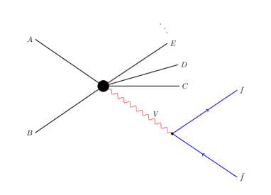
Figure 1: Feynman diagram for a general process for production of spin-$1$ particle ($Z$ boson) and its decay to a pair of fermions

2.1 The production and decay density matrices

We consider a generic reaction $A\ B\to V\ C\ D\ E\ldots$, where particle $V$ is massive and has spin $1$, see Fig. 1. The production density matrix for particle $V$ can be written as

$$\rho(\lambda,\lambda^{\prime})=\frac{\mbox{Phase \ space}}{\mbox{Flux}}\ \mathcal{M}(\lambda)\mathcal{M}^{\dagger}(\lambda^{\prime}).$$ (2)

Here, $\mathcal{M}(\lambda)$ is the helicity amplitude for the production of $V$ with helicity $\lambda\in\{-1,0,1\}$, while the helicities of all the other particles ($A,B,C,D,E\ldots$ ) are suppressed. The differential cross section for the production of $V$ would be given by

$$\dfrac{d\sigma_{V}}{d\Omega_{V}} = \text{Trace}\left[\rho(\lambda,\lambda^{\prime})\right]=\rho(+,+)+\rho(0,0)+\rho(-,-).$$

Here $\Omega_{V}$ is the solid angle of the particle $V$, while the phase space corresponding to all other final state particles is integrated out. The production density matrix can be written in terms of polarization density matrix $P(\lambda,\lambda^{\prime})$ as Boudjema:2009fz

$$P(\lambda,\lambda^{\prime}) = \dfrac{1}{\sigma_{V}}\int\rho(\lambda,\lambda^{\prime})d\Omega_{V}=\dfrac{1}{\sigma_{V}}{\rho}_{T}(\lambda,\lambda^{\prime}).$$ (4)

Here the matrix $P(\lambda,\lambda^{\prime})$ is a $3\times 3$ hermitian matrix that can be parametrized in terms of a vector $\vec{p}=(p_{x},p_{y},p_{z})$ and a symmetric, traceless, second-rank tensor $T_{ij}$ as

$$P(\lambda,\lambda^{\prime})=$$

$$\left[\begin{tabular}[]{lll}$\frac{1}{3}+\frac{p_{z}}{2}+\frac{T_{zz}}{\sqrt{6}}$&$\frac{p_{x}-ip_{y}}{2\sqrt{2}}+\frac{T_{xz}-iT_{yz}}{\sqrt{3}}$&$\frac{T_{xx}-T_{yy}-2iT_{xy}}{\sqrt{6}}$\\ $\frac{p_{x}+ip_{y}}{2\sqrt{2}}+\frac{T_{xz}+iT_{yz}}{\sqrt{3}}$&$\frac{1}{3}-\frac{2T_{zz}}{\sqrt{6}}$&$\frac{p_{x}-ip_{y}}{2\sqrt{2}}-\frac{T_{xz}-iT_{yz}}{\sqrt{3}}$\\ $\frac{T_{xx}-T_{yy}+2iT_{xy}}{\sqrt{6}}$&$\frac{p_{x}+ip_{y}}{2\sqrt{2}}-\frac{T_{xz}+iT_{yz}}{\sqrt{3}}$&$\frac{1}{3}-\frac{p_{z}}{2}+\frac{T_{zz}}{\sqrt{6}}$\end{tabular}\right].$$ (8)

For a spin-$1$ particle decaying to a pair of fermions via the interaction vertex $Vf\bar{f}:\gamma^{\mu}\left(L_{f}\ P_{L}+R_{f}\ P_{R}\right)$, the decay density matrix (normalized to one) is given by Boudjema:2009fz

Here $\theta$, $\phi$ are the polar and the azimuthal orientation of the final state fermion $f$, in the rest frame of $V$ with its would be momentum along $z$-direction. The parameters $\alpha$ and $\delta$ are given by

$$\alpha=\frac{2(R_{f}^{2}-L_{f}^{2})\sqrt{1+(x_{1}^{2}-x_{2}^{2})^{2}-2(x_{1}^{2}+x_{2}^{2})}}{12L_{f}R_{f}x_{1}x_{2}+(R_{f}^{2}+L_{f}^{2})[2-(x_{1}^{2}-x_{2}^{2})^{2}+(x_{1}^{2}+x_{2}^{2})]},$$ (11)

$$\delta=\frac{4L_{f}R_{f}x_{1}x_{2}+(R_{f}^{2}+L_{f}^{2})[(x_{1}^{2}+x_{2}^{2})-(x_{1}^{2}-x_{2}^{2})^{2}]}{12L_{f}R_{f}x_{1}x_{2}+(R_{f}^{2}+L_{f}^{2})[2-(x_{1}^{2}-x_{2}^{2})^{2}+(x_{1}^{2}+x_{2}^{2})]},$$ (12)

with $x_{i}=M_{f}/M_{V}$. For massless final state fermions, $x_{1}\to 0,\ x_{2}\to 0$, one obtains $\delta\to 0$ and $\alpha\to(R_{f}^{2}-L_{f}^{2})/(R_{f}^{2}+L_{f}^{2})$. Combining the production and decay density matrices, the total rate for the process shown in Fig. 1, with particle $V$ being on-shell, is given by Boudjema:2009fz ,

$$\dfrac{1}{\sigma}\dfrac{d\sigma}{d\Omega_{f}}=\frac{2s+1}{4\pi}\sum_{\lambda,\lambda^{\prime}}P(\lambda,\lambda^{\prime})\Gamma(\lambda,\lambda^{\prime}),$$ (13)

where $\sigma=\sigma_{V}BR(V\to f\bar{f})$ is the total cross section for production of $V$ including its decay and $s=1$ being spin of the particle. Using Eqs. (2.1) and (LABEL:decay_density_matrix1) in Eq. (13), the angular distribution for the fermion $f$ becomes

$$\frac{1}{\sigma}\ \frac{d\sigma}{d\Omega_{f}} = \frac{3}{8\pi}\left[\left(\frac{2}{3}-(1-3\delta)\ \frac{T_{zz}}{\sqrt{6}}\right)+\alpha\ p_{z}\cos\theta\right.$$ (14)

$$+ \sqrt{\frac{3}{2}}(1-3\delta)\ T_{zz}\cos^{2}\theta$$

$$+ \left(\alpha\ p_{x}+2\sqrt{\frac{2}{3}}(1-3\delta)\ T_{xz}\cos\theta\right)\sin\theta\ \cos\phi$$

$$+ \left(\alpha\ p_{y}+2\sqrt{\frac{2}{3}}(1-3\delta)\ T_{yz}\cos\theta\right)\sin\theta\ \sin\phi$$

$$+ (1-3\delta)\left(\frac{T_{xx}-T_{yy}}{\sqrt{6}}\right)\sin^{2}\theta\cos(2\phi)$$

$$+ \left.\sqrt{\frac{2}{3}}(1-3\delta)\ T_{xy}\ \sin^{2}\theta\ \sin(2\phi)\right].$$

Using partial integration of this differential distribution of the final state $f$ one can construct several asymmetries to probe various polarization parameters in Eq. (2.1) which will be discussed in the next section.

2.2 Estimation of polarization parameters

For the process of interest, one might want to calculate the polarization parameters of the particle $V$. This can be achieved at two levels: At production process level and at the level of decay products. At the production level we first calculate the production density matrix, Eq. (2), using helicity amplitudes of the production process and then calculate the polarization matrix, Eq. (2.1). The polarization parameters can be extracted from the polarization matrix elements as

$$P_{x}=\frac{\bigg{[}[\rho_{T}(+,0)+\rho_{T}(0,+)]+[\rho_{T}(0,-)+\rho_{T}(-,0)]\bigg{]}}{\sqrt{2}\sigma_{V}},$$

$$P_{y}=\frac{i\bigg{[}[\rho_{T}(0,+)-\rho_{T}(+,0)]+[\rho_{T}(-,0)-\rho_{T}(0,-)]\bigg{]}}{\sqrt{2}\sigma_{V}},$$

$$P_{z}=\dfrac{\bigg{[}\rho_{T}(+,+)-\rho_{T}(-,-)\bigg{]}}{\sigma_{V}},$$

$$T_{xy}=\frac{i\sqrt{6}\bigg{[}\rho_{T}(-,+)-\rho_{T}(+,-)\bigg{]}}{4\sigma_{V}},$$

$$T_{xz}=\frac{\sqrt{3}\bigg{[}[\rho_{T}(+,0)+\rho_{T}(0,+)]-[\rho_{T}(0,-)+\rho_{T}(-,0)]\bigg{]}}{4\sigma_{V}},$$

$$T_{yz}=\frac{i\sqrt{3}\bigg{[}[\rho_{T}(0,+)-\rho_{T}(+,0)]-[\rho_{T}(-,0)-\rho_{T}(0,-)]\bigg{]}}{4\sigma_{V}},$$

$$T_{xx}-T_{yy}=\frac{\sqrt{6}\bigg{[}\rho_{T}(-,+)+\rho_{T}(+,-)\bigg{]}}{2\sigma_{V}},$$

$$T_{zz}=\dfrac{\sqrt{6}}{2}\bigg{[}\frac{\rho_{T}(+,+)+\rho_{T}(-,-)}{\sigma_{V}}-\frac{2}{3}\bigg{]},$$

$$\hskip 14.22636pt=\dfrac{\sqrt{6}}{2}\bigg{[}\frac{1}{3}-\frac{\rho_{T}(0,0)}{\sigma_{V}}\bigg{]}.$$ (15)

Using the tracelessness of $T_{ij}$, $T_{xx}+T_{yy}+T_{zz}=0$, along with values of $T_{zz}$ and $T_{xx}-T_{yy}$ from above, one can calculate $T_{xx}$ and $T_{yy}$ separately.

At the level of decay products, as in a real experiment or in a Monte-Carlo simulator, one needs to compute specific asymmetries to extract the polarization parameters. For example, we can get $P_{x}$ from the left-right asymmetry as

$$A_{x} = \frac{1}{\sigma}\bigg{[}\int_{\theta=0}^{\pi}\int_{\phi=-\frac{\pi}{2}}^{\frac{\pi}{2}}\dfrac{d\sigma}{d\Omega_{f}}d\Omega_{f}-\int_{\theta=0}^{\pi}\int_{\phi=\frac{\pi}{2}}^{3\frac{\pi}{2}}\dfrac{d\sigma}{d\Omega_{f}}d\Omega_{f}\bigg{]}$$ (16)

$$= \frac{3\alpha P_{x}}{4}\equiv\dfrac{\sigma(\cos\phi>0)-\sigma(\cos\phi<0)}{\sigma(\cos\phi>0)+\sigma(\cos\phi<0)}.$$

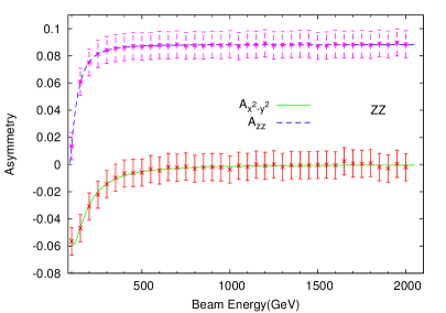
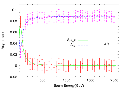
Figure 2: The SM values (analytic) of asymmetries $A_{x^{2}-y^{2}}$ (solid/green line) and $A_{zz}$ (dashed/blue line) as a function of beam energy of the $e^{+}e^{-}$ collider for $ZZ$ (left panel) and $Z\gamma$ (right panel) processes. The data points with error bar corresponds to $10^{4}$ events generated by MadGraph5

All other polarization parameters can be obtained in a similar manner, using Eq. (14):

$$A_{y} \equiv \dfrac{\sigma(\sin\phi>0)-\sigma(\sin\phi<0)}{\sigma(\sin\phi>0)+\sigma(\sin\phi<0)}=\frac{3\alpha P_{y}}{4},$$

$$A_{z} \equiv \dfrac{\sigma(\cos\theta>0)-\sigma(\cos\theta<0)}{\sigma(\cos\theta>0)+\sigma(\cos\theta<0)}=\frac{3\alpha P_{z}}{4},$$

$$A_{xy} \equiv \dfrac{\sigma(\sin 2\phi>0)-\sigma(\sin 2\phi<0)}{\sigma(\sin 2\phi>0)+\sigma(\sin 2\phi<0)}$$

$$= \frac{2}{\pi}\sqrt{\frac{2}{3}}(1-3\delta)T_{xy},$$

$$A_{xz} \equiv \dfrac{\sigma(\cos\theta\cos\phi<0)-\sigma(\cos\theta\cos\phi>0)}{\sigma(\cos\theta\cos\phi>0)+\sigma(\cos\theta\cos\phi<0)}$$

$$= -\frac{2}{\pi}\sqrt{\frac{2}{3}}(1-3\delta)T_{xz},$$

$$A_{yz} \equiv \dfrac{\sigma(\cos\theta\sin\phi>0)-\sigma(\cos\theta\sin\phi<0)}{\sigma(\cos\theta\sin\phi>0)+\sigma(\cos\theta\sin\phi<0)}$$

$$= \frac{2}{\pi}\sqrt{\frac{2}{3}}(1-3\delta)T_{\text{yz}},$$

$$A_{x^{2}-y^{2}} \equiv \dfrac{\sigma(\cos 2\phi>0)-\sigma(\cos 2\phi<0)}{\sigma(\cos 2\phi>0)+\sigma(\cos 2\phi<0)}$$

$$= \frac{1}{\pi}\sqrt{\frac{2}{3}}(1-3\delta)\left(T_{xx}-T_{yy}\right),$$

$$A_{zz} \equiv \dfrac{\sigma(\sin 3\theta>0)-\sigma(\sin 3\theta<0)}{\sigma(\sin 3\theta>0)+\sigma(\sin 3\theta<0)}$$ (17)

$$= \frac{3}{8}\sqrt{\frac{3}{2}}(1-3\delta)T_{zz}.$$

We note that pure azimuthal asymmetries ($A_{x}$, $A_{y}$, $A_{xy}$, $A_{x^{2}-y^{2}}$) listed above were already discussed in Ref. Boudjema:2009fz , however, a complete set of asymmetries for the $W^{\pm}$-boson ($\delta=0,~{}\alpha=-1$) is given in Ref. Aguilar-Saavedra:2015yza .

While extracting the polarization asymmetries in the collider/event generator we have to make sure that the analysis is done in the rest frame of $V$. The initial beam defines the $z$-axis in the lab, while the production plane of $V$ defines the $xz$ plane, i.e. $\phi=0$ plane. While boosting to the rest frame of $V$ we keep the $xz$ plane invariant. The polar and the azimuthal angles of the decay products of $V$ are measured with respect to the would-be momentum of $V$.

As a demonstration of the two methods mentioned above, we look at two processes: $e^{+}e^{-}\to~{}ZZ$ and $e^{+}e^{-}\to~{}Z\gamma$. The polarization parameters are constructed both at the production level, using Eq. (2.2), and at the decay level, using Eqs. (16) and (2.2). We observe that out of eight polarization asymmetries only three, $A_{x}$, $A_{x^{2}-y^{2}}$, and $A_{zz}$, are non-zero in the SM. The asymmetries $A_{x^{2}-y^{2}}$ and $A_{zz}$ are calculated analytically for the production part and shown as a function of beam energy in Fig. 2 with solid lines. For the same processes with $Z\to f\bar{f}$ decay, we generate events using MadGraph5 Alwall:2014hca with different values of beam energies. The polarization asymmetries were constructed from these events and are shown in Fig. 2 with points. The statistical error bars shown correspond to $10^{4}$ events. We observe agreement between the asymmetries calculated at the production level (analytically) and the decay level (using event generator). Any possible new physics in the production process of $Z$ boson is expected to change the cross section, kinematical distributions and the values of the polarization parameters/asymmetries. We intend to use these asymmetries to probe the standard and BSM physics.

3 Anomalous Lagrangian and their probes

The effective Lagrangian for the anomalous trilinear gauge boson interactions in the neutral sector is given in Eq. (LABEL:LaTGCfull), which includes both dimension-$6$ and dimension-$8$ operators as found in the literature. For the present work we restrict our analysis to dimension-$6$ operators only. Thus, the anomalous Lagrangian of our interest is

$${\cal L}_{aTGC}^{dim-6} = \frac{g_{e}}{M_{Z}^{2}}\Bigg{[}-[f_{4}^{\gamma}(\partial_{\mu}F^{\mu\beta})+f_{4}^{Z}(\partial_{\mu}Z^{\mu\beta})]Z_{\alpha}(\partial^{\alpha}Z_{\beta})$$ (18)

$$+ [f_{5}^{\gamma}(\partial^{\sigma}F_{\sigma\mu})+f_{5}^{Z}(\partial^{\sigma}Z_{\sigma\mu})]\widetilde{Z}^{\mu\beta}Z_{\beta}$$

$$- [h_{1}^{\gamma}(\partial^{\sigma}F_{\sigma\mu})+h_{1}^{Z}(\partial^{\sigma}Z_{\sigma\mu})]Z_{\beta}F^{\mu\beta}$$

$$- [h_{3}^{\gamma}(\partial_{\sigma}F^{\sigma\rho})+h_{3}^{Z}(\partial_{\sigma}Z^{\sigma\rho})]Z^{\alpha}\widetilde{F}_{\rho\alpha}\Bigg{]}.$$

This yields anomalous vertices $ZZZ$ through $f^{Z}_{4,5}$ couplings, $\gamma ZZ$ through $f^{\gamma}_{4,5}$ and $h^{Z}_{1,3}$ couplings and $\gamma\gamma Z$ through $h^{\gamma}_{1,3}$ couplings. There is no $\gamma\gamma\gamma$ vertex in the above Lagrangian.

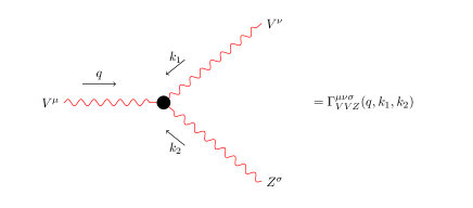
Figure 3: Feynman diagram for a general anomalous triple gauge boson vertex with $V=Z/\gamma$

We use FeynRules Alloul:2013bka to obtain the vertex tensors and they are given by

$$\Gamma_{\gamma ZZ}^{\mu\nu\sigma}(q,k_{1},k_{2})=$$

$$\dfrac{g_{e}}{M_{Z}^{2}}\Bigg{[}f_{4}^{\gamma}\bigg{(}\left(k_{2}^{\nu}g^{\mu\sigma}+k_{1}^{\sigma}g^{\mu\nu}\right)q^{2}-q^{\mu}\left(k_{1}^{\sigma}q^{\nu}+k_{2}^{\nu}q^{\sigma}\right)\bigg{)}\Bigg{.}$$

$$+f_{5}^{\gamma}\left(q^{\mu}{q}_{\beta}\epsilon^{\nu\sigma\alpha\beta}+q^{2}\epsilon^{\mu\nu\sigma\alpha}\right)(k_{1}-k_{2})_{\alpha}$$

$$+h_{1}^{Z}\bigg{(}k_{2}^{\mu}q^{\nu}k_{2}^{\sigma}+k_{1}^{\mu}k_{1}^{\nu}q^{\sigma}+\left(k_{1}^{2}-k_{2}^{2}\right)\left(q^{\nu}g^{\mu\sigma}-q^{\sigma}g^{\mu\nu}\right)\bigg{.}$$

$$\bigg{.}-k_{2}^{\sigma}g^{\mu\nu}q.k_{2}-k_{1}^{\nu}g^{\mu\sigma}q.k_{1}\bigg{)}$$

$$\Bigg{.}-h_{3}^{Z}\left(k_{1}^{\nu}{k_{1}}_{\beta}\epsilon^{\mu\sigma\alpha\beta}+{k_{2}}_{\beta}k_{2}^{\sigma}\epsilon^{\mu\nu\alpha\beta}+\left(k_{2}^{2}-k_{1}^{2}\right)\epsilon^{\mu\nu\sigma\alpha}\right){q}_{\alpha}\Bigg{]},$$

$$\Gamma_{ZZZ}^{\mu\nu\sigma}(q,k_{1},k_{2})=$$

$$\dfrac{g_{e}}{M_{Z}^{2}}\Bigg{[}f_{4}^{Z}\bigg{(}-q^{\mu}q^{\nu}k_{1}^{\sigma}-k_{2}^{\mu}q^{\nu}k_{2}^{\sigma}-k_{2}^{\mu}k_{1}^{\nu}k_{1}^{\sigma}-k_{1}^{\mu}k_{2}^{\nu}k_{2}^{\sigma}\bigg{.}\Bigg{.}$$

$$-\left(q^{\mu}k_{2}^{\nu}+k_{1}^{\mu}k_{1}^{\nu}\right)q^{\sigma}+g^{\mu\nu}\left(q^{2}k_{1}^{\sigma}+k_{1}^{2}q^{\sigma}\right)$$

$$\bigg{.}+g^{\mu\sigma}\left(q^{2}k_{2}^{\nu}+k_{2}^{2}q^{\nu}\right)+g^{\nu\sigma}\left(k_{2}^{2}k_{1}^{\mu}+k_{1}^{2}k_{2}^{\mu}\right)\bigg{)}$$

$$-f_{5}^{Z}\bigg{(}\epsilon^{\mu\nu\alpha\beta}(k_{1}-q)_{\alpha}{k_{2}}_{\beta}k_{2}^{\sigma}+\epsilon^{\mu\nu\sigma\alpha}\left(\left(k_{1}^{2}-k_{2}^{2}\right){q}_{\alpha}\right.\bigg{.}$$

$$\left.+\left(k_{2}^{2}-q^{2}\right){k_{1}}_{\alpha}+\left(q^{2}-k_{1}^{2}\right){k_{2}}_{\alpha}\right)$$

$$\Bigg{.}\bigg{.}+{k_{1}}_{\beta}k_{1}^{\nu}(k_{2}-q)_{\alpha}\epsilon^{\mu\sigma\alpha\beta}+{q}_{\beta}q^{\mu}(k_{2}-k_{1})_{\alpha}\epsilon^{\nu\sigma\alpha\beta}\bigg{)}\Bigg{]},$$

$$\Gamma_{\gamma\gamma Z}^{\mu\nu\sigma}(q,k_{1},k_{2})=$$

$$\dfrac{g_{e}}{M_{Z}^{2}}\Bigg{[}h_{1}^{\gamma}\bigg{(}q^{\mu}q^{\nu}k_{1}^{\sigma}+q^{\sigma}k_{1}^{\mu}k_{1}^{\nu}-g^{\mu\nu}\left(q^{2}k_{1}^{\sigma}+k_{1}^{2}q^{\sigma}\right)\Bigg{.}\bigg{.}$$

$$\bigg{.}+g^{\mu\sigma}\left(k_{1}^{2}q^{\nu}-q.k_{1}k_{1}^{\nu}\right)+g^{\nu\sigma}\left(q^{2}k_{1}^{\mu}-q.k_{1}q^{\mu}\right)\bigg{)}$$

$$-h_{3}^{\gamma}\bigg{(}{k_{1}}_{\beta}k_{1}^{\nu}{q}_{\alpha}\epsilon^{\mu\sigma\alpha\beta}+q^{\mu}{k_{1}}_{\alpha}{q}_{\beta}\epsilon^{\nu\sigma\alpha\beta}\bigg{.}$$

$$+\Bigg{.}\bigg{.}\left(q^{2}{k_{1}}_{\alpha}-k_{1}^{2}{q}_{\alpha}\right)\epsilon^{\mu\nu\sigma\alpha}\bigg{)}\Bigg{]}.$$ (21)

The notations for momentum and Lorentz indices are shown in Fig. 3. We are interested in possible trilinear gauge boson vertices appearing in the processes $e^{+}e^{-}\to ZZ$ and $e^{+}e^{-}\to Z\gamma$ with final state gauge bosons being on-shell. For the process $e^{+}e^{-}\to ZZ$, the vertices $\gamma^{\star}ZZ$ and $Z^{\star}ZZ$ appear with on-shell conditions $k_{1}^{2}=k_{2}^{2}=M_{Z}^{2}$. The terms proportional to $k_{1}^{\nu}$ and $k_{2}^{\sigma}$ in Eqs. (3) and (3) vanish due to the transversity of the polarization states. Thus, in the on-shell case, the vertices for $e^{+}e^{-}\to ZZ$ reduce to

$$\Gamma_{V^{\star}ZZ}^{\mu\nu\sigma}(q,k_{1},k_{2})= -\dfrac{g_{e}}{M_{Z}^{2}}\left(q^{2}-M_{V}^{2}\right)\Bigg{[}f_{4}^{V}\left(q^{\sigma}g^{\mu\nu}+q^{\nu}g^{\mu\sigma}\right)\Bigg{.}$$ (22)

$$\Bigg{.}-f_{5}^{V}\epsilon^{\mu\nu\sigma\alpha}(k_{1}-k_{2})_{\alpha}\Bigg{]}.$$

For the process $e^{+}e^{-}\to Z\gamma$ the vertices $\gamma Z^{\star}Z$ and $\gamma^{\star}\gamma Z$ appear with corresponding on-shell and polarization transversity conditions. Putting these conditions in Eqs. (3) and (3) and some relabelling of momenta etc. in Eq. (3) the relevant vertices $Z^{\star}\gamma Z$ and $\gamma^{\star}\gamma Z$ can be represented together by

$$\Gamma_{V^{\star}\gamma Z}^{\mu\nu\sigma}(q,k_{1},k_{2})= \dfrac{g_{e}}{M_{Z}^{2}}\left(q^{2}-M_{V}^{2}\right)\Bigg{[}h_{1}^{V}\left(k_{1}^{\mu}g^{\nu\sigma}-k_{1}^{\sigma}g^{\mu\nu}\right)$$ (23)

$$-h_{3}^{V}\epsilon^{\mu\nu\sigma\alpha}{k_{1}}_{\alpha}\Bigg{]}.$$

The off-shell $V^{\star}$ is the propagator in our processes and couples to the massless electron current, as shown in Fig. 4(c), (d). After above-mentioned reduction of the vertices, there were some terms proportional to $q^{\mu}$ that yield zero upon contraction with the electron current, hence they are dropped from the above expressions. We note that although $h^{Z}$ and $f^{\gamma}$ appear together in the off-shell vertex of $\gamma ZZ$ in Eq. (3), they decouple after choosing separate processes; the $f^{V}$ appear only in $e^{+}e^{-}\to ZZ$, while the $h^{V}$ appear only in $e^{+}e^{-}\to Z\gamma$. This decoupling simplifies our analysis as we can study two processes independent of each other when we perform a global fit to the parameters in Section 5.

4 Asymmetries, limits, and sensitivity to anomalous couplings

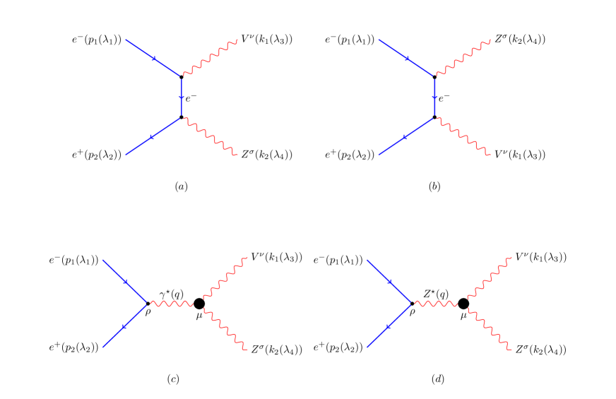
Figure 4: Feynman diagrams for the production of $ZZ$ or $Z\gamma$ at $e^{+}e^{-}$ collider

In this section we thoroughly investigate the effects of anomalous couplings in the processes $e^{+}e^{-}\to ZZ$ and $e^{+}e^{-}\to Z\gamma$. We use tree level SM interactions along-with anomalous couplings shown in Eq. (18) for our analysis. The Feynman diagrams for these processes are given in the Fig. 4 where the anomalous vertices are shown as big blobs. The helicity amplitudes for the anomalous part together with SM contributions for both these processes are given in A. These are then used to calculate the polarization observables and the cross section which are given in B.

4.1 Parametric dependence of asymmetries on anomalous couplings

The dependences of the observables on the anomalous couplings for the $ZZ$ and $Z\gamma$ processes are given in Tables 2 and 3, respectively.

Table 2: Dependence of the polarization observables on the anomalous coupling in $ZZ$ final state

Observables	Linear terms	Quadratic terms
$\sigma$	$f_{5}^{Z},f_{5}^{\gamma}$	$(f_{4}^{\gamma})^{2},(f_{5}^{\gamma})^{2},(f_{4}^{Z})^{2},(f_{5}^{Z})^{2},f_{4}^{\gamma}f_{4}^{Z},f_{5}^{\gamma}f_{5}^{Z}$
$\sigma\times A_{x}$	$f_{5}^{\gamma},f_{5}^{Z}$	$-$
$\sigma\times A_{y}$	$f_{4}^{\gamma},f_{4}^{Z}$	$-$
$\sigma\times A_{xy}$	$f_{4}^{Z},f_{4}^{\gamma}$	$f_{4}^{Z}f_{5}^{\gamma},f_{4}^{\gamma}f_{5}^{Z},f_{4}^{\gamma}f_{5}^{\gamma},f_{4}^{Z}f_{5}^{Z}$
$\sigma\times A_{x^{2}-y^{2}}$	$f_{5}^{Z},f_{5}^{\gamma}$	$(f_{4}^{\gamma})^{2},(f_{5}^{\gamma})^{2},(f_{4}^{Z})^{2},(f_{5}^{Z})^{2},f_{4}^{\gamma}f_{4}^{Z},f_{5}^{\gamma}f_{5}^{Z}$
$\sigma\times A_{zz}$	$f_{5}^{Z},f_{5}^{\gamma}$	$(f_{4}^{\gamma})^{2},(f_{5}^{\gamma})^{2},(f_{4}^{Z})^{2},(f_{5}^{Z})^{2},f_{4}^{\gamma}f_{4}^{Z},f_{5}^{\gamma}f_{5}^{Z}$

Table 3: Dependence of the polarization observables on the anomalous coupling in $Z\gamma$ final state

Observables	Linear terms	Quadratic terms
$\sigma$	$h_{3}^{Z},h_{3}^{\gamma}$	$(h_{1}^{\gamma})^{2},(h_{3}^{\gamma})^{2},(h_{1}^{Z})^{2},(h_{3}^{Z})^{2},h_{1}^{\gamma}h_{1}^{Z},h_{3}^{\gamma}h_{3}^{Z}$
$\sigma\times A_{x}$	$h_{3}^{Z},h_{3}^{\gamma}$	$(h_{1}^{\gamma})^{2},(h_{3}^{\gamma})^{2},(h_{1}^{Z})^{2},(h_{3}^{Z})^{2},h_{1}^{\gamma}h_{1}^{Z},h_{3}^{\gamma}h_{3}^{Z}$
$\sigma\times A_{y}$	$h_{1}^{\gamma},h_{1}^{Z}$	$-$
$\sigma\times A_{xy}$	$h_{1}^{\gamma},h_{1}^{Z}$	$-$
$\sigma\times A_{x^{2}-y^{2}}$	$h_{3}^{\gamma},h_{3}^{Z}$	$-$
$\sigma\times A_{zz}$	$h_{3}^{Z},h_{3}^{\gamma}$	$(h_{1}^{\gamma})^{2},(h_{3}^{\gamma})^{2},(h_{1}^{Z})^{2},(h_{3}^{Z})^{2},h_{1}^{\gamma}h_{1}^{Z},h_{3}^{\gamma}h_{3}^{Z}$

In the SM, the helicity amplitudes are real, thus the production density matrix elements in Eq. (2) are all real. This implies $A_{y}$, $A_{xy}$ and $A_{yz}$ are all zero in the SM: see Eq. (2.2). The asymmetries $A_{z}$ and $A_{xz}$ are also zero for the SM couplings due to the forward-backward symmetry of the $Z$ boson in the c.m. frame, owing to the presence of both $t$- and $u$-channel diagrams and unpolarized initial beams. After including anomalous couplings, $A_{y}$ and $A_{xy}$ receive a non-zero contribution, while $A_{z}$, $A_{xz}$ and $A_{yz}$ remain zero for the unpolarized initial beams.

From the list of non-vanishing asymmetries, only $A_{y}$ and $A_{xy}$ are CP-odd, while the others are CP-even. All the CP-odd observables are linearly dependent upon the CP-odd couplings, like $f_{4}^{V}$ and $h_{1}^{V}$, while all the CP-even observables have only quadratic dependence on the CP-odd couplings. In the SM, the $Z$ boson’s couplings respect CP symmetry; thus $A_{y}$ and $A_{xy}$ vanish. Hence, any significant deviation of $A_{y}$ and $A_{xy}$ from zero at the collider will indicate a clear sign of CP-violating new physics interactions. Observables that have only a linear dependence on the anomalous couplings yield a single interval limits on these couplings. On the other hand, any quadratic appearance (like $(f_{5}^{V})^{2}$ in $\sigma$) may yield more than one interval of the couplings, while putting limits. For the case of $ZZ$ process, $A_{x}$ and $A_{y}$ do not have any quadratic dependence, hence they yield the cleanest limits on the CP-even and -odd parameters, respectively. Similarly, for the $Z\gamma$ process we have $A_{y}$, $A_{xy}$, and $A_{x^{2}-y^{2}}$, which have only a linear dependence and provide clean limits. These clean limits, however, may not be the strongest limits as we will see in the following sections.

4.2 Sensitivity and limits on anomalous couplings

Sensitivity of an observable $\mathcal{O}$ dependent on parameter $\vec{f}$ is defined as

$${\cal S}(\mathcal{O}(\vec{f}))=\dfrac{|\mathcal{O}(\vec{f})-\mathcal{O}(\vec{f}=0)|}{\delta\mathcal{O}},$$ (24)

where $\delta\mathcal{O}=\sqrt{(\delta\mathcal{O}_{stat.})^{2}+(\delta\mathcal{O}_{sys.})^{2}}$ is the estimated error in $\mathcal{O}$. If the observable is an asymmetry, $A=(N^{+}-N^{-})/(N^{+}+N^{-})$, the error is given by

$$\delta A=\sqrt{\frac{1-A^{2}}{{\cal L}\sigma}+\epsilon_{A}^{2}},$$ (25)

where $N^{+}+N^{-}=N_{T}=L\sigma$, ${\cal L}$ being the integrated luminosity of the collider. The error in the cross section $\sigma$ will be given by

$$\delta\sigma=\sqrt{\frac{\sigma}{{\cal L}}+(\epsilon\sigma)^{2}}.$$ (26)

Here $\epsilon_{A}$ and $\epsilon$ are the systematic fractional errors in $A$ and $\sigma$, respectively, while remaining one are statistical errors.

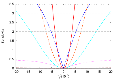
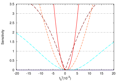
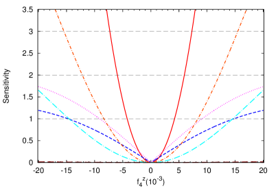
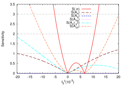
Figure 5: Sensitivity of the cross section and asymmetries to anomalous couplings for the process $e^{+}e^{-}\rightarrow ZZ$ with $\sqrt{\hat{s}}=500$ GeV and $L=100$ fb^-1

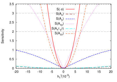
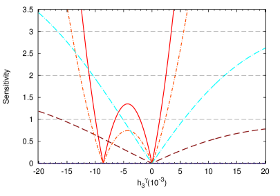
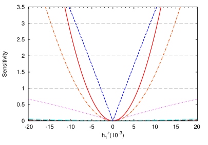
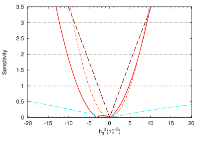
Figure 6: Sensitivity of the cross section and asymmetries to anomalous couplings for the process $e^{+}e^{-}\rightarrow Z\gamma$ with $\sqrt{\hat{s}}=500$ GeV, $L=100$ fb^-1, and $10^{\circ}\leq\theta_{\gamma}\leq 170^{\circ}$

For numerical calculations, we choose ILC running at c.m. energy $\sqrt{\hat{s}}=500$ GeV and integrated luminosity ${\cal L}=100$ fb^-1. We use $\epsilon_{A}=\epsilon=0$ for most of our analysis, however, we do discuss the impact of systematic errors on our results. With this choice the sensitivity of all the polarization asymmetries, Eq. (2.2), and the cross section have been calculated varying one parameter at a time. These sensitivities are shown in Figs. 5 and 6 for the $ZZ$ and $Z\gamma$ processes, respectively, for each observable. In the $e^{+}e^{-}\to Z\gamma$ process we have taken a cut-off on the polar angle, $10^{\circ}\leq\theta_{\gamma}\leq 170^{\circ}$ to keep away from the beam pipe. For these limits the analytical expressions shown in B are used.

We see that in the $ZZ$ process the tightest constraint on $f_{4}^{\gamma}$ at $1\sigma$ level comes from the asymmetry $A_{y}$ owing to its linear and strong dependence on the coupling. For $f_{5}^{\gamma}$, both $A_{x}$ and the cross section $\sigma_{ZZ}$, give comparable limits at $1\sigma$ but $\sigma_{ZZ}$ gives a tighter limit at higher values of sensitivity. This is because the quadratic term in $\sigma_{ZZ}$ comes with higher power of energy/momenta and hence a larger sensitivity. Similarly, the strongest limit on $f_{4}^{Z}$ and $f_{5}^{Z}$ as well comes from $\sigma_{ZZ}$. Though the cross section gives the tightest constrain on most of the coupling in $ZZ$ process, our polarization asymmetries also provide comparable limits. Another noticeable fact is that $\sigma_{ZZ}$ has a linear as well as quadratic dependence on $f_{5}^{Z}$ and the sensitivity curve is symmetric about a point larger than zero. Thus, when we do a parameter estimation exercise, we will always have a bias toward a positive value of $f_{5}^{Z}$. The same is the case with the coupling $f_{5}^{\gamma}$ , but the strength of the linear term is small and the sensitivity plot with $\sigma_{ZZ}$ looks almost symmetric about $f_{5}^{\gamma}=0$.

In the $Z\gamma$ process, the tightest constraint on $h_{1}^{\gamma}$ comes from $A_{xy}$, on $h_{3}^{\gamma}$ it comes from $\sigma_{Z\gamma}$, on it $h_{1}^{Z}$ comes from $A_{y}$, and on $h_{3}^{Z}$ it comes from $A_{x}$. The cross section $\sigma_{Z\gamma}$ and $A_{zz}$ has a linear as well as quadratic dependence on $h_{3}^{\gamma}$, and $\sigma_{Z\gamma}$ and they give two intervals at $1\sigma$ level. Other observables can help resolve the degeneracy when we use more than one observables at a time. Still, the cross section prefers a negative value of $h_{3}^{\gamma}$ and it will be seen again in a multi-variate analysis. The coupling $h_{3}^{Z}$ also has quadratic appearance in the cross section and yields a bias toward negative values of $h_{3}^{Z}$.

Table 4: List of tightest limits on anomalous couplings at $1~{}\sigma$ level and the corresponding observable obtained for $\sqrt{\hat{s}}=500$ GeV and $L=100$ fb^-1

$ZZ$ process			$Z\gamma$ process
Coupling	Limits	Comes from	Coupling	Limits	Comes from
$|f_{4}^{\gamma}|$	$\leq 2.4\times 10^{-3}$	$A_{y}$	$|h_{1}^{\gamma}|$	$\leq 3.6\times 10^{-3}$	$A_{xy}$, $\sigma$
$|f_{4}^{Z}|$	$\leq 4.2\times 10^{-3}$	$\sigma$	$|h_{1}^{Z}|$	$\leq 2.9\times 10^{-3}$	$A_{y}$
$f_{5}^{\gamma}$	$\in[-2.3,2.7]\times 10^{-3}$	$A_{x}$, $\sigma$	$h_{3}^{\gamma}$	$\in[-2.1,1.3]\times 10^{-3}$	$\sigma$
				or $\in[-9.9,-6.5]\times 10^{-3}$
$f_{5}^{Z}$	$\in[-2.3,8.8]\times 10^{-3}$	$\sigma$	$|h_{3}^{Z}|$	$\leq 2.8\times 10^{-3}$	$A_{x}$

The tightest limits on the anomalous couplings (at $1\sigma$ level), obtained using one observable at a time and varying one coupling at a time, are listed in Table 4 along with the corresponding observables. A comparison between Tables 1 and 4 shows that an $e^{+}e^{-}$ collider running at $500$ GeV and $100$ fb^-1 provides better limits on the anomalous coupling ($f_{i}^{V}$) in the $ZZ$ process than the $7$ TeV LHC at $5$ fb^-1. For the $Z\gamma$ process the experimental limits are available from $8$ TeV LHC with $19.6$ fb^-1 luminosity (Table 1) and they are comparable to the single observable limits shown in Table 4. These limits can be further improved if we use all the observables in a $\chi^{2}$ kind of analysis.

We can further see that the sensitivity curves for CP-odd observables, $A_{y}$ and $A_{xy}$, has no or a very mild dependence on the CP-even couplings. The mild dependence comes through the cross section $\sigma$, sitting in the denominator of the asymmetries. We see that CP-even observables provide tight constraint on CP-even couplings and CP-odd observables provide tight constraint on the CP-odd couplings. Thus, not only can we study the two processes independently, it is possible to study the CP-even and CP-odd couplings almost independent of each other. To this end, we shall perform a two-parameter sensitivity analysis in the next subsection.

A note on the systematic error is in order. The sensitivity of an observable is inversely proportional to the size of its estimated error, Eq. (24). Including the systematic error will increase the size of the estimated error and hence decrease the sensitivity. For example, including $\epsilon_{A}=1~{}\%$ to $L=100$ fb^-1 increases $\delta A$ by a factor of $1.3$ and dilutes the sensitivity by the same factor. This modifies the best limit on $|f_{4}^{\gamma}|$, coming from $A_{y}$, to $2.97\times 10^{-3}$ (dilution by a factor of $1.3$); see Table 4. For the cross section, adding $\epsilon=2~{}\%$ systematic error increases $\delta\sigma$ by a factor of $1.5$. The best limit on $|f_{4}^{Z}|$, coming from the cross section, changes to $5.35\times 10^{-3}$, a dilution by a factor of $1.2$. Since inclusion of the above systematic errors modifies the limits on the couplings only by $20~{}\%$ to $30~{}\%$, we shall restrict ourselves to the statistical error for simplicity for rest of the analysis.

4.3 Two-parameter sensitivity analysis

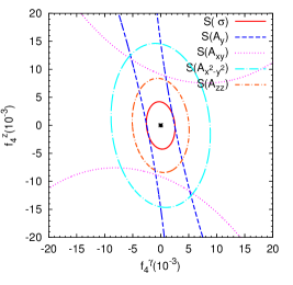
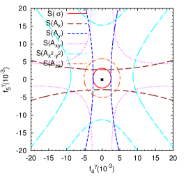
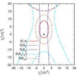
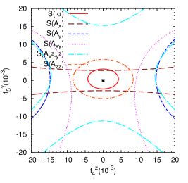
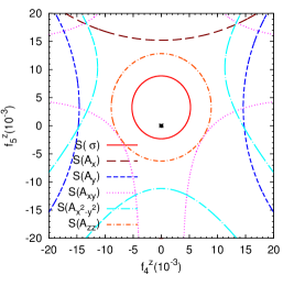
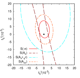
Figure 7: $1\sigma$ sensitivity contours ($\Delta\chi^{2}=1$) for cross section and asymmetries obtained by varying two parameters at a time and keeping the others at zero for the $ZZ$ process at $\sqrt{\hat{s}}=500$ GeV and $L=100$ fb^-1

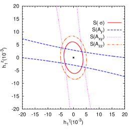
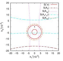
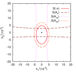
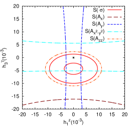
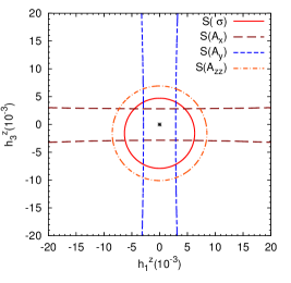
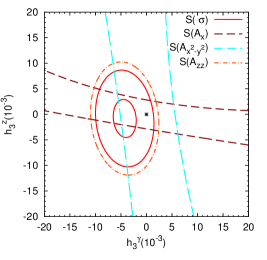
Figure 8: $1\sigma$ sensitivity contours ($\Delta\chi^{2}=1$) for cross section and asymmetries obtained by varying two parameters at a time and keeping the others at zero for the $Z\gamma$ process at $\sqrt{\hat{s}}=500$ GeV, $L=100$ fb^-1, and $10^{\circ}\leq\theta_{\gamma}\leq 170^{\circ}$

We vary two couplings at a time, for each observable, and plot the ${\cal S}=1$ (or $\Delta\chi^{2}=1$) contours in the corresponding parameter plane. These contours are shown in Fig. 7 and Fig. 8 for $ZZ$ and $Z\gamma$ processes, respectively. Asterisk ($\star$) marks in the middle of these plots denote the SM value, i.e., the $(0,0)$ point. Each panel corresponds to two couplings that are varied and all others are kept at zero. The shapes of the contours, for a given observable, are a reflection of its dependence on the couplings as shown in Tables 2 and 3. For example, let us look at the middle-top panel of Fig. 7, i.e. the $(f_{4}^{\gamma}-f_{5}^{\gamma})$ plane. The contours corresponding to the cross section (solid/red) and $A_{zz}$ (short-dash-dotted/orange) are circular in shape due to their quadratic dependence on these two couplings with the same sign. The small linear dependence on $f_{5}^{\gamma}$ makes these circles move toward a small positive value, as already observed in the one-parameter analysis above. The $A_{y}$ contour (short-dash/blue) depends only on $f_{4}^{\gamma}$ in the numerator and a mild dependence on $f_{5}^{\gamma}$ enters through the cross section, sitting in the denominator of the asymmetries. The role of two couplings are exchanged for the $A_{x}$ contour (big-dash/black). The $A_{xy}$ contour (dotted/magenta) is hyperbolic in shape, indicating a dependence on the product $f_{4}^{\gamma}f_{5}^{\gamma}$, while a small shift toward positive $f_{5}^{\gamma}$ value indicates a linear dependence on it. Similarly the symmetry about $f_{4}^{\gamma}=0$ indicates no linear dependence on it for $A_{xy}$. All these observations can be confirmed by looking at Table 2 and the expressions in B. Finally, the shape of the $A_{x^{2}-y^{2}}$ contour (big-dash-dotted/cyan) indicates a quadratic dependence on two couplings with opposite sign. Similarly, all other panels can be read. Note that taking any one of the coupling to zero in these panels gives us the $1\sigma$ limit on the other couplings as found in the one-parameter analysis above.

In the contours for the $Z\gamma$ process, Fig. 8, one new kind of shape appears: the annular ring corresponding to $\sigma_{Z\gamma}$ in middle-top, left-bottom, and right-bottom panels. This shape corresponds to a large linear dependence of the cross section on $h_{3}^{\gamma}$ along with the quadratic dependence. By putting the other couplings to zero in above-mentioned panels one obtains two disjoint internals for $h_{3}^{\gamma}$ at $1\sigma$ level as found before in the one-parameter analysis. The plane containing two CP-odd couplings, i.e. the left-top panel, has two sets of slanted contours corresponding to $A_{y}$ (short-dash/blue) and $A_{xy}$ (dotted/magenta), the CP-odd observables. These observables depend upon both the couplings linearly and hence the slanted (almost) parallel lines. The rest of the panels can be read in the same way.

Till here we have used only one observable at a time for finding the limits. A combination of all the observables would provide a much tighter limit on the couplings than provided by any one of them alone. Also, the shape, the position, and the orientation of the allowed region would change if the other two parameters were set to some value other than zero. A more comprehensive analysis requires varying all the parameters and using all the observables to find the parameter region of low $\chi^{2}$ or high likelihood. The likelihood mapping of the parameter space is performed using the MCMC method in the next section.

5 Likelihood mapping of parameter space

In this section we perform a mock analysis of parameter estimation of anomalous coupling using pseudo data generated by MadGraph5. We choose two benchmark points for coupling parameters as follows:

SM $$: f_{4,5}^{V}=0.000,\ \ h_{1,3}^{V}=0.000\ \ \mbox{and}$$

aTGC $$: f_{4,5}^{V}=0.005,\ \ h_{1,3}^{V}=0.005\ .$$ (27)

For each of these benchmark points we generate events in MadGraph5 for pseudo data corresponding to ILC running at $500$ GeV and integrated luminosity of $L=100$ fb^-1. The likelihood of a given point $\vec{f}$ in the parameter space is defined by

$${\cal L}(\vec{f})=\prod_{i}\exp\left[-\ \frac{\left({\cal O}_{i}(\vec{f})-{\cal O}_{i}(\vec{f}_{0})\right)^{2}}{2\left(\delta{\cal O}_{i}(\vec{f}_{0})\right)^{2}}\right],$$ (28)

where $\vec{f}_{0}$ defines the benchmark point. The product runs over the list of observables we have: the cross section and five non-zero asymmetries. We use the MCMC method to map the likelihood of the parameter space for each of the benchmark point and for both processes. The one-dimensional marginalized distributions and the two-dimensional contours on the anomalous couplings are drawn from the Markov chains using the GetDist package Antony:GetDist .

5.1 MCMC analysis for $e^{+}e^{-}\to ZZ$

Here we look at the process $e^{+}e^{-}\to ZZ$ followed by the decays $Z\to l^{+}l^{-}$ and $Z\to q\bar{q}$, with $l^{-}=e^{-},~{}\mu^{-}$ in the
MadGraph5 simulations. The total cross section for this whole process would be

$$\sigma=\sigma(e^{+}e^{-}\to ZZ)\times 2\ Br(Z\to l^{+}l^{-})\ Br(Z\to q\bar{q}).$$ (29)

The theoretical values of $\sigma(e^{+}e^{-}\to ZZ)$ and all the asymmetries are obtained using expressions given in Appendix B and shown in the second column of Tables 5 and 6 for benchmark points SM and aTGC, respectively. The MadGraph5 simulated values for these observables are given in the third column of the two tables mentioned for two benchmark points. Using these simulated values as pseudo data we perform the likelihood mapping of the parameter space and obtain the posterior distributions for parameters and the observables. The last two columns of Tables 5 and 6 show the 68 % and 95 % Bayesian confidence interval (BCI) of the observables used. One naively expects 68 % BCI to roughly have the same size as the $1\sigma$ error in the pseudo data. However, we note that the 68 % BCI for all the asymmetries is much narrower than expected, for both benchmark points. This can be understood from the fact that the cross section provides the strongest limit on any parameter, as noticed in the earlier section, thus limiting the range of values for the asymmetries. However, this must allow 68 % BCI of the cross section to match with the expectation. This indeed happens for the aTGC case (Table 6), but for the SM case even the cross section is narrowly constrained compared to a naive expectation. The reason for this can be found in the dependence of the cross section on the parameters. For most of the parameter space, the cross section is larger than the SM prediction and only for a small range of parameter space it can be smaller. This was already pointed out while discussing multi-valued sensitivity in Fig. 5. We found the lowest possible value of the cross section to be $37.77$ fb, obtained for $f_{4}^{\gamma,Z}\approx 0$, $f_{5}^{\gamma}\sim 2\times 10^{-4}$, and $f_{5}^{Z}\sim 3.2\times 10^{-3}$.

Table 5: List of observables shown for the process $e^{+}e^{-}\to ZZ$ for the benchmark point SM with $\sqrt{\hat{s}}=500$ GeV: theoretical values (column 2), MadGraph5 simulated value for $L=100$ fb^-1 (column 3), 68 % (column 4) and 95 % (column 5) Bayesian confidence intervals (BCI)

Observables	Theoretical (SM)	MadGraph (SM, prior)	68 % BCI (posterior)	95 % BCI (posterior)
$\sigma$	$38.096$ fb	$38.16\pm 0.62$ fb	$38.61^{+0.31}_{-0.53}$fb	$38.61^{0.83}_{-0.74}$fb
$A_{x}$	$0.00099$	$0.0023\pm 0.0161$	$-0.0021\pm 0.0087$	$-0.0021^{+0.016}_{-0.017}$
$A_{y}$	$0$	$-0.0016\pm 0.0161$	$-0.0005\pm 0.0090$	$-0.0005^{+0.017}_{-0.017}$
$A_{xy}$	$0$	$0.0004\pm 0.0161$	$0.0001\pm 0.0036$	$0.0001^{+0.0071}_{-0.0071}$
$A_{x^{2}-y^{2}}$	$-0.02005$	$-0.0189\pm 0.0161$	$-0.0166^{+0.0032}_{-0.0018}$	$-0.0166^{+0.0043}_{-0.0052}$
$A_{zz}$	$0.17262$	$0.1745\pm 0.0159$	$0.1691^{+0.0035}_{-0.0022}$	$0.1691^{+0.0051}_{-0.0056}$

Thus, for most of the parameter space the anomalous couplings cannot emulate the negative statistical fluctuations in the cross section making the likelihood function, effectively, a one-sided Gaussian function. This forces the mean of posterior distribution to a higher value. We also note that the upper bound of the 68 % BCI for cross section ($38.92$ fb) is comparable to the expected $1\sigma$ upper bound ($38.78$ fb). Thus we have an overall narrowing of the range of the posterior distribution of the cross section values. This, in turns, leads to a narrow range of parameters allowed and hence narrow ranges for the asymmetries in the case of SM benchmark point. For the aTGC benchmark point, it is possible to emulate the negative fluctuations in cross section by varying the parameters, thus the corresponding posterior distributions compare with the expected $1\sigma$ fluctuations. The narrow ranges for the posterior distribution for all the asymmetries are due to the tighter constraints on the parameters coming from the cross section and correlation between the observables.

Table 6: List of observables shown for the process $e^{+}e^{-}\to ZZ$ for the benchmark point aTGC with $\sqrt{\hat{s}}=500$ GeV. The rest of the details are the same as in Table 5

Observables	Theoretical (aTGC)	MadGraph (aTGC, prior)	68 % BCI (posterior)	95 % BCI (posterior)
$\sigma$	$43.307$ fb	$43.33\pm 0.6582$ fb	$43.40\pm 0.66$ fb	$43.40\pm 1.3$ fb
$A_{x}$	$-0.02954$	$-0.0308\pm 0.0151$	$-0.0240^{+0.0087}_{-0.013}$	$-0.0240^{+0.021}_{-0.020}$
$A_{y}$	$0.03424$	$0.0308\pm 0.0151$	$0.0230^{+0.013}_{-0.0085}$	$0.0230^{+0.020}_{-0.022}$
$A_{xy}$	$0.00574$	$0.0056\pm 0.0152$	$0.0041^{+0.0076}_{-0.0063}$	$0.0041^{+0.015}_{-0.015}$
$A_{x^{2}-y^{2}}$	$-0.00941$	$-0.0119\pm 0.0152$	$-0.0116^{+0.0071}_{-0.0032}$	$-0.0116^{+0.0093}_{-0.012}$
$A_{zz}$	$0.14057$	$0.1382\pm 0.0150$	$0.1401\pm 0.0035$	$0.1401^{+0.0069}_{-0.0067}$

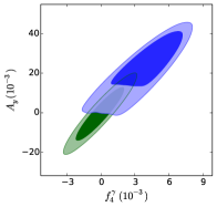
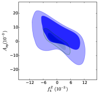
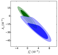
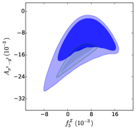
Figure 9: Two-dimensional marginalized contours showing most correlated observable for each parameter of the process $e^{+}e^{-}\rightarrow ZZ$. The upper transparent layer (blue) contours correspond to aTGC, while the lower layer (green) contours correspond to SM. The darker shade shows 68 % contours, while the lighter shade is for 95 % contours

Figure 10: Two-dimensional marginalized contours showing correlation between $A_{zz}$ and $\sigma$ in the $ZZ$ process. The rest of the details are the same as in Fig. 9

We are using a total of six observables, five asymmetries and one cross section for our analysis of two benchmark points; however, we have only four free parameters. This invariably leads to some correlations between the observables apart from the expected correlations between parameters and observables. Figure 9 shows most prominently correlated observable for each of the parameters. The CP nature of observables is reflected in the parameter it is strongly correlated with. We see that $A_{y}$ and $A_{xy}$ are linearly dependent upon both $f_{4}^{\gamma}$ and $f_{4}^{Z}$; however, $A_{y}$ is more sensitive to $f_{4}^{\gamma}$ as shown in Fig. 5 as well. Similarly, for the other asymmetries and parameters one can see a correlation which is consistent with the sensitivity plots in Fig. 5. The strong (and negative) correlation between $A_{zz}$ and $\sigma$ shown in Fig. 10 indicates that any one of them is sufficient for the analysis, in principle. However, in practice the cross section puts a much stronger limit than $A_{zz}$, which explains the much narrower BCI for it as compared to the $1\sigma$ expectation.

Table 7: The list of best-fit points, posterior 68 % and 95 % BCI for the parameters for the process $e^{+}e^{-}\to ZZ$ for both SM and aTGC benchmark points

	SM Benchmark			aTGC Benchmark
$f^{V}_{i}$	68 % BCI	95 % BCI	Best-fit	68 % BCI	95 % BCI	Best-fit
$f_{4}^{\gamma}$	$-0.0001\pm 0.0014$	$-0.0001^{+0.0027}_{-0.0027}$	$-0.0002$	$0.0038^{+0.0026}_{-0.0016}$	$0.0038^{+0.0037}_{-0.0042}$	$0.0044$
$f_{4}^{Z}$	$0.0000\pm 0.0026$	$0.0000^{+0.0049}_{-0.0049}$	$-0.0002$	$0.0010^{+0.0065}_{-0.0055}$	$0.0010^{+0.0098}_{-0.011}$	$0.0050$
$f_{5}^{\gamma}$	$-0.0001\pm 0.0015$	$-0.0001^{+0.0030}_{-0.0029}$	$-0.0002$	$0.0038^{+0.0029}_{-0.0019}$	$0.0038^{+0.0042}_{-0.0047}$	$0.0057$
$f_{5}^{Z}$	$0.0032\pm 0.0028$	$0.0032^{+0.0053}_{-0.0053}$	$0.0000$	$0.0057^{+0.0074}_{-0.0051}$	$0.0057^{+0.010}_{-0.011}$	$0.0037$

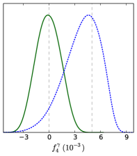
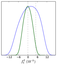
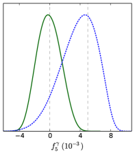
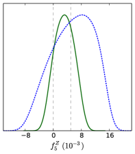
Figure 11: One-dimensional marginalized posterior distribution for the parameters of the process $e^{+}e^{-}\rightarrow ZZ$. Solid (green) lines are for SM and dashed (blue) lines are for aTGC hypothesis. The values of the parameters for the benchmark points are shown by vertical lines for reference

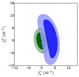
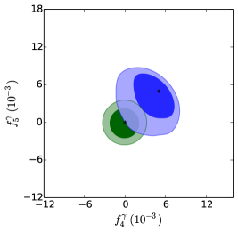
Figure 12: Two-dimensional marginalized contours showing correlations between parameters of the process $e^{+}e^{-}\rightarrow ZZ$. The other details are the same as in Fig. 9.

Finally, we come to the discussion of the parameter estimation. The marginalized one-dimensional posterior distributions for the parameters of $ZZ$ production process are shown in Fig. 11, while the corresponding BCI along with best-fit points are listed in Table 7 for both benchmark points. The vertical lines near zero correspond to the true value of parameters for SM and the other vertical lines correspond to aTGC. The best-fit points are very close to the true values except for $f_{5}^{Z}$ in the aTGC benchmark point due to the multi-valuedness of the cross section. The 95 % BCI of the parameters for two benchmark points overlap and it appears as if they cannot be resolved. To see the resolution better we plot two-dimensional posteriors in Fig. 12, with the benchmark points shown with an asterisk. Again we see that the 95 % contours do overlap as these contours are obtained after marginalizing over non-shown parameters in each panel. Any higher-dimensional representation is not possible on paper, but we have checked three-dimensional scatter plot of points on the Markov chains and conclude that the shape of the good likelihood region is ellipsoidal for the SM point with the true value at its centre. The corresponding three-dimensional shape for the aTGC point is like a part of an ellipsoidal shell. Thus in full four-dimension there will not be any overlap (see Section 5.3) and we can distinguish the two chosen benchmark points as it is quite obvious from the corresponding cross sections. However, left to only the cross section we would have the entire ellipsoidal shell as possible range of parameters for the aTGC case. The presence of asymmetries in our analysis helps narrow down to a part of the ellipsoid and hence aids the parameter estimation for the $ZZ$ production process.

5.2 MCMC analysis for $e^{+}e^{-}\to Z\gamma$

Next we look at the process $e^{+}e^{-}\to Z\gamma$ and $Z\to l^{+}l^{-}$ with $l^{-}=e^{-},\mu^{-}$ in the MadGraph5 simulations. The total cross section for this whole process is given by

$$\sigma=\sigma(e^{-}e^{+}\to Z\gamma)\times Br(Z\to l^{+}l^{-}).$$ (30)

The theoretical values of the cross section and asymmetries (using expression in B) are given in the second column of Tables 8 and 9 for SM and aTGC points, respectively. The tables contain the MadGraph5 simulated data for $L=100$ fb^-1 along with 68 % and 95 % BCI for the observables obtained from the MCMC analysis. For the SM point, Table 8, we notice that the 68 % BCI for all the observables are narrower than the $1\sigma$ range of the psuedo data from MadGraph5. This is again related to the correlations between observables and the fact that the cross section has a lower bound of about 111 fb obtained for $h_{3}^{\gamma}\sim-4.2\times 10^{-3}$ with other parameters close to zero. This lower bound of the cross section leads to narrowing of 68 % BCI for $\sigma$ and hence for other asymmetries too, as observed in the $ZZ$ production process. The 68 % BCI for $A_{x^{2}-y^{2}}$ and $A_{zz}$ are particularly narrow. For $A_{zz}$, this is related to the strong correlation between $(\sigma-A_{zz})$, while for $A_{x^{2}-y^{2}}$ the slower dependence on $h_{3}^{\gamma}$ along with strong dependence of $\sigma$ on $h_{3}^{\gamma}$ is the cause of a narrow 68 % BCI.

Table 8: List of observables shown for the process $e^{+}e^{-}\to Z\gamma$ for the SM point with $\sqrt{\hat{s}}=500$ GeV and $L=100$ fb^-1. The rest of the details are the same as in Table 5

Observables	Theoretical (SM)	MadGraph (SM, prior)	68 % BCI (posterior)	95 % BCI (posterior)
$\sigma$	$112.40$ fb	$112.6\pm 1.06$ fb	$112.64^{+0.64}_{-0.91}$ fb	$112.6^{+1.5}_{-1.4}$ pb
$A_{x}$	$0.00480$	$0.0043\pm 0.0094$	$0.0041\pm 0.0088$	$0.0041^{+0.017}_{-0.018}$
$A_{y}$	$0$	$-0.0011\pm 0.0094$	$-0.0009\pm 0.0088$	$-0.0009\pm 0.017$
$A_{xy}$	$0$	$0.0003\pm 0.0094$	$0.0001\pm 0.0065$	$0.0001\pm 0.012$
$A_{x^{2}-y^{2}}$	$0.00527$	$0.0056\pm 0.0094$	$-0.0001^{+0.0064}_{-0.0034}$	$-0.0001^{+0.0079}_{-0.0096}$
$A_{zz}$	$0.17819$	$0.1781\pm 0.0092$	$0.1771^{+0.0043}_{-0.0031}$	$0.1771^{+0.0066}_{-0.0070}$

Table 9: List of observables shown for the process $e^{+}e^{-}\to Z\gamma$ for the aTGC point with $\sqrt{\hat{s}}=500$ GeV and $L=100$ fb^-1. The rest of the details are the same as in Table 5

Observables	Theoretical (aTGC)	MadGraph (aTGC, prior)	68 % BCI (posterior)	95 % BCI (posterior)
$\sigma$	$122.0$ fb	$122.4\pm 1.11$ fb	$122.3\pm 1.0$ fb	$122.3\pm 2.0$ fb
$A_{x}$	$0.02404$	$0.0252\pm 0.0090$	$0.0263\pm 0.0093$	$0.0263\pm 0.018$
$A_{y}$	$-0.01775$	$-0.0165\pm 0.0090$	$-0.0172\pm 0.0092$	$-0.0172\pm 0.018$
$A_{xy}$	$-0.01350$	$-0.0104\pm 0.0090$	$-0.0109^{+0.0069}_{-0.011}$	$-0.0109^{+0.017}_{-0.015}$
$A_{x^{2}-y^{2}}$	$0.01440$	$0.0133\pm 0.0090$	$0.0121^{+0.0055}_{-0.0010}$	$0.0121^{+0.0068}_{-0.012}$
$A_{zz}$	$0.13612$	$0.1361\pm 0.0089$	$0.1351\pm 0.0041$	$0.1351^{+0.0080}_{-0.0079}$

For the aTGC point, there is enough room for the negative fluctuation in the cross section and hence no narrowing of the 68 % BCI is observed for it; see Table 9. The 68 % BCI for $A_{x}$ and $A_{y}$ are comparable to the corresponding $1\sigma$ intervals, while the 68 % BCI for other three asymmetries are certainly narrower than $1\sigma$ intervals. This narrowing, as discussed earlier, is due to the parametric dependence of the observables and their correlations. Each of the parameters has a strong correlation with one of the asymmetries as shown in Fig. 13. The narrow contours indicate that if one can improve the errors on the asymmetries, it will improve the parameter extraction. The steeper is the slope of the narrow contour, the larger will be its improvement. We note that $A_{x}$ and $A_{y}$ have a steep dependence on the corresponding parameters, thus even small variations in the parameters lead to large variations in the asymmetries. For $A_{xy}$ and $A_{x^{2}-y^{2}}$ the parametric dependence is weaker, leading to their smaller variation with the parameters and hence narrower 68 % BCI.

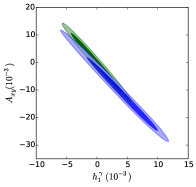
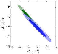
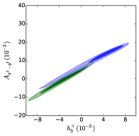
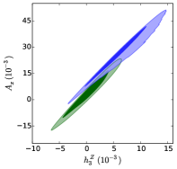
Figure 13: Two-dimensional marginalized contours showing most correlated observables for each parameter of the process $e^{+}e^{-}\rightarrow Z\gamma$ for two benchmark points. The rest of the details are the same as in Fig. 9

Table 10: The list of best-fit points, posterior 68 % and 95 % BCI for the parameters for the process $e^{+}e^{-}\to Z\gamma$ for both benchmark points

	SM Benchmark			aTGC Benchmark
$h^{V}_{i}$	68 % BCI	95 % BCI	Best-fit	68 % BCI	95 % BCI	Best-fit
$h_{1}^{\gamma}$	$-0.0001\pm 0.0026$	$-0.0001^{+0.0048}_{-0.0047}$	$-0.0002$	$0.0039^{+0.0047}_{-0.0031}$	$0.0039^{+0.0068}_{-0.0075}$	$0.0040$
$h_{1}^{Z}$	$0.0003\pm 0.0028$	$0.0003^{+0.0054}_{-0.0054}$	$0.0001$	$0.0050\pm 0.0033$	$0.0050^{+0.0064}_{-0.0063}$	$0.0047$
$h_{3}^{\gamma}$	$-0.0030^{+0.0036}_{-0.0020}$	$-0.0030^{+0.0045}_{-0.0054}$	$0.0002$	$0.00348^{+0.0036}_{-0.00086}$	$0.00348^{+0.0047}_{-0.0076}$	$0.0056$
$h_{3}^{Z}$	$0.0004\pm 0.0028$	$0.0004^{+0.0053}_{-0.0055}$	$-0.0002$	$0.0062^{+0.0030}_{-0.0035}$	$0.0062^{+0.0070}_{-0.0062}$	$0.0052$

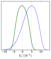
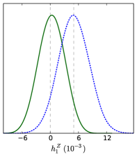
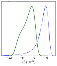
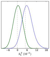
Figure 14: Posterior one-dimensional marginalized distributions for parameters of the process $e^{+}e^{-}\rightarrow Z\gamma$ for SM (green/solid) and aTGC (blue/dashed) points. Vertical lines denote the values of the benchmark points

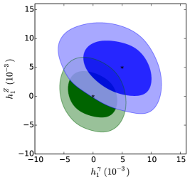
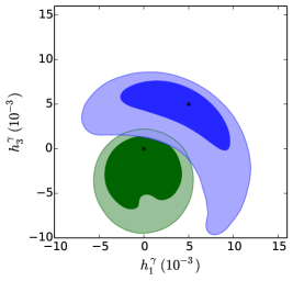
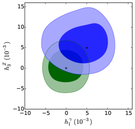
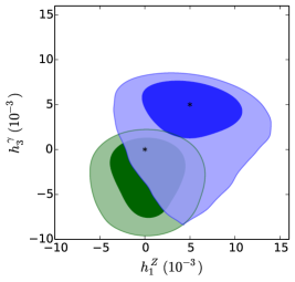
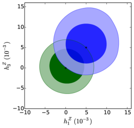
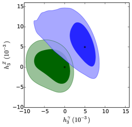
Figure 15: Two-dimensional contours for all pairs of the parameters in the process $e^{+}e^{-}\rightarrow Z\gamma$. The Upper transparent layers (blue) are for aTGC and the lower layers (green) for the SM showing the 68 % BC (dark shades) and 95 % BC (light shades) contours

For the parameter extraction we look at their one-dimensional marginalized posterior distribution function shown in Fig. 14 for the two benchmark points. The best-fit points along with 68 % and 95 % BCI are listed in Table 10. The best-fit points are very close to the true values of the parameters and so are the means of the BCI for all parameters except $h_{3}^{\gamma}$. For it there is a downward movement in the value owing to the multi-valuedness of the cross section. Also, we note that the 95 % BCI for the two benchmark points largely overlap making them seemingly un-distinguishable at the level of one-dimensional BCIs. To highlight the difference between two benchmark points, we look at two-dimensional BC contours as shown in Fig. 15. The 68 % BC contours (dark shades) can be roughly compared with the contours of Fig. 8. The difference is that Fig. 15 has all four parameters varying and all six observables are used simultaneously. The 95 % BC contours for the two benchmark points overlap despite the fact that the cross section can distinguish them very clearly. In full four-dimensional parameter space the two contours do not overlap and in the next section we try to establish this.

5.3 Separability of benchmark points

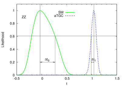
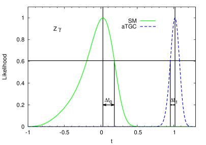
Figure 16: Likelihood ratio for the separability of benchmark points for $ZZ$ (left) and $Z\gamma$ (right) final state: SM pseudo data are in solid (green) and aTGC pseudo data are in dotted (blue) lines

To depict the separability of the two benchmark points pictorially, we vary all four parameters for a chosen process as a linear function of one parameter, $t$, as

$$\vec{f}(t)=(1-t)\ \vec{f}_{\tt SM}+t\ \vec{f}_{\tt aTGC},$$ (31)

such that $\vec{f}(0)=\vec{f}_{\tt SM}$ is the coupling for the SM benchmark point and $\vec{f}(1)=\vec{f}_{\tt aTGC}$ is the coupling for the aTGC point. In Fig. 16 we show the normalized likelihood for the point $\vec{f}(t)$ assuming the SM pseudo data, ${\cal L}(\vec{f}(t)|\mbox{\tt SM})$, in solid/green line and assuming the aTGC pseudo data, ${\cal L}(\vec{f}(t)|\mbox{\tt aTGC})$, in dashed/blue line. The left panel is for the $ZZ$ production process and the right panel is for the $Z\gamma$ process. The horizontal lines correspond to the normalized likelihood being $e^{-\frac{1}{2}}$, while the full vertical lines correspond to the maximum value, which is normalized to $1$. It is clearly visible that the two benchmark points are quite well separated in terms of the likelihood ratios. We have ${\cal L}(\vec{f}_{\tt aTGC}|\mbox{\tt SM})\sim 8.8\times 10^{-19}$ for the $ZZ$ process, and it means that the relative likelihood for the SM pseudo data being generated by the aTGC parameter value is $8.8\times 10^{-19}$, i.e. negligibly small. Comparing the likelihood ratio to $e^{-n^{2}/2}$ we can say that the data is $n\sigma$ away from the model point. In this case, SM pseudo data is $9.1\sigma$ away from the aTGC point for the $ZZ$ process. Similarly we have ${\cal L}(\vec{f}_{\tt SM}|\mbox{\tt aTGC})\sim 1.7\times 10^{-17}$, i.e. the aTGC pseudo data is $8.8\sigma$ away from the SM point for the $ZZ$ process. For the $Z\gamma$ process we have ${\cal L}(\vec{f}_{\tt aTGC}|\mbox{\tt SM})\sim 1.7\times 10^{-24}(10.5\sigma)$ and ${\cal L}(\vec{f}_{\tt SM}|\mbox{\tt aTGC})\sim 1.8\times 10^{-25}(10.7\sigma)$. In all cases the two benchmark points are well separable as clearly seen in Fig. 16.

6 Conclusions

There are angular asymmetries in collider that can be constructed to probe all eight polarization parameters of a massive spin-$1$ particle. Three of them, $A_{y}$, $A_{xy}$, and $A_{yz}$, are CP-odd and can be used to measure CP-violation in the production process. On the other hand $A_{z}$, $A_{xz}$, and $A_{yz}$ are P-odd observables, while $A_{x}$, $A_{x^{2}-y^{2}}$, and $A_{zz}$ are CP- and P-even. The anomalous trilinear gauge coupling in the neutral sector, Eq. (18), is studied using these asymmetries along with the cross section. The one and two parameter sensitivity of these asymmetries, together with cross section, are explored and the one-parameter limit using one observable is listed in Table 4 for an unpolarized $e^{+}e^{-}$ collider. For finding the best and simultaneous limit on anomalous couplings, we have performed a likelihood mapping using the MCMC method and the obtained limits are listed in Tables 7 and 10 for $ZZ$ and $Z\gamma$ processes, respectively. For the $ZZ$ process, the ILC ($\sqrt{\hat{s}}=500$ GeV, ${\cal L}=100$ fb^-1) limits are tighter than the available LHC ($\sqrt{\hat{s}}=7$ TeV, $L=5$ fb^-1) limits Chatrchyan:2012sga , while the ILC limits on the $Z\gamma$ anomalous couplings are slightly weaker than the available LHC ($\sqrt{\hat{s}}=8$ TeV, $L=19.6$ fb^-1) limits Khachatryan:2016yro . The LHC probes the interactions at large energies and transverse momentum, where the sensitivity to the anomalous couplings is enhanced. We perform our analysis at $\sqrt{\hat{s}}=500$ GeV, leading to a weaker, though comparable, limits on the $h_{i}^{V}$ in the $Z\gamma$ process.

With polarized initial beams, the P-odd observables, $A_{z}$, $A_{xz}$, and $A_{yz}$, will be non-vanishing for both process with appropriate kinematical cuts. This gives us three more observables to add in the likelihood analysis, which can lead to better limits. At LHC, one does not have the possibility of initial beam polarization, however, $W^{+}W^{-}$ and $ZW^{\pm}$ processes effectively have initial beam polarization due to chiral couplings of $W^{\pm}$. The study of $W$ and $Z$ processes at LHC and polarized $e^{+}e^{-}$ colliders are underway and will be presented elsewhere.

Acknowledgements: R. R. thanks Department of Science and Technology, Government of India for support through DST-INSPIRE Fellowship for doctoral program, INSPIRE CODE IF140075, 2014.

Appendix A Helicity amplitudes

Vertices in SM are taken as

$$e^{-}e^{+}Z^{\mu}\Rightarrow -i\frac{g_{z}}{2}\gamma^{\mu}\left(C_{L}P_{L}+C_{R}P_{R}\right),$$

$$e^{-}e^{+}\gamma^{\mu}\Rightarrow ig_{e}\gamma^{\mu},$$ (32)

where $C_{L}=-1+2\sin^{2}\theta_{W}$, $C_{R}=2\sin^{2}\theta_{W}$, with $\sin^{2}\theta_{W}=1-\left(\frac{M_{W}}{M_{Z}}\right)^{2}$. Here $\theta_{W}$ is the Weinberg mixing angle. The couplings $g_{e}$, $g_{z}$ are given by

$$g_{e}=\sqrt{4\pi\alpha_{em}}\hskip 28.45274pt\text{and}\hskip 28.45274ptg_{z}=\frac{g_{e}}{\cos\theta_{W}\sin\theta_{W}}.$$ (33)

$P_{L}=\frac{1-\gamma_{5}}{2}$, $P_{R}=\frac{1+\gamma_{5}}{2}$ are the left and right chiral operators. Here $\sin\theta$ and $\cos\theta$ are written as $s_{\theta}$ and $c_{\theta}$ respectively.

A.1 For the process $e^{+}e^{-}\to ZZ$

We define $\beta$ as

$$\beta=\sqrt{1-\frac{4M_{Z}^{2}}{\hat{s}}},$$ (34)

$\sqrt{\hat{s}}$ being the centre-of-mass energy of the colliding beams. We also define $f^{Z}=f_{4}^{Z}+if_{5}^{Z}\beta$, $f^{\gamma}=f_{4}^{\gamma}+if_{5}^{\gamma}\beta$.

$$\mathcal{M}_{\lambda_{e^{-}},\lambda_{e^{+}},\lambda_{z(1)},\lambda_{z(2)}}=\mathcal{M}_{SM}+\mathcal{M}_{aTGC}$$

$$\mathcal{M}_{+,-,+,+} = -\frac{ig_{z}^{2}C_{R}^{2}\left(1-\beta^{2}\right)c_{\theta}s_{\theta}}{1+2\beta^{2}\left(1-2c_{\theta}^{2}\right)+\beta^{4}}$$

$$\mathcal{M}_{+,-,+,0} = -\frac{ig_{z}^{2}C_{R}^{2}\sqrt{1-\beta^{2}}\left(1-2c_{\theta}+\beta^{2}\right)(1+c_{\theta})}{\sqrt{2}\left(1+2\beta^{2}\left(1-2c_{\theta}^{2}\right)+\beta^{4}\right)}$$

$$-\frac{\sqrt{2}\left(1+c_{\theta}\right)g_{e}\beta\left(2g_{e}f^{\gamma}-C_{R}g_{z}f^{Z}\right)}{\left(1-\beta^{2}\right)^{3/2}}$$

$$\mathcal{M}_{+,-,+,-} = \frac{ig_{z}^{2}C_{R}^{2}\left(1+\beta^{2}\right)(1+c_{\theta})s_{\theta}}{1+2\beta^{2}\left(1-2c_{\theta}^{2}\right)+\beta^{4}}$$

$$\mathcal{M}_{+,-,0,+} = \frac{ig_{z}^{2}C_{R}^{2}\sqrt{1-\beta^{2}}\left(1+2c_{\theta}+\beta^{2}\right)(1-c_{\theta})}{\sqrt{2}\left(1+2\beta^{2}\left(1-2c_{\theta}^{2}\right)+\beta^{4}\right)}$$

$$+\frac{\sqrt{2}\left(1-c_{\theta}\right)g_{e}\beta\left(2g_{e}f^{\gamma}-C_{R}g_{z}f^{Z}\right)}{\left(1-\beta^{2}\right)^{3/2}}$$

$$\mathcal{M}_{+,-,0,0} = -\frac{2ig_{z}^{2}C_{R}^{2}\left(1-\beta^{2}\right)c_{\theta}s_{\theta}}{1+2\beta^{2}\left(1-2c_{\theta}^{2}\right)+\beta^{4}}$$

$$\mathcal{M}_{+,-,0,-} = -\frac{ig_{z}^{2}C_{R}^{2}\sqrt{1-\beta^{2}}\left(1-2c_{\theta}+\beta^{2}\right)(1+c_{\theta})}{\sqrt{2}\left(1+2\beta^{2}\left(1-2c_{\theta}^{2}\right)+\beta^{4}\right)}$$

$$+\frac{\sqrt{2}\left(1+c_{\theta}\right)g_{e}\beta\left(2g_{e}{f^{\gamma}}^{\star}-C_{R}g_{z}{f^{Z}}^{\star}\right)}{\left(1-\beta^{2}\right)^{3/2}}$$

$$\mathcal{M}_{+,-,-,+} = -\frac{ig_{z}^{2}C_{R}^{2}\left(1+\beta^{2}\right)(1-c_{\theta})s_{\theta}}{1+2\beta^{2}\left(1-2c_{\theta}^{2}\right)+\beta^{4}}$$

$$\mathcal{M}_{+,-,-,0} = \frac{ig_{z}^{2}C_{R}^{2}\sqrt{1-\beta^{2}}\left(1+2c_{\theta}+\beta^{2}\right)(1-c_{\theta})}{\sqrt{2}\left(1+2\beta^{2}\left(1-2c_{\theta}^{2}\right)+\beta^{4}\right)}$$

$$-\frac{\sqrt{2}\left(1-c_{\theta}\right)g_{e}\beta\left(2g_{e}{f^{\gamma}}^{\star}-C_{R}g_{z}{f^{Z}}^{\star}\right)}{\left(1-\beta^{2}\right)^{3/2}}$$

$$\mathcal{M}_{+,-,-,-} = -\frac{ig_{z}^{2}C_{R}^{2}\left(1-\beta^{2}\right)c_{\theta}s_{\theta}}{1+2\beta^{2}\left(1-2c_{\theta}^{2}\right)+\beta^{4}}$$

$$\mathcal{M}_{-,+,+,+} = -\frac{ig_{z}^{2}C_{L}^{2}\left(1-\beta^{2}\right)c_{\theta}s_{\theta}}{1+2\beta^{2}\left(1-2c_{\theta}^{2}\right)+\beta^{4}}$$

$$\mathcal{M}_{-,+,+,0} = -\frac{ig_{z}^{2}C_{L}^{2}\sqrt{1-\beta^{2}}\left(1+2c_{\theta}+\beta^{2}\right)(1-c_{\theta})}{\sqrt{2}\left(1+2\beta^{2}\left(1-2c_{\theta}^{2}\right)+\beta^{4}\right)}$$

$$+\frac{\sqrt{2}\left(1-c_{\theta}\right)g_{e}\beta\left(2g_{e}f^{\gamma}-C_{L}g_{z}f^{Z}\right)}{\left(1-\beta^{2}\right)^{3/2}}$$

$$\mathcal{M}_{-,+,+,-} = \frac{ig_{z}^{2}C_{L}^{2}\left(1+\beta^{2}\right)(1-c_{\theta})s_{\theta}}{1+2\beta^{2}\left(1-2c_{\theta}^{2}\right)+\beta^{4}}$$

$$\mathcal{M}_{-,+,0,+} = \frac{ig_{z}^{2}C_{L}^{2}\sqrt{1-\beta^{2}}\left(1-2c_{\theta}+\beta^{2}\right)(1+c_{\theta})}{\sqrt{2}\left(1+2\beta^{2}\left(1-2c_{\theta}^{2}\right)+\beta^{4}\right)}$$

$$-\frac{\sqrt{2}\left(1+c_{\theta}\right)g_{e}\beta\left(2g_{e}f^{\gamma}-C_{L}g_{z}f^{Z}\right)}{\left(1-\beta^{2}\right)^{3/2}}$$

$$\mathcal{M}_{-,+,0,0} = -\frac{2ig_{z}^{2}C_{L}^{2}\left(1-\beta^{2}\right)c_{\theta}s_{\theta}}{1+2\beta^{2}\left(1-2c_{\theta}^{2}\right)+\beta^{4}}$$

$$\mathcal{M}_{-,+,0,-} = -\frac{ig_{z}^{2}C_{L}^{2}\sqrt{1-\beta^{2}}\left(1+2c_{\theta}+\beta^{2}\right)(1-c_{\theta})}{\sqrt{2}\left(1+2\beta^{2}\left(1-2c_{\theta}^{2}\right)+\beta^{4}\right)}$$

$$-\frac{\sqrt{2}\left(1-c_{\theta}\right)g_{e}\beta\left(2g_{e}{f^{\gamma}}^{\star}-C_{L}g_{z}{f^{Z}}^{\star}\right)}{\left(1-\beta^{2}\right)^{3/2}}$$

$$\mathcal{M}_{-,+,-,+} = \frac{ig_{z}^{2}C_{L}^{2}\left(1+\beta^{2}\right)(1+c_{\theta})s_{\theta}}{1+2\beta^{2}\left(1-2c_{\theta}^{2}\right)+\beta^{4}}$$

$$\mathcal{M}_{-,+,-,0} = \frac{ig_{z}^{2}C_{L}^{2}\sqrt{1-\beta^{2}}\left(1-2c_{\theta}+\beta^{2}\right)(1+c_{\theta})}{\sqrt{2}\left(1+2\beta^{2}\left(1-2c_{\theta}^{2}\right)+\beta^{4}\right)}$$

$$+\frac{\sqrt{2}\left(1+c_{\theta}\right)g_{e}\beta\left(2g_{e}{f^{\gamma}}^{\star}-C_{L}g_{z}{f^{Z}}^{\star}\right)}{\left(1-\beta^{2}\right)^{3/2}}$$

$$\mathcal{M}_{-,+,-,-} = -\frac{ig_{z}^{2}C_{L}^{2}\left(1-\beta^{2}\right)c_{\theta}s_{\theta}}{1+2\beta^{2}\left(1-2c_{\theta}^{2}\right)+\beta^{4}}$$ (35)

A.2 For the process $e^{+}e^{-}\to Z\gamma$

In this process $\beta$ is given by

$$\beta=1-\frac{M_{Z}^{2}}{\hat{s}}.$$ (36)

We define $h^{\gamma}=h_{1}^{\gamma}+ih_{3}^{\gamma}$ and $h^{Z}=h_{1}^{Z}+ih_{3}^{Z}$.

$$\mathcal{M}_{\lambda_{e^{-}},\lambda_{e^{+}},\lambda_{z},\lambda_{\gamma}} = \mathcal{M}_{SM}+\mathcal{M}_{aTGC}$$

$$\mathcal{M}_{+,-,+,+} = \frac{-ig_{e}g_{z}C_{R}s_{\theta}(1-\beta)}{\beta(1-c_{\theta})}$$

$$-\frac{g_{e}\left(2g_{e}h^{\gamma}-C_{R}g_{z}h^{Z}\right)s_{\theta}\beta}{4(1-\beta)}$$

$$\mathcal{M}_{+,-,+,-} = \frac{ig_{e}g_{z}C_{R}s_{\theta}}{\beta(1-c_{\theta})}$$

$$\mathcal{M}_{+,-,0,+} = \frac{i\sqrt{2}g_{e}g_{z}C_{R}\sqrt{1-\beta}}{\beta}$$

$$+\frac{\left(1-c_{\theta}\right)g_{e}\left(2g_{e}h^{\gamma}-C_{R}g_{z}h^{Z}\right)\beta}{4\sqrt{2}(1-\beta)^{3/2}}$$

$$\mathcal{M}_{+,-,0,-} = \frac{-i\sqrt{2}g_{e}g_{z}C_{R}\sqrt{1-\beta}}{\beta}$$

$$+\frac{\left(1+c_{\theta}\right)g_{e}\left(2g_{e}{h^{\gamma}}^{\star}-C_{R}g_{z}{h^{Z}}^{\star}\right)\beta}{4\sqrt{2}(1-\beta)^{3/2}}$$

$$\mathcal{M}_{+,-,-,+} = \frac{-ig_{e}g_{z}C_{R}s_{\theta}}{\beta(1+c_{\theta})}$$

$$\mathcal{M}_{+,-,-,-} = \frac{ig_{e}g_{z}(1-\beta)s_{\theta}}{\beta(1+c_{\theta})}$$

$$-\frac{g_{e}\left(2g_{e}{h^{\gamma}}^{\star}-C_{R}g_{z}{h^{Z}}^{\star}\right)s_{\theta}\beta}{4(1-\beta)}$$

$$\mathcal{M}_{-,+,+,+} = \frac{ig_{e}g_{z}C_{L}s_{\theta}(1-\beta)}{\beta({1+\text{c}_{\theta}})}$$

$$-\frac{g_{e}\left(2g_{e}h^{\gamma}-C_{L}g_{z}h^{Z}\right)s_{\theta}\beta}{4(1-\beta)}$$

$$\mathcal{M}_{-,+,+,-} = \frac{-ig_{e}g_{z}C_{L}s_{\theta}}{\beta(1+c_{\theta})}$$

$$\mathcal{M}_{-,+,0,+} = \frac{i\sqrt{2}g_{e}g_{z}C_{L}\sqrt{1-\beta}}{\beta}$$

$$-\frac{\left(1+c_{\theta}\right)g_{e}\left(2g_{e}h^{\gamma}-C_{L}g_{z}h^{Z}\right)\beta}{4\sqrt{2}(1-\beta)^{3/2}}$$

$$\mathcal{M}_{-,+,0,-} = \frac{-i\sqrt{2}g_{e}g_{z}C_{L}\sqrt{1-\beta}}{\beta}$$

$$-\frac{\left(1-c_{\theta}\right)g_{e}\left(2g_{e}{h^{\gamma}}^{\star}-C_{L}g_{z}{h^{Z}}^{\star}\right)\beta}{4\sqrt{2}(1-\beta)^{3/2}}$$

$$\mathcal{M}_{-,+,-,+} = \frac{ig_{e}g_{z}C_{L}s_{\theta}}{\beta(1-c_{\theta})}$$

$$\mathcal{M}_{-,+,-,-} = \frac{-ig_{e}g_{z}C_{L}(1-\beta)s_{\theta}}{\beta(1-c_{\theta})}$$ (37)

$$-\frac{g_{e}\left(2g_{e}{h^{\gamma}}^{\star}-C_{L}g_{z}{h^{Z}}^{\star}\right)s_{\theta}\beta}{4(1-\beta)}$$

Appendix B Polarization observables

B.1 For the process $e^{+}e^{-}\to ZZ$

$$\sigma(e^{+}e^{-}\to ZZ)=\frac{1}{2}\dfrac{1}{32\pi\beta\hat{s}}\ \tilde{\sigma}_{ZZ}$$ (38)

$$\tilde{\sigma}_{ZZ}=\frac{1}{2}g_{Z}^{4}\left(C_{L}^{4}+C_{R}^{4}\right)\left(\frac{\left(5-2\beta^{2}+\beta^{4}\right)\log\left(\frac{1+\beta}{1-\beta}\right)}{2\left(\beta+\beta^{3}\right)}-1\right)$$

$$+g_{Z}^{3}g_{e}\left(C_{L}^{3}-C_{R}^{3}\right)f_{5}^{Z}\frac{\left(3-\beta^{2}\right)\left(2\beta+\left(1+\beta^{2}\right)\log\left(\frac{1+\beta}{1-\beta}\right)\right)}{2\beta\left(1-\beta^{2}\right)}$$

$$-g_{Z}^{2}g_{e}^{2}\left(C_{L}^{2}-C_{R}^{2}\right)f_{5}^{\gamma}\frac{\left(3-\beta^{2}\right)\left(2\beta-\left(1+\beta^{2}\right)\log\left(\frac{1+\beta}{1-\beta}\right)\right)}{\beta\left(1-\beta^{2}\right)}$$

$$+16g_{Z}^{2}g_{e}^{2}\left(C_{L}^{2}+C_{R}^{2}\right)\frac{\beta^{2}\left((f_{4}^{Z})^{2}+(f_{5}^{Z})^{2}\beta^{2}\right)}{3\left(1-\beta^{2}\right)^{3}}$$

$$-64g_{Z}g_{e}^{3}\left(C_{L}+C_{R}\right)\frac{\beta^{2}\left(f_{4}^{\gamma}f_{4}^{Z}+f_{5}^{\gamma}f_{5}^{Z}\beta^{2}\right)}{3\left(1-\beta^{2}\right)^{3}}$$

$$+128g_{e}^{4}\frac{\beta^{2}\left((f_{4}^{\gamma})^{2}+(f_{5}^{\gamma})^{2}\beta^{2}\right)}{3\left(1-\beta^{2}\right)^{3}}$$ (39)

$$\tilde{\sigma}_{ZZ}\times P_{x}= g_{Z}^{4}\left(C_{L}^{4}-C_{R}^{4}\right)\frac{\pi(1-\beta^{2})^{3/2}}{4(1+\beta^{2})}$$ (40)

$$+ g_{z}^{3}g_{e}\left(C_{L}^{3}+C_{R}^{3}\right)\frac{f_{5}^{Z}\pi\beta^{2}(1+2\beta^{2})}{4(1-\beta^{2})^{3/2}}$$

$$- g_{z}^{2}g_{e}^{2}\left(C_{L}^{2}+C_{R}^{2}\right)\frac{f_{5}^{\gamma}\pi\beta^{2}(1+2\beta^{2})}{2(1-\beta^{2})^{3/2}}$$

$$\tilde{\sigma}_{ZZ}\times P_{y}= - g_{z}^{3}g_{e}\left(C_{L}^{3}+C_{R}^{3}\right)\frac{f_{4}^{Z}\pi\beta(2+\beta^{2})}{4(1-\beta^{2})^{3/2}}$$ (41)

$$+ g_{z}^{2}g_{e}^{2}\left(C_{L}^{2}+C_{R}^{2}\right)\frac{f_{4}^{\gamma}\pi\beta(2+\beta^{2})}{2(1-\beta^{2})^{3/2}}$$

$$\tilde{\sigma}_{ZZ}\times T_{xy}=g_{Z}^{3}g_{e}\left(C_{L}^{3}-C_{R}^{3}\right)\frac{\sqrt{3}}{8}f_{4}^{Z}f_{xy}(\beta)$$

$$-g_{Z}^{2}g_{e}^{2}\left(C_{L}^{2}-C_{R}^{2}\right)\frac{\sqrt{3}}{4}f_{4}^{\gamma}f_{xy}(\beta)$$

$$+g_{Z}^{2}g_{e}^{2}\left(C_{L}^{2}+C_{R}^{2}\right)\frac{4}{\sqrt{3}}\frac{f_{4}^{Z}f_{5}^{Z}\beta^{3}}{\left(1-\beta^{2}\right)^{3}}$$

$$+g_{Z}g_{e}^{3}\left(C_{L}+C_{R}\right)\frac{8}{\sqrt{3}}\frac{\left(f_{4}^{Z}f_{5}^{\gamma}+f_{4}^{\gamma}f_{5}^{Z}\right)\beta^{3}}{\left(1-\beta^{2}\right)^{3}}$$

$$+g_{e}^{4}\frac{32f_{4}^{\gamma}f_{5}^{\gamma}\beta^{3}}{\sqrt{3}\left(1-\beta^{2}\right)^{3}},$$

$$f_{xy}(\beta)=\frac{\left(2\left(\beta+\beta^{3}\right)-\left(1-\beta^{2}\right)^{2}\log\left(\frac{1+\beta}{1-\beta}\right)\right)}{\beta^{2}\left(1-\beta^{2}\right)}$$ (42)

$$\tilde{\sigma}_{ZZ}\times(T_{xx}-T_{yy})=$$

$$g_{Z}^{4}\left(C_{L}^{4}+C_{R}^{4}\right)\sqrt{\frac{3}{2}}\frac{\left(1-\beta^{2}\right)\left(2\beta-\left(1+\beta^{2}\right)\log\left(\frac{1+\beta}{1-\beta}\right)\right)}{8\beta^{3}}$$

$$-\bigg{(}g_{Z}^{3}g_{e}\left(C_{L}^{3}-C_{R}^{3}\right)f_{5}^{Z}+g_{Z}^{2}g_{e}^{2}\left(C_{L}^{2}-C_{R}^{2}\right)2f_{5}^{\gamma}\bigg{)}f_{x^{2}-y^{2}}(\beta)$$

$$+g_{Z}^{2}g_{e}^{2}\left(C_{L}^{2}+C_{R}^{2}\right)2\sqrt{\frac{2}{3}}\frac{\beta^{2}\left((f_{4}^{Z})^{2}-(f_{5}^{Z})^{2}\beta^{2}\right)}{\left(1-\beta^{2}\right)^{3}}$$

$$-g_{Z}g_{e}^{3}\left(C_{L}+C_{R}\right)8\sqrt{\frac{2}{3}}\frac{\beta^{2}\left(f_{4}^{\gamma}f_{4}^{Z}-f_{5}^{\gamma}f_{5}^{Z}\beta^{2}\right)}{\left(1-\beta^{2}\right)^{3}}$$

$$+g_{e}^{4}16\sqrt{\frac{2}{3}}\frac{\beta^{2}\left((f_{4}^{\gamma})^{2}-(f_{5}^{\gamma})^{2}\beta^{2}\right)}{\left(1-\beta^{2}\right)^{3}},$$

$$f_{x^{2}-y^{2}}(\beta)=\sqrt{\frac{3}{2}}\frac{\left(2\left(\beta+\beta^{3}\right)-\left(1-\beta^{2}\right)^{2}\log\left(\frac{1+\beta}{1-\beta}\right)\right)}{4\beta\left(1-\beta^{2}\right)}$$

$$\tilde{\sigma}_{ZZ}\times T_{ZZ}=g_{Z}^{4}\left(C_{L}^{4}+C_{R}^{4}\right)\frac{f_{zz}(\beta)}{8\sqrt{6}\beta^{3}\left(1+\beta^{2}\right)}$$ (44)

$$+g_{Z}^{3}g_{e}\left(C_{L}^{3}-C_{R}^{3}\right)f_{5}^{Z}\frac{f_{zz}(\beta)}{4\sqrt{6}\beta\left(1-\beta^{2}\right)}$$

$$- g_{Z}^{2}g_{e}^{2}\left(C_{L}^{2}-C_{R}^{2}\right)f_{5}^{\gamma}\frac{f_{zz}(\beta)}{2\sqrt{6}\beta\left(1-\beta^{2}\right)}$$

$$-g_{Z}^{2}g_{e}^{2}\left(C_{L}^{2}+C_{R}^{2}\right)\frac{4}{3}\sqrt{\frac{2}{3}}\frac{\beta^{2}\left((f_{4}^{Z})^{2}+(f_{5}^{Z})^{2}\beta^{2}\right)}{\left(1-\beta^{2}\right)^{3}}$$

$$+g_{Z}g_{e}^{3}\left(C_{L}+C_{R}\right)\frac{16}{3}\sqrt{\frac{2}{3}}\frac{\beta^{2}\left(f_{4}^{\gamma}f_{4}^{Z}+f_{5}^{\gamma}f_{5}^{Z}\beta^{2}\right)}{\left(1-\beta^{2}\right)^{3}}$$

$$-g_{e}^{4}\frac{32}{3}\sqrt{\frac{2}{3}}\frac{\beta^{2}\left((f_{4}^{\gamma})^{2}+(f_{5}^{\gamma})^{2}\beta^{2}\right)}{\left(1-\beta^{2}\right)^{3}},$$

$$f_{zz}(\beta)=\bigg{(}\left(3+\beta^{2}+5\beta^{4}-\beta^{6}\right)\log\left(\frac{1+\beta}{1-\beta}\right)\bigg{.}$$

$$\hskip 42.67912pt\bigg{.}-2\beta\left(3-\beta^{2}\right)\left(1+\beta^{2}\right)\bigg{)}$$

B.2 For the process $e^{+}e^{-}\to Z\gamma$

$$\sigma(e^{+}e^{-}\to Z\gamma)=\dfrac{1}{32\pi\beta\hat{s}}\ \tilde{\sigma}_{Z\gamma},\ \ \ c_{\theta}\in[-c_{\theta_{0}},c_{\theta_{0}}]$$ (45)

$$\tilde{\sigma}_{Z\gamma}=-g_{e}^{2}g_{Z}^{2}\left(C_{L}^{2}+C_{R}^{2}\right)\frac{1}{\beta^{2}}\bigg{(}c_{\theta_{0}}\beta^{2}\bigg{.}$$ (46)

$$-\bigg{.}2\left(2-2\beta+\beta^{2}\right)\tanh^{-1}(c_{\theta_{0}})\bigg{)}$$

$$+g_{e}^{2}g_{Z}^{2}\left(C_{L}^{2}-C_{R}^{2}\right)\frac{c_{\theta_{0}}h_{3}^{Z}(2-\beta)}{2(1-\beta)}$$

$$-g_{e}^{3}g_{Z}\left(C_{L}-C_{R}\right)\frac{c_{\theta_{0}}h_{3}^{\gamma}(2-\beta)}{(1-\beta)}$$

$$+g_{e}^{2}g_{Z}^{2}\left(C_{L}^{2}+C_{R}^{2}\right)c_{\theta_{0}}\left((h_{1}^{Z})^{2}+(h_{3}^{Z})^{2}\right)h_{\sigma}(\beta)$$

$$- g_{e}^{3}g_{Z}\left(C_{L}+C_{R}\right)c_{\theta_{0}}\left(h_{1}^{\gamma}h_{1}^{Z}+h_{3}^{\gamma}h_{3}^{Z}\right)4h_{\sigma}(\beta)$$

$$+g_{e}^{4}c_{\theta_{0}}\left((h_{1}^{\gamma})^{2}+(h_{3}^{\gamma})^{2}\right)8h_{\sigma}(\beta),$$

$$h_{\sigma}(\beta)=\frac{\beta^{2}\left(9-6\beta-c_{\theta_{0}}^{2}(1-2\beta)\right)}{96(1-\beta)^{3}}$$

$$\tilde{\sigma}_{Z\gamma}\times P_{x}=$$

$$g_{e}^{2}g_{Z}^{2}\left(C_{L}^{2}-C_{R}^{2}\right)2\frac{\sqrt{1-\beta}}{\beta^{2}}(2-\beta)\sinh^{-1}(c_{\theta_{0}})$$

$$+g_{e}^{2}g_{Z}^{2}\left(C_{L}^{2}+C_{R}^{2}\right)h_{3}^{Z}h_{x}^{1}(\beta)-g_{e}^{3}g_{Z}\left(C_{L}+C_{R}\right)h_{3}^{\gamma}2h_{x}^{1}(\beta)$$

$$+g_{e}^{2}g_{Z}^{2}\left(C_{L}^{2}-C_{R}^{2}\right)\left((h_{1}^{Z})^{2}+(h_{3}^{Z})^{2}\right)h_{x}^{2}(\beta)$$

$$-g_{e}^{3}g_{Z}\left(C_{L}-C_{R}\right)\left(h_{1}^{\gamma}h_{1}^{Z}+h_{3}^{\gamma}h_{3}^{Z}\right)4h_{x}^{2}(\beta),$$

$$h_{x}^{1}(\beta)=\frac{\left(c_{\theta_{0}}s_{\theta_{0}}(2-3\beta)-3(2-\beta)\sinh^{-1}(c_{\theta_{0}})\right)}{8(1-\beta)^{3/2}},$$

$$h_{x}^{2}(\beta)=\frac{\beta^{2}\left(c_{\theta_{0}}s_{\theta_{0}}+\sinh^{-1}(c_{\theta_{0}})\right)}{32(1-\beta)^{5/2}}$$ (47)

$$\tilde{\sigma}_{Z\gamma}\times P_{y}=$$

$$g_{e}^{2}g_{Z}^{2}\left(C_{L}^{2}+C_{R}^{2}\right)\frac{h_{1}^{Z}\bigg{(}c_{\theta_{0}}s_{\theta_{0}}\beta-(4-\beta)\sin^{-1}(c_{\theta_{0}})\bigg{)}}{8(1-\beta)^{3/2}}$$

$$-g_{e}^{3}g_{Z}\left(C_{L}+C_{R}\right)\frac{h_{1}^{\gamma}\bigg{(}c_{\theta_{0}}s_{\theta_{0}}\beta-(4-\beta)\sin^{-1}(c_{\theta_{0}})\bigg{)}}{4(1-\beta)^{3/2}}$$ (48)

$$\tilde{\sigma}_{Z\gamma}\times T_{xy} = g_{e}^{3}g_{Z}\left(C_{L}-C_{R}\right)\frac{\sqrt{3}}{2}\frac{h_{1}^{\gamma}c_{\theta_{0}}}{2(1-\beta)}$$ (49)

$$- g_{e}^{2}g_{Z}^{2}\left(C_{L}^{2}-C_{R}^{2}\right)\frac{\sqrt{3}}{4}\frac{h_{1}^{Z}c_{\theta_{0}}}{4(1-\beta)}$$

$$\tilde{\sigma}_{Z\gamma}\times(T_{xx}-T_{yy})= g_{e}^{2}g_{Z}^{2}\left(C_{L}^{2}+C_{R}^{2}\right)\frac{\sqrt{6}c_{\theta_{0}}(1-\beta)}{\beta^{2}}$$ (50)

$$- g_{e}^{3}g_{Z}\left(C_{L}-C_{R}\right)\sqrt{\frac{3}{2}}\frac{h_{3}^{\gamma}c_{\theta_{0}}}{(1-\beta)}$$

$$\tilde{\sigma}_{Z\gamma}\times T_{zz}=-g_{e}^{2}g_{Z}^{2}\left(C_{L}^{2}+C_{R}^{2}\right)\frac{1}{\sqrt{6}\beta^{2}}\bigg{(}c_{\theta_{0}}\left(6-6\beta+\beta^{2}\right)\bigg{.}$$

$$\bigg{.}-2\left(2-2\beta+\beta^{2}\right)\tanh^{-1}(c_{\theta_{0}})\bigg{)}$$

$$-g_{e}^{2}g_{Z}^{2}\left(C_{L}^{2}-C_{R}^{2}\right)\frac{c_{\theta_{0}}h_{3}^{Z}(1+\beta)}{2\sqrt{6}(1-\beta)}$$

$$+g_{e}^{3}g_{Z}\left(C_{L}-C_{R}\right)\frac{c_{\theta_{0}}h_{3}^{\gamma}(1+\beta)}{\sqrt{6}(1-\beta)}$$

$$-g_{e}^{2}g_{Z}^{2}\left(C_{L}^{2}+C_{R}^{2}\right)c_{\theta_{0}}\left((h_{1}^{Z})^{2}+(h_{3}^{Z})^{2}\right)h_{zz}(\beta)$$

$$+g_{e}^{3}g_{Z}\left(C_{L}+C_{R}\right)c_{\theta_{0}}\left(h_{1}^{\gamma}h_{1}^{Z}+h_{3}^{\gamma}h_{3}^{Z}\right)4h_{zz}(\beta)$$

$$-g_{e}^{4}c_{\theta_{0}}\left((h_{1}^{\gamma})^{2}+(h_{3}^{\gamma})^{2}\right)8h_{zz}(\beta),$$

$$h_{zz}(\beta)=\frac{\left(c_{\theta_{0}}^{2}(2-\beta)+3\beta\right)\beta^{2}}{48\sqrt{6}(1-\beta)^{3}}$$ (51)

References

- (1) CMS Collaboration, S. Chatrchyan et al., Observation of a new boson at a mass of 125 GeV with the CMS experiment at the LHC, Phys. Lett. B716 (2012) 30–61, arXiv:1207.7235 [hep-ex].
- (2) T. Behnke, J. E. Brau, B. Foster, J. Fuster, M. Harrison, J. M. Paterson, M. Peskin, M. Stanitzki, N. Walker, and H. Yamamoto, The International Linear Collider Technical Design Report - Volume 1: Executive Summary, arXiv:1306.6327 [physics.acc-ph].
- (3) H. Baer, T. Barklow, K. Fujii, Y. Gao, A. Hoang, S. Kanemura, J. List, H. E. Logan, A. Nomerotski, M. Perelstein, et al., The International Linear Collider Technical Design Report - Volume 2: Physics, arXiv:1306.6352 [hep-ph].
- (4) K. J. F. Gaemers and G. J. Gounaris, Polarization Amplitudes for and , Z. Phys. C1 (1979) 259.
- (5) F. M. Renard, Tests of Neutral Gauge Boson Selfcouplings With , Nucl. Phys. B196 (1982) 93–108.
- (6) K. Hagiwara, R. D. Peccei, D. Zeppenfeld, and K. Hikasa, Probing the Weak Boson Sector in , Nucl. Phys. B282 (1987) 253–307.
- (7) W. Buchmuller and D. Wyler, Effective Lagrangian Analysis of New Interactions and Flavor Conservation, Nucl. Phys. B268 (1986) 621–653.
- (8) F. Larios, M. A. Perez, G. Tavares-Velasco, and J. J. Toscano, Trilinear neutral gauge boson couplings in effective theories, Phys. Rev. D63 (2001) 113014, arXiv:hep-ph/0012180 [hep-ph].
- (9) O. Cata, Revisiting and production with effective field theories, arXiv:1304.1008 [hep-ph].
- (10) C. Degrande, A basis of dimension-eight operators for anomalous neutral triple gauge boson interactions, JHEP 02 (2014) 101, arXiv:1308.6323 [hep-ph].
- (11) H. Czyz, K. Kolodziej, and M. Zralek, Composite Boson and CP Violation in the Process , Z. Phys. C43 (1989) 97.
- (12) F. Boudjema, Proc. of the Workshop on Collisions at 500GeV: The Physics Potential, edited by P.M. Zerwas, DESY 92-123B (1992) 757.
- (13) U. Baur and E. L. Berger, Probing the weak boson sector in production at hadron colliders, Phys. Rev. D47 (1993) 4889–4904.
- (14) D. Choudhury and S. D. Rindani, Test of CP violating neutral gauge boson vertices in , Phys. Lett. B335 (1994) 198–204, arXiv:hep-ph/9405242 [hep-ph].
- (15) S. Y. Choi, Probing the weak boson sector in , Z. Phys. C68 (1995) 163–172, arXiv:hep-ph/9412300 [hep-ph].
- (16) H. Aihara et al., Anomalous gauge boson interactions, arXiv:hep-ph/9503425 [hep-ph].
- (17) J. Ellison and J. Wudka, Study of trilinear gauge boson couplings at the Tevatron collider, Ann. Rev. Nucl. Part. Sci. 48 (1998) 33–80, arXiv:hep-ph/9804322 [hep-ph].
- (18) G. J. Gounaris, J. Layssac, and F. M. Renard, Signatures of the anomalous and production at the lepton and hadron colliders, Phys. Rev. D61 (2000) 073013, arXiv:hep-ph/9910395 [hep-ph].
- (19) G. J. Gounaris, J. Layssac, and F. M. Renard, Off-shell structure of the anomalous and selfcouplings, Phys. Rev. D65 (2002) 017302, arXiv:hep-ph/0005269 [hep-ph]. [Phys. Rev.D62,073012(2000)].
- (20) U. Baur and D. L. Rainwater, Probing neutral gauge boson selfinteractions in production at hadron colliders, Phys. Rev. D62 (2000) 113011, arXiv:hep-ph/0008063 [hep-ph].
- (21) T. G. Rizzo, Polarization asymmetries in gamma e collisions and triple gauge boson couplings revisited, in Physics and experiments with future linear e+ e- colliders. Proceedings, 4th Workshop, LCWS’99, Sitges, Spain, April 28-May 5, 1999. Vol. 1: Physics at linear colliders, pp. 529–533. 1999. arXiv:hep-ph/9907395 [hep-ph]. http://www-public.slac.stanford.edu/sciDoc/docMeta.aspx?slacPubNumber=SLAC-PUB-8192.
- (22) S. Atag and I. Sahin, ZZ gamma and Z gamma gamma couplings in gamma e collision with polarized beams, Phys. Rev. D68 (2003) 093014, arXiv:hep-ph/0310047 [hep-ph].
- (23) B. Ananthanarayan, S. D. Rindani, R. K. Singh, and A. Bartl, Transverse beam polarization and CP-violating triple-gauge-boson couplings in , Phys. Lett. B593 (2004) 95–104, arXiv:hep-ph/0404106 [hep-ph]. [Erratum: Phys. Lett.B608,274(2005)].
- (24) B. Ananthanarayan, S. K. Garg, M. Patra, and S. D. Rindani, Isolating CP-violating ZZ coupling in Z with transverse beam polarizations, Phys. Rev. D85 (2012) 034006, arXiv:1104.3645 [hep-ph].
- (25) B. Ananthanarayan, J. Lahiri, M. Patra, and S. D. Rindani, New physics in at the ILC with polarized beams: explorations beyond conventional anomalous triple gauge boson couplings, JHEP 08 (2014) 124, arXiv:1404.4845 [hep-ph].
- (26) P. Poulose and S. D. Rindani, CP violating and top quark electric dipole couplings in , Phys. Lett. B452 (1999) 347–354, arXiv:hep-ph/9809203 [hep-ph].
- (27) G. J. Gounaris, J. Layssac, and F. M. Renard, New and standard physics contributions to anomalous Z and gamma selfcouplings, Phys. Rev. D62 (2000) 073013, arXiv:hep-ph/0003143 [hep-ph].
- (28) D. Choudhury, S. Dutta, S. Rakshit, and S. Rindani, Trilinear neutral gauge boson couplings, Int. J. Mod. Phys. A16 (2001) 4891–4910, arXiv:hep-ph/0011205 [hep-ph].
- (29) S. Dutta, A. Goyal, and Mamta, New Physics Contribution to Neutral Trilinear Gauge Boson Couplings, Eur. Phys. J. C63 (2009) 305–315, arXiv:0901.0260 [hep-ph].
- (30) N. G. Deshpande and X.-G. He, Triple neutral gauge boson couplings in noncommutative standard model, Phys. Lett. B533 (2002) 116–120, arXiv:hep-ph/0112320 [hep-ph].
- (31) N. G. Deshpande and S. K. Garg, Anomalous triple gauge boson couplings in for noncommutative standard model, Phys. Lett. B708 (2012) 150–156, arXiv:1111.5173 [hep-ph].
- (32) L3 Collaboration, M. Acciarri et al., Search for anomalous and couplings in the process at LEP, Phys. Lett. B489 (2000) 55–64, arXiv:hep-ex/0005024 [hep-ex].
- (33) OPAL Collaboration, G. Abbiendi et al., Search for trilinear neutral gauge boson couplings in gamma production at = 189-GeV at LEP, Eur. Phys. J. C17 (2000) 553–566, arXiv:hep-ex/0007016 [hep-ex].
- (34) OPAL Collaboration, G. Abbiendi et al., Study of Z pair production and anomalous couplings in e+ e- collisions at between 190-GeV and 209-GeV, Eur. Phys. J. C32 (2003) 303–322, arXiv:hep-ex/0310013 [hep-ex].
- (35) L3 Collaboration, P. Achard et al., Study of the process at LEP and limits on triple neutral-gauge-boson couplings, Phys. Lett. B597 (2004) 119–130, arXiv:hep-ex/0407012 [hep-ex].
- (36) DELPHI Collaboration, J. Abdallah et al., Study of triple-gauge-boson couplings ZZZ, ZZgamma and Zgamma gamma LEP, Eur. Phys. J. C51 (2007) 525–542, arXiv:0706.2741 [hep-ex].
- (37) D0 Collaboration, V. M. Abazov et al., Search for and production in collisions at = 1.96 TeV and limits on anomalous and couplings, Phys. Rev. Lett. 100 (2008) 131801, arXiv:0712.0599 [hep-ex].
- (38) CDF Collaboration, T. Aaltonen et al., Limits on Anomalous Trilinear Gauge Couplings in Events from Collisions at TeV, Phys. Rev. Lett. 107 (2011) 051802, arXiv:1103.2990 [hep-ex].
- (39) D0 Collaboration, V. M. Abazov et al., production and limits on anomalous and couplings in collisions at TeV, Phys. Rev. D85 (2012) 052001, arXiv:1111.3684 [hep-ex].
- (40) CMS Collaboration, S. Chatrchyan et al., Measurement of the production cross section and search for anomalous couplings in 2 l2l ’ final states in collisions at TeV, JHEP 01 (2013) 063, arXiv:1211.4890 [hep-ex].
- (41) CMS Collaboration, S. Chatrchyan et al., Measurement of the production cross section for in pp collisions at 7 TeV and limits on and triple gauge boson couplings, JHEP 10 (2013) 164, arXiv:1309.1117 [hep-ex].
- (42) ATLAS Collaboration, G. Aad et al., Measurements of and production in collisions at =7 TeV with the ATLAS detector at the LHC, Phys. Rev. D87 no. 11, (2013) 112003, arXiv:1302.1283 [hep-ex]. [Erratum: Phys. Rev.D91,no.11,119901(2015)].
- (43) CMS Collaboration, V. Khachatryan et al., Measurement of the Production Cross Section in pp Collisions at TeV and Search for Anomalous Triple Gauge Boson Couplings, JHEP 04 (2015) 164, arXiv:1502.05664 [hep-ex].
- (44) CMS Collaboration, V. Khachatryan et al., Measurement of the production cross section in pp collisions at 8 TeV and limits on anomalous and trilinear gauge boson couplings, Phys. Lett. B760 (2016) 448–468, arXiv:1602.07152 [hep-ex].
- (45) R. M. Godbole, S. D. Rindani, and R. K. Singh, Lepton distribution as a probe of new physics in production and decay of the t quark and its polarization, JHEP 12 (2006) 021, arXiv:hep-ph/0605100 [hep-ph].
- (46) F. Boudjema and R. K. Singh, A Model independent spin analysis of fundamental particles using azimuthal asymmetries, JHEP 07 (2009) 028, arXiv:0903.4705 [hep-ph].
- (47) J. A. Aguilar-Saavedra and J. Bernabeu, Breaking down the entire W boson spin observables from its decay, Phys. Rev. D93 no. 1, (2016) 011301, arXiv:1508.04592 [hep-ph].
- (48) I. Ots, H. Uibo, H. Liivat, R. Saar, and R. K. Loide, Possible anomalous Z Z gamma and Z gamma gamma couplings and Z boson spin orientation in , Nucl. Phys. B702 (2004) 346–356.
- (49) I. Ots, H. Uibo, H. Liivat, R. Saar, and R. K. Loide, Possible anomalous Z Z gamma and Z gamma gamma couplings and Z boson spin orientation in : The role of transverse polarization, Nucl. Phys. B740 (2006) 212–221.
- (50) J. Alwall, R. Frederix, S. Frixione, V. Hirschi, F. Maltoni, O. Mattelaer, H. S. Shao, T. Stelzer, P. Torrielli, and M. Zaro, The automated computation of tree-level and next-to-leading order differential cross sections, and their matching to parton shower simulations, JHEP 07 (2014) 079, arXiv:1405.0301 [hep-ph].
- (51) A. Alloul, N. D. Christensen, C. Degrande, C. Duhr, and B. Fuks, FeynRules 2.0 - A complete toolbox for tree-level phenomenology, Comput. Phys. Commun. 185 (2014) 2250–2300, arXiv:1310.1921 [hep-ph].
- (52) A. Lewis, GetDist: Kernel Density Estimation, url::.http://cosmologist.info/notes/GetDist.pdf, Homepage http://getdist.readthedocs.org/en/latest/index.html .