Wavelet Algorithm for Circuit Simulation

Abstract

We present a new adaptive circuit simulation algorithm based on spline wavelets. The unknown voltages and currents are expanded into a wavelet representation, which is determined as solution of nonlinear equations derived from the circuit equations by a Galerkin discretization. The spline wavelet representation is adaptively refined during the Newton iteration. The resulting approximation requires an almost minimal number of degrees of freedom, and in addition the grid refinement approach enables very efficient numerical computations. Initial numerical tests on various types of electronic circuits show promising results when compared to the standard transient analysis.

1 Introduction

Wavelet theory emerged during the $20^{\mathrm{th}}$ century from the study of Calderon-Zygmund operators in mathematics, the study of the theory of subband coding in engineering and the study of renormalization group theory in physics. Recent approaches p208:BaKnPu08 ; p208:CS01 ; p208:DCB05 ; p208:SGN07 ; p208:ZC99 to the problem of multirate envelope simulation indicate that wavelets could also be used to address the qualitative simulation challenge by a development of novel wavelet-based circuit simulation techniques capable of an efficient simulation of a mixed analog-digital circuit p208:ED_SCEE08 .

The wavelet expansion of a function $f$ is given as

$$f=\sum_{k\in\mathcal{I}}c_{k}\,\phi_{k}+\sum_{j=0~{}}^{\infty}\sum_{k\in\mathcal{K}_{j}}d_{jk}\,\psi_{jk}.$$ (1)

Here, $j$ refers to a level of resolution, while $k$ describes the localization in time or space, i.e., $\psi_{jk}$ is essentially supported in the neighborhood of a point $x_{jk}$ of the domain, where the wavelet expansion is defined. The wavelet expansion can be seen as coarse scale approximation $\sum_{k\in\mathcal{I}}c_{k}\,\phi_{k}$ by the scaling functions $\phi_{k}$ complemented by information on details of increasing resolution $j$ in terms of the wavelets $\psi_{jk}$. Since a wavelet basis consist of an infinite number of wavelets one has to consider approximations of $f$ by partial sums of the wavelet expansion (1), which can, e.g., be obtained by ignoring small coefficients.

2 Wavelet-based Galerkin Method

We consider circuit equations in the charge/flux oriented modified nodal analysis (MNA) formulation, which yields a mathematical model in the form of an initial-value problem of differential-algebraic equations (DAEs):

$$\frac{d}{dt}\bm{q}\big{(}\bm{x}(t)\big{)}+\bm{f}\big{(}\bm{x}(t)\big{)}=\bm{s}(t).$$ (2)

Here $\bm{x}$ is the vector of node potentials and specific branch voltages and $\bm{q}$ is the vector of charges and fluxes. Vector $\bm{f}$ comprises static contributions, while $\bm{s}$ contains the contributions of independent sources.

In our adaptive wavelet approach we first discretize the MNA equation (2) in terms of the wavelet basis functions, by expanding $\bm{x}$ as a linear combination of wavelets or related basis functions $\varphi_{i}$, i.e., $\bm{x}=\sum_{i=0}^{n}\bm{c}_{i}\,\varphi_{i}$. Furthermore, we integrate the circuit equations against test functions $\theta_{\ell}$ and obtain the equations

$$\int_{0}^{T}\Big{(}\frac{d}{dt}\bm{q}\big{(}\bm{x}(t)\big{)}+\bm{f}\big{(}\bm{x}(t)\big{)}-\bm{s}(t)\Big{)}\,\theta_{\ell}\,dt=0,$$ (3)

for $\ell=1,\ldots,n$. Together with the initial conditions $\bm{x}(0)=\bm{x}_{0}$, we have now $n+1$ vector valued equations, which determine the coefficients $\bm{c}_{i}$ provided that the test functions $\theta_{\ell}$ are chosen suitably to the basis functions $\varphi_{i}$.

The nonlinear system (3) is solved by Newton’s method. With a good initial guess, Newton’s method is known to converge quadratically. Unfortunately, a good initial guess is usually not available, and convergence can often only be obtained after a large number of (possibly damped) Newton steps. On the other hand, to get a good approximation of the solution of (2), the space $X=\mathrm{span}\{\varphi_{k}:~{}k=0,\ldots,n\}$ has to be sufficiently large and the computational cost of each step depends on $n=\dim X$.

Here, we take advantage from the use of wavelets. The Newton iteration is started on a coarse subspace $X_{0}$ of small dimension, which provides us with a first coarse approximation $x^{(0)}$ of the solution. Then $x^{(0)}$ is used as initial guess for a Newton iteration in a finer space $X_{1}\supset X_{0}$, leading to an improved approximation $x^{(1)}$. One positive effect, which can be observed in numerical tests, is that a single Newton step in the beginning of the algorithm is relatively cheap, i.e., having only a poor initial guess for $x^{(i)}$ with $i$ small has only a negligible effect on the performance of the algorithm. On the other hand, due to the excellent initial guess in the higher dimensional spaces $X_{i}$ with $i$ large, we need only a few of the costly Newton steps, which are necessary in order to achieve a required accuracy. The embedding $X_{i}\subset X_{i+1}$ is ensured by the use of wavelet subsets, i.e.,

$$X_{i}=\mathrm{span}\Big{(}\{\phi_{k}:k\in\mathcal{I}\}\cup\{\psi_{jk}:~{}(j,k)\in\Lambda_{i}\}\Big{)},\qquad\Lambda_{i}\subset\Lambda_{i+1},$$

i.e., we add adaptively more and more wavelets to the expansion.

Due to the intrinsic properties of wavelets p208:ED_SCEE08 an adaptive wavelet approximation can provide an efficient representation of functions with steep transients, which often appear in a mixed analog/digital electronic circuit. However, for an efficient circuit simulation we have to take further properties of a wavelet system into account. We consider spline wavelets to be the optimal choice since spline wavelets are the only wavelets with an explicit formulation. This permits the fast computation of function values, derivatives and integrals, which is essential for an efficient solution of a nonlinear problem as given in (2) (see also p208:BiUr04 ; p208:DSX00 ). Spline wavelets have already been used for circuit simulation p208:ZhCa99 . However, here we use a completely new approach based on spline wavelets from p208:Bit05b .

3 Numerical Tests

A prototype of the proposed wavelet algorithm is implemented within the framework of a productively used circuit simulator and tested on a variety of circuits. For all examples we have compared the CPU time and the grid size (i.e., the number of spline knots or time steps) with the corresponding results from transient analysis of the same circuit simulator.

The error is estimated by comparison with well-established and highly-accurate transient analysis. The estimate shown in the signal is the maximal absolute difference over all grid points of the transient analysis, which gives a good approximation of the maximal error. That is, if we can obtain a small error for the wavelet analysis, which proves good agreement with the standard method. In particular, since we compare the solutions of two independent methods we have very good evidence that we approximate the solution of the underlying DAE’s with the estimated error.

3.1 Amplifier

The amplifier is simulated with a pulse signal of period 1 ns, which is modulated by a piecewise smooth amplitude (see Fig. 1). The wavelet method runs over 100 ns. The results show a satisfying performance also for digital-like input signals.

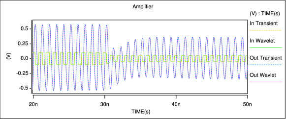
Figure 1: Detail of Input and output signal for the amplifier

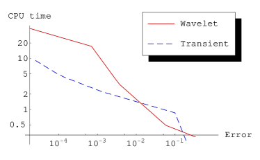
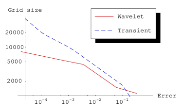
Figure 2: Simulation statistics for the amplifier. Computation time versus error (left), and grid size versus error (right) for transient analysis and adaptive wavelet analysis.

3.2 Oscillator

The oscillator is an autonomous circuit without an external input signal. The simulation runs over 20 ns. As can be seen from Fig 4, an excellent agreement with highly-accurate transient analysis is achieved. It should be noted that after the oscillator has reached its periodic steady state the wavelet method works very fast, since the solution from one interval is an excellent initial guess for the next interval.

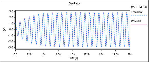
Figure 3: Output signal for the oscillator.

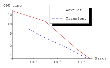
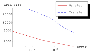
Figure 4: Simulation statistics for the oscillator. Computation time versus error (left), and grid size versus error (right) for transient analysis and adaptive wavelet analysis.

3.3 Mixer

The mixer is simulated with input frequencies 950 MHz and 1GHz. The simulation runs over 30 ns. In particular, for high accuracies the number of degrees of freedom is essentially reduced, while the computation time is at least of the same order.

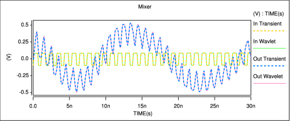
Figure 5: Time domain output signal for the mixer.

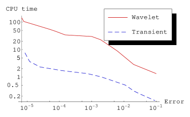
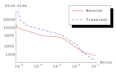
Figure 6: Simulation statistics for the mixer. Computation time versus error (left), and grid size versus error (right) for transient analysis and adaptive wavelet analysis.

4 Conclusion

The results of the simulations indicate that the wavelet based method may achieve and in some cases surpass performance of the standard transient analysis. Apparently, the number of degrees of freedom can be smaller than for the transient analysis for comparable accuracy. However, this advantage of the wavelet algorithm does not always result (yet) in a smaller computation time. On the other hand it can be expected that the productive implementation of the wavelet algorithm can be further optimized. Therefore our activities on optimization and further development of the wavelet-based algorithm are continuing.

- (1) Barthel, A., Knorr, S., Pulch, R.: Wavelet based methods for multirate partial differential-algebraic equations. Appl. Numer. Math. 59, 495–506 (2008)
- (2) Bittner, K.: Biorthogonal spline wavelets on the interval. In: G. Chen, M.J. Lai (eds.) Wavelets and Splines: Athens 2005, pp. 93–104. Nashboro Press, Brentwood, TN (2006)
- (3) Bittner, K., Urban, K.: Adaptive wavelet methods using semiorthogonal spline wavelets: Sparse evaluation of nonlinear functions. Appl. Comput. Harmon. Anal. 24, 94–119 (2008)
- (4) Christoffersen, C., Steer, M.: State-variable-based transient circuit simulation using wavelets. IEEE Microwave and Wireless Components Letters 11, 161–163 (2001)
- (5) Dahmen, W., Schneider, R., Xu, Y.: Nonlinear functionals of wavelet expansions — adaptive reconstruction and fast evaluation. Numer. Math. 86, 49–101 (2000)
- (6) Dautbegovic, E.: Wavelets in circuit simulation. In: J. Roos, L. Costa (eds.) Scientific Computing in Electrical Engineering, Mathematics in Industry, vol. 14, pp. 131–142. Springer, Berlin Heidelberg (2010)
- (7) Dautbegovic, E., Condon, M., Brennan, C.: An efficient nonlinear circuit simulation technique. IEEE Transactions on Microwave Theory and Techniques 53, 548–555 (2005)
- (8) Soveiko, N., Gad, E., Nakhla, M.: A wavelet-based approach for steady-state analysis of nonlinear circuits with widely separated time scales. IEEE Microwave and Wireless Components Letters 17, 451–453 (2007)
- (9) Zhou, D., Cai, W.: A fast wavelet collocation method for high-speed circuit simulation. IEEE Trans. Circuit and Systems 46, 920–930 (1999)
- (10) Zhou, D., Cai, W.: A fast wavelet collocation method for high-speed circuit simulation. IEEE Trans. on Circuits and Systems — I: Fundamental Theory and Appl. 46, 920–930 (1999)