The VMC Survey - XXI. New star cluster candidates discovered from infrared photometry in the Small Magellanic Cloud

Abstract

We report the first search for new star clusters performed using the VISTA near-infrared $YJK_{s}$ Magellanic Clouds survey (VMC) data sets. We chose a pilot field of $\sim$ 0.4 deg² located in the South-West of the Small Magelllanic Cloud (SMC) bar, where the star field is among the densest and highest reddened region in the galaxy. In order to devise an appropriate automatic procedure we made use of dimensions and stellar densities observed in the VMC data sets of the known clusters in this area. We executed different kernel density estimations over a sample of more than 358000 stars with magnitudes measured in the three $YJK_{s}$ filters. We analysed the new cluster candidates whose colour-magnitude diagrams (CMDs), cleaned from field star contamination, were used to assess the clusters’ reality and estimate reddenings and ages of the genuine systems. As a result 38 objects ($\approx$ a 55$\%$ increase in the known star clusters located in the surveyed field) of 0.15 - 0.40 arcmin (2.6 - 7.0 pc) in radius resulted to have near-infrared CMD features which resemble those of star clusters of young to moderate intermediate age (log($t$ yr^-1) $\sim$ 7.5-9.0). Most of the new star cluster candidates are hardly recognizable in optical images without the help of a sound star field decontaminated CMD analysis. For highly reddened star cluster candidates ($E(B-V)$ $\geq$ 0.6 mag) the VMC data sets were necessary in order to recognize them.

1 Introduction

The Magellanic Clouds (MCs) offer us a unique opportunity to study star clusters that have been formed in distinct environments – including age, metallicity, overall gravitational potential, and formation history – in comparison with the star cluster system of the Milky Way, to which we are most familiar with (see van den Bergh, 1991; de Grijs & Anders, 2006; Baumgardt et al., 2013, to trace the developments in the field).

Star clusters in the Large and Small Magellanic Clouds (L/SMC) are spread over many hundreds of square degrees. In comparison, this area is much smaller than the entire sky that must be surveyed for a complete census of the Milky Way’s star clusters, but the distance to the MCs and the crowding from the dense MC field population, make the MC star cluster census a challenging task, subjected to conflicting constraints – it requires deep high angular resolution wide-field imaging.

Today hundreds of SMC star clusters are known (Bica & Dutra, 2000; Bica et al., 2008). The first star cluster searches in the galaxy were carried out nearly a century ago. Shapley & Wilson (1925) compiled a catalog of non-stellar objects, and later Kron (1956) realized that many of them were star clusters.Mohr (1935) reported seven star clusters in the SMC outskirts. Most of the objects in these early lists are prominent enough to have NGC entries.

Kron (1956) and Lindsay (1958) performed special searches aimed at identifying star clusters in the SMC, and indeed they recognized 69 and 116 objects, respectively. Further lists of star clusters were published by Westerlund & Glaspey (1971, 18 objects), Hodge & Wright (1974, 86 objects), and Brück (1976, 168 objects). The compilation of Hodge & Wright (1977) contained 220 star clusters. Hodge (1986) reported 233 new star clusters, and the major effort by Bica & Schmitt (1995) brought the total number of known SMC clusters to 554 – the apex of the star cluster searches based on photographic plates.

The next major step was carried out by Pietrzynski et al. (1998), who utilized the wide field digital imaging in the optical carried out by the Optical Gravitational Lensing Experiment 2 (OGLE2 Paczynski, 1986; Udalski et al., 1997) to search for star clusters within $\sim$2.4 deg² near to the SMC centre. They reported 238 star clusters, 72 of which were new identifications. Most notably, they applied for the first time an automated technique based on surface density maps, following Zaritsky et al. (1997) who used that procedure to search for star clusters in the LMC. Unlike previous efforts that were in effect a simple visual inspection of photographic plates or prints, this method is objective, and is able to assign probabilities to candidates, based on how much they exceed the statistical fluctuations over the background level. Nevertheless, visual inspection of the candidates and their colour-magnitude diagrams (CMDs) are still desirable, because of star clusters embedded in gas clouds might exist. Interestingly, automated methods are much more commonly applied to identify Milky Way’s star clusters: Ivanov et al. (2002); Borissova et al. (2003); Mercer et al. (2005); Froebrich et al. (2007); Koposov et al. (2008).

Bica & Dutra (2000) sumarized the state of the SMC star cluster census at that time. They listed 719 star clusters in total. This number included young star clusters with emission, and loose systems. Later, Bica et al. (2008) updates the SMC star cluster catalogue. A finer re-classification of some objects into star clusters, associations, and shells reduced the number of SMC star clusters to 498. Their properties (e.g., size, age) vary within wide limits, but this discussion is beyond the scope of this paper.

This paper is organised as follows. Section 2 provides an overview of the data sets used in this study and describes the strategy to identify new star clusters. In Section 3 we present the new identified star cluster candidates, the procedure to clean their CMDs from the contamination of field stars and the use of isochrone to determine the clusters’ best-fitting physical parameters. In the same Section we explore the star cluster observed features in both the optical and the near-infrared wavelength ranges. We present our main conclusions in Section 4.

2 strategy for searching new star clusters

In this paper we devise a procedure to search for new star clusters in the SMC with the aim of applying it to the whole VISTA near-infrared $YJK_{s}$ survey of the Magellanic Clouds system (VMC Cioni et al., 2011). VMC is an ESO (European Southern Observatory) public survey that is carried out with the VIRCAM (VISTA InfraRed Camera) instrument (Dalton et al., 2006) on the ESO VISTA telescope (Emerson et al., 2006). The main goals of the survey are to reconstruct the star-formation history (SFH) and its spatial variation, as well as to infer an accurate 3D map of the entire Magellanic system. The VMC survey strategy involves repeated observations of tiles across the Magellanic system, where one tile covers uniformly an area of $\sim$ 1.5 deg², as a result of the mosaic of six paw-print images, in a given waveband with 3 epochs at $Y$ and $J$, and 12 epochs at $K_{s}$. Individual epochs have exposure times of 800 s ($Y$ and $J$) and 750 s ($K_{s}$). The average quality of the VMC data analysed here corresponds to 0.34$\arcsec$ pixel size and 0.90$\arcsec$ FWHM.

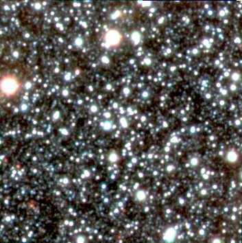
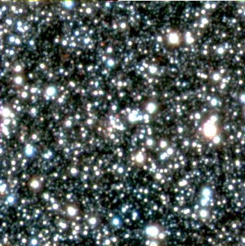
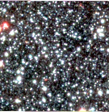
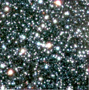
VMC17 VMC18 VMC19 VMC20

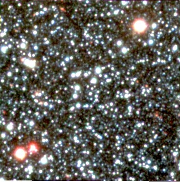
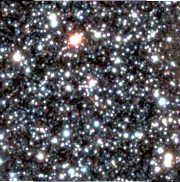
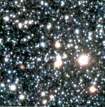
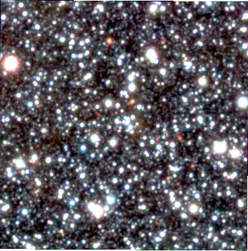
VMC21 VMC22 VMC23 VMC24

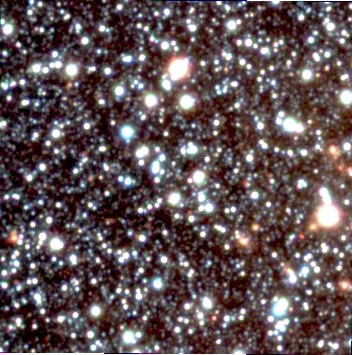
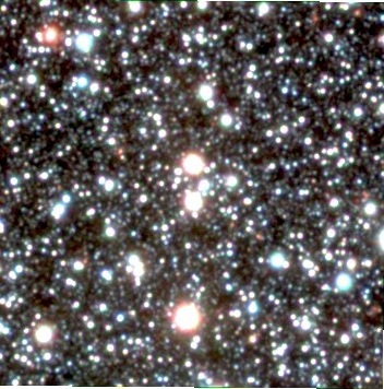
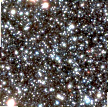
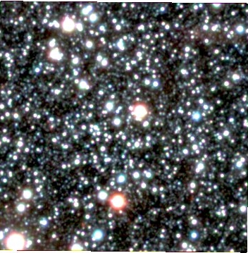
VMC25 VMC26 VMC27 VMC28

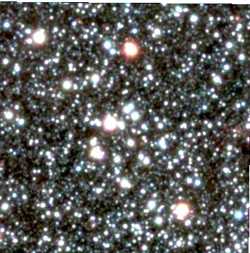
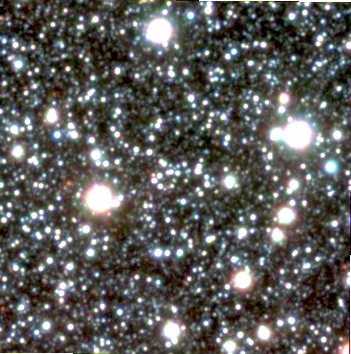
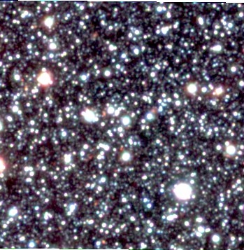
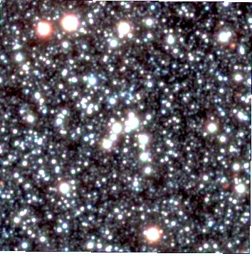
VMC29 VMC30 VMC31 VMC32

Figure 1: continued.

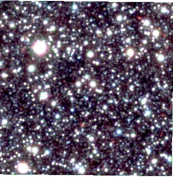
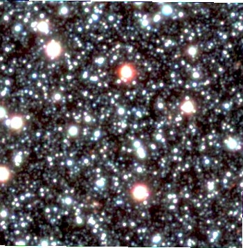
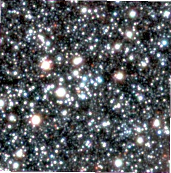
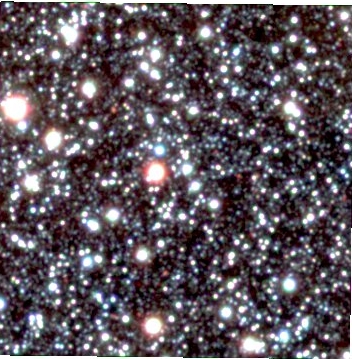
VMC33 VMC34 VMC35 VMC36

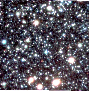
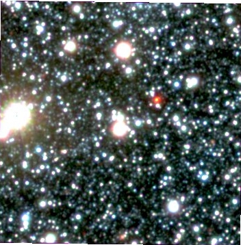
VMC37 VMC38

Figure 1: continued.

We chose a 36$\times$36 arcmin² pilot field located in the South-West part of the SMC bar (see inset chart in Fig. 1) for which we have available images and photometry in the Washington $CT1$ photometric system (Piatti, 2012). These optical images and photometry were used for comparison purposes, i.e., in order to know whether possible new star clusters from the VMC survey were not discovered until now because of the high reddening, the limiting magnitude, the clusters’ sizes and/or the cataloguing technique. The pilot field is likewise one of the densest fields in the galaxy and presents noticeable variations in the stellar density and in the interstellar reddening.

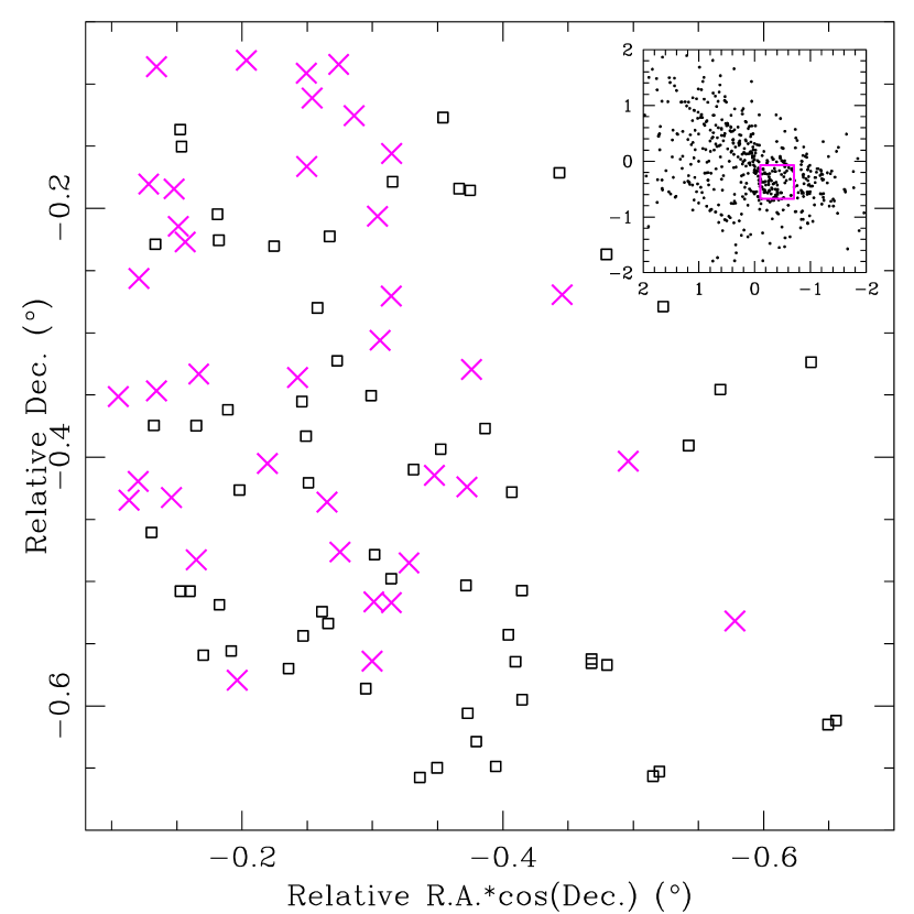
Figure 1: Pilot region chosen to search for new star clusters. Open black squares and magenta crosses represent previoulsy catalogued and new star clusters, respectively. The inset panel depicts the spatial distribution of the catalogued SMC star clusters. A thick magenta-coloured open box delimits the studied SMC field. We used as the SMC centre: RA = 00h 52m 45s, Dec = $-$72$\degr$ 49$\arcmin$ 43$\arcsec$ (J2000) (Crowl et al., 2001).

The Washington $CT_{1}$ images of the seleted field were obtained at the Cerro Tololo Inter-American Observatory 4-m Blanco telescope with the Mosaic II camera attached (a 8K$\times$8K CCD detector array) and are available at the National Optical Astronomy Observatory (NOAO) Science Data Management Archives. The 50 per cent completeness level of the resulting photometry is located at a $T_{1}$ magnitude and a $C-T_{1}$ colour corresponding to the Main Sequence (MS) turnoff of a stellar population with an age $\ga$ 10 Gyr. This photometric data set was used to estimate fundamental parameters of star clusters (Piatti, 2011; Maia et al., 2014), to trace the field age-metallicity relationship (Piatti, 2012), to develop a procedure to clean the clusters’ CMDs from the unavoidable star field contamination (Piatti & Bica, 2012), among others.

From the VMC survey, we used the region of the tile SMC 4$\_$3 which fully contains the selected field. All data used in this work were produced as in the SFH study performed by Rubele et al. (2015), where data acquisition and reduction, point-spread-function photometry and artificial star tests for completeness assessment are extensively described. Those VMC tile SMC 4$\_$3 data (88% of completion) were used to trace a reddening map throughout the tile, to investigate the SMC depth along the line-of-sight, to build a look back time star formation rate and a mass tomography (Rubele et al., 2015). The reduced data for this tile used here (100% of completion) will be released to the community together with the data for other tiles as part of data release #5 which is planned for 2016. All sources detected are not saturated, so that there are no stars missed at the bright part of the CMDs that may influence the subsequent star cluster analysis, contrarily to what was suggested by Bica et al. (2015). The 50 per cent completeness level reached in the $K_{s}$ mag and the $Y-K_{s}$ colour corresponds to the MS turnoff of a stellar population with an age of $\sim$ 6 Gyr old.

We built a list of 68 star clusters located in the region from the the catalogue of Bica et al. (2008). These catalogued star clusters are not always straightforward to identify in deep VMC tile images. This is because they were originally identified from optical images (e.g. from the Digitized Sky Survey, DSS, images) which can look rather different compared with their appearance at near-infrared wavelengths. Furthermore, they were identified using images with different spatial resolutions and depth than the VMC ones. Consequently, some misidentification might occur. For instance, single relatively bright stars might look like an unresolved compact star cluster in images of lower spatial resolution, or unresolved background galaxies could be mistaken for small star clusters in shallower images. Fig. 1 depicts with open squares the spatial distribution of star clusters catalogued by Bica et al. (2008) in the selected region. Because of the higher surface brightness of the background and the more populous nature of this SMC bar region, star clusters stand out less, and incompleteness effects are expected to be more important than in the outer regions of the galaxy.

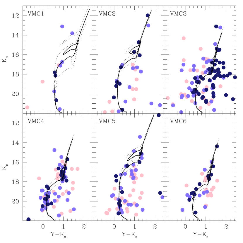
Figure 2: $K_{s}$ versus $Y-K_{s}$ CMD of stars within the cluster radius. Colour-coded symbols represent stars that statistically belong to the field ($P\leq$ 25%, pink), stars that might belong to either the field or the cluster ($P=$ 50%, light blue), and stars that predominantly populate the cluster region ($P\geq$ 75%, dark blue). Three isochrones from Bressan et al. (2012) for log($t$ yr^-1) and log($t$ yr^-1) $\pm$ 0.1 are also superimposed.

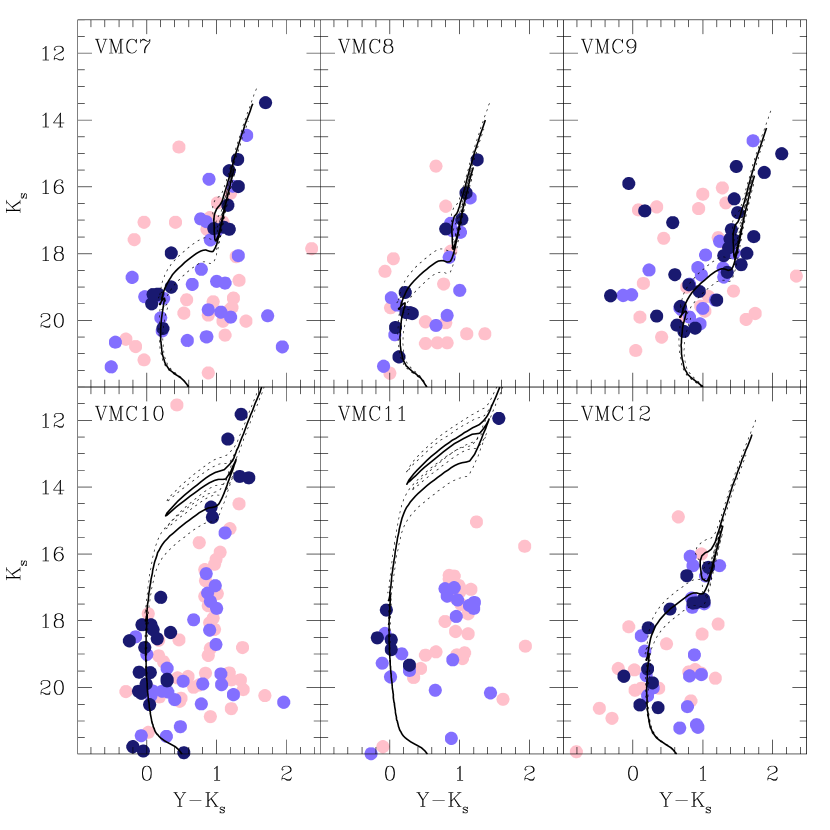
Figure 2: continued.

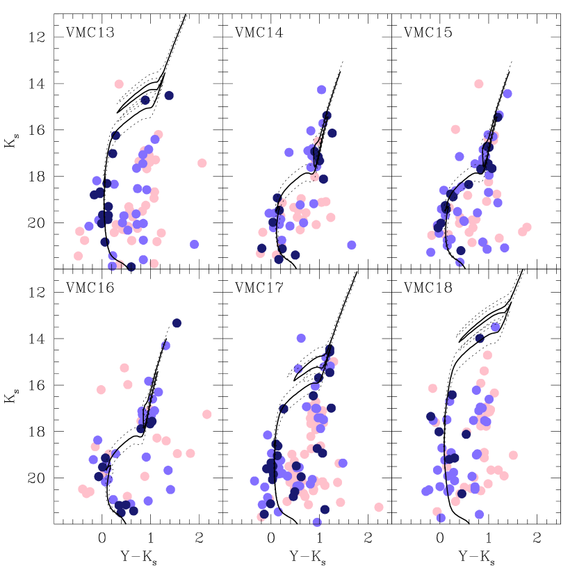
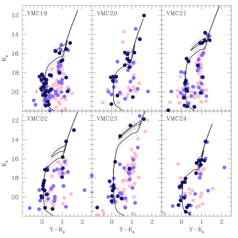
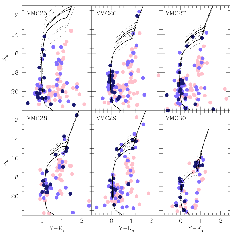
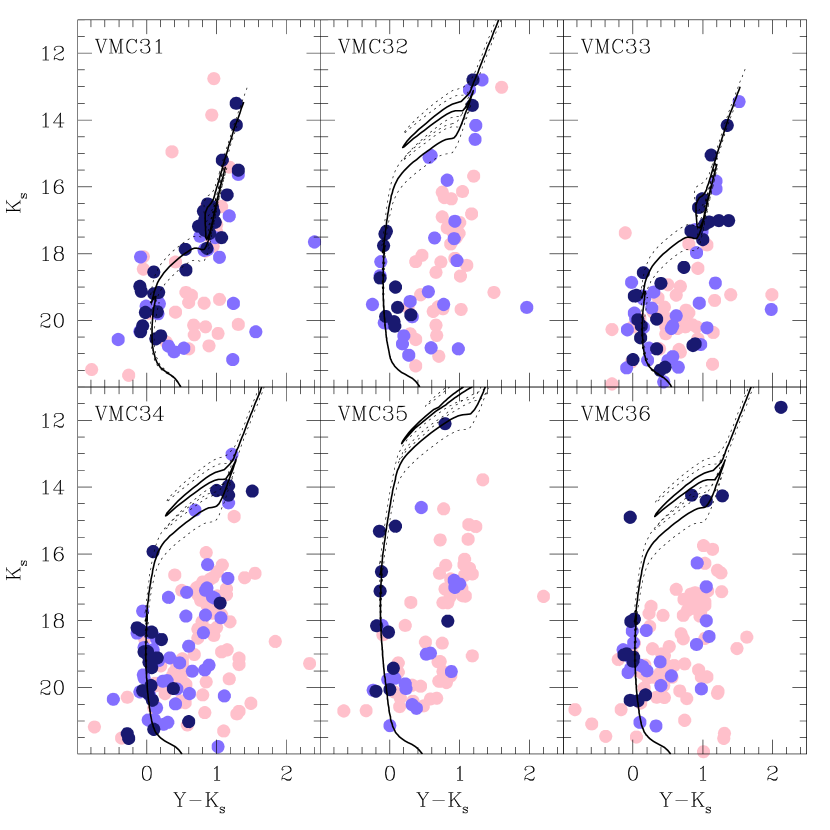
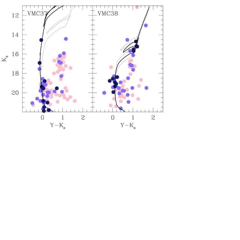
Figure 2: continued.

We first overplotted the positions of the catalogued star clusters on the deepest Washington $T_{1}$ and VMC $K_{s}$ images, and visually recognized them in both the optical and near-infrared regimes. Note that the main aim of this task is to confirm the given star cluster coordinates in order to properly count the number of stars inside the clusters’ radii from the VMC PSF photometry. Fig. 2 shows the resulting mean stellar densities as a function of the star clusters’ radii -taken from Bica et al. (2008)- for the catalogued star clusters in the surveyed region (open squares). The counts were carried out by considering only stars with magnitude measures in the three $YJK_{s}$ filters. The range of values of both quantities -radii and stellar densities- were used as input information in the procedure of search for star clusters using the VMC data set.

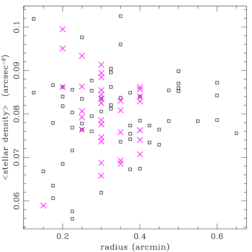
Figure 2: Relationship between the stellar density and the cluster radius in the studied SMC field. The typical background stellar density ranges between 0.008 and 0.012 arcsec^-2. Open black squares and magenta crosses represent previoulsy catalogued and new star cluster candidates, respectively.

The search was performed by employing AstroML routines (Vanderplas et al., 2012, and reference therein for a detail description of the complete AstroML package and user’s Manual), a machine learning and data mining for Astronomy package. AstroML is a Python module for machine learning and data mining built on numpy, scipy, scikit-learn, matplotlib, and astropy, and distributed under the 3-clause BSD license. It contains a growing library of statistical and machine learning routines for analysing astronomical data in Python, loaders for several open astronomical datasets, and a large suite of examples of analysing and visualizing astronomical datasets. The goal of AstroML is to provide a community repository for fast Python implementations of common tools and routines used for statistical data analysis in astronomy and astrophysics, to provide a uniform and easy-to-use interface to freely available astronomical data sets.

We used two different Kernel Density Estimators (KDEs) from six available in AstroML, namely, Gaussian and tophat, and three different bandwidths (the FWHM/2 of the KDE) for each KDE of 0.23, 0.45 and 0.68 arcmin, respectively, thus uniformly sampling the range of known star clusters’ radii (see Fig. 2). A KDE is a non-parametric density estimation technique which alleviates the problem of the histogram dependence on the bin size and the end points of bins by centering a function (kernel) to each data point and then add them up (Rosenblatt, 1956). The result is a continuous density distribution - instead of a not smooth blocky histogram - that allows to extrat the finest structures of it. In our case, we generated a stellar density surface over the studied region. In total, we run six different kernel overdensity searches on a sample of 358578 stars with positions and magnitudes measured in the three $YJK_{s}$ filters. From the total number of overdensities detected respect to their local backgrounds per search, we imposed a cut off density of 0.05 arcsec^-2 in order to keep only star cluster candidades within the density range seen in Fig. 2 for the known star clusters. The typical background stellar density ranges between 0.008 and 0.012 arcsec^-2, so that we only keep overdensities at least $\sim$ 5 times higher. Indeed, we identified all the 68 known clusters from the VMC data set, which resulted to be overdensities higher than 0.05 arcsec^-2 (see Fig. 2). Note that the performance of the technique in identifying star clusters depends on the chosen density cut off, bandwidths and KDE functions. Based on the selection criteria mentioned above, we used the most suitable ones in order to identify the 68 known star clusters and new cluster candidates as well. We merged the resulting lists, avoiding repeated overdensities from different runs. We also discarded the recovered 68 known star clusters and visually inspected the star cluster candidates on the deepest $K_{s}$ image. This is a conservative exploration, since star clusters embedded in clouds could exist and no overdensity would come out from this search (Romita et al., 2016). We finally got 143 star cluster candidates.

3 results and discussion

The new 143 apparent stellar concentrations found from the VMC data set do not necessarily assure us that they constitute physical systems. Piatti & Bica (2012) showed evidence that some SMC candidate star clusters are in fact not genuine physical systems. According to the authors, nearly 10 per cent of their studied star cluster sample resulted in possible non-clusters. This does not seem to be a significant percentage of the catalogued star clusters. Indeed, they used the spatial distribution of possible non-clusters in the SMC to statistically decontaminate that of the SMC star cluster system. By assuming that the area covered by them represents an unbiased subsample of the SMC as a whole and by using an elliptical framework centred on the SMC centre, they found that there is no significant difference between the expected and observed star cluster spatial distributions. However, a difference at a 2$\sigma$ level would become visible between $a$ $\approx$ 0$\degr$.3 and 1$\degr$.32 (the semi-major axis of an ellipse parallel to the SMC bar and with $b/a$ = 1/2), if the possible non-clusters were increased up to 20 per cent. For the 143 new star cluster candidates, we used their CMDs to infer the existence of genuine star clusters.

When dealing with small objects or sparse star clusters projected or immersed in crowded star fields, as those star clusters located in the inner regions of the SMC, a simple circular CMD extraction around the star cluster centre could lead to a wrong conclusion, since the CMDs are obviously composed of stars of different stellar populations (Piatti, 2012). Consequently, it is hardly possible to assess whether bright and young MSs or subgiant and red giant branches trace the fiducial star cluster features. In order to statistically clean the star cluster CMDs from the unavoidable field contamination we applied a procedure developed by Piatti & Bica (2012), which has proved to be useful in previous papers, among them, from the VMC data sets (see, e.g. Piatti et al., 2014; Piatti et al., 2015a; Piatti et al., 2015b). In short, the star field cleaning relies on the comparison of each of four previously defined field CMDs to the cluster CMD and subtracted from the latter a representative field CMD in terms of stellar density, luminosity function, and colour distribution. This was done by comparing the numbers of stars counted in boxes distributed in a similar manner throughout all CMDs. The boxes were allowed to vary in size and position throughout the CMDs in order to meaningfully represent the actual distribution of field stars.

Since we repeated this task for each of the four field CMDs, we could assign a membership probability to each star in the cluster CMD. This was done by counting the number of times a star remained unsubtracted in the four cleaned cluster CMDs and by subsequently dividing this number by 4. Thus, we distinguished field populations projected on to the star cluster area, i.e. those stars with a probability $P\leq$ 25 per cent, stars that could equally likely be associated with either the field or the object of interest ($P=$ 50 per cent), and stars that are predominantly found in the cleaned star cluster CMDs ($P\geq$ 75 per cent) rather than in the field star CMDs. Statistically speaking, a certain amount of cleaning residuals is expected, which depends on the degree of variability of the stellar density, luminosity function and colour distribution of the field stars. We employed this field star decontamination procedure to clean circular areas of 1.2 arcmin in radius around the central coordinates of the 143 new star cluster candidates using both Washington and VMC data sets. Here we took advantage of the Washington CMDs for comparison purposes, thus allowing us to know from the optical regime how cluster candidates identified from the near-infrared behave. Note that we do not use the Washington photometry to infer the object reality. As a result 38 objects turned out to have cleaned near-infrared CMDs with features (stars with $P\geq$ 50 per cent) which resemble those of star clusters of young to moderate intermediate age (log($t$ yr^-1) $\sim$ 7.5-9.0). Cleaned CMDs without any detectable trace of star cluster sequences were discarded.

The star cluster radii used to extract their CMDs were taken from a visual inspection of the deepest $K_{s}$ image, and were meant to allow us to meaningfully define the clusters’ fiducial sequences in their CMDs. The number of new star cluster candidates represents about a 55$\%$ increase in the number of known star clusters located in the surveyed region, which is a significant percentage in terms of the currently debateable issues about the star cluster formation rate, the effectiveness of star cluster dissolution processes, etc (Glatt et al., 2011; Piatti, 2014; Chandar et al., 2015, and references therein). Such a number could be still higher if we carried out a search not as conservative as that developed in this paper, i.e., not constrained to a range of stellar densities (e.g. embedded star clusters Romita et al., 2016). Note that we do not aim at building a complete list of star clusters, but rather to devise a method useful to identify star clusters making use of KDEs and, in turn, to introduce the first star cluster candidates discovered in the SMC based on such a procedure. It would be worth to apply the present analysis tools to search for faint poorly populated star clusters in the Magellanic Clouds using deep images obtained by, for example, 8-m class telescopes.

Figures 1 and 2 show the positions in the galaxy of these new star cluster candidates and the relationship between their stellar densities and dimensions, respectively. We have highlighted them with magenta-coloured crosses. Note that they do not reveal any particular spatial distribution pattern, but spread over the surveyed field. Likewise, their observed stellar densities are within the range of those of known star clusters in the region. This is a expected result, because of the imposed cut off density limit and the KDE’s bandwidths used. The identification of new star cluster candidates shows that the automatic search performed here has some advantages over those previous carried out by visually inspecting photographic plates (e.g. Bica & Schmitt, 1995) or by other automatic algorithmic searches (e.g. Pietrzynski et al., 1998). In Figure A1 of the Appendix we present 2$\times$2 arcmin² $YJK_{s}$ images centred on the new SMC star cluster candidates, where it can be seen the environment within which they are inmersed. Note that the displayed fields are nearly 7 times larger in radius respect to the clusters’ sizes. Although the star clusters are centred on the images, the distribution of field stars along the line of sight as well as the scale of brightness used to produce the images might lead the reader to confuse them with groups of bright field stars and/or clouds of gas/dust. We recall that the new star cluster candidates are identified not only as stellar overdenssities but also from their field star cleaned CMDs.

We estimated reddening values and ages for our 38 new star cluster candidates using the theoretical isochrones of Bressan et al. (2012) in the Vegamag system (where, by definition, Vega has a magnitude of zero in all filters), corrected by -0.074 mag in $Y$ and -0.003 mag in $K_{s}$ to put them on the VMC system (Rubele et al., 2015), to match the cleaned star cluster CMDs. We adopted the same distance modulus for all star clusters $(m-M)_{o}$ = 18.9 $\pm$ 0.1 mag and $K_{s}-M_{K_{s}}=(m-M)_{o}+0.372\times E(B-V)$, for $R_{V}=3.1$ (Cardelli et al., 1989; Gao et al., 2013), since changes in the distance modulus by an amount equivalent to the average depth for this SMC region derived by Rubele et al. (2015, see their Fig. 8), leads to a smaller age difference than that resulting from the isochrones (characterized by the same metallicity) bracketing the observed star cluster features in the CMD. We chose isochrones for $Z$ = 0.003 ([Fe/H] = -0.7 dex), which corresponds to the mean SMC star cluster metal content for the last $\sim$ 2-3 Gyr (Piatti & Geisler, 2013). Note that the $Y-K_{s}$ colour is not sensitive to metallicity differences smaller than $\Delta$[Fe/H] $\sim$ 0.4 dex, which is adequate given the spread of the stars in the CMDs (see Piatti et al., 2015a).

We found in general that isochrones bracketing the derived mean age by $\Delta$log($t$ yr^-1) = $\pm$0.1 represent the overall uncertainties associated with the observed dispersion in the cluster CMDs. Although the dispersion is smaller in some cases, we prefer to retain the former values as an upper limit to our error budget. VMC1, 25 and 37 deserved particular attention. These object fields have few relatively bright stars with $P\geq$ 50 per cent, so that instead of deriving their ages we only could estimate older age limits. As for reddening errors we found a slight correlation with the derived $E(B-V)$ values which, in some cases, could be related to the presence of differential reddening. For star clusters with $E(B-V)\leq$ 0.35 mag, the reddening uncertainty is estimated as 0.05 mag while for star clusters with larger $E(B-V)$ values, the uncertainty reaches 0.10 mag. These reddening uncertainties are thought to mainly represent the overall dispersion along the star cluster CMD features, rather than a measure of the total reddening spread. Nevertheless, in most of the star clusters the adopted reddening uncertainties fairly reflect the observed MS broadness, thus implying that only some star clusters show clear effects of differential reddening. VMC3 presents differential reddening of $\la$ 0.5 mag, and we used the lower value $E(B-V)$ = 0.7 mag to match the isochrones. Table 1 lists the adopted central coordinates, radii, the resulting reddening and age values, and the number of stars with $P\geq$ 75 per cent. The latter is meant to provide an estimate of the cluster candidate populousness, although some outliers are included. Fig. A2 of the Appendix illustrates the results of the isochrone matching for the entire new star cluster candidate sample.

Table 1: Fundamental parameters of new SMC star clusters.

Name	R.A.	Dec.	$r$	$E(B-V)$	log($t$)	Na
	(°)	(°)	(’)	(mag)
VMC1	11.169	-73.360	0.15	0.90	$<$8.4$\pm$0.3	3
VMC2	11.468	-73.232	0.20	0.40	8.5	10
VMC3	11.655	-73.098	0.40	0.70	9.0	55
VMC4	11.890	-73.158	0.30	0.30	8.9	22
VMC5	11.895	-73.253	0.30	0.50	8.4	12
VMC6	11.982	-73.243	0.20	0.50	9.0	14
VMC7	12.045	-73.314	0.30	0.35	8.9	16
VMC8	12.090	-73.345	0.20	0.25	9.0	10
VMC9	12.106	-73.099	0.30	0.90	9.0	23
VMC10	12.112	-72.984	0.40	0.25	8.1	25
VMC11	12.133	-73.135	0.25	0.30	7.8	6
VMC12	12.137	-73.345	0.25	0.40	8.7	13
VMC13	12.139	-73.392	0.30	0.30	8.2	16
VMC14	12.146	-73.035	0.25	0.25	8.9	13
VMC15	12.212	-72.954	0.30	0.25	8.9	16
VMC16	12.229	-73.305	0.25	0.20	9.0	11
VMC17	12.254	-72.913	0.35	0.30	8.4	19
VMC18	12.267	-73.265	0.30	0.40	7.9	8
VMC19	12.323	-72.940	0.40	0.35	8.5	35
VMC20	12.334	-72.995	0.30	0.25	8.7	16
VMC21	12.338	-72.920	0.35	0.45	8.3	19
VMC22	12.349	-73.165	0.30	0.30	8.4	18
VMC23	12.427	-73.234	0.35	0.40	7.8	15
VMC24	12.496	-72.910	0.25	0.20	8.7	18
VMC25	12.500	-73.408	0.40	0.30	$<$7.6$\pm$0.4	17
VMC26	12.612	-73.162	0.40	0.20	8.1	18
VMC27	12.613	-73.311	0.40	0.20	8.1	23
VMC28	12.650	-73.056	0.30	0.40	8.3	16
VMC29	12.669	-73.043	0.40	0.30	8.2	16
VMC30	12.681	-73.261	0.25	0.15	8.8	13
VMC31	12.681	-73.013	0.35	0.20	8.9	30
VMC32	12.723	-73.175	0.30	0.15	8.1	12
VMC33	12.730	-72.915	0.30	0.30	8.8	26
VMC34	12.748	-73.009	0.40	0.25	8.1	27
VMC35	12.770	-73.248	0.30	0.20	7.5	11
VMC36	12.771	-73.085	0.35	0.30	8.1	14
VMC37	12.793	-73.263	0.30	0.25	$<$7.3$\pm$0.5	12
VMC38	12.824	-73.180	0.30	0.35	8.4	14

^a Number of stars within the cluster radius with $P\geq$ 75 per cent.

The Washington cleaned CMDs around the central positions of the new star clusters allow us to know their observed features in the optical wavelength regime and consequently, to compare them to those in the near-infrared. By doing this exercise, we found that most of the star clusters are detectable from a sound Washington CMD analysis, once the star field signature is properly filtered. We used the derived reddenings and ages of Table 1, as well as a distance modulus $(m-M)_{o}$ = 18.9 and a metallicity of $Z$ = 0.003, to match theoretical isochrones (Bressan et al., 2012) to the cleaned $T_{1}$ versus $C-T_{1}$ CMDs. The theoretical isochrones were properly shifted by the corresponding $E(C-T_{1})=1.97E(B-V)$ colour excesses and by the SMC distance modulus $T_{1}=M_{T_{1}}+(m-M)_{o}+2.62E(B-V)$ (Geisler & Sarajedini, 1999). We confirmed our estimated values of $E(B-V)$ and log($t$ yr^-1), as illustrated in Fig. 3. As can be seen, the Washington photometry is slightly deeper than the VMC one and possibly, due to a relatively low reddening along the line-of-sight, the generally blue integrated light nature of young/moderate age star clusters makes their MS appear reasonably well-populated. At the top of Fig. 3 we show the deepest $C$, $T_{1}$ and $K_{s}$ images (from left ot right) of the star cluster field. Note that the star cluster clearly stands out at the near-infrared image, while it is hardly possible to recognize it from the optical one without the help of the corresponding CMD analysis.

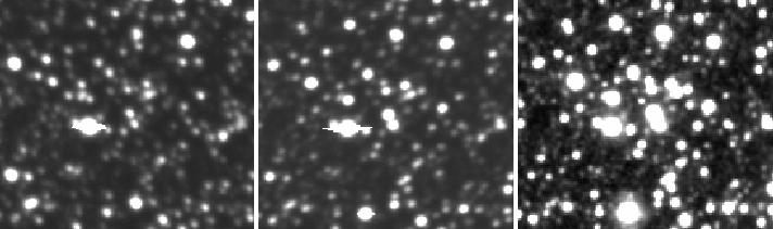
Figure 3: Top: $C$, $T_{1}$ and $K_{s}$ images (from left to right) centred on the new star cluster candidate VMC17. The images’ sides are equal to the star cluster diameter (see Table 1). North is up and East to the left. Bottom: Washington and VMC CMDs illustrating the performance of the cleaning procedure, where we plotted all the measured stars located within the cluster radius. The pink, light and dark blue filled circles in the bottom panels represent stars with cluster membership probabilities $P\leq$ 25 per cent, $P=$ 50 per cent, and $P\geq$ 75 per cent, respectively. Three isochrones from Bressan et al. (2012) for log($t$ yr^-1) = 8.3, 8.4, and 8.5 and $Z$ = 0.003 are also superimposed.

Three cluster candidates (VMC 1, 3 and 9), on the other hand, could not be identified neither by a visual inspection of their $C,T_{1}$ images nor from the respective cleaned CMDs. We found that all of them are affected by reddening higher than $E(B-V)$ $\sim$ 0.6 mag, so that we conclude that this could be the reason for making them undetectable from optical photometry. Fig. 4 illustrates this situation, in which the 1 Gyr old star cluster candidate VMC9 appears hidden at optical wavelengths. This example, in turn, brings support to our original motivation for this search, in the sense that the VMC survey should have imaged those star clusters that are either behind or embedded within clouds in the Magellanic system. According to Rubele et al. (2015), who produced an $A_{V}$ extinction map for the SMC main body, our pilot field is the most reddened in the galaxy, with best-fitting $E(B-V)$ values larger than 0.20 mag. Their $A_{V}$ extinction map was built by running the StarFISH SFH-recovery software over a wide-enough grid of distance modulus and extinction values until the code returns not only the best-fitting coefficients for the SFH, but also the best-fitting ($(m-M)_{o},A_{V}$) pair (see their Fig. 11).

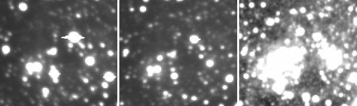
Figure 4: Same as Fig. 3 for the new star cluster candidate VMC9. Three isochrones from Bressan et al. (2012) for log($t$ yr^-1) = 8.9, 9.0, and 9.1 and $Z$ = 0.003 are also superimposed.

4 conclusions

By using the near-infrared VMC data set we performed a search for new star clusters in the South-West side of the SMC bar, where the star field is the densest and hightest reddened region in the galaxy. The search was motivated by the fact that star clusters not seen in the visible could be dwelling such regions, as judged by the comparison of optical and VMC images.

The devised procedure for the star cluster search relies on astrophysical information taken from the VMC PSF photometric catalogues for the known star clusters located in a pilot field of $\sim$ 0.4 deg². From the learned distribution of the dimensions and the observed stellar densities of known star clusters, we designed a strategy for finding new ones that consisted in using Gaussian and tophat KDEs for three different bandwidths. After perfoming six different runs over an amount of 358578 stars with measurements in the three $YJK_{s}$ filters, we detected 143 new star cluster candidates, within a similar range of radius and stellar density to the previously catalogued star cluster sample.

We applied a subtraction procedure developed by Piatti & Bica (2012) to statistically clean the star cluster CMDs from field star contamination in order to disentangle star cluster features from those belonging to their surrounding fields. The employed technique makes use of variable cells in order to reproduce the field CMD as closely as possible. As a result 38 objects of relatively small size - on average $\sim$ 0.3 arcmin in radius - resulted to have near-infrared CMD features which resemble those of star clusters of young to moderate intermediate age (log($t$ yr^-1) $\sim$ 7.5-9.0). The new star cluster candidates represent $\approx$ a 55$\%$ increase on the known star cluster population, which is particularly significant in the light of the current debates about the star cluster formation rate, the effectiveness of star cluster dissolution processes, etc.

From matching theoretical isochrones computed for the VISTA system to the cleaned star cluster CMDs we estimated reddenings and ages. When adjusting a subset of isochrones we took into account the SMC distance modulus and the mean SMC star cluster metal content for the last $\sim$ 2-3 Gyr. The derived mean $E(B-V)$ colour excesses are in between 0.15 mag and 0.90 mag, while their ages are in the range 7.3 $\leq$ log($t$ yr^-1) $\leq$ 9.0. This new star cluster candidate sample will be part of the cluster database that the VMC survey will produce in order to homogeneously study the overall star cluster formation history throughout the Magellanic system.

When comparing the cleaned star cluster CMDs obtainted from $CT_{1}$ Washington photometry, by employing the same star field decontamination method mentioned above, to those from the VMC survey, we found that most of the new star clusters are detectable, and confirm our estimates of $E(B-V)$ and log($t$ yr^-1). Likewise, it is worth mentioning that the star clusters are clearly visible in the deepest $K_{s}$ images, whereas it is hardly possible to recongnize them from the optical ones without the help of the corresponding CMD analysis. Whenever the star clusters are affected by reddening higher than $E(B-V)$ $\geq$ 0.6 mag, they could not be recognized from the analysis of Washington photometry, thus supporting the crucial complementary role of near-infrared bands surveys.

Appendix A New SMC star clusters

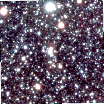
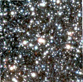
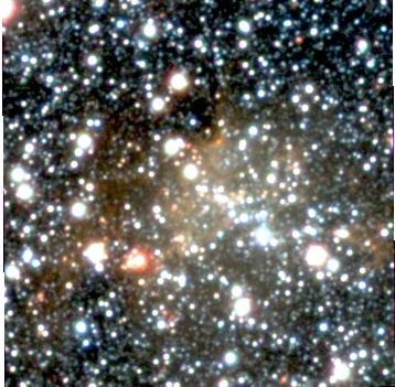
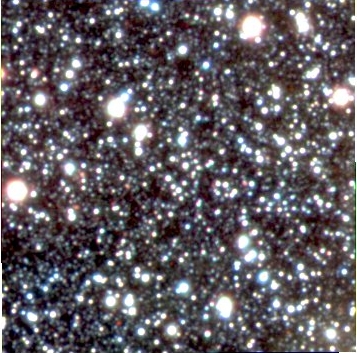
VMC1 VMC2 VMC3 VMC4

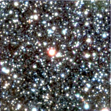
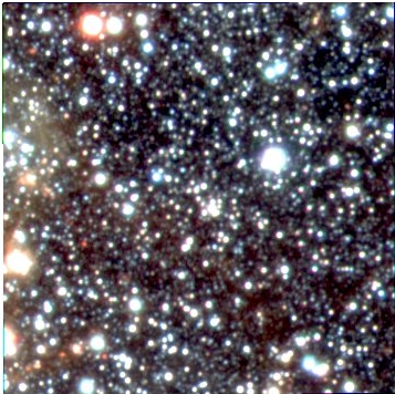
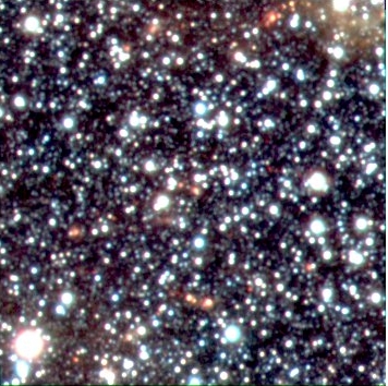
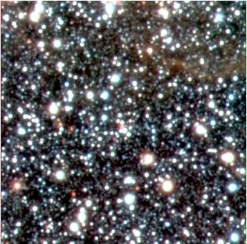
VMC5 VMC6 VMC7 VMC8

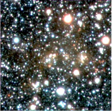
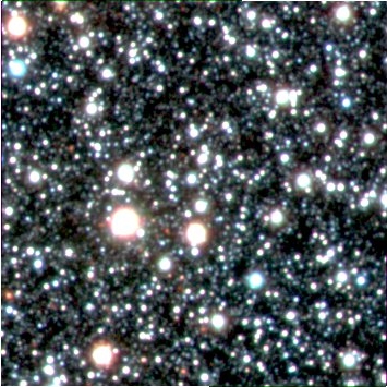
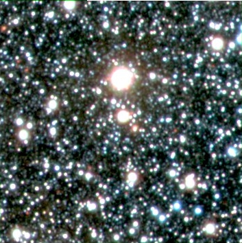
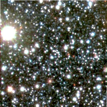
VMC9 VMC10 VMC11 VMC12

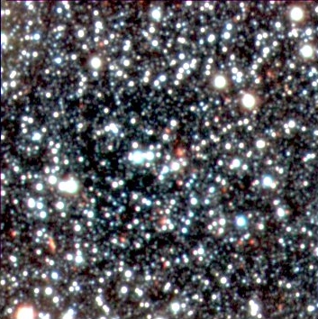
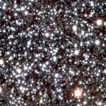
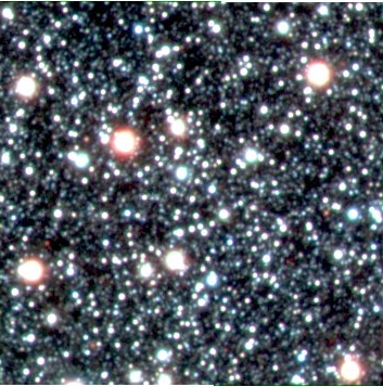
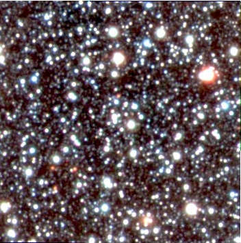
VMC13 VMC14 VMC15 VMC16

Figure 5: 2$\times$2 arcmin² $YJK_{s}$ images centred on the new SMC star clusters. North is up and East to the left. Note that the star clusters’ radii are between 0.15 and 0.40 arcmin.

Figure 2: continued.

Figure 2: continued.

Figure 2: continued.

Figure 2: continued.

References

- Baumgardt et al. (2013) Baumgardt H., Parmentier G., Anders P., Grebel E. K., 2013, MNRAS, 430, 676
- Bica & Dutra (2000) Bica E., Dutra C. M., 2000, AJ, 119, 1214
- Bica & Schmitt (1995) Bica E. L. D., Schmitt H. R., 1995, ApJS, 101, 41
- Bica et al. (2008) Bica E., Bonatto C., Dutra C. M., Santos J. F. C., 2008, MNRAS, 389, 678
- Bica et al. (2015) Bica E., Santiago B., Bonatto C., Garcia-Dias R., Kerber L., Dias B., Barbuy B., Balbinot E., 2015, MNRAS, 453, 3190
- Borissova et al. (2003) Borissova J., Pessev P., Ivanov V. D., Saviane I., Kurtev R., Ivanov G. R., 2003, A&A, 411, 83
- Bressan et al. (2012) Bressan A., Marigo P., Girardi L., Salasnich B., Dal Cero C., Rubele S., Nanni A., 2012, MNRAS, 427, 127
- Brück (1976) Brück M. T., 1976, Occasional Reports of the Royal Observatory Edinburgh, 1
- Cardelli et al. (1989) Cardelli J. A., Clayton G. C., Mathis J. S., 1989, ApJ, 345, 245
- Chandar et al. (2015) Chandar R., Fall S. M., Whitmore B. C., 2015, ApJ, 810, 1
- Cioni et al. (2011) Cioni M.-R. L., et al., 2011, A&A, 527, A116
- Crowl et al. (2001) Crowl H. H., Sarajedini A., Piatti A. E., Geisler D., Bica E., Clariá J. J., Santos Jr. J. F. C., 2001, AJ, 122, 220
- Dalton et al. (2006) Dalton G. B., et al., 2006, in Society of Photo-Optical Instrumentation Engineers (SPIE) Conference Series. p. 0, doi:10.1117/12.670018
- Emerson et al. (2006) Emerson J., McPherson A., Sutherland W., 2006, The Messenger, 126, 41
- Froebrich et al. (2007) Froebrich D., Scholz A., Raftery C. L., 2007, MNRAS, 374, 399
- Gao et al. (2013) Gao J., Jiang B. W., Li A., Xue M. Y., 2013, ApJ, 776, 7
- Geisler & Sarajedini (1999) Geisler D., Sarajedini A., 1999, AJ, 117, 308
- Glatt et al. (2011) Glatt K., et al., 2011, AJ, 142, 36
- Hodge (1986) Hodge P., 1986, PASP, 98, 1113
- Hodge & Wright (1974) Hodge P. W., Wright F. W., 1974, AJ, 79, 858
- Hodge & Wright (1977) Hodge P. W., Wright F. W., 1977, The Small Magellanic Cloud
- Ivanov et al. (2002) Ivanov V. D., Borissova J., Pessev P., Ivanov G. R., Kurtev R., 2002, A&A, 394, L1
- Koposov et al. (2008) Koposov S. E., Glushkova E. V., Zolotukhin I. Y., 2008, A&A, 486, 771
- Kron (1956) Kron G. E., 1956, PASP, 68, 125
- Lindsay (1958) Lindsay E. M., 1958, MNRAS, 118, 172
- Maia et al. (2014) Maia F. F. S., Piatti A. E., Santos J. F. C., 2014, MNRAS, 437, 2005
- Mercer et al. (2005) Mercer E. P., et al., 2005, ApJ, 635, 560
- Mohr (1935) Mohr J., 1935, Harvard College Observatory Bulletin, 899, 15
- Paczynski (1986) Paczynski B., 1986, ApJ, 304, 1
- Piatti (2011) Piatti A. E., 2011, MNRAS, 418, L69
- Piatti (2012) Piatti A. E., 2012, MNRAS, 422, 1109
- Piatti (2014) Piatti A. E., 2014, MNRAS, 437, 1646
- Piatti & Bica (2012) Piatti A. E., Bica E., 2012, MNRAS, 425, 3085
- Piatti & Geisler (2013) Piatti A. E., Geisler D., 2013, AJ, 145, 17
- Piatti et al. (2014) Piatti A. E., et al., 2014, A&A, 570, A74
- Piatti et al. (2015a) Piatti A. E., de Grijs R., Rubele S., Cioni M.-R. L., Ripepi V., Kerber L., 2015a, MNRAS, 450, 552
- Piatti et al. (2015b) Piatti A. E., et al., 2015b, MNRAS, 454, 839
- Pietrzynski et al. (1998) Pietrzynski G., Udalski A., Kubiak M., Szymanski M., Wozniak P., Zebrun K., 1998, Acta Astron., 48, 175
- Romita et al. (2016) Romita K., Lada E., Cioni M.-R., 2016, preprint, (arXiv:1601.07042)
- Rosenblatt (1956) Rosenblatt M., 1956, The Annals of Mathematical Statistics, 27, 832
- Rubele et al. (2015) Rubele S., et al., 2015, preprint (arXiv:1501.05347)
- Shapley & Wilson (1925) Shapley H., Wilson H. H., 1925, Harvard College Observatory Circular, 276, 1
- Udalski et al. (1997) Udalski A., Kubiak M., Szymanski M., 1997, Acta Astron., 47, 319
- Vanderplas et al. (2012) Vanderplas J., Connolly A., Ivezić Ž., Gray A., 2012, in Conference on Intelligent Data Understanding (CIDU). pp 47 –54, doi:10.1109/CIDU.2012.6382200
- Westerlund & Glaspey (1971) Westerlund B. E., Glaspey J., 1971, A&A, 10, 1
- Zaritsky et al. (1997) Zaritsky D., Harris J., Thompson I., 1997, AJ, 114, 1002
- de Grijs & Anders (2006) de Grijs R., Anders P., 2006, MNRAS, 366, 295
- van den Bergh (1991) van den Bergh S., 1991, ApJ, 369, 1