Abstract

The instability in the selection of models is a major concern with data sets containing a large number of covariates. We focus on stability selection which is used as a technique to improve variable selection performance for a range of selection methods, based on aggregating the results of applying a selection procedure to sub-samples of the data where the observations are subject to right censoring. The accelerated failure time (AFT) models have proved useful in many contexts including the heavy censoring (as for example in cancer survival) and the high dimensionality (as for example in micro-array data). We implement the stability selection approach using three variable selection techniques—Lasso, ridge regression, and elastic net applied to censored data using AFT models. We compare the performances of these regularized techniques with and without stability selection approaches with simulation studies and a breast cancer data analysis. The results suggest that stability selection gives always stable scenario about the selection of variables and that as the dimension of data increases the performance of methods with stability selection also improves compared to methods without stability selection irrespective of the collinearity between the covariates.

Keywords: AFT model; Elastic net; Lasso; Ridge; Stability selection.
 

1 Introduction

The problem of variable selection for best predictive accuracy has received a huge amount of attention over the last 15 years, motivated by the desire to understand structure in massive data sets that are now routinely encountered across many scientific disciplines. In molecular biology for instance, microarray experiments are being used to record expression measurements for thousands of genes simultaneously and it is of interest to identify a small subset of genes that influence disease prognosis or survival. This paper is concerned with variable selection for high dimensional survival data in which the number of covariates ($p$) is large compared to the number of replications or sample size ($n$). Standard survival regression techniques are not amenable to such data and thus current research centers on adapting these methods to the large $p$ and small $n$ scenario.

Much of the earlier work on variable selection for linear regression models has been extended to survival regression models. Examples include best subset selection, stepwise selection, bootstrap procedures [1], Bayesian variable selection [[2], [3]] and popular penalization methods such as the Lasso (least absolute shrinkage and selection operator) [4], ridge regression [5], least angle regression selection (LARS) [6], the elastic net [7], the Dantzig selector [8] and Double Dantzig [9]. Penalization methods put penalties on the regression coefficients. By properly balancing goodness of fit and model complexity, penalization approaches can lead to parsimonious models with reasonable fit. However, instability in the selection approaches has been encountered in the context of linear regression. For example, it has been shown that in general the lasso is not variable selection consistent [10].

The Cox proportional hazards regression model is one of the most widely used regression models for analyzing censored survival data. Several methods have been proposed for variable selection under this model. For instance, the Lasso has been used in gene expression analysis with survival data in [11], [12] and [13], the smoothly clipped absolute deviation penalty (SCAD) has been used in [14], the adaptive Lasso penalty in [15], the kernel transformation in [16], and threshold gradient descent minimization in [17]. An alternative to the Cox regression model for the analysis of censored survival data is the accelerated failure time model (AFT). The AFT model is a linear regression model in which logarithm of the failure time is directly regressed on covariates so that it is intuitively more interpretable than the Cox model [18]. The AFT model generates a summary measure that is interpreted in terms of the survival curve instead of the hazard ratio and this makes it particulary useful for certain applications such as experimental aging research [19]. Unlike the Cox model, there have been only a limited number of studies focussing on variable selection for the AFT model. See for example, [20], [21], [22]. However, heavy censoring and high dimensionality are known to cause instabilities in variable or model selection.

Recently, Meinshausen and Bühlmann [23] have proposed stability selection which is based on subsampling to obtain more stable selection of the variables. The basic idea is that instead of applying a regularization algorithm to the whole data set to determine the selected set of variables, one instead applies it several times to random subsamples of the data of size $[\frac{n}{2}]$ and chooses those variables that are selected most frequently on the subsamples. Stability selection applied to the linear regression model is attractive for a number of reasons. First, the method is extremely general and therefore has wide applicability. Second, with stability selection, results are much less sensitive to the choice of the regularization. This is a real advantage in high-dimensional problems with $p>>n$, as it is very hard to estimate the noise level in these settings. Thirdly, stability selection makes the regularization technique variable selection consistent in settings where the original methods fail. The purpose of this study is to examine the effect of stability selection [23] on variable selection in case of the AFT model using three widely used techniques in the literature, namely, the Lasso [4], ridge regression [5] and elastic net [7] methods. Comparisons are made with and without stability selection for both low-dimensional and high-dimensional right censored data using simulation studies and a breast cancer data set. The results will provide insights on whether stability selection is a viable strategy for improving variable selection when analyzing high dimensional survival data.

The paper is organized as follows. Section 2 presents the AFT model and the weighted least square estimation method [24], which accounts for censoring. Application of the Lasso, ridge and elastic net penalties to the AFT model estimation are described. Steps of the stability selection [23] procedure are also summarized in this section. In Section 3, details are presented for a simulation study to evaluate the performance of stability selection in improving stability of covariate selection in low dimensional and high dimensional settings. In Section 4, an application to a gene expression data in breast cancer is described. The findings of the study are discussed in Section 5.

1.1 Accelerated failure time (AFT) model

The AFT model is a linear regression model in which the response variable is the logarithm of the failure time $T_{i}$ [25]. Let $Y_{i}$ be the logarithm of failure time and $X_{i}$ be the covariate vector for $i^{th}$ individual in a random sample of size $n$. Also let $Y_{(1)}\leq\cdots\leq Y_{(n)}$ be the ordered logarithm of survival times, and $\delta_{(1)},\cdots,\delta_{(n)}$ the associated censoring indicators. Then the AFT model is defined by

$$Y_{i}=\beta_{0}+X_{i}^{T}\beta+\varepsilon_{i},~{}\,\,\,\,\,\,i=1,\cdots,n,$$ (1)

where $\beta_{0}$ is the intercept term, $\beta$ is the unknown $p\times 1$ vector of true regression coefficients and the $\varepsilon_{i}$’s are independent and identically distributed random variables whose common distribution may take a parametric form, or may be unspecified, with zero mean and bounded variance.

1.2 Weighted least square estimation for AFT model

The AFT model cannot be solved using ordinary least squares (OLS) because it cannot handle censored data. The way to handle censored data is to introduce weighted least squares method, where weights are used to account for censoring in the least square criterion. In particular, Kaplan–Meier weights are used to account for the censoring. This yields a weighted least squares loss function. The simple form of the loss function makes this estimation approach especially suitable for high dimensional data. There are many studies where weighted least squares is used for AFT models [[26], [27], [28], [29]]. The SWLS method gives estimate $\hat{\theta}=(\hat{\beta_{0}},\hat{\beta})$ of $\theta=(\beta_{0},\beta)$ which is defined by

$$\hat{\theta}=\arg\min\limits_{\theta}\left[\frac{1}{2}\sum_{i=1}^{n}w_{i}\left(Y_{(i)}-\beta_{0}-X_{(i)}^{T}\beta\right)^{2}\right],$$ (2)

where $w_{i}$’s are the Kaplan–Meier weights. Let the data consist of $(T_{i}^{*},\delta_{i},X_{i})$, $(i=1,\cdots,n)$, where $t_{i}^{*}=\min\,(t_{i},c_{i})$, $\delta_{i}=I(t_{i}\leq c_{i})$ and $t_{i}$ and $c_{i}$ represent the realization of the random variables $T_{i}$ and $C_{i}$ respectively. Then K–M weights $w_{i}$’s are defined as follows

$$w_{1}=\frac{\delta_{(1)}}{n},~{}w_{i}=\frac{\delta_{(i)}}{n-i+1}\prod_{j=1}^{i-1}\left(\frac{n-j}{n-j+1}\right)^{\delta_{(j)}},$$ (3)

where $i=2,\cdots,n$. Let the uncensored and censored data be subscripted by $u$ and $\bar{u}$ respectively. Thus the number of uncensored and censored observations are denoted by $n_{u}$ and $n_{\bar{u}}$, the predictor and response observations for censored data by $X_{\bar{u}}$ and $Y_{\bar{u}}$, and the unobserved true failure time for censored observation by $T_{\bar{u}}$. Then SWLS objective function in matrix notation can be written as

$$L\left(\beta_{0},\beta\right)=\frac{1}{2}\left(Y_{u}-\beta_{0}-X_{u}\beta\right)^{T}w_{u}\left(Y_{u}-\beta_{0}-X_{u}\beta\right).$$ (4)

For notational convenience, we remove $\beta_{0}$ by standardisation of the predictors and response i.e. by centering $X_{i}$ and $Y_{i}$ by their weighted means

$$\bar{X}_{w}=\frac{\sum_{i=1}^{n}w_{i}X_{(i)}}{\sum_{i=1}^{n}w_{i}},~{}\bar{Y}_{w}=\frac{\sum_{i=1}^{n}w_{i}Y_{(i)}}{\sum_{i=1}^{n}w_{i}}.$$

Using these weighted centered values the intercept term becomes $0$. Then the adjusted predictors and responses are defined by

$$X_{(i)}^{w}=\left(w_{i}\right)^{\frac{1}{2}}\left(X_{(i)}-\bar{X}_{w}\right),~{}Y_{(i)}^{w}=\left(w_{i}\right)^{\frac{1}{2}}\left(Y_{(i)}-\bar{Y}_{w}\right).$$

For simplicity, we still use $X_{(i)}$ and $Y_{(i)}$ to denote the weighted and centered values and $(Y_{(i)},\delta_{(i)},X_{(i)})$ to denote the weighted data.

The objective function of SWLS (4) therefore becomes

$$L\left(\beta\right)=\frac{1}{2}\left(Y_{u}-X_{u}\beta\right)^{T}\left(Y_{u}-X_{u}\beta\right).$$ (5)

So, it is easy to show that the SWLS in Eq. (1) is equivalent to the OLS estimator excluding the intercept term on the weighted data with K–M weights. Unfortunately, OLS estimation does not perform well with variable selection, and is simply not defined when $p>n$. Hence various regularized methods with various penalties are introduced for data where $p>n$. The general framework of regularized WLS objective function with the centered values is defined by

$$L\left(\beta,\lambda\right)=\frac{1}{2}\left(Y_{u}-X_{u}\beta\right)^{T}\left(Y_{u}-X_{u}\beta\right)+\lambda~{}\textnormal{pen}(\beta),$$ (6)

where $\lambda$ is the (scalar or vector) penalty parameter and the penalty quantity pen $(\beta)$ is set typically in a way so that it controls the complexity of the model.

1.3 Lasso estimation for censored data

The Lasso [11] minimizes the residual sum of squares subject to the sum of the absolute value of the coefficients being less than a constant. The Lasso constraint selects variables by shrinking estimated coefficients towards 0. This leads to coefficients exactly equal to zero and allows a parsimonious and interpretable model. The Lasso can not be applied directly to the AFT models because of censoring, but the regularized WLS (6) with the Lasso penalty overcomes this problem. The Lasso estimator $\hat{\beta}$ for censored data is obtained as

$$\arg\min_{\beta}\frac{1}{2}\left(Y_{u}-X_{u}\beta\right)^{T}\left(Y_{u}-X_{u}\beta\right)+\lambda_{1}\sum_{j=1}^{p}\left|\beta_{j}\right|,$$ (7)

where $\lambda_{1}$ is regularization parameter.

1.4 Ridge estimation for censored data

Ridge regression [5] is a technique for analyzing multiple regression data that suffer from multicollinearity. When multicollinearity occurs, least squares estimates are unbiased, but their variances are large so they may be far from the true value. The ridge can not be also applied directly to the AFT models because of censoring, but the regularized WLS (6) with the ridge penalty overcomes this problem. The ridge estimator $\hat{\beta}$ for censored data is obtained as

$$\arg\min_{\beta}\frac{1}{2}\left(Y_{u}-X_{u}\beta\right)^{T}\left(Y_{u}-X_{u}\beta\right)+\lambda_{2}\beta^{T}\beta,$$ (8)

where $\lambda_{2}$ is regularization parameter which controls the strength of the penalty term.

1.5 Elastic net estimation for censored data

The elastic net [7] has proved useful when analyzing data with very many correlated covariates. Elastic net is like a stretchable fishing net that retains ‘all the big fish’. The elastic net also can not be applied directly to the AFT models because of having “censoring problem”, but the regularized WLS (6) with the elastic net penalty overcomes this problem. The elastic net estimator $\hat{\beta}$ for censored data is obtained as

$$\arg\min_{\beta}\frac{1}{2}\left(Y_{u}-X_{u}\beta\right)^{T}\left(Y_{u}-X_{u}\beta\right)+\lambda_{1}\sum_{j=1}^{p}\left|\beta_{j}\right|+\lambda_{2}\beta^{T}\beta,$$ (9)

where $\lambda_{1}$ & $\lambda_{2}$ are $\ell_{1}$ & $\ell_{2}$ penalty parameters respectively.

1.6 Stability selection

The stability selection is proposed by [23] as a very general technique designed to enhance and improve the performance of the existing methods. Let $\beta$ be a $p$-dimensional vector, where $\beta$ is sparse in the sense that $s<p$ components are non-zero. In other words, $\left|\left|\beta\right|\right|_{0}=s<p$. Denote the set of non-zero values by $S=\left\{k:\beta_{k}\neq 0\right\}$ and the set of variables with vanishing coefficient by $N=\left\{k:\beta_{k}=0\right\}$. The goal of structure estimation is to infer the set $S$ from noisy observations. Thus inferring the set $S$ from data is the well-studied variable selection problem. For a generic structure estimation or variable selection technique, we have a regularization parameter $\lambda\in\Lambda\subseteq R^{+}$ that determines the amount of regularization. This regularization parameters are the penalty parameter in $\ell_{1}$-penalized regression and $\ell_{2}$-penalized regression. For every value $\lambda\in\Lambda$, we obtain a structure estimate $\hat{S^{\lambda}}\subseteq\left\{1,\cdots,p\right\}$. It is then of interest to determine whether there exists a $\lambda\in\Lambda$ such that $\hat{S^{\lambda}}$ is identical to $S$ with high probability. Steps of stability selection can be summarized as

• A subsample of size $[\frac{n}{2}]$ is drawn without replacement denoted by $I\subseteq\left\{1,\cdots,n\right\}$.

• A variable selection algorithm is run on $I$ and it provides set $\hat{S}^{\lambda}\left(I\right)$.

• These steps are done many times. Therefore, for every set $K\subseteq\left\{1,\cdots,p\right\}$, the probability of being in the selected set $\hat{S^{\lambda}}(I)$ is

  $$\hat{\prod}^{\lambda}_{K}=P(K\subseteq\hat{S^{\lambda}}(I)).$$ (10)

  $P$ is with respest to finite number of subsampling.

• For a cutoff $\pi_{thr}$ with $0<\pi_{thr}<1$ and a set of regularization parameters $\Lambda$, the set of stable variables is defined as

  $$\hat{S}^{stable}=\left\{k:\max_{\lambda\in\Lambda}\hat{\prod}_{K}^{\lambda}\geq\pi_{thr}\right\}.$$ (11)

• The variables with a high selection probability are called stable variables and kept.

• The variables with a low selection probability are disregarded.

• The choice of threshold $\pi_{thr}$ is arbitrary and generally lies in $(0.6,\,0.9)$.

2 Simulation Studies

Simulations are used to assess whether subsampling in combination with a selection algorithm, namely, the lasso, ridge or elastic net, improves the stability of the algorithm under low dimensional ($p<n$) and high dimensional $(p>n)$ settings.

2.1 Simulation: $~{}p=20,~{}n=50$ & $100$

2.1.1 Setup

We consider 20 variables divided into two blocks: the first six variables have $\beta$ coefficients equal to 5 (i.e. $\beta_{j}=5$ for $j\in{1,\cdots,6})$ and the remaining variables have $\beta$ coefficients equal to zero (i.e. $\beta_{j}=0$ for $j\in{7,\cdots,20}$). The vector of variables $X$ is generated from the multivariate uniform distribution. i.e. $X\sim U(0,1)$ such that the correlation coefficient between the components of $X$ are either $r=0$, $r=0.2$ or $r=0.5$. For generating correlated uniform random variables Cholesky decomposition is used. We first create the correlation matrix $\mathbf{R}$ where the above pairwise correlation between the $i$-th and $j$-th components of $X$ is set. Then multiplying the random covariate matrix $\mathbf{X}$ with the Cholesky decomposition of the correlation matrix $\mathbf{R}$ gives covariates with the desired correlation structure. To see whether performance is affected by increasing sample size, we simulate data of sizes $n=50$ and $n=100$. The survival time is generated from the true AFT model

$$Y_{i}=\beta_{0}+X^{T}_{i}\beta+\sigma\varepsilon_{i},\,\,\,\,\,\,\,i=1,\cdots,n,$$ (12)

where $\epsilon_{i}\sim N(0,1)$ and $\sigma=1$. Censoring time is generated from the uniform distribution so as to produce a $30\%$ censoring rate. The AFT model regularized by the lasso, ridge or elastic net methods is fit to the censored data both with and without stability selection. The entire process is repeated for 100 simulation runs.

2.1.2 Evaluation

The main objective of this study is to evaluate the usefulness of the stability selection approach in improving variable selection for the AFT model regularized by the lasso, ridge and elastic net methods. For a given regularization method, the evaluation is performed by computing the probability of selection of each variable under stability selection and without stability selection over 100 simulated data sets. If stability selection does indeed improve variable selection, then the probability should be higher for variables with nonzero $\beta$ coefficients than for variables whose $\beta$ coefficients are actually zero. In addition, we record the rate of false positives (F+) and rate of false negatives (F-). The smaller the values of F+ and F-, the lower the error. These error rates are shown in Table 1 for the three regularization methods considering with and without stability selection for different choices of $n$ and $r$.

2.1.3 Results

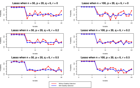
Figure 1: Selection Probabilities for Lasso when $p=20,~{}q=6$

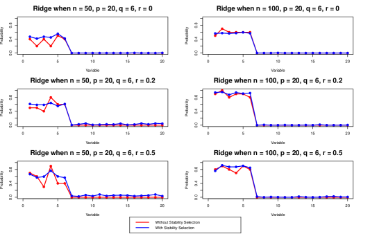
Figure 2: Selection Probabilities for Ridge when $p=20,~{}q=6$

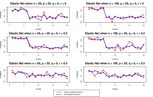
Figure 3: Selection Probabilities for Elastic net when $p=20,~{}q=6$

From Table 1 we see that compared to without stability selection, F+ is smaller when stability selection is applied to the Lasso and elastic net methods and this holds true at all sample sizes and correlation structures. In case of ridge regression, F+ is similar or slightly higher when stability selection is applied as compared to without stability selection. Table 1 also shows that smaller values for F- are obtained when stability selection is applied to ridge regression. In case of the Lasso and elastic net, F- is either slightly higher when stability selection is applied or similar to the values obtained without stability selection when $r=0$ or 0.2. An exception occurs when $r=0.5$ in case of the elastic net where the F- values are lower when stability selection is applied. The selection probability of each variable under the regularization methods with stability selection and without stability selection are shown in Figure 1 for Lasso, in Figure 2 for ridge regression and in Figure 3 for elastic net.

According to these figures the selection probabilities of first six variables are significantly higher than the remaining fourteen variables with the exception of the elastic net for $r=0.5$. This is consistent with our simulated data structure in which the first six variables are designed to have a significant effect on survival time while the remaining variables have no effect. The selection probabilities of the variables remain quite stable when stability selection is applied whereas they tend to fluctuate when there is no stability selection. This is true irrespective of the magnitude of the correlation between variables and sample size. For a conventional choice of the threshold parameter $\pi_{thr}$, use of the stability selection approach ensures that the significant variables are selected with high probability. On the other hand, there is a tendency for false positive errors and false negative errors to occur when stability selection is not used.

2.2 Simulation II: $~{}p=60,~{}n=50$

2.2.1 Setup

We consider 60 variables among which the first 20 variables are assigned $\beta$ coefficients equal to 5 (i.e. $\beta_{j}=5$ for $j\in{1,\cdots,20}$)$(q=20)$ while the remaining are assigned $\beta$ coefficients equal to zero (i.e. $\beta_{j}=0$ for $j\in{21,\cdots,60})$. We generate data sets of size $n=50$ where $X\sim U(0,1)$ with correlation between the components in $X$ being $r=0$, $r=0.2$ or $r=0.5$. This yields the small $n$ large $p$ scenario. All other setting are the same as in Simulation-$I$.

2.2.2 Evaluation

Efficacy of the stability selection approach is evaluated in terms of the probability of selection for each variable and magnitudes of the false positive (F+) and false negative (F-) rates computed over 100 simulated data sets.

2.2.3 Results

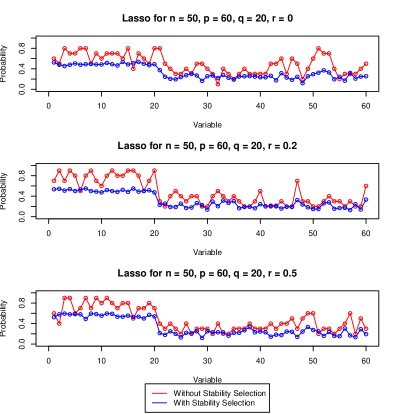
Figure 4: Selection Probabilities for Lasso when $p=60,~{}q=20$

The error rates are given in Table 2. From this table it is seen that for the lasso, F+ is significantly lower when stability selection is applied whereas for the other two methods, F+ is nearly the same with or without stability selection. In general, F- declines for the ridge and elastic net methods when stability selection is applied, however, it increases significantly for the lasso method. The advantage of stability selection in improving variable selection for high dimensional survival data becomes apparent if one observes Figures 4,  5 and  6 for the lasso, ridge and elastic net, respectively. There appears to be large fluctuations in the selection probability of variables irrespective of the level of collinearity between variables when stability selection is not performed. As a result, there is greater error in variable selection as some of the significant variables have low probabilities of selection whereas some of the insignificant variables have relatively large probabilities of selection resulting in large false positive and false negative rates. In contrast, the selection probabilities are stable under stability selection. Furthermore, with the exception of the elastic net at $r=0.5$, the selection probabilities of the significant variables are larger than that of the insignificant variables so that errors are less likely under stability selection. Thus, the results of simulation-$II$ suggest that for a conventional choice of threshold parameter [23], $\pi_{thr}$, a regularization method combined with the stability selection approach can be useful in identifying significant variables in the high dimensional scenario with minimum error.

3 Breast Cancer Data Analysis

We evaluate the stability selection approach for the regularized AFT model using a breast cancer data set that contains the metastasis-free survival times from the study of Veer et al. [30]. Here, a series of 295 patients with primary breast carcinomas were classified as having a gene-expression signature associated with either a poor or a good prognosis. We restrict the study to the 144 patients who had lymph node positive disease and evaluate the predictive value of the gene-expression profile of patients for the 70 genes previously determined by Veer et al. [31] based on a supervised learning method. Five clinical risk factors and 70 gene expression measurements that were found to be prognostic for metastasis-free survival are recorded. The censoring rate is 66%. The variables in the data set are:

• time: metastasis-free follow-up time,

• event: censoring indicator (1 = metastasis or death; 0 = censored),

• diam: diameter of the tumor (two levels),

• N: number of affected lymph nodes (two levels),

• ER: estrogen receptor status (two levels),

• grade: grade of the tumor (three ordered levels),

• age: age of the patient at diagnosis,

• TSPYL5 $\cdots$ C20orf46: gene expression measurements of 70 prognostic genes.

Walschaerts et al. [32] analyzed this breast cancer data set in their study which dealt with stable variable selection methodology. They focussed on new stable variable selection methods based on bootstrap with two survival models–the Cox proportional hazard model and survival trees. Cox model was implemented with two variable selection techniques–bootstrap Lasso selection (BLS) and Bootstrap randomized Lasso selection (BRLS). The survival tree was implemented with the two variable selection techniques–bootstrap node-level stabilization (BNLS) and Random Survival Forests (RSF).

Six covariates were selected by BLS whereas only four were selected by the BRLS procedures in a particular setting for those methods. Six selected covariates by BLS are: PRC1, QSCN6L1, QSCN6L1, IGFBP5.1, ZNF533, COL4A2, Contig63649_RC. Four selected variables by BRLS are: IGFBP5.1, PRC1, ZNF533, QSCN6L1. Tree based procedure RSF and BNLS showed that the most important variable is ZNF533. BNLS selected three other covariates i.e. COL4A2, PRC1 and N and the six most important variables selected by RSF are: ZNF533, PRC1, Age, COL4A2, IGFBP5.1, N. They found that RSF performed the best for prediction because it produced the lowest prediction error rate and selected the most relevant variables to explain the survival durations.

3.1 Lasso, ridge and elastic net with stability selection

Applying stability selection approach on Lasso, we find selection probabilities of all variables. Among them, ten variables have selection probabilities greater than a threshold value of 0.6: Age(0.955), ZNF533(0.845), SCUBE2 (0.8), N(0.75), Grade(0.70), PRC1(0.70), GPR180 (0.675), Contig 63649 RC (0.645), IGFBP5.1(0.615), COL4A2 (0.610). Thus, the results obtained from stability selection for Lasso is close enough to the findings in the study by [32]. Lasso with stability selection selects the same variables as RSF in [32].

Applying stability selection approach on ridge regression, we find seven variables which have selection probabilities greater than 0.6: PRC1(0.805), COL4A2 (0.715), IGFBP5.1 (0.625), GPR180 (0.675), Contig 63649 RC (0.670), ZNF 533 (0.65), PALM2.AKAP2 (0.615). Thus, ridge under stability selection is also able to select seven variables of which five were selected by the RSF [32].

Applying stability selection approach on elastic net, we find ten variables which have selection probabilities greater than 0.6: Age(0.90), N(0.85), ZNF533 (0.84), Grade(0.75), SCUBE2(0.70), PRC1(0.65), IGFBP5.1(0.65), COL4A2 (0.630), Contig63649_RC(0.60), CENPA(0.60). The performance of elastic net under stability selection is also close to the RSF method [32]. Thus, the three regularization methods when combined with stability selection yield the most relevant variables that affect survival. Furthermore, the results are consistent with the findings of [32].

3.2 Lasso, ridge regression and elastic net without stability selection

Applying the AFT regularized by the Lasso on the breast cancer data without stability selection yields fifteen variables: N, Grade, Age, QSCN6L1, SCUBE2, GMPS, GPR180, ZNF533, RTN4RL1, Contig 63649_RC, SLC2A3, HRASLS, PALM2.AKAP2, PRC1, ESM1. Among these variables (COL4A2, IGFBP5.1) were not found significant in the study by [32]. When ridge regression is applied, fifty five variables are found to have high estimated coefficients (e.g. greater than absolute value of one). Although a large number of variables are selected by ridge regression, two important variables (Age, IGFBP5.1) that were found significant in [32] were not selected. When the elastic net was applied, nineteen variables were found to be significant: Diam, N, ER, Grade, Age, QSCN6L1, P5.860F19.3, C16orf61, SCUBE2, ECT2, GSTM3, ZNF533, RTN4RL1, TGFB3, IGFBP5, RTN4RL1, IGFBP5.1, CENPA, NM_004702. However, two variables (COL4A2, PRC1) that were found to be important in the study by [32] using the RSF method were not selected. Thus, regularization of the AFT without stability selection failed to yield a parsimonious model and omitted variables that were found to be important by previous studies.

4 Discussion

Stability in the selection of variables is an important issue when analyzing high dimensional data. Stability selection methods have been evaluated in the context of linear regression and more recently for Cox regression [32]. This study has evaluated whether the stability selection method proposed by [23] can be used to improve variable selection in the AFT model regularized by the lasso, ridge and elastic net methods. These evaluations were made through simulations conducted across different scenarios. False discoveries are a reason for concern in biomedical research since they reduce the reliability of results. In the low dimensional setting ($p<n$), false positive rates were found to be lower when stability selection was applied for most of the cases. Even in the high dimensional scenario ($p>n$), false positive rates decreased in general when stability selection was applied. The selection probabilities were stable for both high and low dimensional survival data when stability selection was applied whereas there were large fluctuations in these probabilities when stability selection was not applied. As a result, some of the significant variables had low selection probabilities while some of the nonsignificant variables had large selection probabilities which increased the likelihood of observing larger numbers of false positives and false negatives. Overall, the advantage of stability selection was apparent across different sample sizes and correlations between variables.

Analysis of the breast cancer data using regularization methods combined with stability selection yielded a parsimonious model containing a small number of variables that were found to be important by other studies as well e.g. [32] and [31]. In contrast, a very large number of variables were selected without stability selection, some of which, were less important and therefore contributed to false positives. On the other hand, some variables found relevant by other studies were not chosen due to their low selection probabilities. Thus, F+ and F- are both likely to be large without stability selection irrespective of the regularization method used. In short, we can conclude that the performance of regularization methods improves when combined with stability selection, particularly, for high–dimensional censored data even when there is collinearity between the covariates leading to a more parsimonious model.

Conflict of interest statement:

The authors have declared no conflict of interest.

Table 1: False positive and False negative rate for three methods with stability selection and without stability selection from 100 simulation runs when $p=20,~{}n=50$ & $100$

Methods	r = 0					r = 0.2					r = 0.5
	n = 50		n = 100			n = 50		n = 100			n = 50		n = 100
	F+	F-	F+	F-		F+	F-	F+	F-		F+	F-	F+	F-
Lasso without Stability	0.42	0.00	0.43	0 .00		0.39	0.01	0.38	0.00		0.34	0.05	0.34	0.00
Lasso with Stability	0.38	0.04	0.40	0.00		0.35	0.05	0.34	0.00		0.30	0.06	0.31	0.02
Ridge without Stability	0.00	0.65	0.00	0.45		0.00	0.43	0.00	0.12		0.00	0.45	0.00	0.19
Ridge with Stability	0.00	0.53	0.00	0.42		0.03	0.40	0.00	0.05		0.05	0.38	0.00	0.14
Elastic Net without Stability	0.34	0.13	0.32	0.05		0.32	0.03	0.32	0.10		0.46	0.40	0.44	0.35
Elastic Net with Stability	0.32	0.18	0.31	0.08		0.31	0.06	0.31	0.09		0.45	0.38	0.42	0.31

Table 2: False positive and False negative rate for three methods with stability selection and without stability selection from 100 simulation runs for $p=60,~{}n=50$

Methods		r = 0			r = 0.2			r = 0.5
		F+	F-		F+	F-		F+	F-
Lasso without Stability Selection		0.41	0.34		0.32	0.23		0.34	0.26
Lasso with Stability Selection		0.24	0.50		0.21	0.48		0.21	0.44
Ridge without Stability Selection		0.00	0.88		0.00	0.69		0.00	0.67
Ridge with Stability Selection		0.03	0.85		0.05	0.66		0.06	0.57
Elastic without Stability Selection		0.41	0.31		0.44	0.39		0.48	0.45
Elastic with Stability Selection		0.41	0.32		0.43	0.38		0.47	0.40

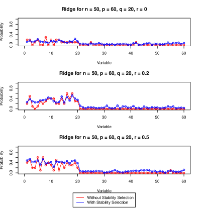
Figure 5: Selection Probabilities for Ridge when $p=60,~{}q=20$

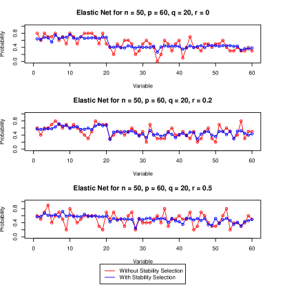
Figure 6: Selection Probabilities for Elastic Net when $p=60,~{}q=20$

References

- [1] Sauerbrei W, Schumacher M. A bootstrap resampling procedure for model building: Application to the cox regression model. Statistics in Medicine 1992; 11:2093–2109.
- [2] Faraggi D, Simon R. Bayesian variable selection method for censored survival data. Biometrics 1998; 54(4):1475–85.
- [3] Ibrahim CMH J G, Maceachern SN. Bayesian variable selection for proportional hazards models. Canadian Journal of Statistics 1999; 27(4):701–17.
- [4] Tibshirani R. Regression shrinkage and selection via the lasso. Journal of the Royal Statistical Society. Series B (Methodological) 1996; :267–288.
- [5] Hoerl AE, Kennard RW. Ridge regression: applications to nonorthogonal problems. Technometrics 1970; 12(1):69–82.
- [6] Efron B, Hastie T, Johnstone I, Tibshirani R, et al.. Least angle regression. The Annals of statistics 2004; 32(2):407–499.
- [7] Zou H, Hastie T. Regularization and variable selection via the elastic net. Journal of the Royal Statistical Society: Series B (Statistical Methodology) 2005; 67(2):301–320.
- [8] Candes E, Tao T. The dantzig selector: Statistical estimation when is much larger than . The Annals of Statistics 2007; :2313–2351.
- [9] James GM, Radchenko P. A generalized dantzig selector with shrinkage tuning. Biometrika 2009; 96(2):323–337.
- [10] Leng C LY, G W. A note on the LASSO and related procedures in model selection. Statistics Sinica 2006; 16:1273–1284.
- [11] Tibshirani R. The lasso method for variable selection in the cox model. Statistics in medicine 1997; 16(4):385–395.
- [12] Gui J, Li H. Penalized Cox regression analysis in the highdimensional and low-sample size settings, with applications to microarray gene expression data. Bioinformatics 2005; 21:3001–3008.
- [13] Tern s RF N, Michielsa S. Empirical extensions of the LASSO penalty to reduce the false discovery rate in high dimensional cox regression models. Statistics in Medicine 2016; :DOI: 10.1002/sim.6927.
- [14] Fan J, Li R. Variable selection for Cox s proportional hazards model and frailty model. The Annals of Statistics 2002; 30:74–99.
- [15] Zhang HH, Lu W. Adaptive lasso for Cox s proportional hazards model. Biometrika 2007; 94:691–703.
- [16] Li H, Luan Y. Kernel Cox regression models for linking gene expression profiles to censored survival data. Pacific Symposium of Biocomputing 2003; 8:65–76.
- [17] Gui J, Li H. Threshold gradient descent method for censored data regression, with applications in pharmacogenomics. Pacific Symposium on Biocomputing 2005; 10:272–283.
- [18] Wei L. The accelerated failure time model: a useful alternative to the cox regression model in survival analysis. Statistics in medicine 1992; 11(14-15):1871–1879.
- [19] Swindell w. Accelerated failure time models provide a useful statistical framework for aging research. Experimental gerontology 2009; 44(3):190–200.
- [20] Huang MS J, Xie H. Regularized estimation in the accelerated failure time model with high-dimensional covariates. Biometrics 2006; 62:813–820.
- [21] Huang J, Ma S. Variable selection in the accelerated failure time model via the bridge method. Lifetime data analysis 2010; 16:176–195.
- [22] Wang NBZJ S, Beer D. Doubly penalized buckley-james method for survival data with high-dimensional covariates. Biometrics 2008; 64:132–140.
- [23] Meinshausen N, Bühlmann P. Stability selection. Journal of the Royal Statistical Society: Series B (Statistical Methodology) 2010; 72(4):417–473.
- [24] Stute W. Consistent estimation under random censorship when covariables are present. Journal of Multivariate Analysis 1993; 45(1):89–103.
- [25] Kalbfleisch JD, Prentice RL. The statistical analysis of failure time data. John Wiley & Sons, 2011.
- [26] Huang J, Ma S, Xie H. Regularized estimation in the accelerated failure time model with high-dimensional covariates. Biometrics 2006; 62(3):813–820.
- [27] Khan MHR. Variable selection and estimation procedures for high-dimensional survival data. Ph.D. Thesis, Department of Statistics, University of Warwick, UK 2013; .
- [28] Khan MHR, Shaw JEH. Variable selection for survival data with a class of adaptive elastic net techniques. Statistics and Computing 2016; 26(3):725–741.
- [29] Khan MHR, Shaw JEH. Variable selection with the modified buckley-james method and the dantzig selector for high-dimensional survival data. CRiSM Working Paper 2014; (University of Warwick, UK. No. 14-28).
- [30] Van De Vijver MJ, He YD, van’t Veer LJ, Dai H, Hart AA, Voskuil DW, Schreiber GJ, Peterse JL, Roberts C, Marton MJ, et al.. A gene-expression signature as a predictor of survival in breast cancer. New England Journal of Medicine 2002; 347(25):1999–2009.
- [31] van’t Veer LJ, Dai H, Van De Vijver MJ, He YD, Hart AA, Mao M, Peterse HL, van der Kooy K, Marton MJ, Witteveen AT, et al.. Gene expression profiling predicts clinical outcome of breast cancer. nature 2002; 415(6871):530–536.
- [32] Walschaerts M, Leconte E, Besse P. Stable variable selection for right censored data: comparison of methods. arXiv preprint arXiv:1203.4928 2012; .