The turbulent diffusion of toroidal magnetic flux as inferred from properties of the sunspot butterfly diagram

Abstract

Context. In order to match observed properties of the solar cycle, flux-transport dynamo models require the toroidal magnetic flux to be stored in a region of low magnetic diffusivity, typically located at or below the bottom of the convection zone.

Aims. We infer the turbulent magnetic diffusivity affecting the toroidal field on the basis of empirical data.

Methods. We consider the time evolution of mean latitude and width of the activity belts of solar cycles 12–23 and their dependence on cycle strength. We interpret the decline phase of the cycles as a diffusion process.

Results. The activity level of a given cycle begins to decline when the centers of its equatorward propagating activity belts come within their width (at half maximum) from the equator. This happens earlier for stronger cycles because their activity belts are wider. From that moment on, the activity and the belt width decrease in the same manner for all cycles, independent of their maximum activity level. In terms of diffusive cancellation of opposite-polarity toroidal flux across the equator, we infer the turbulent diffusivity experienced by the toroidal field, wherever it is located, to be in the range 150–450 km²s^-1. Strong diffusive latitudinal spreading of the toroidal flux underneath the activity belts can be inhibited by an inflow towards the toroidal field bands in the convection zone with a magnitude of several meters per second.

Conclusions. The inferred value of the turbulent magnetic diffusivity affecting the toroidal field agrees, to order of magnitude, with estimates based on mixing-length models for the solar convection zone. This is at variance with the requirement of flux-transport dynamo models. The inflows required to keep the toroidal field bands together before they approach the equator are similar to the inflows towards the activity belts observed with local helioseismology.

1 Introduction

Our understanding of the solar dynamo is based on theory, helioseismology, and the observational clues that we can derive from the emergence of the magnetic flux through the solar surface and its subsequent evolution. A well studied theoretical model is the Flux-Transport Dynamo (FTD), which explains the equatorward migration of the activity belts in terms of advective transport of toroidal flux by assuming a deep return flow of the observed near-surface poleward meridional flow. In order for this mechanism to work, the turbulent magnetic diffusivity affecting the toroidal field needs to be low enough to be overcome by the flow. Since simple estimates of the turbulent magnetic diffusivity in the convection zone based on the mixing length model give high values of the order of $1000$ km²s${}^{-1},$ most FTD models therefore assume that the toroidal flux is generated mainly by radial differential rotation associated with the tachocline and stored in a region of much lower magnetic diffusivity at or below the bottom of the convection zone (for reviews, see, e.g. Dikpati & Gilman, 2009; Charbonneau, 2010, 2014; Karak et al., 2014). Low diffusivity, possibly together with downward convective pumping (e.g. Jiang et al., 2013; Lawson et al., 2015), also prevents rapid loss of toroidal flux by radial diffusion (Zita, 2010). Alternatively, it has been suggested that the required low values of the magnetic diffusivity affecting the toroidal field could be provided within the convection zone through diffusivity quenching by a sufficiently strong magnetic field (e.g. Muñoz-Jaramillo et al., 2011). In any case, the toroidal flux needs to be associated by a magnetic diffusivity that is orders of magnitude lower than the estimates for the convection zone based on mixing-length models.

In this paper, we use observations to infer the turbulent magnetic diffusivity, $\eta_{\mathrm{t}}$, affecting the toroidal flux bands that provide the source of the magnetic flux emerging to form sunspot groups. We base our analysis on the properties of the time-latitude diagram of sunspot emergence (butterfly diagram) derived from the RGO/SOON sunspot record for solar cycles 12–23. We find that all cycles decline in the same manner once the centers of their activity belts have approached the solar equator to within their width at half maximum (Section 2). Interpreting this result in terms of toroidal flux diffusing across the equator and cancelling with opposite-polarity flux, we determine a range of values for $\eta_{\mathrm{t}}$ that is within an order of magnitude with the mixing-length result for the convection zone (Section 3). This is in contrast to the requirement of FTD models that the toroidal field should be affected by a much lower magnetic diffusivity.

The high value of $\eta_{\mathrm{t}}$ would lead to severe spreading of the activity belts before they have propagated into the vicinity of equator, contrary to what is observed. Such spreading could be prevented by a latitudinal inflow towards the toroidal field bands. We estimate the structure and amplitude of such a flow in Section 4. It turns out that the properties of the inferred flow are similar to those of the observed shallow inflows towards the activity belts (Gizon et al., 2001; Gizon, 2004; Zhao & Kosovichev, 2004).

2 Properties of the butterfly diagram

Figure 1 shows the emergence rate of sunspot groups as a function of time and latitude, based on the RGO/SOON sunspot group records. We constructed this ‘butterfly diagram’ by binning the sunspot groups in yearly and 1-degree bins, considering each group at the time of its maximum area.

Figure 1: Time-latitude diagram (butterfly diagram) of the rate of sunspot group emergence based on the RGO/SOON data sets.

Similar to the analysis of Ivanov et al. (2011), we determined yearly values of the central latitude and the full width at half maximum of the butterfly wings, i.e., the migrating activity belts. We fitted Gaussians to the latitudinal profiles in both hemispheres using the curve_fit routine of NumPy (version 1.8.1). Examples of the original profiles and the Gaussian fits for the years 1903 (during the early phase of the weak cycle 17) and the year 1957 (during the early phase of the strong cycle 19) are shown in the left panel of Figure 2. We also fitted the emergence rates in both hemispheres together (as a function of unsigned latitude); the corresponding fit is shown in the right hand panel. In most of the following we will show the results for the fits based on the unsigned latitude (i.e., considering both hemispheres together) because the noise is lower. The main deviation from the Gaussian shape occurs near the equator, where fewer sunspots are observed than indicated by the Gaussian fits. Such an asymmetry is expected if the two activity belts (or rather the underlying oppositely directed toroidal flux systems) interact destructively and cancel each other across the equator.

Figure 2: Latitudinal cuts through the butterfly diagram shown in Fig. 1 for the years 1903 (during the weak cycle 14, solid red curve) and 1957 (during the strong cycle 19, solid black curve). In the left panel, the dashed (dash-dotted) curve represents a Gaussian fit to the number of spot groups in the southern (northern) hemisphere. In the right panel, the two hemispheres were fitted together with a single Gaussian.

We determine three parameters describing the evolution of the activity belt: amplitude $A(t)$, central latitude $\lambda_{c}(t)$, and its full width at half maximum, $w(t)$. In addition, we consider the yearly international sunspot number, $S(t)$ (version 2.0 SILSO World Data Center, 1874-2015), all for cycles 12 through 23. Because cycles overlap in time by a few years, which is not accounted for in our Gaussian fitting, we follow Solanki et al. (2008) and consider the parameters only from years $2$ to $9$ during each cycle. Because we are interested in the relationship between activity and the latitudinal distribution (described by $\lambda_{c}(t)$ and $w(t)$), we can choose to consider either $S(t)$ and $A(t)\times w(t)$ as measure of the activity level. We have tested both choices and found the results to be similar. Here we present the results based on $S(t)$ because as a measure of activity it has been well studied and calibrated (Clette et al., 2014). In the following we therefore consider the relation between the three quantities $\lambda_{c}(t)$, $w(t)$, and $S(t)$, which describe the evolution of the activity belts during the cycles covered by the data.

Figure 3 shows the sunspot number, $S(t)$, as a function of the central latitude of the activity belt, $\lambda_{c}(t)$, separately for cycles 12 to 23. This plot is similar to Figure 6d of Ivanov & Miletsky (2014), except that we use the central latitude obtained from the fits for each year while they use an empirically derived model of the central latitude. This difference has no substantial impact. We see that each cycle begins with a different activity level at high latitude. As the activity belt propagates towards the equator, the sunspot number at first increases and then decreases sharply. The latitude at which the sunspot number begins to decrease depends on the strength of the cycle, with stronger cycles beginning to decline already when their activity belts are at higher latitudes. Because $\lambda_{c}$ moves towards the equator in the same way for all cycles (Waldmeier, 1955; Hathaway, 2011), the decrease at high latitudes for stronger cycles is equivalent to a decrease earlier in the cycle than for weaker cycles. The fact that strong cycles begin to decline earlier is known as the Waldmeier effect. After they begin to decline, all the cycles show a similar sunspot number as a function of their mean unsigned latitude. The straight black line in Figure 3 given by $S=25\lambda_{c}-200$ gives a rough approximation of this common declining phase.

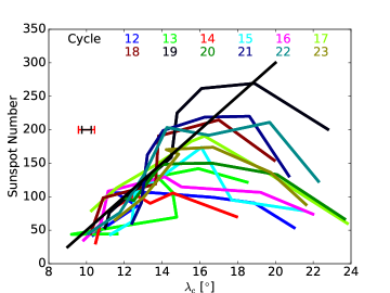
Figure 3: Yearly International Sunspot Number $S$ (SILSO World Data Center, 1874-2015) for cycles 12 to 23 as a function of the mean unsigned latitude of the sunspots each year. The line colors indicate the different cycles. The thin black curve is an approximate fit to the declining phase: $S=25\lambda_{c}-200$. Error bars on the left side indicate standard deviations of $\lambda_{c}$ from the Gaussian fitting procedure carried out for each year: the maximum value is shown in red while the mean over all years is given in black.

Next we consider the relationship between the full width at half maximum, $w(t)$, and the central latitude, $\lambda_{c}(t)$, of the activity belts for cycles 12 to 23, which is shown in Figure 4. The belt width as a function of mean unsigned latitude behaves in analogy to the sunspot number shown in the previous figure: stronger cycles begin with a high $w$ that starts to decrease at higher latitudes than during weaker cycles. In their declining phases (at low latitudes), all cycles show a similar decrease of $w$. The common behavior in the declining phase can be approximated by the relation $w=1.1\lambda_{c}$.

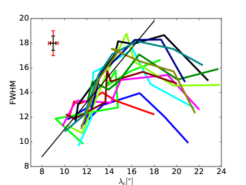
Figure 4: Full width at half maximum ($w$) of the activity belts as a function of the mean unsigned latitude of the sunspots each year. Different colors represent different cycles as in Fig. 3. The thin black curve is an approximate fit to the declining phase: $\mbox{$w$}=1.1\lambda_{c}$. Error bars on the top left indicate standard deviations of $\lambda_{c}$ and $w$, respectively, from the Gaussian fit procedure carried out for each year: maximum values are shown in red while the mean values over all years are given in black.

An important point for the interpretation of the results is that the decline of activity once the sunspot belts have approached the equator to within their width affects all latitudes within the belts in the same way; it is a universal decline, not just a decrease on its equatorward side. This is illustrated in Fig. 5, which shows the evolution of the activity belts for the strongest cycles (numbers 19 and 21) and the weakest cycles (numbers 14 and 16) in the data set. Relative to the year when $\lambda_{c}$ was between $13^{\circ}$ and $15^{\circ}$ latitude (year zero, black lines), the plots show the latitudinal distribution of sunspot activity in the two preceding and up to five subsequent years. For the strong cycles, the decline begins at year zero while for the weak cycles the belts continue to migrate equatorwards for another two years with no significant change of amplitude. The activity profiles for the following two years then show an overall decrease: activity declines at all latitudes of the activity belt while the shape stays roughly Gaussian.

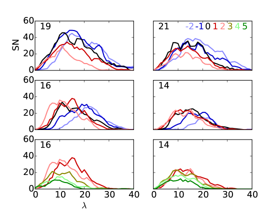
Figure 5: Latitudinal distribution of sunspots for several years during cycles 19 (upper left), 21 (upper right), 16 (middle and lower left) and 14 (middle and lower right). The black curves are for the years when the mean latitude of the sunspots was between $13^{\circ}$ and $15^{\circ}$. The colours of the other curves indicate the year relative to this reference year (see legend in the top left panel). The curves were smoothed with a 3 degree box-car filter. The late phases of cycles 14 and 16 are shown separately (bottom panels) in order to avoid too strong crowding of lines.

At this point, we have seen that all cycles decline in a very similar way: the activity belts propagate towards the equator at the same rate, and both their amplitude and width can be approximated by simple functions of their latitudinal distance from the equator. Cycles grow at different rates, with stronger cycles beginning to decline earlier (the Waldmeier effect). But once they begin to decline, cycles all decline in a similar way and the activity decreases over the whole width of the activity belts. We discuss the implications of these results in the next section.

3 Interpretation and estimate of $\eta_{\mathrm{t}}$

The basic result obtained in the previous section is that all cycles decline in the same way. Figs. 3–5 indicate that the activity belts propagate towards the equator showing increasing or approximately constant levels of activity until their distance from the equator becomes about equal to their width. Thereafter the activity strongly decreases across the whole latitude range covered by the belts. Stronger cycles begin with a larger width of their activity belts and thus start to decline earlier than weaker cycles. Once they begin to decline, all cycles follow the same pattern in terms of amplitude and latitudinal distribution. These properties suggest an interpretation of the declining phase in terms of cross-equator diffusion and cancellation of toroidal magnetic flux. We consider this possibility by a quantitative analysis, which provides an estimate of the magnitude of the relevant magnetic diffusivity.

For our analysis, we use radians as unit for $\lambda$ and $w(t)$. We consider the distribution of sunspots as a function of latitude and time, $N(\lambda,t)$, assuming that the activity belts in both hemispheres are symmetric with respect to the equator. We model this quantity as a Gaussian with full width at half maximum given by $w(t)$, centered at $\lambda_{c}$ and with a total area given by the sunspot number $S/2$, viz.

$$N(\lambda,t)=\frac{S(t)}{2\sigma\sqrt{2\pi}}\exp{\left(-\frac{(\lambda-\lambda_{c})^{2}}{2\sigma^{2}}\right)}$$ (1)

where $\sigma(t)=w(t)/\sqrt{8\ln 2}$.

We assume that the latitudinal profiles of the activity belts represent those of the underlying bands of toroidal magnetic flux from which the bipolar magnetic regions and sunspots emerge. This appears to be a reasonable assumption since the activity belts do not overlap and even at low latitudes it is uncommon to see sunspot groups not obeying Hale’s polarity rules. If we assume further that the emerging flux (represented by the sunspot number) is proportional to the radially integrated toroidal flux density at each latitude, we obtain

$$\int_{0.7R_{\odot}}^{R_{\odot}}rB_{\phi}(r,\lambda,t)\mathrm{d}r=\alpha N(\lambda,t),$$ (2)

where $B_{\phi}(r,\lambda,t)$ is the longitudinally averaged azimuthal component of the magnetic field, $\alpha$ is a constant of proportionality (which drops out of the final result), and $R_{\odot}$ is the solar radius.

We interpret the observational results illustrated in Figs. 3–5 in terms of diffusive cancellation of the oppositely oriented toroidal flux bands across the equator. This interpretation is motivated by the above result that the decline in activity each cycle begins only when the activity belts come within their width of the equator, but from then on affects the whole activity belt. This behavior suggests that the loss of toroidal flux across the equator dominates over the losses due to cancellation at the axis of rotation as well as due to downward pumping of flux toward stable layers near the bottom of the convection zone. We consider the rate, $D_{\mathrm{eq}}$, at which toroidal flux in the northern hemisphere is transported across the equatorial plane by diffusion. Applying Stokes’ theorem to the integrated toroidal flux over a hemisphere yields

$$D_{\mathrm{eq}}=\int_{0.7R_{\odot}}^{R_{\odot}}\left.\frac{\eta_{\mathrm{t}}(r)}{r}\frac{\partial B_{\phi}(r,\lambda,t)}{\partial\lambda}\right|_{\lambda=0}dr,$$ (3)

where $\eta_{\mathrm{t}}(r)$ is the turbulent magnetic diffusivity. Since the depth-dependence of the toroidal field (i.e., the storage location of the toroidal flux) is unknown, we rewrite Eq. (3) in the form

$$D_{\mathrm{eq}}=\left(\frac{\eta}{R^{2}}\right)_{\mathrm{e}}\frac{\partial}{\partial\lambda}\left(\left.\int_{0.7R_{\odot}}^{R_{\odot}}rB_{\phi}(r,\lambda,t)dr\right)\right|_{\lambda=0}$$ (4)

where $(\eta/R^{2})_{\mathrm{e}}^{-1}$ is an effective diffusion time of the toroidal flux. If the flux is stored in a narrow radial layer around $r=R_{0}$, then $(\eta/R^{2})_{\mathrm{e}}=\eta_{\mathrm{t}}(R_{0})/R_{0}^{2}$ and the relevant turbulent magnetic diffusivity affecting the toroidal field is given by $\eta_{\mathrm{t}}(R_{0})$. For more general distributions, $(\eta/R^{2})_{\mathrm{e}}$ represents the effective quantity describing the diffusion of the toroidal flux. Using Eq. (2), we obtain

$$D_{\mathrm{eq}}=\left(\frac{\eta}{R^{2}}\right)_{\mathrm{e}}\alpha\left.\frac{\partial N}{\partial\lambda}\right|_{\lambda=0}$$ (5)

and substituting Eq. (1) we find

$$D_{\mathrm{eq}}=\left(\frac{\eta}{R^{2}}\right)_{\mathrm{e}}\alpha\frac{\lambda_{c}S}{2\sigma^{3}\sqrt{2\pi}}\exp{\frac{-\lambda_{c}^{2}}{2\sigma^{2}}}.$$ (6)

for the rate at which the northern hemisphere loses toroidal flux by turbulent diffusion over the equator. Since opposite-polarity flux from the southern hemisphere diffuses into the northern hemisphere at the same rate, $D_{\mathrm{eq}}$ is actually half the rate at which the toroidal flux in the northern hemisphere decreases. Therefore we have

$$D_{\mathrm{eq}} = \frac{1}{2}\frac{d}{dt}\int_{0}^{\pi/2}\int_{0.7R_{\odot}}^{R_{\odot}}rB_{\phi}(r,\lambda,t)\mathrm{d}rd\lambda$$ (7)

$$= \frac{\alpha}{2}\frac{d}{dt}\int_{0}^{\pi/2}N(\lambda,t)d\lambda$$

$$= \frac{\alpha}{4}\frac{dS}{dt}.$$

Equating Eqs. (6) and (7) yields

$$\frac{dS}{dt}=4\left(\frac{\eta}{R^{2}}\right)_{\mathrm{e}}\frac{\lambda_{c}S}{2\sigma^{3}\sqrt{2\pi}}\exp{\frac{-\lambda_{c}^{2}}{2\sigma^{2}}}.$$ (8)

To model the declining phase, we use the empirical relations obtained in Sec. 2, namely

$$\lambda_{c} = (S+200)/25\times\pi/180$$ (9)

$$= 7\times 10^{-4}(S+200)$$

from Figure 3 and

$$\sigma = w/\sqrt{8\ln{2}}=0.47\lambda_{c}$$ (10)

$$= 3.3\times 10^{-4}(S+200)$$

from Figure 4. Equation (8) then is a nonlinear ODE, which describes the evolution of the sunspot number during the declining phase of a cycle. We solve this ODE numerically. Figure 6 shows the observed decrease in $S$ as a function of time (counted from activity minimum) for each cycle. The thick black curves show estimates for the evolution of $S(t)$ based on Eq. (8) corresponding to two values of $(\eta/R^{2})_{\mathrm{e}}R_{\odot}^{2}$: $450$ km²s^-1 (solid black curve) and $300$ km²s^-1 (dashed black curve). Since $1\leq{R_{\odot}^{2}}/{R^{2}}\la 2$, we obtain values in the range of $150$ km²s^-1 to $450$ km²s^-1 for the effective turbulent diffusivity affecting the toroidal flux bands, with most of the uncertainty being due to the uncertainty in the depth at which the toroidal flux is located.

One may imagine alternative explanations of the observed evolution of the activity belts discussed in Sec. 2, which would allow the toroidal field to be stored in a low-diffusivity environment somewhere below the convection zone proper. One possibility would be magnetoshear instabilities in the tachocline (e.g. Cally et al., 2003; Gilman et al., 2007). However, these instabilities are not restricted to low latitudes and also would require a very peculiar nonlinear development in order to reproduce the uniform decline of activity throughout the whole activity belt and its onset depending on the width of the belt. The same problem is faced when assuming a field-dependent low-latitude upflow part of the meridional circulation: it needs to be of a very contrived field-dependent form to be able to reproduce the observed evolution of the activity belts, i.e., mimick a diffusion process.

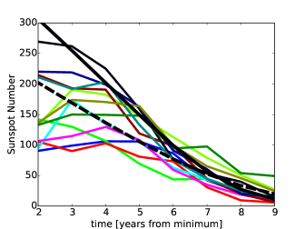
Figure 6: Sunspot Number as a function of time of minimum activity. Different colors represent different cycles as in Fig. 3.

4 Inflows maintaining the activity belts

The high value for the turbulent magnetic diffusivity obtained here raises a problem. Our estimated range of diffusivities, 150–450 km²s^-1, corresponds to 5.7²–9.8² deg²year^-1. If diffusion were the only process operating, then even with the lower diffusivity an initial Gaussian distribution with a FWHM of $14^{\circ}$ degrees would increase its width by about $9.4^{\circ}$ after only one year. This is inconsistent with the observed development of the activity belts during the rising phase of a cycle (cf. Fig. 4), which show an increase of their width by only roughly 2–3^∘ per year. To restrict the spread of the wings to $3^{\circ}$ or less would require the diffusivity to be less than 40 km²/s^-1. Higher values of the diffusivity therefore require the existence of an antidiffusive effect to counter too strong spreading of the activity belts. One possibility is to suppose that the toroidal field is affected by a latitudinal flow (inflow) towards the activity belt such that diffusive spreading is (partially) balanced by advection. Here we consider the simple kinematic problem with the aim of estimating the properties of an inflow that would balance the diffusive spreading.

To estimate the geometry and amplitude of such a flow field, we consider the induction equation for the azimuthally averaged magnetic field, ${\bf B}$,

$$\frac{\partial{\bf B}}{\partial t}=\nabla\times({\bf U}\times{\bf B})-\nabla\times\eta_{\mathrm{t}}\nabla\times{\bf B}.$$ (11)

The rate at which the activity belts propagate towards the equator is about 1–2 degrees per year, while the expected diffusive spreading is substantially higher. Therefore we can make the approximation that the diffusion is balanced by the advective transport, i.e.

$$\nabla\times({\bf U}\times{\bf B})=\nabla\times\eta_{\mathrm{t}}\nabla\times{\bf B}.$$ (12)

Integration yields

$${\bf U}\times{\bf B}=\eta_{\mathrm{t}}\nabla\times{\bf B},$$ (13)

where we have set the arbitrary scalar potential to zero. The radial component of Eq. (13) reads

$$U_{\lambda}B_{\phi}=\frac{\eta_{\mathrm{t}}}{r\sin(\lambda)}\frac{\partial\sin(\lambda)B_{\phi}}{\partial\lambda}\,.$$ (14)

On the left-hand side of this equation, we have neglected the term $-U_{\phi}B_{\lambda}$, which describes the generation of toroidal field by differential rotation. This is justified since we show in Appendix A that the rate of flux change due to differential rotation in the low latitudes covers at most 10% of the required value derived from the observed butterfly diagram of sunspot emergence.

Similar to the determination of the effective diffusion time, $(\eta/R^{2})_{\mathrm{e}}^{-1}$, in Sec. 3 we derive an effective advection time, $(U_{\lambda}/R)_{\mathrm{e}}^{-1}$, of the toroidal flux owing to latitudinal inflows. Integrating Eq. (14) over radius and introducing the effective time scales we obtain

$$(U_{\lambda}/R)_{\mathrm{e}}\int_{0.7R_{\odot}}^{R_{\odot}} r B_{\phi}(r,\lambda,t)\mathrm{d}r=$$ (15)

$$= \frac{(\eta/R^{2})_{\mathrm{e}}}{\sin\lambda}\frac{\partial}{\partial\lambda}\left(\sin\lambda\int_{0.7R_{\odot}}^{R_{\odot}}rB_{\phi}(r,\lambda,t)\mathrm{d}r\right)\,.$$

Using Eq. (2) then yields

$$(U_{\lambda}/R)_{\mathrm{e}}=\frac{(\eta/R^{2})_{\mathrm{e}}}{N(\lambda,t)\sin\lambda}\frac{\partial}{\partial\lambda}\left[N(\lambda,t)\sin\lambda)\right]\,,$$ (16)

connecting the effective inflow with the time-latitude development of the sunspot emergence rate $N(\lambda,t)$ shown in Figure 1. If the toroidal flux is stored in a narrow radial layer around $r=R_{0}$, then $(U_{\lambda}/R)_{\mathrm{e}}=U_{\lambda}(R_{0})/R_{0}$ and the relevant inflow velocity is given by $U_{\lambda}(R_{0})$.

We evaluated Eq. (16) on the basis of an avererage butterfly diagram in order to reduce the noise. All cycles in our dataset were aligned in time with respect to the year during which the mean latitude of the sunspot groups in each wing is closest to 15^∘. The choice of 15^∘ is somewhat arbitrary, but all cycles showed a reasonable number of sunspots near this latitude and the results are not strongly sensitive to this choice. The average butterfly diagram constructed in this way is shown in Figure 7. We used the data for this average cycle and Eq. (16) together with Eq. (2) to obtain $(U_{\lambda}/R)_{\mathrm{e}}R_{\odot}$ for an intermediate value of the magnetic diffusivity given by $(\eta/R^{2})_{\mathrm{e}}R_{\odot}^{2}=300\,$km²s^-1. The result is shown in Figure 8. Considering the ranges for $(\eta/R^{2})_{\mathrm{e}}R_{\odot}^{2}=150\dots 450\,$km²s^-1 and $R/R_{\odot}=0.7\dots 1$, the corresponding amplitudes of $U_{\lambda}$ become between 65% lower ($\simeq 3\,$m s^-1) and 50% higher ($\simeq 12\,$m s^-1).

Note that we estimate $U_{\lambda}$ under the assumption that advection exactly balances the outward diffusion. This is no longer valid near the equator in the declining phase of a cycle, when the activity belts approach each other. Since the inflows probably extend beyond the activity belts, the overlapping between the flow systems of the two hemispheres reduces the inflows and thus allows for cross-equatorial diffusion of toroidal flux. The high velocities near the equator seen in Figure 8 should therefore not be considered as realistic.

The inflows derived here are similar in both extent and amplitude to the actually observed shallow inflows into the active region latitudes (Gizon et al., 2001; Gizon, 2004; Zhao & Kosovichev, 2004). Furthermore, Komm et al. (2015) showed that the inflows are part of the extended solar cycle, beginning at mid latitudes (about 40 degrees). The inflows then propagate equatorward together with the activity belts. The extension in depth of these flows is unclear at the moment. Liang & Chou (2015) report that the helioseismic signature of the inflows is present down to 0.88–0.93 $R_{\odot}$, and partly present at depths from 0.75–0.88 $R_{\odot}$. On the other hand, Gizon & Rempel (2008) report a return flow at a depth of about 60 Mm ($\simeq 0.91R_{\odot}$). Such rather shallow inflows could result from cooling associated with the excess brightness of facular areas (Spruit, 2003). Deep inflows could be driven by thermal perturbations caused by toroidal field amplification near the base of the convection zone (Rempel, 2003). In fact, there are helioseismic indications of cycle-related changes of the sound speed in this region (Baldner & Basu, 2008).

Since the inflows probably extend only over a limited depth range in the convection zone, we expect that part of the toroidal flux is spread over the convection zone by radial turbulent diffusion and an outward return flow. The effect of a deep return flow (in case of an inflow confined to the upper convection zone) is negligible since, owing to mass conservation and the strong increase of density with depth, its speed is much lower than that of the inflow. Radial turbulent diffusion cannot be neglected in this case, but the solution of a simple 2D advection-diffusion problem shows that still a substantial part of the toroidal flux is kept confined in the convergence zone of the inflows.

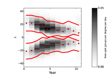
Figure 7: The average activity belts, based on aligning the butterfly wings shown in Figure 1. The alignment was based on the year in which the average latitude of the wings is closest to 15 degrees. The red dots show the latitudes at which the activity belts are centered each year, and the red lines show the central latitude $\pm 12^{\circ}$.

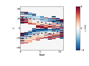
Figure 8: The velocity required to prevent the activity belts from diffusing in latitude. The velocity is only shown in the latitudes within the red lines shown in Figure 7.

5 Conclusion

Solar cycles begin to decline when the distance of the center of the activity belts from the equator becomes about equal to their width (at half maximum). From this time onward, activity decreases across the whole latitude range covered by the belts and all cycles decline in the same way. Stronger cycles show wider activity belts and thus start to decline earlier than weaker cycles. This is the essence of the Waldmeier effect (Waldmeier, 1955).

We interpret this result in terms of oppositely directed toroidal flux bands in each hemisphere that diffuse and cancel across the equator. The observational results are consistent with a diffusion process with effective value of the turbulent diffusivity acting on the toroidal magnetic field in the range $150$ km²s^-1 to $450$ km²s^-1. This is consistent (to order of magnitude) with the mixing length theory estimate, but inconsistent with the much lower values required by flux transport dynamos. Other interpretations of the observations in terms of magnetoshear instability or magnetic-field dependent upflows would require rather contrived properties of these processes, for which there is no evidence.

The flow field required to maintain the butterfly wings against the effects of diffusion is an inflow of a few meters per second, centered on the activity belts. Its spatial extent is at least $12^{\circ}$ on both sides of the activity belt. Inflows with similar properties have been observed in the upper part of the convection zone, but may extend also to deeper layers.

Appendix A Generation of toroidal flux by differential rotation

In order to estimate the effect of low-latitude generation of toroidal flux by differential rotation in the declining phase of an activity cycle, we consider the time derivative of the axisymmetric toroidal magnetic flux, $\int_{R_{T}}^{R_{\odot}}B_{\phi}r\mathrm{d}r$, radially integrated from the top of the tachocline, $R_{T}$, to the surface, $R_{\odot}$, as a function of latitude. This puts aside the question where the toroidal flux is located in radius, but still requires us to make some assumptions on the internal structure of the magnetic field. Firstly, we assume that turbulent/convective pumping expels the horizontal components of the field from the near-surface shear layer (NSSL), so that the field there becomes purely radial. Secondly, we assume that the radial shear is zero between the NSSL and the top of the tachocline, and, thirdly, we assume that the magnetic field does not penetrate into the tachocline. Owing to the prolate shape of the tachocline (e.g. Antia & Basu 2011), the last assumption is somewhat questionable in higher latitudes, but here we are mainly interested in the flux generation in the low-latitude activity belts, where the main part of the tachocline is located below the convection zone. In addition, toroidal flux generation in the tachocline faces the problem of maintaining the required radial shear in the presence of a substantial Lorentz force and weak (or even absent) convection (Gilman & Rempel 2005; Spruit 2011).

In what follows we use a proper right-handed system of spherical coordinates, $(r,\theta,\phi)$. The contribution of differential rotation, $U_{\phi}=\Omega(r,\theta)\,r\sin\theta$, to the evolution of the azimuthally averaged toroidal field, $B_{\phi}$, is given by

$$\frac{\partial B_{\phi}}{\partial t} = \frac{1}{r}\left[\frac{\partial(rU_{\phi}B_{r})}{\partial r}+\frac{\partial(U_{\phi}B_{\theta})}{\partial\theta}\right]$$ (17)

$$= \frac{1}{r}\left[\frac{\partial}{\partial r}(\Omega\,r^{2}\sin\theta\,B_{r})+\frac{\partial}{\partial\theta}(\Omega\,r\sin\theta\,B_{\theta})\right]\,.$$

Integrating over radius yields

$$\frac{\partial}{\partial t}\int_{R_{T}}^{R_{\odot}}B_{\phi}r\,\mathrm{d}r= \int_{R_{T}}^{R_{\odot}} \sin\theta\,\frac{\partial(\Omega r^{2}B_{r})}{\partial r}\,\mathrm{d}r$$ (18)

$$+ \frac{\partial}{\partial\theta}\int_{R_{T}}^{R_{\odot}}\Omega\sin\theta\,B_{\theta}r\,\mathrm{d}r$$

Since we assume $B_{r}=0$ at $r=R_{T}$, we have

$$\int_{R_{T}}^{R_{\odot}}\sin\theta\,\frac{\partial(\Omega r^{2}B_{r})}{\partial r}\mathrm{d}r=\left.\left[\sin\theta\,\Omega r^{2}B_{r}\right]\right|_{R_{\odot}}\,.$$ (19)

With our assumptions that $B_{\theta}=0$ in the NSSL and that $\Omega$ is independent of $r$ between $R_{T}$ and $R_{\rm NSSL}$, we obtain

$$\frac{\partial}{\partial t}\int_{R_{T}}^{R_{\odot}}B_{\phi}r\,\mathrm{d}r= \left.\left[\sin\theta\,\Omega r^{2}B_{r}\right]\right|_{R_{\odot}}$$ (20)

$$+ \frac{\partial}{\partial\theta}\left(\left.\Omega\right|_{\rm NSSL}\int_{R_{T}}^{R_{\rm NSSL}}\sin\theta\,B_{\theta}r\mathrm{d}r\right)\,,$$

where $R_{\rm NSSL}$ indicates the bottom of the NSSL and we write $\Omega|_{\rm NSSL}=\Omega(R_{\rm NSSL},\theta)$. The condition $\nabla\cdot{\bf{B}}=0$ for the azimuthally averaged field implies

$$r\frac{\partial}{\partial\theta}(B_{\theta}\sin\theta)=-\sin\theta\frac{\partial}{\partial r}(r^{2}B_{r})\,.$$ (21)

Integration of this equation over radius yields

$$\frac{\partial}{\partial\theta}\int_{R_{T}}^{R_{\rm NSSL}}B_{\theta}\sin\theta\,r\mathrm{d}r = -\sin\theta\int_{R_{T}}^{R_{\odot}}\frac{\partial(r^{2}B_{r})}{\partial r}\mathrm{d}r$$ (22)

$$= \left.-\sin\theta\,R_{\odot}^{2}B_{r}\right|_{R_{\odot}}\,.$$

where we have used $B_{\theta}=0$ in the shear layer. By integrating over $\theta$ we obtain

$$\int_{R_{T}}^{R_{\rm NSSL}}B_{\theta}\sin\theta\,r\mathrm{d}r = -\int_{0}^{\theta}\left.\sin\theta\,R_{\odot}^{2}B_{r}\right|_{R_{\odot}}\mathrm{d}\theta.$$ (23)

We now substitute this relation into the last term of Eq. (20), using the assumptions that $\Omega$ is independent of $r$ below the NSSL and $B_{\theta}=0$ within the NSSL, to obtain

$$\frac{\partial}{\partial t}\int_{R_{T}}^{R_{\odot}}B_{\phi}r\mathrm{d}r = \left.\left(\sin\theta\,\Omega r^{2}B_{r}\right)\right|_{R_{\odot}}-\frac{\partial}{\partial\theta}\Omega|_{R_{\rm NSSL}}\int_{0}^{\theta}\sin\theta\,R_{\odot}^{2}B_{r}|_{R_{\odot}}\mathrm{d}\theta$$ (24)

$$= \left.\left(\sin\theta\,\Omega r^{2}B_{r}\right)\right|_{R_{\odot}}-\Omega|_{R_{\rm NSSL}}\left.\left(\sin\theta\,R_{\odot}^{2}B_{r}\right)\right|_{R_{\odot}}$$

$$-\left(\frac{\partial\Omega|_{R_{\rm NSSL}}}{\partial\theta}\right)\int_{0}^{\theta}\sin\theta\,R_{\odot}^{2}B_{r}|_{R_{\odot}}\mathrm{d}\theta\,.$$

Finally we obtain

$$\frac{\partial\int_{R_{T}}^{R_{\odot}}B_{\phi}r\mathrm{d}r}{\partial t}= \sin\theta\,R_{\odot}^{2}B_{r}|_{R_{\odot}}\left(\Omega|_{R_{\odot}}-\Omega|_{R_{\rm NSSL}}\right)$$ (25)

$$- \frac{\partial\Omega|_{R_{\rm NSSL}}}{\partial\theta}\int_{0}^{\theta}\sin\theta\,R_{\odot}^{2}B_{r}|_{R_{\odot}}\mathrm{d}\theta\,.$$

The first term on the right-hand side of this equation corresponds to toroidal flux generation by radial differential rotation in the NSSL, while the second term describes the generation by latitudinal differential rotation. We know the value of both $\Omega|_{R_{\rm NSSL}}$ and $\Omega|_{R_{\odot}}$ from observations. For the surface rotation rate we use the synodic rate for magnetic fields of Hathaway & Rightmire (2011),

$$\Omega|_{R_{\odot}} = 14.30-1.98\cos^{2}\theta-2.14\cos^{4}\theta\mbox{\hskip 5.69046pt}[^{\circ}/\mbox{day}]\,.$$ (26)

For the rotation rate at the base of the NSSL we we add a latitude-independent value of $0.53^{\circ}/$day to the near-surface helioseismic result of Schou et al. (1998). This is motivated by the results of Barekat et al. (2014), indicating that the strength of the NSSL is independent of latitude.

The contributions to the generation of toroidal flux from both the radial and latitudinal shear can then be evaluated using azimuthally averaged KPNO/VTT and SOLIS synoptic maps and are shown in Figure 9 (upper panels). The lower panels of this figure compare the combined flux generation by radial and latitudinal shear with the change of integrated toroidal flux as estimated from the sunspot emergence rate according to Eq. (2) in the main part of the paper. Here we chose the constant of proportionality, $\alpha$, such that the result matches the total toroidal flux at activity maximum ($\simeq 5\cdot 10^{23}\,$Mx/hemisphere) as estimated according to Cameron & Schüssler (2015) after integration in latitude. Considering the different scale ranges of the lower panels in Figure 9, it is clear that low-latitude generation of toroidal flux by differential rotation falls short of the required flux changes in the activity belts by at least a factor of 10. Incidentally, this result also indicates that the latitudinal propagation of the sunspot zone cannot be ascribed to a dynamo wave along the NSSL.

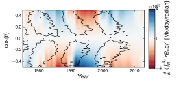
Figure 9: Generation rate of radially integrated toroidal magnetic flux as a function of time and latitude based on KPNO/VTT and SOLIS synoptic magnetograms. Upper left: Flux generation by latitudinal shear. Upper right: Flux generation by radial shear. Lower left: Flux generation by latitudinal and radial shear combined. Lower right: Change of integrated toroidal flux estimated from the sunspot emergence rate. Note the different scaling for the colour bar of this plot. Black contours outline the region where sunspots were observed to emerge.

References

- Antia & Basu (2011) Antia, H. M. & Basu, S. 2011, ApJ, 735, L45
- Baldner & Basu (2008) Baldner, C. S. & Basu, S. 2008, ApJ, 686, 1349
- Barekat et al. (2014) Barekat, A., Schou, J., & Gizon, L. 2014, A&A, 570, L12
- Cally et al. (2003) Cally, P. S., Dikpati, M., & Gilman, P. A. 2003, ApJ, 582, 1190
- Cameron & Schüssler (2015) Cameron, R. & Schüssler, M. 2015, Science, 347, 1333
- Charbonneau (2010) Charbonneau, P. 2010, Living Reviews in Solar Physics, 7, 3, http://www.livingreviews.org/lrsp-2010-3
- Charbonneau (2014) Charbonneau, P. 2014, ARA&A, 52, 251
- Clette et al. (2014) Clette, F., Svalgaard, L., Vaquero, J. M., & Cliver, E. W. 2014, Space Sci. Rev., 186, 35
- Dikpati & Gilman (2009) Dikpati, M. & Gilman, P. A. 2009, Space Sci. Rev., 144, 67
- Gilman et al. (2007) Gilman, P. A., Dikpati, M., & Miesch, M. S. 2007, ApJS, 170, 203
- Gilman & Rempel (2005) Gilman, P. A. & Rempel, M. 2005, ApJ, 630, 615
- Gizon (2004) Gizon, L. 2004, Sol. Phys., 224, 217
- Gizon et al. (2001) Gizon, L., Duvall, Jr., T. L., & Larsen, R. M. 2001, in IAU Symposium, Vol. 203, Recent Insights into the Physics of the Sun and Heliosphere: Highlights from SOHO and Other Space Missions, ed. P. Brekke, B. Fleck, & J. B. Gurman, 189
- Gizon & Rempel (2008) Gizon, L. & Rempel, M. 2008, Sol. Phys., 251, 241
- Hathaway (2011) Hathaway, D. H. 2011, Sol. Phys., 273, 221
- Hathaway & Rightmire (2011) Hathaway, D. H. & Rightmire, L. 2011, ApJ, 729, 80
- Ivanov et al. (2011) Ivanov, V. G., Miletskii, E. V., & Nagovitsyn, Y. A. 2011, Astronomy Reports, 55, 911
- Ivanov & Miletsky (2014) Ivanov, V. G. & Miletsky, E. V. 2014, Geomagnetism and Aeronomy, 54, 907
- Jiang et al. (2013) Jiang, J., Cameron, R. H., Schmitt, D., & Işık, E. 2013, A&A, 553, A128
- Karak et al. (2014) Karak, B. B., Jiang, J., Miesch, M. S., Charbonneau, P., & Choudhuri, A. R. 2014, Space Sci. Rev., 186, 561
- Komm et al. (2015) Komm, R., González Hernández, I., Howe, R., & Hill, F. 2015, Sol. Phys.
- Lawson et al. (2015) Lawson, N., Strugarek, A., & Charbonneau, P. 2015, ApJ, 813, 95
- Liang & Chou (2015) Liang, Z.-C. & Chou, D.-Y. 2015, ApJ, 809, 150
- Muñoz-Jaramillo et al. (2011) Muñoz-Jaramillo, A., Nandy, D., & Martens, P. C. H. 2011, ApJ, 727, L23
- Rempel (2003) Rempel, M. 2003, A&A, 397, 1097
- Schou et al. (1998) Schou, J., Antia, H. M., Basu, S., et al. 1998, ApJ, 505, 390
- SILSO World Data Center (1874-2015) SILSO World Data Center. 1874-2015, International Sunspot Number Monthly Bulletin and online catalogue
- Solanki et al. (2008) Solanki, S. K., Wenzler, T., & Schmitt, D. 2008, A&A, 483, 623
- Spruit (2003) Spruit, H. C. 2003, Sol. Phys., 213, 1
- Spruit (2011) —. 2011, Theories of the Solar Cycle: A Critical View, ed. M. P. Miralles & J. Sánchez Almeida (AGA Special Sopron Book Series, Vol. 4., Springer, Berlin), 39
- Waldmeier (1955) Waldmeier, M. 1955, ”Ergebnisse und Probleme der Sonnenforschung.” (Leipzig, Geest & Portig, 1955. 2. erweiterte Aufl.)
- Zhao & Kosovichev (2004) Zhao, J. & Kosovichev, A. G. 2004, ApJ, 603, 776
- Zita (2010) Zita, E. J. 2010, ArXiv e-prints, 1009.5965