Exceptional Points in a non-Hermitian extension of the Jaynes-Cummings Hamiltonian

Abstract

We consider a generalization of the non-Hermitian ${\mathcal{P}T}$ symmetric Jaynes-Cummings Hamiltonian, recently introduced for studying optical phenomena with time-dependent physical parameters, that includes environment-induced decay. In particular, we investigate the interaction of a two-level fermionic system (such as a two-level atom) with a single bosonic field mode in a cavity. The states of the two-level system are allowed to decay because of the interaction with the environment, and this is included phenomenologically in our non-Hermitian Hamiltonian by introducing complex energies for the fermion system. We focus our attention on the occurrence of exceptional points in the spectrum of the Hamiltonian, clarifying its mathematical and physical meaning.

1 Introduction

Quantum systems whose time evolution can be described by effective non-Hermitian Hamiltonians have been considered since a long time, for example in the framework of irreversible statistical mechanics or for describing decaying unstable systems [1]. Originally introduced to describe phenomenologically these important physical systems, non-Hermitian Hamiltonians have been initially used overlooking the well-known contradictions related to their compatibility with the basic principles of quantum mechanics [2].

In recent years, it has been considered in the literature the possibility to describe realistic physical systems using non-Hermitian Hamiltonians whose eigenvalues are real [3, 4, 5, 6]. This is mathematically meaningful because requiring Hermiticity is a sufficient but not necessary condition to have a real spectrum and a unitary time evolution. In fact, recently, it has been shown that non-Hermitian Hamiltonians with ${\mathcal{P}T}$ (Parity-Time) symmetry can have a real eigenvalue spectrum [4, 7, 8]. The same happens for non-Hermitian but pseudo-symmetric Hamiltonians [9], where the ${\mathcal{P}T}$ symmetry is replaced by a more abstract condition. This new approach has produced several important results in the theory of quantum open systems, quantum optics, balanced gain-loss systems, for example, both from theoretical and experimental point of view (see for example [10] and references therein).

A key point of this topic is to understand what happens when a ${\mathcal{P}T}$ symmetry breaking occurs in a Hamiltonian describing a physical system. As recently investigated (see for example [11]), this may for example happen when one or more physical parameters in the Hamiltonian assume specific values in the complex plane. In more general terms, this aspect is linked to a wider problem addressed in non-Hermitian operator theory, that is the theory of exceptional points (EPs), term introduced in the literature by Kato [12]. Many physical problems are described by Hamiltonians $H(\lambda)$ which manifest dependence on a parameter $\lambda$ linked to quantities accessible in the experimental setting. Generally, the spectrum $E_{n}(\lambda)$ and eigenfunctions $|\psi_{n}(\lambda)\rangle$ of $H(\lambda)$ are analytic functions of $\lambda$. It can occur that, for specific complex values of $\lambda$, two or more energy levels are equal and the corresponding eigenstates coalesce into a single state. It should be emphasized that, in the case of non-Hermitian Hamiltonians, this condition is very different from that of degeneracy common in quantum mechanics. In the presence of EPs, in fact, the coalescence of eigenstates causes the collapse of the subspace dimension to one. Because of this circumstance, the eigenstates no longer form a complete basis and this has very intriguing consequences. For example, ${\mathcal{P}T}$ symmetry is broken [13]. Moreover, EPs may play a very important role in several physical systems, for example in a photonic crystal slab where their presence has been shown to be connected with peaks of reflectivity [10].

In this paper, we shall consider a non-Hermitian generalization of the well-known Jaynes-Cummings (JC) Hamiltonian and investigate the occurrence of EPs in its spectrum. The Jaynes-Cummings model describes a two-level atom interacting with a mode of the quantized electromagnetic field in a cavity [14]; it has been extensively investigated in the literature, in particular in quantum optics. Very recently, we have generalized this model to the non-Hermitian but PT-symmetric case, in order to simulate a time-dependent modulation of the frequency of the two-level-atom or of the cavity mode in the presence of gain-loss [15]. We have also expressed the effective non-Hermitian Jaynes-Cummings Hamiltonian, having an imaginary coupling constant, frequency in term of pseudo-bosons and pseudo-fermions [16, 17], discussing also relevant mathematical and physical aspects of this extension of the Hamiltonian [15].

In this paper we focus our analysis on the occurrence of EPs in the spectrum of this extended Jaynes-Cummings Hamiltonian when the decay of the atomic states is allowed due to interaction with the environment, highlighting the main effects they have on the behavior of the system. In order to make more general our analysis, we have modified the part of the Hamiltonian relative to the two-level system taking as a basis the analysis done in [19], where the authors study nonadiabatic couplings in decaying systems, showing that EPs can influence time-asymmetric quantum-state-exchange mechanism.

The role played by the Jaynes-Cummings model has been crucial to the development of quantum optics and cavity electrodynamics, from both theoretical and experimental points of view [18]. Thus, our extension of the model can shed further light on the dynamics of open optical systems, usually described in terms of non-Hermitian Hamiltonian. Our analysis to elucidate the structure of the exceptional points of the spectrum of the deformed Jaynes-Cummings non-Hermitian Hamiltonian, can be relevant to understand the role of these points in the dynamics of physical systems, such as optical systems, that can be realized in the laboratory. Also, our analysis widens the scenario of applications of the pseudo-bosons and pseudo-fermions formalism.

This paper is organized as follows. In Sec. 2 we introduce our generalized Jaynes-Cummings model allowing the decay of the atomic states; in Sec. 3 we calculate exactly the spectrum and the eigenstates of $H$; in Sec. 4, we discuss the formation of exceptional points in the extended Jaynes-Cummings model; Sec. 5 is dedicated to the discussions of our results and to our conclusive remarks.

2 The non-Hermitian Jaynes-Cummings Hamiltonian

The non-Hermitian extension of the Jaynes-Cummings Hamiltonian we are considering, written in terms of pseudo-bosons and pseudo-fermions, is

$$H=H_{GMM}+\hbar\omega Dd+\epsilon dC+\epsilon^{*}Dc.$$ (1)

where $\omega$ is the frequency of the boson field (a single cavity mode, for example), $\epsilon$ is the boson-fermion coupling constant; $c,C$ and $d,D$ are respectively the pseudo-bosons and pseudo-fermions satisfying the following commutation and anticommutation rules [16, 17]

$$[d\otimes 1\!\!1_{f},D\otimes 1\!\!1_{f}]=1\!\!1_{b}\otimes 1\!\!1_{f}=1\!\!1\,,$$

$$\qquad\{1\!\!1_{b}\otimes c,1\!\!1_{b}\otimes C\}=1\!\!1\,,$$ (2)

while all the other commutators are zero. Our operators act on the Hilbert space $\mathcal{H}:=\mathcal{H}_{b}\otimes\mathcal{H}_{f}$, where $\mathcal{H}_{f}={\mathbb{C}}^{2}$ (fermionic sector) and $\mathcal{H}_{b}$ is infinite dimensional (bosonic sector); $\epsilon$ indicates the coupling constant. The term $H_{GMM}$ in (1) (GMM stands for Gilary, Mailybaev and Moiseyev), originally introduced in [19] and studied later in [20], has the following form:

$$H_{GMM}=\left(\begin{array}[]{cc}\epsilon_{1}-i\Gamma_{1}&\nu_{0}\\ \nu_{0}&\epsilon_{2}-i\Gamma_{2}\\ \end{array}\right),$$ (5)

where $\Gamma_{1}$ and $\Gamma_{2}$ are positive quantities, $\epsilon_{1}$ and $\epsilon_{2}$ are real quantities, and $\nu_{0}$ is complex-valued. This term is an extension of the usual atomic term of the Jaynes-Cummings Hamiltonian and includes possibility of decay of the two atomic states to other states, for example due to the coupling with an environment with a continuous energy spectrum [1]. The quantities $\Gamma_{1}$ and $\Gamma_{2}$ can be related to such phenomenological decay rates.

As shown in [20], $H_{GMM}$ admits a (double) pseudo-fermions representation, and it can be written as $H_{GMM}=\hbar\omega_{0}N_{f}+\rho 1\!\!1$ where $N_{f}=Cc$ and

$$c=\left(\begin{array}[]{cc}\alpha_{11}&\alpha_{12}\\ -\alpha_{11}^{2}/\alpha_{12}&-\alpha_{11}\\ \end{array}\right),\quad C=\left(\begin{array}[]{cc}\beta_{11}&\beta_{12}\\ -\beta_{11}^{2}/\beta_{12}&-\beta_{11}\\ \end{array}\right),$$ (6)

$$\left\{\begin{array}[]{ll}\hbar\omega^{\pm}_{0}\gamma_{\pm}=\nu_{0},\\ \alpha_{\pm}=\frac{1}{2\nu_{0}}\left(-\Delta\epsilon+i\Delta\Gamma\mp\sqrt{(-\Delta\epsilon+i\Delta\Gamma)^{2}+4\nu_{0}^{2}}\right),\\ \beta_{\pm}=\frac{1}{2\nu_{0}}\left(-\Delta\epsilon+i\Delta\Gamma\pm\sqrt{(-\Delta\epsilon+i\Delta\Gamma)^{2}+4\nu_{0}^{2}}\right),\\ \rho_{\pm}=\frac{1}{2}\left(\tilde{\epsilon}-i\Gamma\pm\sqrt{(-\Delta\epsilon+i\Delta\Gamma)^{2}+4\nu_{0}^{2}}\right),\end{array}\right.$$ (11)

being $\alpha=\frac{\alpha_{11}}{\alpha_{12}}$, $\beta=\frac{\beta_{11}}{\beta_{12}}$, $\gamma_{\pm}=\alpha_{12}\beta_{11}-\alpha_{11}\beta_{12}=\alpha_{12}\beta_{12}(\beta_{\pm}-\alpha_{\pm})$, $\Delta\epsilon=\epsilon_{2}-\epsilon_{1}$, $\Delta\Gamma=\Gamma_{2}-\Gamma_{1}$, $\tilde{\epsilon}=\epsilon_{2}+\epsilon_{1}$ and $\Gamma=\Gamma_{2}+\Gamma_{1}$. We see that we have two possible solutions (the plus solution and the minus solution) and that both solutions admit two free parameters. For instance, choosing $\alpha_{+}$ above, implies that $\alpha_{11}$ is fixed if we first fix $\alpha_{12}$. Hence, for each given choice of $\alpha_{12}$ we have a different solution for $c$. It should be noted that the following condition for the pseudo-fermions existence (see [20]),

$$-\gamma_{\pm}^{2}=\alpha_{12}\beta_{12},$$ (12)

must be satisfied, otherwise $H_{GMM}$ can be expressed as standard fermionic operator ($C=c^{{\dagger}}$) or it cannot be diagonalized. Since $\gamma_{\pm}=\alpha_{12}\beta_{12}(\beta_{\pm}-\alpha_{\pm})$ and $\gamma_{\pm}^{2}=-\alpha_{12}\beta_{12}$, we find that, whichever $\alpha_{\pm}\neq\beta_{\pm}$, by taking

$$\alpha_{12}\beta_{12}=\frac{-\nu_{0}^{2}}{(-\Delta\epsilon+i\Delta\Gamma)^{2}+4\nu_{0}^{2}},$$

the condition (12) is satisfied. On the other hand, this is not possible if $\alpha_{\pm}=\beta_{\pm}$, that is $(-\Delta\epsilon+i\Delta\Gamma)^{2}=-4\nu_{0}^{2}$; in this case the eigenvalues of $H_{GMM}$ coalesce to the value $\frac{1}{2}(\tilde{\epsilon}-i\Gamma)$. Notice that all the above conditions lead to the link of $\omega_{0}$ with the parameters defining $H_{GMM}$, as the following condition must be satisfied to ensure that (12) is valid:

$$\hbar\omega_{0}^{\pm}=\pm\sqrt{4\nu_{0}^{2}+(-\Delta\epsilon+i\Delta\Gamma)^{2}}.$$ (13)

Notice that this in general means that $\omega_{0}^{\pm}$ are complex quantities. To simplify the treatment we restrict here to the principal square root. This relation will prove to be very important in the following because it highlights that the formation of EPs depends on the phenomenological parameters $\Gamma_{1}$ and $\Gamma_{2}$, justifying their introduction in Hamiltonian (1).

3 Eigenstates and eigenvalues of $H$

With a simple extension of the procedure discussed in [15] (see also [18]) we can rewrite $H$ in a diagonal form. For that, we first introduce a global non self-adjoint number operator, analogous to the total-excitations-number operator,

$$N=Dd+Cc,$$

and the map defined as

$$T=\textrm{exp}\{-\theta(4|\epsilon|^{2}N)^{-1/2}(\epsilon dC+\epsilon^{\ast}Dc)\},$$ (14)

where $\theta$ is the operator defined by $\sin\theta=-(4|\epsilon|^{2}N)^{1/2}\Delta^{-1}$ and $\cos\theta=-\delta\Delta^{-1}$, where $\delta=\hbar(\omega_{0}-\omega)$ is the detuning between the energies of the two fields and $\Delta=\left(\delta^{2}+4|\epsilon|^{2}N\right)^{1/2}$. By defining the dressed operators $\hat{C}=TCT^{-1},\hat{c}=TcT^{-1},\hat{D}=TDT^{-1},\hat{d}=TdT^{-1}$ it is easy to check that they are tensor products of pseudo-bosonic and pseudo-fermionic operators satisfying themselves commutation rules analogous to (2), and the Hamiltonian $H$ can be written in a diagonal form as:

$$H=\left(\hbar\omega-\hat{\Delta}\right)(\hat{C}\hat{c}-\frac{1}{2})+\hbar\omega\hat{D}\hat{d}+\left(\frac{\hbar\omega_{0}}{2}+\rho\right)1\!\!1.$$ (15)

Following the general procedures used for the pseudo-fermions and pseudo-bosons operators in [16], we can construct the eigenvectors of $H$ and $H^{\dagger}$ in the framework of deformed canonical commutation relations and canonical anti-commutation relations. We know that two non-zero vectors $\hat{\varphi}_{0}$ and $\hat{\psi}_{0}$ do exist in $\mathcal{H}_{b}$ such that, if $\hat{\eta}_{0}$ and $\hat{\mu}_{0}$ are two vectors of the fermionic Hilbert space $\mathcal{H}_{f}$ annihilated respectively by $\hat{c}$ and $\hat{C}^{\dagger}$, we have

$$\left(\hat{d}\otimes\hat{1}\!\!1_{f}\right)\hat{\Phi}_{0,0}=\left(\hat{1}\!\!1_{b}\otimes\hat{c}\right)\hat{\Phi}_{0,0}=0,$$ (16)

as well as

$$\left(\hat{D}^{\dagger}\otimes\hat{1}\!\!1_{f}\right)\hat{\Psi}_{0,0}=\left(\hat{1}\!\!1_{b}\otimes\hat{C}^{\dagger}\right)\hat{\Psi}_{0,0}=0\,,$$ (17)

where $\hat{\Phi}_{0,0}:=\hat{\varphi}_{0}\otimes\hat{\eta}_{0}$ and $\hat{\Psi}_{0,0}:=\hat{\psi}_{0}\otimes\hat{\mu}_{0}$. As already pointed out in [17, 23], it is convenient to assume that $\hat{\varphi}_{0}$ and $\hat{\psi}_{0}$ belong to a dense domain ${\mathcal{D}}$ of $\mathcal{H}_{b}$, which is left stable under the action of $d$, $D$, and their adjoint. As for $\hat{\eta}_{0}$ and $\hat{\mu}_{0}$, these vectors surely exist in $\mathcal{H}_{f}$ and belong to the domain of all the (pseudo-fermionic) operators involved into the game, as one can easily deduce from the fact that $\mathcal{H}_{f}$ is a finite dimensional vector space. If such a ${\mathcal{D}}$ exists, then we can use the two vacua $\hat{\Phi}_{0,0}$ and $\hat{\Psi}_{0,0}$ to construct two different sets of vectors, ${\cal F}_{\hat{\Phi}}:=\{\hat{\Phi}_{n,k},\,n\geq 0,\,k=0,1\}$ and ${\cal F}_{\hat{\Psi}}:=\{\hat{\Psi}_{n,k},\,n\geq 0,\,k=0,1\}$, all belonging to ${\mathcal{D}}\otimes\mathcal{H}_{f}$, as follows:

$$\hat{\Phi}_{n,k} = \left(\frac{1}{\sqrt{n!}}\hat{D}^{n}\otimes\hat{C}^{k}\right)\hat{\Phi}_{0,0}\,,$$ (18)

$$= \left(\frac{1}{\sqrt{n!}}\hat{D}^{n}\hat{\varphi}_{0}\right)\otimes\left(\hat{C}^{k}\hat{\eta}_{0}\right):=\hat{\varphi}_{n}\otimes\hat{\eta}_{k}\,\$$

and

$$\hat{\Psi}_{n,k} = \left(\frac{1}{\sqrt{n!}}\hat{d^{\dagger}}^{n}\otimes\hat{c^{\dagger}}^{k}\right)\hat{\Psi}_{0,0}$$ (19)

$$= \left(\frac{1}{\sqrt{n!}}\hat{d^{\dagger}}^{n}\hat{\psi}_{0}\right)\otimes\left(\hat{c^{\dagger}}^{k}\hat{\mu}_{0}\right):=\hat{\psi}_{n}\otimes\hat{\mu}_{k}\,,$$

with obvious notations, where $n=0,1,2,\ldots$ and $k=0,1$. It is now easy to check that

$$H\hat{\Phi}_{n,k}=E_{n,k}\hat{\Phi}_{n,k},\qquad H^{\dagger}\hat{\Psi}_{n,k}=E_{n,k}^{*}\hat{\Psi}_{n,k}\,,$$ (20)

where the eigenvalues are

$$E_{n,k}=\hbar\omega n+\frac{\hbar\omega_{0}}{2}+\rho+\left[\hbar\omega-\left(\delta^{2}+4|\epsilon|^{2}(n+k)\right)^{1/2}\right]\left(k-\frac{1}{2}\right).$$ (21)

Also, if the normalization of $\hat{\Phi}_{0,0}$ and $\hat{\Psi}_{0,0}$ is chosen in such a way that $\left<\hat{\Phi}_{0,0},\hat{\Psi}_{0,0}\right>=1$, then

$$\left<\hat{\Phi}_{n,k},\hat{\Psi}_{m,l}\right>=\left<\hat{\varphi}_{n},\hat{\psi}_{m}\right>_{\mathcal{H}_{b}}\left<\hat{\eta}_{k},\hat{\mu}_{l}\right>_{\mathcal{H}_{f}}=\delta_{n,m}\delta_{l,k}\,.$$ (22)

Here $\left<.,.\right>_{\mathcal{H}_{b}}$ and $\left<.,.\right>_{\mathcal{H}_{f}}$ are respectively the scalar products in $\mathcal{H}_{b}$ and in $\mathcal{H}_{f}$.

4 Exceptional Points formation

In this section we investigate the formation of exceptional points in our extended Jaynes-Cummings Hamiltonian. It is convenient to introduce the analogous pseudo-structures given by the conditions (16-19) for the non diagonal form (1) of our Hamiltonian. As before, we can also define the two set of vectors, ${\cal F}_{\Phi}:=\{\Phi_{n,k},\,n\geq 0,\,k=0,1\}$ and ${\cal F}_{\Psi}:=\{\Psi_{n,k},\,n\geq 0,\,k=0,1\}$, all belonging to ${\mathcal{D}}\otimes\mathcal{H}_{f}$, as follows:

$$\Phi_{n,k}=\left(\frac{1}{\sqrt{n!}}D^{n}\otimes C^{k}\right)\Phi_{0,0} = \left(\frac{1}{\sqrt{n!}}D^{n}\varphi_{0}\right)\otimes\left(C^{k}\eta_{0}\right)=:\varphi_{n}\otimes\eta_{k},$$

$$\Psi_{n,k}=\left(\frac{1}{\sqrt{n!}}{d^{\dagger}}^{n}\otimes{c^{\dagger}}^{k}\right)\Psi_{0,0} = \left(\frac{1}{\sqrt{n!}}{d^{\dagger}}^{n}\psi_{0}\right)\otimes\left({c^{\dagger}}^{k}\mu_{0}\right)=:\psi_{n}\otimes\mu_{k}\,,$$

and, as usual,

$$\left(d\otimes\hat{1}\!\!1_{f}\right)\Phi_{0,0}=\left(1\!\!1_{b}\otimes c\right)\Phi_{0,0}=0,$$ (23)

$$\left(D^{\dagger}\otimes 1\!\!1_{f}\right)\Psi_{0,0}=\left(1\!\!1_{b}\otimes C^{\dagger}\right)\Psi_{0,0}=0,$$ (24)

and

$$\left<\Phi_{n,k},\Psi_{m,l}\right>=\delta_{n,m}\delta_{l,k}.$$ (25)

It is easy to check that, in terms of the vectors given above, the eigenvalues of $H$ and $H^{\dagger}$ can be rewritten in order to satisfy the following conditions:

$$H\left(\Phi_{n-1,1}+\lambda^{\pm}_{n}\Phi_{n,0}\right) = E^{\pm}_{n}\left(\Phi_{n-1,1}+\lambda^{\pm}_{n}\Phi_{n,0}\right),$$ (26)

$$H^{\dagger}\left(\Psi_{n-1,1}+\xi^{\pm}_{n}\Psi_{n,0}\right) = E^{\pm*}_{n}\left(\Psi_{n-1,1}+\xi^{\pm}_{n}\Psi_{n,0}\right),$$ (27)

where

$$E^{\pm}_{n}=\hbar\omega(n-\frac{1}{2})+\frac{\hbar\omega_{0}}{2}+\rho\pm\frac{\left(\delta^{2}+4|\epsilon|^{2}n\right)^{1/2}}{2},$$

and

$$\lambda^{\pm}_{n}=\frac{-\delta\pm(\delta^{2}+4|\epsilon|^{2}n)^{1/2}}{2\epsilon\sqrt{n}},\xi^{\pm}_{n}=\frac{-\delta^{*}\pm\left((\delta^{*})^{2}+4|\epsilon|^{2}n\right)^{1/2}}{2\epsilon\sqrt{n}}.$$

For each $n$, we have $E^{+}_{n}=E_{n,0}$ and $E^{-}_{n}=E_{n-1,1}$. It thus follows from (20) and (27) that

$$\hat{\Phi}_{n,0} = g^{n,0}_{\hat{\Phi}}\left(\Phi_{n-1,1}+\lambda^{+}_{n}\Phi_{n,0}\right),\hat{\Psi}_{n,0}=g^{n,0}_{\hat{\Psi}}\left(\Psi_{n-1,1}+\xi^{+}_{n}\Psi_{n,0}\right),$$

$$\hat{\Phi}_{n-1,1} = g^{n-1,1}_{\hat{\Phi}}\left(\Phi_{n-1,1}+\lambda^{-}_{n}\Phi_{n,0}\right),\hat{\Psi}_{n-1,1}=g^{n-1,1}_{\hat{\Psi}}\left(\Psi_{n-1,1}+\xi^{-}_{n}\Psi_{n,0}\right),$$

being $g_{\Phi},g_{\Psi}$ appropriate normalization constants given by the bi-orthogonality conditions (22).

If we now consider the case in which $\delta^{2}+4|\epsilon|^{2}n=0$, then $E_{n}^{+}=E_{n}^{-},\lambda_{n}^{+}=\lambda_{n}^{-}$. Therefore, the couples of vectors $\hat{\Phi}_{n,0},\hat{\Phi}_{n-1,1}$ and $\hat{\Psi}_{n,0},\hat{\Psi}_{n-1,1}$ being proportional, are linearly dependent. This condition implies that $\delta$ is purely imaginary, so that $\hbar(\omega_{0}-\omega)=i\tau$ with $\tau=\tau^{\pm}=\pm 2|\epsilon|\sqrt{n}$. Varying $\tau$ leads to the situation shown in Fig.0(c) for $n=100$. For $\tau<\tau^{-}$ and $\tau>\tau^{+}$, the eigenvalues $E_{n}^{+},E_{n}^{-}$ relative to $n$-excitation space have same real parts and different imaginary parts. For $\tau^{-}\leq\tau\leq\tau^{+}$, the eigenvalues have different real parts and the same imaginary parts. At $\tau=\tau^{\pm}$ the eigenvalues coalesce to the value $\hbar\omega(n-\frac{1}{2})+\frac{\hbar\omega_{0}}{2}+\rho$; also, due to the presence of two branch points in $\tau^{\pm}$ for $E_{n}^{\pm}(\tau)$, we obtain that encircling the points $\tau^{\pm}$ in the complex plane interchanges the two eigenvalues. In fact considering an arbitrary closed loop $s^{\pm}(\theta)=\tau^{\pm}+re^{i\theta}$ around $\tau^{\pm}$ leads to $E_{n}^{\pm}(s(0))=E_{n}^{\mp}(s(2\pi))$.

It is worth noting that at $\tau=\tau^{\pm}$ the condition $\lambda_{n}^{+}=\lambda_{n}^{-}=-\frac{\delta}{2|\epsilon|\sqrt{n}}$ leads to the vanishing of the scalar products $\left<\hat{\Phi}_{n,0},\hat{\Psi}_{n,0}\right>$ and $\left<\hat{\Phi}_{n-1,1},\hat{\Psi}_{n-1,1}\right>$. In fact

$$\left<\hat{\Phi}_{n,0},\hat{\Psi}_{n,0}\right>=g^{n,0*}_{\hat{\Phi}}g^{n,0}_{\hat{\Psi}}\left(\left<\Phi_{n-1,1},\Psi_{n-1,1}\right>-\frac{\tau^{2}}{4|\epsilon|^{2}n}\left<\Phi_{n,0},\Psi_{n,0}\right>\right)=0,$$ (28)

because $\tau^{\pm}=\pm 2|\epsilon|\sqrt{n}$. Analogously $\left<\hat{\Phi}_{n-1,1},\hat{\Psi}_{n-1,1}\right>$=0. These conditions are typical of the EPs formation at $\tau^{\pm}$, [21]. Fig.0(f) shows that only for $n=100$, for our particular choice of parameters, $E_{n}^{+}=E_{n}^{-}$, so that the related eigenstates coalesce. More important, our results show that at the EPs the pseudo-structure in terms of pseudo-fermions and pseudo-bosons operator is no more valid. In fact it has been shown that, in presence of an EP, the coefficients defining the operators $c$ and $C$, see (6), cannot satisfy the necessary condition (12) (see [20]).

Notice that through (13), we obtain that the EPs formation is compatible only with the following choices of $\omega$

$$\hbar\omega^{\pm}=\pm\sqrt{4\nu_{0}^{2}+(-\Delta\epsilon+i\Delta\Gamma)^{2}}-i\tau,$$ (29)

where it is evident that EPs form only for an appropriate choice of $\nu_{0}$ and of the relative differences $\Delta\epsilon,\Delta\Gamma$ of the parameters $\epsilon_{1,2}$ and $\Gamma_{1,2}$ in (1), which is related to $\omega$ and $\omega_{0}$. It must be emphasized that by manipulating parameters present in the Hamiltonian (1), it is possible to change the position of the EPs in the complex plane. In Figs.0(i)-1 we show the eigenvalues $E_{n}^{\pm}$ in the complex plane by varying respectively $\Delta\epsilon,\Delta\Gamma$ and $\nu_{0}$. This opens up the prospects of a kind of engineering of EPs in order to exploit their impact on the dynamics of the physical system in which they appear. For example, this can be obtained by appropriately changing the decay rates $\Gamma_{1}$ and $\Gamma_{2}$ (see [22] and references therein).

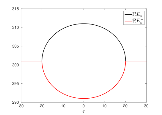
(a)

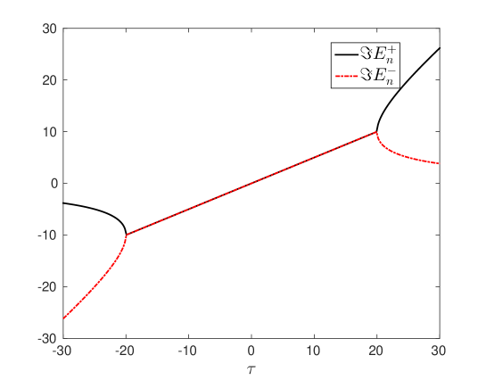
(b)

(c) . Real (a) and imaginary (b) parts of the eigenvalues $E_{n}^{\pm}$ for $n=100$ as function of the parameter $\tau=-i(\hbar\omega_{0}-\hbar\omega)$. Other parameters are $\epsilon=1,\rho=1,\omega=3$; units are such that $\hbar=1$. At the EPs $\tau=\pm 20$ eigenvalues coalesce so that $E_{n}^{+}=E_{n}^{-}$.

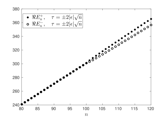
(d)

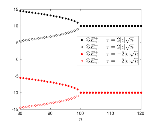
(e)

(f) . Real (a) and imaginary (b) parts of the eigenvalues $E_{n}^{\pm}$ as function of the parameter $n$ for $\tau=i(\hbar\omega_{0}-\hbar\omega)$ (black lines) and $\tau=-i(\hbar\omega_{0}-\hbar\omega)$ (red lines). Other parameters are $\epsilon=1,\rho=1,\omega=3$; units are such that $\hbar=1$. At $n=100$ the EPs are formed, and eigenvalues coalesce so that $E_{n}^{+}=E_{n}^{-}$.

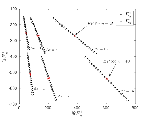
(g)

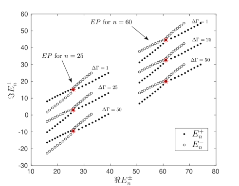
(h)

(i) Eigenvalues $E_{n}^{\pm}$ in the complex plane for various values of $n$. In a) eigenvalues are obtained by taking $\nu_{0}=1,\epsilon_{1}=0.5,\Gamma_{1}=0,\Gamma_{2}=1$, $\omega_{0}=\sqrt{4+(\Delta\epsilon+i)^{2}}$, $\rho=0.5(1+\Delta\epsilon-i+\sqrt{4+(\Delta\epsilon+i)^{2}})$ and $\omega=\sqrt{4+(\Delta\epsilon+i)^{2}}-2i\sqrt{\tilde{n}}$, for $\tilde{n}=25$ and $\tilde{n}=40$, $\epsilon_{2}$ is varied according to the chosen value of $\Delta\epsilon$. In b) eigenvalues are obtained by taking $\epsilon_{1}=\epsilon_{2}=0.5,\Gamma_{1}=0,\omega=1+i$, $\nu_{0}=0.5\sqrt{(1+i-2i\sqrt{\tilde{n}})^{2}-(i\Delta\Gamma^{2})},\omega_{0}=1+3i\sqrt{\tilde{n}},\rho=0.5(2-i\Delta\Gamma+3i\sqrt{n})$, for $\tilde{n}=25$ and $\tilde{n}=60$, $\Gamma_{2}$ is varied according to the chosen value of $\Delta\Gamma$. At the EPs, the eigenvalues coalesce, marked in the plots by the red $*$

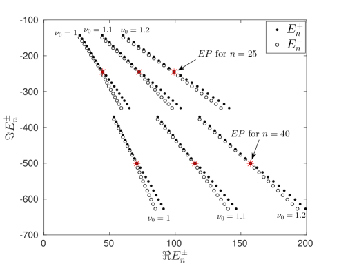
Figure 1: Eigenvalues $E_{n}^{\pm}$ in the complex plane for various values of $\nu_{0}$ and $n$. Parameters are $\epsilon_{1}=\epsilon_{2}=0.5,\Gamma_{1}=0,\Gamma_{2}=1$,$\omega=1+1i,\omega_{0}=$, $\rho=0.5(1-i1+\omega_{0})$, $\omega=\sqrt{4+(\Delta\epsilon+i1)^{2}}-2i\sqrt{\tilde{n}}$, for $\tilde{n}=25$ and $\tilde{n}=40$. At the EPs the eigenvalues coalesce, marked in the plot by the red $*$

5 Conclusions and perspectives

In this paper we have considered the formation of exceptional points in a non-Hermitian Jaynes-Cummings Hamiltonian, that generalizes the Hamiltonian of a two-level atom interacting with a single cavity field mode to the case in which dissipation and decay are phenomenologically included.

The results obtained in this paper show the exceptional points identified in the non-Hermitian Jaynes-Cummings Hamiltonian (1), have the same structure obtained in [24, 25].

From a mathematical point of view, this is due to the fact that, for a two-level system, the eigenvalues contain in their mathematical expression a square root as that of a second-degree algebraic equation. The collapse of the eigenvalues and the formation of EPs depend on the vanishing of the square-root argument for specific values of the physical parameters involved. On the other hand, the interchange properties of the eigenvalues when EPs are encircled can be interpreted as an effect due to the branch points of the square root when analyzed as a function in the complex plane. Also, encircling EPs causes the switch of the eigenfunctions, showing that their relative phases are not rigid. From a physical point of view, this behavior can be interpreted as a manifestation of the capability of the system to align itself with the environment to which it is coupled (see also [25]).

The main novelties introduced in this paper concern with the analysis of the exceptional points for the spectrum of a non-Hermitian Jaynes-Cummings Hamiltonian expressed in terms of a mixture of pseudo-fermions and pseudo-bosons (previous analysis were focused on EPs in non-Hermitian pseudo-fermionic operators, [20]). Thus, the application range of this theory on pseudo-particles is here extended. We wish to stress that the existence of a pseudo-structure is deeply related to the existence of EPs: in fact, as we have shown in Section 4, the spontaneous generation of the EPs implies that the biorthogonality condition (22), which characterizes the pseudo-structure we have introduced, is no more satisfied. This is expected, since a pseudofermionic or pseudobosonic structure is intrinsically connected with the existence of non coincident eigenvalues. Moreover, the deformed Jaynes-Cummings model analyzed in [15] and in this paper, could be used to further investigate the role played by EPs on interaction between atomic systems and the electromagnetic field, including damping or amplifying processes, which is of fundamental importance in quantum optics.

References

- [1] W.C. Schieve and L.P. Horwitz, Quantum Statistical Mechanics, Cambridge Unibversity Press, Cambridge 2009.
- [2] G. Barton, Introduction to Advanced Field Theory, John Wiley & Sons, 1963.
- [3] A. Mostafazadeh, Pseudo-Hermitian Representation of Quantum Mechanics, Int. J. Geom. Meth. Mod. Phys. 7, 1191 (2010).
- [4] C. M. Bender and S. Boettcher, Real Spectra of Non-Hermitian Hamiltonian Having Symmetry, Phys. Rev. Lett. 80, 5243 (1998).
- [5] A. Mostafazadeh, Non-Hermitian Hamiltonians with a real spectrum and their physical applications, Pramana-J. Phys. 73, 269 (2009).
- [6] C. M. Bender, M. V. Berry, and A. Mandilara, Generalized Symmetry and Real Spectra, J. of Phys. A: Math. and Gen. 35, L467 (2002).
- [7] C. M. Bender, D. C. Brody, and H. F. Jones Complex Extension of Quantum Mechanics, Phys. Rev. Lett. 89, 270401 (2002).
- [8] C. M. Bender, Making sense of non-Hermitian Hamiltonians, Rep. Prog. Phys. 70, 947 (2007).
- [9] A. Mostafazadeh, Pseudo-Hermiticity versus -Symmetry: the necessary condition for the reality of the spectrum of a non-Hermitian Hamiltonian, J. Math. Phys., 43, 205 (2002).
- [10] B. Zhen, C. W. Hsu, Y. Igarashi, L. Lu, I. Kaminer, A. Pick, S.-L. Chua, J. D. Joannopoulos, and M. Soljac̆ić, Spawning rings of exceptional points out of Dirac cones, Nature 525, 354 (2015).
- [11] W.D. Heiss, Exceptional points of non-Hermitian operators, J. Phys. A 37, 6 (2004).
- [12] T. Kato, Perturbation theory of linear operators, Springer, Berlin, 1966.
- [13] I. Rotter and J. P. Bird, A review of recent progress in the physics of open quantum systems: theory and experiment , arXiv:1507.08478, accepted for Report on Progress in Physics.
- [14] E.T. Jaynes, F.W. Cummings, Comparison of quantum and semiclassical radiation theories with application to the beam maser, Proc. IEEE 51, 89 (1963).
- [15] F. Bagarello, M. Lattuca, R. Passante, L. Rizzuto, and S. Spagnolo, Non-Hermitian Hamiltonian for a modulated Jaynes-Cummings model with symmetry, Phys. Rev. A 91, 042134 (2015).
- [16] F. Bagarello, Deformed canonical (anti-)commutation relations and non hermitian Hamiltonians, in Non-selfadjoint operators in quantum physics: Mathematical aspects, F. Bagarello, J. P. Gazeau, F. Szafraniec and M. Znojil, Eds, J. Wiley and Sons, 2015.
- [17] F. Bagarello and M. Lattuca, pseudo bosons in quantum models, Phys. Lett. A 377, 3199 (2013).
- [18] G. Compagno, R. Passante, and F. Persico, Atom-Field Interactions and Dressed Atoms, Cambridge University Press, Cambridge 1995.
- [19] I. Gilary, A. A. Mailybaev, and N. Moiseyev, Time-asymmetric quantum-state-exchange mechanism, Phys. Rev. A, 88, 010102(R) (2013).
- [20] F. Bagarello, F. Gargano, Model pseudofermionic systems: connections with exceptional points, Phys. Rev. A, 89, 032113 (2014).
- [21] W.D. Heiss, The physics of exceptional points, J. Phys. A: Math. Theor. 45, 444016 (2012).
- [22] I. E. Linington, B. M. Garraway, Control of atomic decay rates via manipulation of reservoir mode frequencies, J. Phys. B: At. Mol. Opt. Phys. 39, 3383 (2006).
- [23] F. Bagarello, F. Gargano, D. Volpe, -Deformed Harmonic Oscillators, Int. J. of Theor. Phys., 54(11), 4110 (2015).
- [24] M. Müller, I. Rotter, Exceptional points in open quantum systems, J. of Phys. A: Math. and Gen., 41, 244018 (2008).
- [25] H. Eleuch, I. Rotter, Exceptional points in open and symmetric systems, Acta Polytech. 54, 106 (2014).